Dynamical properties of endomorphisms, multiresolutions, similarity-and orthogonality relations

Abstract.

We study positive transfer operators $R$ in the setting of general measure spaces $\left(X,\mathscr{B}\right)$. For each $R$, we compute associated path-space probability spaces $\left(\Omega,\mathbb{P}\right)$. When the transfer operator $R$ is compatible with an endomorphism in $\left(X,\mathscr{B}\right)$, we get associated multiresolutions for the Hilbert spaces $L^{2}\left(\Omega,\mathbb{P}\right)$ where the path-space $\Omega$ may then be taken to be a solenoid. Our multiresolutions include both orthogonality relations and self-similarity algorithms for standard wavelets and for generalized wavelet-resolutions. Applications are given to topological dynamics, ergodic theory, and spectral theory, in general; to iterated function systems (IFSs), and to Markov chains in particular.

1. Introduction

The purpose of our paper is two-fold, first (1) to make precise a setting of general measure spaces, and families of positive transfer operators $R$, and for each $R$ to compute the associated path-space measures $\left(\Omega,\mathbb{P}\right)$; and secondly (2) to create multiresolutions (Sections 5.1 and 5.3) in the corresponding Hilbert spaces $L^{2}\left(\Omega,\mathbb{P}\right)$ of square integrable random variables.

We shall use the notion of “transfer operator” in a wide sense so that our framework will encompass diverse settings from mathematics and its applications, including statistical mechanics where the relevant operators are often referred to as Ruelle-operators (Definitions 2.1 and 5.5; and we shall use the notation $R$ for transfer operator for that reason.) See, e.g,. [Sto13, Rug16, MU15, JR05, Rue04]. But we shall also consider families of transfer operators arising in harmonic analysis, including spectral analysis of wavelets (5.2), in ergodic theory of endomorphisms in measure spaces (2.2 and 10), in Markov random walk models, in the study of transition processes in general; and more.

In the setting of endomorphisms and solenoids, we obtain new multiresolution orthogonality relations in the Hilbert space of square integrable random variables. We shall further draw parallels between our present infinite-dimensional theory and the classical finite-dimensional Perron-Frobenius theorems (see, e.g., [JR05, Rue04, GH16, MU15, Pap15, FT15]); the latter referring to the case of finite positive matrices.

To make this parallel, it is helpful to restrict the comparison of the infinite-dimensional theory to the case of the Perron-Frobenius (P-F) for finite matrices in the special case when the spectral radius is 1.

Our present study of infinite-dimensional versions of P-F transfer operators includes theorems which may be viewed as analogues of many points from the classical finite-dimensional P-F case; for example, the classical respective left and right Perron-Frobenius eigenvectors now take the form in infinite-dimensions of positive $R$ invariant measures (left), and the infinite-dimensional right P-F vector becomes a positive harmonic function. Of course in infinite-dimensions, we have more non-uniqueness than is implied by the classical matrix theorems, but we also have many parallels. We even have infinite-dimensional analogues of the P-F limit theorems from the classical matrix case.

Important points in our present consideration of transfer operators are as follows: We formulate a general framework, a list of precise axioms, which includes a diverse host of applications. In this, we separate consideration of the transfer operators as they act on functions on Borel spaces $\left(X,\mathscr{B}\right)$ on the one hand, and their Hilbert space properties on the other hand. When a transfer operator is given, there is a variety of measures compatible with it, and we shall discuss both the individual cases, as well as the way a given transfer operator is acting on a certain universal Hilbert space (Definitions 9.1 and 9.2). The latter encompasses all possible probability measures on the given Borel space $\left(X,\mathscr{B}\right)$. This yields new insight, and it helps us organize our results on ergodic theoretic properties connected to the theory of transfer operators, 10.

2. Measure spaces

In the next two sections we make precise the setting of general measure spaces, and families of positive transfer operators $R$, and we study a number of convex sets of measures computed directly from $R$.

The general setting is as follows:

Definition 2.1.

1. $\left(X,\mathscr{B}\right)$ is a fixed measure space, i.e., $\mathscr{B}$ is a fixed sigma-algebra of subsets of a set $X$. Usually, we assume, in addition, that $\left(X,\mathscr{B}\right)$ is a Borel space.

2. Notation: $\sigma:X\rightarrow X$ is a measurable endomorphism, i.e., $\sigma^{-1}\left(\mathscr{B}\right)\subset\mathscr{B}$, $\sigma^{-1}\left(A\right)\in\mathscr{B}$ for all $A\in\mathscr{B}$; and we assume further that $\sigma\left(X\right)=X$, i.e., $\sigma$ is onto.

3. $\mathscr{F}\left(X,\mathscr{B}\right)$ = the algebra of all measurable functions on $\left(X,\mathscr{B}\right)$.

4. By a transfer operator $R$, we mean that $R:\mathscr{F}\left(X,\mathscr{B}\right)\longrightarrow\mathscr{F}\left(X,\mathscr{B}\right)$ is a linear operator s.t. (2.1) $\&$ (2.2) hold, where:

   $$f\geq 0\Longrightarrow R\left(f\right)\geq 0;\;\text{and}$$ (2.1)

   $$R\left(\left(f\circ\sigma\right)g\right)=fR\left(g\right),\;\forall f,g\in\mathscr{F}\left(X,\mathscr{B}\right).$$ (2.2)

   (See, e.g., [Sto13, Rug16, MU15, JR05, Rue04].)

5. We assume that

   $$R\mathbbm{1}=\mathbbm{1}$$ (2.3)

   where $\mathbbm{1}$ denotes the constant function “one” on $X$, and we restrict consideration to the case of real valued functions. Subsequently, condition (2.3) will be relaxed.

6. If $\lambda$ is a measure on $\left(X,\mathscr{B}\right)$, we set $\lambda R$ to be the measure specified by

   $$\int_{X}f\,d\left(\lambda R\right):=\int_{X}R\left(f\right)d\lambda,\;\forall f\in\mathscr{F}\left(X,\mathscr{B}\right).$$ (2.4)

7. We shall assume separability, for example we assume that $\left(X,\mathscr{B},\lambda\right)$, as per (1)–(6), has the property that $L^{2}\left(X,\mathscr{B},\lambda\right)$ is a separable Hilbert space.

Remark 2.2.

The role of the endomorphism $X\xrightarrow{\;\sigma\;}X$ is fourfold:

1. $\sigma$ is a point-transformation, generally not invertible, but assumed onto.

2. We also consider $\sigma$ as an endomorphism in the fixed measure space $\left(X,\mathscr{B}\right)$ and so $\sigma^{-1}:\mathscr{B}\rightarrow\mathscr{B}$ where

   $$\sigma^{-1}\left(\mathscr{B}\right) =\left\{\sigma{}^{-1}\left(A\right)\mid A\in\mathscr{B}\right\},\>\text{and}$$

   $$\sigma^{-1}\left(A\right) :=\left\{x\in X\mid\sigma\left(x\right)\in A\right\},$$

   so $\sigma^{-1}\left(\mathscr{B}\right)\subset\mathscr{B}$.

3. We shall assume further that $\sigma$ is ergodic [Yos80, KP16], i.e., that

   $$\bigcap_{n=1}^{\infty}\sigma^{-n}\left(\mathscr{B}\right)=\left\{\emptyset,X\right\}$$

   modulo sets of $\lambda$-measure zero.

4. $\sigma$ defines an endomorphism in the space $\mathscr{F}\left(X,\mathscr{B}\right)$ of all measurable functions via $f\mapsto f\circ\sigma$.

3. Sets of measures for $\left(X,\mathscr{B},\sigma,R\right)$

We shall undertake our analysis of particular transfer operators/endomorphisms in a fixed measure space $\left(X,\mathscr{B}\right)$ with the use of certain sets of measures on $\left(X,\mathscr{B}\right)$. These sets play a role in our theorems, and they are introduced below. We present examples of transfer operators associated to iterated function systems (IFSs) in a stochastic framework. 3.3 and 3.8 prepare the ground for this, and the theme is resumed systematically in 4.2 below.

For positive measures $\lambda$ and $\mu$ on $\left(X,\mathscr{B}\right)$, we shall work with absolute continuity, written $\lambda\ll\mu$.

Definition 3.1.

$\lambda\ll\mu$ iff (Def.) [$A\in\mathscr{B}$, $\mu\left(A\right)=0$ $\Longrightarrow$ $\lambda\left(A\right)=0$]. Moreover, when $\lambda\ll\mu$, we denote the Radon-Nikodym derivative $\frac{d\lambda}{d\mu}$. In detail,

$$\int_{B}\left(\frac{d\lambda}{d\mu}\right)d\mu=\lambda\left(B\right),\;B\in\mathscr{B}.$$

Note that $\frac{d\lambda}{d\mu}\in L^{1}\left(\mu\right)$.

Definition 3.2.

Let $\sigma$ be an endomorphism in the measure space $\left(X,\mathscr{B}_{X}\right)$, assuming $\sigma$ is onto. Introduce the corresponding solenoid

$$Sol_{\sigma}\left(X\right):=\left\{\left(x_{n}\right)_{0}^{\infty}\in\prod_{0}^{\infty}X\mid\sigma\circ\pi_{n+1}=\pi_{n}\right\};$$ (3.1)

where $\pi_{n}\left(\left(x_{k}\right)\right):=x_{n}$, and we set

$$\tilde{\sigma}\left(x_{0},x_{1},x_{2}\cdots\right):=\left(\sigma\left(x_{0}\right),x_{0},x_{1},x_{2},\cdots\right),\;\forall x=\left(x_{i}\right)_{0}^{\infty}\in Sol_{\sigma}\left(X\right).$$ (3.2)

Example 3.3.

The following considerations cover an important class of transfer operators which arise naturally in the study of controlled Markov-processes, and in analysis of iterated function system (IFS), see, e.g., [GS79, LW15, DLN13] and [DF99].

Let $\left(X,\mathscr{B}_{X}\right)$ and $\left(Y,\mathscr{B}_{Y}\right)$ be two measure spaces. We equip $Z:=X\times Y$ with the product sigma-algebra induced from $\mathscr{B}_{X}\times\mathscr{B}_{Y}$, and we consider a fixed measurable function $G:Z\rightarrow X$. For $\nu\in M\left(Y,\mathscr{B}_{Y}\right)$ (= positive measures on $Y$), we set

$$\left(Rf\right)\left(x\right)=\int_{Y}f\left(G\left(x,y\right)\right)d\nu\left(y\right),$$ (3.3)

defined for all $f\in\mathscr{F}\left(X,\mathscr{B}_{X}\right)$. This operator $R$ from (3.3) is a transfer operator; it naturally depends on $G$ and $\nu$.

If $\nu\in M_{1}\left(Y,\mathscr{B}_{Y}\right)$ (= the probability measures), then $R\mathbbm{1}=\mathbbm{1}$, where $\mathbbm{1}$ denotes the constant function “one” on $X$.

For every $x\in X$, $G\left(x,\cdot\right)$ is a measurable function from $Y$ to $X$, which we shall denote $G_{x}$. It follows from (3.3) that the marginal measures $\mu\left(\cdot\mid x\right)$ from the representation

$$\left(Rf\right)\left(x\right)=\int_{X}f\left(t\right)\mu\left(dt\mid x\right)$$ (3.4)

may be expressed as

$$\mu\left(\cdot\mid x\right)=\nu\circ G_{x}^{-1},$$ (3.5)

pull-back from $\nu$ via $G_{x}$.

Set $M_{1}\left(X,\mathscr{B}\right):=$ all probability measures on $\left(X,\mathscr{B}\right)$, and

$$\mathscr{L}_{1}\left(R\right):=\left\{\lambda\in M_{1}\left(X,\mathscr{B}\right)\mid\lambda R=\lambda\right\}$$

where $\int_{X}f\,d\left(\lambda R\right):=\int_{X}R\left(f\right)d\lambda$, $\forall f$.

The following lemma is now immediate.

Lemma 3.4.

Let $G$, $\nu$, and $R$ be as above, with $R$ given by (3.3), or equivalently by (3.4); then a fixed measure $\lambda$ on $\left(X,\mathscr{B}_{X}\right)$ is in $\mathscr{L}_{1}\left(R\right)$ iff

$$\lambda\left(B\right)=\int_{X}\nu\left(\left\{y\,:\,G\left(x,y\right)\in B\right\}\right)d\lambda\left(x\right)$$ (3.6)

for all $B\in\mathscr{B}_{X}$.

Proof.

Immediate from the definitions. ∎

Remark 3.5.

(a) The reader will be able to write formulas for the other sets in 3.11, analogous to (3.6).

(b) The conditions in the discussion of 3.4 apply to the following example.

Proposition 3.6.

Let $X=\left(0,1\right)$ = the open unit interval with the standard Borel sigma-algebra, and let $Y=\left(0,1\right)\times\left\{0,1\right\}$ with measure $\nu$ on $Y$:

$$\nu =\left(\text{Lebesgue}\right)\times\left(\text{fair coin}\right)$$ (3.7)

$$=\left(du\right)\times\left(\frac{1}{2},\frac{1}{2}\right).$$

Set $G:X\times Y\rightarrow X$ by (3.1)

$$\left.\begin{split}G\left(x,\left(u,0\right)\right)&=ux&\text{if }i=0\\ G\left(x,\left(u,1\right)\right)&=\left(1-u\right)x+u&\text{if }i=1\end{split}\right\}.$$ (3.8)

Then we have

$$\left(Rf\right)\left(x\right)=\frac{1}{2}\left(\frac{1}{x}\int_{0}^{x}f\left(t\right)dt+\frac{1}{1-x}\int_{x}^{1}f\left(t\right)dt\right)$$ (3.9)

with transpose

$$f\longmapsto\frac{1}{2}\left(\int_{y}^{1}\frac{f\left(x\right)}{x}dx+\int_{0}^{y}\frac{f\left(x\right)}{1-x}dx\right)$$ (3.10)

and

$$d\lambda\left(x\right)=\frac{dx}{\pi\sqrt{x\left(1-x\right)}}$$ (3.11)

satisfying $\lambda R=\lambda$, i.e., $\lambda\in\mathscr{L}_{1}\left(R\right)$.

Proof.

(sketch) Direct verification: Note that if $d\lambda=g\left(x\right)dx$ satisfies $\lambda R=\lambda$ then by (3.10), we have

$$\frac{g^{\prime}\left(y\right)}{g\left(y\right)}=\frac{1}{2}\left(-\frac{1}{y}+\frac{1}{1-y}\right),$$ (3.12)

and the result follows. ∎

(a) $i=0$

(b) $i=1$

Figure 3.1. The function $G$, see (3.8).

Remark 3.7 (Reflection symmetry).

Let $R$ be as in (3.9) and $\lambda$ given by (3.11). Set $\sigma\left(x\right)=1-x$. Then the following reflection symmetry holds:

$$R\left(f\circ\sigma\right)=R\left(f\right)\circ\sigma,\;\forall f\in\mathscr{F}\left(X,\mathscr{B}\right),$$

and $\lambda\circ\sigma^{-1}=\lambda$.

The purpose of the next theorem is to make precise the direct connections between the following three notions, a given positive transfer operator, an induced probability space, and an associated Markov chain [PU16, HHSW16].

Theorem 3.8.

Fix $h\geq 0$ on $\left(X,\mathscr{B}_{X}\right)$ s.t. $Rh=h$, and $\int_{X}h\,d\lambda=1$.

1. Then $\Omega_{X}:=\prod_{0}^{\infty}X$ supports a probability space $\left(\Omega_{X},\mathscr{F},\mathbb{P}\right)$ (5.3), such that $\mathbb{P}$ is determined by the following:

   $$\int_{\Omega_{X}}\left(f_{0}\circ\pi_{0}\right)\left(f_{1}\circ\pi_{1}\right)\cdots\left(f_{n}\circ\pi_{n}\right)d\mathbb{P}$$

   $$= \int_{X}f_{0}\left(x\right)R\left(f_{1}R\left(f_{2}\cdots R\left(f_{n}h\right)\right)\cdots\right)\left(x\right)d\lambda\left(x\right),$$ (3.13)

   where $\pi_{n}$ is the coordinate mapping in (5.12), $\pi_{n}\left(\left(x_{i}\right)\right)=x_{n}$.

   More generally,

   $$\text{Prob}\left(\pi_{0}=x,\pi_{1}\in B_{1},\pi\in B_{2},\cdots,\pi_{n}\in B_{n}\right)$$

   $$= \int_{B_{1}}\int_{B_{2}}\cdots\int_{B_{n}}\mu\left(dy_{1}\mid x\right)\mu\left(dy_{2}\mid y_{1}\right)\cdots\mu\left(dy_{n}\mid y_{n-1}\right)h\left(y_{n}\right)$$

   $$= R\left(\chi_{B_{1}}R\left(\chi_{B_{2}}\cdots R\left(\chi_{B_{n}}h\right)\right)\cdots\right)\left(x\right),\;\forall B_{j}\in\mathscr{B}_{X}.$$ (3.14)

2. If $d\left(\lambda R\right)=Wd\lambda$, then

   $$\mathbb{P}\circ\pi_{1}^{-1}=\left(\left(W\circ\pi_{0}\right)d\mathbb{P}\right)\circ\pi_{0}^{-1}.$$ (3.15)

3. Moreover,

   $$\text{suppt}\left(\mathbb{P}\right) =Sol_{\sigma}\left(X\right)$$

   $$\Updownarrow$$ (3.16)

   $$R\left[\left(f\circ\sigma\right)g\right] =fR\left(g\right),\;\forall f,g\in\mathscr{F}\left(X,\mathscr{B}\right).$$

Proof.

Follows from Kolmogorov’s inductive limit construction. For details, see [JT15, DJ14, GRPA10, DR08, DR07] and also [Hid80, Moh14, SSBR71]. ∎

Remark 3.9.

When we pass from $\left(X,\mathscr{B},R,h,\lambda\right)$ to the corresponding $L^{2}\left(\Omega_{X},\mathscr{C},\mathbb{P}\right)$ as in 3.8, then the sigma-algebras $\sigma^{-n}\left(\mathscr{B}\right)$ induce a filtration also for the sigma-algebra $\mathscr{C}$ of cylinder sets in $\Omega_{X}$. Here $\mathscr{C}$ denotes the sigma-algebra of subsets in $\Omega_{X}$ generated by $\left\{\pi_{n}^{-1}\left(\mathscr{B}\right)\mid n\in\mathbb{Z}_{+}\cup\left\{0\right\}\right\}$.

Definition 3.10.

A subset $L\subset M_{1}$ is said to be closed iff it is closed in the $w^{*}$-topology on $M_{1}$, i.e., the topology defined by the bilinear pairing

$$\left(\lambda,f\right)\longmapsto\int_{X}f\,d\lambda,\quad\lambda\in M_{1},f\in\mathscr{F}\left(X,\mathscr{B}\right).$$ (3.17)

Definition 3.11.

Set

$$\mathscr{L}\left(R\right) :=\left\{\lambda\in M_{1}\mid\lambda R\ll\lambda\right\};$$ (3.18)

$$\mathscr{K}_{1} :=\left\{\lambda\in M_{1}\mid\left(\lambda\circ\sigma^{-1}\right)R=\lambda\right\};$$ (3.19)

$$Fix\left(\sigma\right) :=\left\{\lambda\in M_{1}\mid\lambda\circ\sigma^{-1}=\lambda\right\};\;\mbox{and}$$ (3.20)

$$\mathscr{L}_{1}\left(R\right) :=\left\{\lambda\in\mathscr{L}\left(R\right)\mid\lambda R=\lambda\right\}.$$ (3.21)

Lemma 3.12.

The sets in (3.18)-(3.21) are convex and closed.

Proof.

The first part is easy, and the second part follows from the following considerations. For the cases (3.19)-(3.21), we use the pairing (3.17):

$$\int_{X}\left(R\left(f\right)\circ\sigma\right)d\lambda =\int_{X}f\,d\left(\lambda\circ\sigma^{-1}\right)R,$$

$$\int_{X}f\circ\sigma\,d\lambda =\int_{X}f\,d\left(\lambda\circ\sigma^{-1}\right),\;\mbox{and}$$

$$\int_{X}R\left(f\right)d\lambda =\int_{X}f\,d\left(\lambda R\right),$$

for $\forall f\in\mathscr{F}\left(X,\mathscr{B}\right)$, $\lambda\in M_{1}$.

The proof that $\mathscr{L}\left(R\right)$ in (3.18) is $w^{*}$-closed uses the following symmetry:

$$\int\left(f\circ\sigma\right)\left(\frac{d\lambda R}{d\lambda}\right)g\,d\lambda=\int f\,R\left(g\right)d\lambda,$$ (3.22)

$\forall f,g\in\mathscr{F}\left(X,\mathscr{B}\right)$, $\forall\lambda\in\mathscr{L}\left(R\right)$. ∎

Lemma 3.13.

Let $\left(X,\mathscr{B},\sigma,R\right)$ be as specified. Then TFAE:

1. $\lambda\in\mathscr{K}_{1}$ $\left(\text{i.e., }\left(\lambda\circ\sigma^{-1}\right)R=\lambda\right)$;

2. $\lambda\in M_{1}R\>\left(=:\left\{\nu R\mid\nu\in M_{1}\right\}\right)$;

3. The mapping

   $$f\longmapsto R\left(f\right)\circ\sigma\bigm{|}_{L^{2}\left(\lambda\right)}=\mathbb{E}^{\left(\lambda\right)}\left(f\mid\sigma^{-1}\left(\mathscr{B}\right)\right)$$

   is the $\lambda$-$\sigma^{-1}\left(\mathscr{B}\right)$ conditional expectation (5.1).

Proof.

(1) $\Longleftrightarrow$ (2). Immediate from the definitions.

(2) $\Longrightarrow$ (3). It is clear that LHS in (3) has the properties of conditional expectation (as stated) except for the Hermitian property; i.e.,

$$\int_{X}\left(R\left(f_{1}\right)\circ\sigma\right)f_{2}d\lambda=\int_{X}f_{1}\left(R\left(f_{2}\right)\circ\sigma\right)d\lambda,\;\forall f_{1},f_{2}\in\mathscr{F}\left(X,\mathscr{B}\right).$$ (3.23)

To prove (3.23), we use (2), i.e., that there is a $\nu\in M_{1}$ s.t. $\lambda=\nu R$. Then we get:

$$\mbox{LHS}_{\left(\ref{eq:a7}\right)} =\int_{X}\left(R\left(f_{1}\right)\circ\sigma\right)f_{2}d\left(\nu R\right)$$

$$=\int_{X}R\left[\left(R\left(f_{1}\right)\circ\sigma\right)f_{2}\right]d\nu$$

$$=\int_{X}R\left(f_{1}\right)R\left(f_{2}\right)d\nu=\mbox{RHS}_{\left(\ref{eq:a7}\right)},\;\text{by symmetry.}$$

(3) $\Longrightarrow$ (1). Set $f_{2}=\mathbbm{1}$ in (3.23), and use the assumption $R\left(\mathbbm{1}\right)=\mathbbm{1}$.

In order to show that the operator $Q$ in (3) is the stated conditional expectation, we must verify the following

1. $Q\left(f\circ\sigma\right)=f\circ\sigma$, $\forall f\in\mathscr{F}\left(X,\mathscr{B}\right)$;

2. $Q^{2}=Q=Q^{*}$, where the adjoint $Q^{*}$ refers to $L^{2}\left(X,\mathscr{B},\lambda\right)$.

Proof of (i). On $L^{2}\left(X,\mathscr{B},\lambda\right)$ we have the following:

$$Q\left(f\circ\sigma\right) =R\left(f\circ\sigma\right)\circ\sigma$$

$$=\left(fR\left(\mathbbm{1}\right)\right)\circ\sigma=f\circ\sigma,$$

which is the desired conclusion.

Proof of (ii). The same argument proves that $Q^{2}=Q$, so we turn to $Q^{*}=Q$, which is (3.23) above. Note that once (i)–(ii) are established, then it is clear that

$$\int_{X}\left(f_{1}\circ\sigma\right)\left(Qf_{2}\right)d\lambda=\int_{X}\left(f_{1}\circ\sigma\right)f_{2}\,d\lambda,\;\forall f_{1},f_{2}\in\mathscr{F}\left(X,\mathscr{B}\right);$$ (3.24)

since, using $Q^{*}=Q$,

$$\text{LHS}_{\left(\ref{eq:a7a}\right)}=\int_{X}Q\left(f_{1}\circ\sigma\right)f_{2}\,d\lambda\underset{\text{by (i)}}{=}\int_{X}\left(f_{1}\circ\sigma\right)f_{2}\,d\lambda=\text{RHS}_{\left(\ref{eq:a7a}\right)}.$$

∎

Corollary 3.14.

Let $\left(X,\mathscr{B}\right)$ be a measure space, and $R$ a positive operator s.t. $\exists\lambda\in M_{1}\left(X,\mathscr{B}\right)$ (= probability measures) with

$$\lambda R=\lambda,\quad R\mathbbm{1}=\mathbbm{1}.$$ (3.25)

Suppose an endomorphism $\sigma$ in $\left(X,\mathscr{B}\right)$ mapping onto $X$ exists satisfying

$$\lambda\circ\sigma^{-1}=\lambda.$$ (3.26)

Assume further

$$\int_{X}R\left(f\right)g\,d\lambda=\int_{X}f\left(g\circ\sigma\right)d\lambda,\;\forall f,g\in\mathscr{F}\left(X,\mathscr{B}\right).$$ (3.27)

Then

$$R\left(\left(f\circ\sigma\right)g\right)=fR\left(g\right),\;\forall f,g\in\mathscr{F}\left(X,\mathscr{B}\right)$$ (3.28)

holds if and only if

$$f\longmapsto R\left(f\right)\circ\sigma\big{|}_{L^{2}\left(X,\lambda\right)}$$

is the conditional expectation $\mathbb{E}\left(f\mid\sigma^{-1}\left(\mathscr{B}\right)\right)$ in 3.13.

Proof.

The “only if” part is contained in 3.13.

For the “if” part, assume $\sigma$, $\lambda$, $R$ satisfy the stated conditions, in particular that

$$R\left(f\right)\circ\sigma=\mathbb{E}\left(f\mid\sigma^{-1}\left(\mathscr{B}\right)\right),\;\forall f\in L^{2}\left(X,\lambda\right).$$

Let $f,g\in L^{2}\left(X,\lambda\right)$, and $k\in L^{\infty}\left(X,\lambda\right)$. Then

$$\int_{X}R\left[\left(f\circ\sigma\right)g\right]k\,d\lambda$$

$$= \int_{X}\left(f\circ\sigma\right)g\left(k\circ\sigma\right)d\lambda,\;\text{by $\left(\ref{eq:b3}\right)$}$$

$$= \int_{X}\left(f\circ\sigma\right)\left(R\left(g\right)\circ\sigma\right)\left(k\circ\sigma\right)d\lambda,\;\text{the conditional expectation property}$$

$$= \int_{X}\left(fR\left(g\right)k\right)\circ\sigma\,d\lambda$$

$$= \int_{X}fR\left(g\right)k\,d\lambda,\;\text{by $\left(\ref{eq:b2}\right)$}.$$

Since this holds when $f$ and $g$ are fixed, for $\forall k\in L^{\infty}\left(X,\lambda\right)$, it follows that (3.28) is satisfied. ∎

Remark 3.15.

The example from 3.6 shows that there are positive transfer operators $R$, $\lambda\in M_{1}\left(X,\mathscr{B}\right)$, with $\lambda R=\lambda$, but such that

$$R\left(\left(f\circ\sigma\right)g\right)=fR\left(g\right),\;f,g\in\mathscr{F}\left(X,B\right)$$ (3.29)

is not satisfied for any endomorphism $\sigma$.

Indeed, let $R$ be as in (3.9) and assume (3.29) holds. Then with $g=\mathbbm{1}$ and $f\left(x\right)=x^{n}$, we must have

$$x^{n}=\frac{1}{2}\left(\frac{1}{x}\int_{0}^{x}\left(\sigma\left(t\right)\right)^{n}dt+\frac{1}{1-x}\int_{x}^{1}\left(\sigma\left(t\right)\right)^{n}dt\right),\;\forall n\in\mathbb{N}\cup\left\{0\right\}.$$

Setting $x=\frac{1}{2}$, it follows that $\int_{0}^{1}\left(2\sigma\left(t\right)\right)^{n}dt=1$, $\forall n$; and so $\sigma\equiv 1/2$ a.e. But this is clearly a contradiction. (The conclusion also follows from 4.5 below.)

We now turn to the general setting when a non-trivial endomorphism $\sigma$ exists such that the compatibility (3.29) is satisfied.

We shall need the following:

Lemma 3.16.

The following implication holds:

$$\lambda\ll\mu\Longrightarrow\lambda R\ll\mu R,$$ (3.30)

and

$$\frac{d\left(\lambda R\right)}{d\left(\mu R\right)}=\left(\frac{d\lambda}{d\mu}\right)\circ\sigma.$$ (3.31)

Proof.

Assume $\lambda\ll\mu$, and let $W=d\lambda/d\mu$ = the Radon-Nikodym derivative.

Then for $f\in\mathscr{F}\left(X,\mathscr{B}\right)$, we have:

$$\int_{X}f\,d\left(\lambda R\right) =\int_{X}R\left(f\right)d\lambda=\int_{X}R\left(f\right)W\,d\mu$$

$$=\int_{X}R\left(\left(W\circ\sigma\right)f\right)d\mu=\int_{X}f\,\left(W\circ\sigma\right)\,d\left(\mu R\right),$$

and the desired conclusion (3.31) follows. ∎

In the theorem below we state our first result regarding the sets of measures from 3.11. The theorem will be used in Sections 5.3 and 12 in our study of multiresolutions.

Theorem 3.17.

Let $\left(X,\mathscr{B},\sigma,R\right)$ be as specified, and suppose that $R\left(\mathbbm{1}\right)=\mathbbm{1}$. Let the sets of measures $\mathscr{L}\left(R\right)$, $\mathscr{K}_{1}$, $Fix\left(\sigma\right)$, and $\mathscr{L}_{1}\left(R\right)$ be as stated in 3.11. Then

1. $Fix\left(\sigma\right)\cap\mathscr{K}_{1}=\mathscr{L}_{1}\left(R\right)$, and

2. $\mathscr{L}_{1}\left(R\right)\subset\mathscr{L}\left(R\right)\subset\mathscr{L}\left(R^{2}\right)\subset\cdots$

Proof.

Part (1). Let $\lambda\in Fix\left(\sigma\right)\cap\mathscr{K}_{1}$, then $\lambda=\left(\lambda\circ\sigma^{-1}\right)R=\lambda R$, and so $\lambda\in\mathscr{L}_{1}\left(R\right)$. Conversely, suppose $\lambda R=\lambda$, then $\lambda\in\mathscr{K}_{1}$ by 3.13. On the other hand, since

$$\left(\lambda R\right)\circ\sigma^{-1}\underset{\text{by }\left(\ref{eq:as2}\right)}{=}\lambda=\lambda\circ\sigma^{-1},$$

we get $\lambda\in Fix\left(\sigma\right)$.

Part (2). Let $\lambda\in\mathscr{L}\left(R\right)$, and set $Q:=d\left(\lambda R\right)/d\lambda$, i.e.,

$$\int_{X}R\left(f\right)d\lambda=\int_{X}fQ\,d\lambda,\quad\forall f\in\mathscr{F}\left(X,\mathscr{B}\right).$$ (3.32)

Then

$$\int_{X}R^{2}\left(f\right)d\lambda =\int_{X}R\left(R\left(f\right)\right)d\lambda=\int_{X}R\left(f\right)Q\,d\lambda$$

$$=\int_{X}R\left[f\,\left(Q\circ\sigma\right)\right]d\lambda=\int_{X}f\,\left(Q\circ\sigma\right)Q\,d\lambda,$$

and so $\lambda R^{2}\ll\lambda$ with the Radon-Nikodym derivative

$$\frac{d\left(\lambda R^{2}\right)}{d\lambda}=\left(Q\circ\sigma\right)Q.$$ (3.33)

By induction, $\lambda R^{n}\ll\lambda$, with

$$\frac{d\left(\lambda R^{n}\right)}{d\lambda}=\prod_{k=0}^{n-1}\left(Q\circ\sigma^{k}\right),\quad n=1,2,3\cdots.$$ (3.34)

Part (2) of the theorem follows from this. ∎

4. IFSs in the measurable category

We study here transfer operators associated to iterated function systems (IFSs) in a stochastic framework. We begin with the traditional setting (4.1) as it will be part of the construction of the generalized stochastic IFSs (4.2).

4.1. IFSs: Traditional

Definition 4.1.

Let $\left(X,\mathscr{B}\right)$ be a measure space and let $J$ be a countable index set. A system of endomorphisms $\left\{\tau_{j}\right\}_{j\in J}$ in $\left(X,\mathscr{B}\right)$ is called an iterated function system (IFS) iff for all weights $p_{j}>0$ s.t. $\sum_{j}p_{j}=1$, there is a probability measure $\mu$ on $\left(X,\mathscr{B}\right)$ satisfying

$$\sum_{j}p_{j}\int_{X}f\circ\tau_{j}\,d\mu=\int_{X}f\,d\mu,\;\forall f\in\mathscr{F}\left(X,\mathscr{B}\right);$$ (4.1)

or equivalently,

$$\sum_{j}p_{j}\,\mu\circ\tau_{j}^{-1}=\mu.$$ (4.2)

We say that $\mu$ is a $\left(p_{i}\right)$-equilibrium measure for the IFS.

When additional metric assumptions are placed on $(X,\mathscr{B},\left\{\tau_{j}\right\}_{j\in J})$, the existence (and possible uniqueness) of equilibrium measures $\mu$ have been studied; see, e.g., [Hut81, DF99, Jor99, MU15, Rue04].

Example 4.2.

When $u\in\left(0,1\right)$ in (3.8) from 3.6 is fixed, we get an IFS with $J=\left\{0,1\right\}$ as follows:

$$\begin{split}\tau_{0}^{\left(u\right)}\left(x\right)&=ux\\ \tau_{1}^{\left(u\right)}\left(x\right)&=\left(1-u\right)x+u,\;x\in\left(0,1\right)\end{split}$$ (4.3)

and the endomorphism (see 4.1)

$$\sigma^{\left(u\right)}\left(x\right)=\begin{dcases}\dfrac{x}{u}&0<x\leq u\\ \dfrac{x-u}{1-u}&u<x<1\end{dcases}$$ (4.4)

satisfying

$$\sigma^{\left(u\right)}\circ\tau_{j}^{\left(u\right)}=id,\;j=0,1.$$ (4.5)

It further follows from [Hut81] that for every $u\in\left(0,1\right)$, fixed, there is a unique probability measure $\mu^{\left(u\right)}$ on $0<x<1$ such that

$$\frac{1}{2}\int_{0}^{1}\left(f\left(ux\right)+f\left(\left(1-u\right)x+u\right)\right)d\mu^{\left(u\right)}\left(x\right)=\int_{0}^{1}f\,d\mu^{\left(u\right)}.$$ (4.6)

If $u<\frac{1}{2}$, these measures are singular and mutually singular; i.e., if $u$ and $u^{\prime}$ are different, the corresponding measures are mutually singular. Moreover, if $u=\frac{1}{2}$, i.e., the measure $\mu^{\left(\frac{1}{2}\right)}$, is the restriction of Lebesgue measure to $0<x<1$. Nonetheless, when $R$ is as in (3.9) from 3.6, then the unique probability measure satisfying $\lambda R=\lambda$ is absolutely continuous, since $d\lambda\left(x\right)=\frac{dx}{\pi\sqrt{x\left(1-x\right)}}$ (see (3.11)).

The measures $\mu^{\left(u\right)}$, for $u<\frac{1}{2}$, are examples of fractal measures which are determined by affine self-similarity [FBU15], and, for $u$ fixed, $\mu^{\left(u\right)}$ has scaling dimension $D\left(u\right)=-\ln 2/\ln u$. These measures serve as models for scaling-symmetry in a number of applications; see e.g., [Hut81] and [Cut97, CW87].

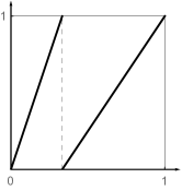
Figure 4.1. The endomorphism $\sigma^{\left(u\right)}$ from (4.4).

Definition 4.3.

An IFS $\left\{\tau_{j}\right\}_{j\in J}$ in $\left(X,\mathscr{B}\right)$, the given measure space, is said to be stable iff there is an endomorphism $\sigma$ in $\left(X,\mathscr{B}\right)$ such that

$$\sigma\circ\tau_{j}=id_{X},\;\forall j\in J.$$ (4.7)

Remark 4.4.

Suppose $\left(X,\mathscr{B},\left\{\tau_{j}\right\},\left\{p_{j}\right\}\right)$ is a stable IFS; set

$$\left(Rf\right)\left(x\right)=\sum_{j}p_{j}f\left(\tau_{j}\left(x\right)\right),\;x\in X,$$ (4.8)

then this transfer operator $R$ satisfies

$$R\left[\left(f\circ\sigma\right)g\right]=fR\left(g\right),\;\forall f,g\in\mathscr{F}\left(X,\mathscr{B}\right);$$ (4.9)

but in general (4.9) may not be satisfied for any choice of endomorphism $\sigma$.

4.2. IFSs: The measure category

We now return to the setting

$$G:X\times Y\longrightarrow X$$ (4.10)

from 3.3 where $\left(X,\mathscr{B}_{X}\right)$ and $\left(Y,\mathscr{B}_{Y}\right)$ are given measure spaces, $G$ in (4.10) is measurable from $X\times Y$ to $X$, and $X\times Y$ is given the product sigma-algebra.

We saw that for every choice of probability measure $\nu$ on $\left(Y,\mathscr{B}_{Y}\right)$, we get a corresponding transfer operator (3.3), depending on both $G$ and $\nu$. We further assume that $G\left(\cdot,y\right)$ is 1-1 on $X$, for $y\in Y$.

Theorem 4.5.

Let $G:X\times Y\rightarrow X$ be as in (4.10) for given measure spaces $\left(X,\mathscr{B}_{X}\right)$ and $\left(Y,\mathscr{B}_{Y}\right)$, let $\nu\in M_{1}\left(Y,\mathscr{B}_{Y}\right)$, and $\lambda\in M_{1}\left(X,\mathscr{B}_{X}\right)$ be fixed probability measures. Let $R=R_{\left(G,\nu\right)}$ be the corresponding transfer operator in $L^{2}\left(X,\lambda\right)$ given by

$$\left(Rf\right)\left(x\right)=\int_{Y}f\left(G\left(x,y\right)\right)d\nu\left(y\right),\;f\in\mathscr{F}\left(X,\mathscr{B}_{X}\right).$$ (4.11)

A given endomorphism $\sigma$ in $\left(X,\mathscr{B}_{X}\right)$ satisfies

$$R_{\left(G,\nu\right)}\left[\left(f_{1}\circ\sigma\right)f_{2}\right]=f_{1}R_{\left(G,\nu\right)}\left(f_{2}\right),\;\forall f_{1},f_{2}\in\mathscr{F}\left(X,\mathscr{B}_{X}\right)$$ (4.12)

if and only if

$$\sigma\left(G\left(x,y\right)\right)=x,$$ (4.13)

a.e. $y$ w.r.t. $\nu$, and a.e. $x$ w.r.t. $\lambda$.

Proof.

It is immediate that (4.13) $\Longrightarrow$ (4.12). Conversely suppose (4.12) holds. We then get

$$\int_{Y}f_{1}\left(\sigma\left(G\left(x,y\right)\right)\right)f_{2}\left(G\left(x,y\right)\right)d\nu\left(y\right)$$

$$= f_{1}\left(x\right)\int_{Y}f_{2}\left(G\left(x,y\right)\right)d\nu\left(y\right),$$

$\forall f_{1},f_{2}\in\mathscr{F}\left(X,\mathscr{B}_{X}\right)$, a.e. $x$ w.r.t. $\lambda$.

From the assumptions in the theorem, we conclude that the following identity holds for measures

$$\int\sigma\left(G\left(x,y\right)\right)d\nu\left(y\right)=\delta_{x},$$

a.e. $x$ (w.r.t. $\lambda$), and therefore

$$\sigma\left(G\left(x,y\right)\right)=x,$$

a.e. $y$ w.r.t. $\nu$, and a.e. $x$ w.r.t. $\lambda$, which is the desired conclusion (4.13). ∎

Remark 4.6.

It is easy to see that if $G$ is as in (3.8) in 3.6, then there is no solution $\sigma\in End\left(\left(0,1\right),\mathscr{B}\right)$ to the condition in (4.13); and so by the theorem; this particular IFS (in the generalized sense) is not stable in the sense of 4.3.

Definition 4.7.

Let $\left(X,\mathscr{B}_{X}\right)$, $\left(Y,\mathscr{B}_{Y}\right)$, $G$, and $\nu$ be as in the statement of 4.5. Let $R=R_{\left(G,\nu\right)}$ be the corresponding transfer operator, see (4.11).

Suppose $Y$ has the following factorization, $Y=U\times J$, where $\left(U,\mathscr{B}_{U}\right)$ is a measure space and $J$ is an at most countable index set. Let $\nu\left(\cdot\mid i\right)$, $i\in J$, be the induced conditional measures on $U$, i.e., for some $\left\{p_{j}\right\}_{j\in J}$ we have

$$\nu\left(\pi_{U}\in A,\>\pi_{J}=i\right)=p_{i}\nu\left(A\mid i\right)$$ (4.14)

for all $A\in\mathscr{B}_{U}$, $i\in J$, where

$$\pi_{U}\left(\left(u,i\right)\right)=u,\;\text{and }\pi_{J}\left(\left(u,i\right)\right)=i.$$ (4.15)

We say that the positive operator $R_{\left(G,\nu\right)}$ is decomposable if there is a representation $Y=U\times J$ with (4.14) such that, for $\nu\left(\cdot\mid i\right)$ a.e. $u\in U$, the induced IFS,

$$X\ni x\longmapsto G\left(x,u,i\right)$$ (4.16)

is stable (4.3); i.e., for $u$ fixed, $\exists\sigma^{\left(u\right)}\in End\left(X\right)$ such that

$$\sigma^{\left(u\right)}\left(G\left(x,\left(u,i\right)\right)\right)=x,\;\forall i\in J.$$ (4.17)

Theorem 4.8.

Let $\left(X,Y,G,\nu\right)$ be given as in the statement of 4.5; then the corresponding transfer operator $R=R_{\left(G,\nu\right)}$ is decomposable.

Proof.

This may be proved with the use of a Zorn lemma argument; see e.g., [Nel69]. (Details are left to the reader.) Note that the representation of $Y$ in (4.14)–(4.15) is not unique. ∎

Remark 4.9.

The reader will notice that the example from 3.6 (see (3.9)) is decomposable; see also 4.2.

Remark 4.10.

Return to the general case, let $R=R_{\left(G,\nu\right)}$ be given in its decomposable form with the measure $\nu$ represented as in (4.14) for a fixed system of weights $\left(p_{i}\right)_{i\in J}$, $\sum_{i}p_{i}=1$. Let $\left(\pi_{n}\right)_{n\in\mathbb{Z}_{+}\cup\left\{0\right\}}$be the corresponding Markov process on $\Omega_{X}=\prod_{0}^{\infty}X$; see 3.8. We then have the following formula for the Markov-move $\pi_{0}\rightarrow\pi_{1}$; and similarly for $\pi_{n}\rightarrow\pi_{n+1}$:

Let $x\in X$, and $A\in\mathscr{B}_{X}$, then

$$\mathbb{P}\left(\pi_{1}\in A\mid\pi_{0}=x\right)=\sum_{i\in J}p_{i}\int_{U}\nu\left(\left\{G\left(x,y\right)\in A\mid\pi_{U}\in du,\>\pi_{J}=i\right\}\right).$$ (4.18)

The Markov move is as follows: Step 1 selects $i$ with probability $p_{i}$, and the second step selects $\pi_{1}\in A$ from $\nu\left(\cdot\mid i\right)$; see 4.2.

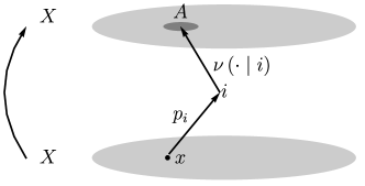
Figure 4.2. The Markov-move $\pi_{0}\rightarrow\pi_{1}$, see (4.18).

5. Generalized multiresolutions associated to measure spaces with endomorphism

5.1. Multiresolutions

In this section we introduce the aforementioned multiresolutions, with the scale of resolution subspaces referring to the Hilbert spaces $L^{2}\left(\Omega,\mathbb{P}\right)$ of square integrable random variables.

In classical wavelet theory, the accepted use is instead the Hilbert space $L^{2}\left(\mathbb{R}\right)$, and systems of functions $\varphi$, $\left(\psi_{i}\right)$ in $L^{2}\left(\mathbb{R}\right)$ such that

$$\varphi\left(x\right) =\sqrt{N}\sum_{k\in\mathbb{Z}}a_{k}\varphi\left(Nx-k\right),\;\text{and}$$ (5.1)

$$\psi_{i}\left(x\right) =\sqrt{N}\sum_{k\in\mathbb{Z}}b_{k}^{\left(i\right)}\varphi\left(Nx-k\right)$$ (5.2)

where the coefficients $\left(a_{k}\right)$ and $\left(b_{k}^{\left(i\right)}\right)$ are called wavelet masking coefficients. From this one creates wavelet multiresolutions as follows:

1. $\mathscr{H}_{n}$, $\mathscr{H}_{n}\subset\mathscr{H}_{n+1}$, $\land_{n}\mathscr{H}_{n}=\left\{0\right\}$, $\lor_{n}\mathscr{H}_{n}=L^{2}\left(\mathbb{R}\right)$;

2. $\mathscr{H}_{0}=\lor span\left\{\varphi\left(\cdot-k\right)\mid k\in\mathbb{Z}\right\}$;

3. $\exists N\in\mathbb{N}$, $N>1$, such that $\mathscr{H}_{0}\ominus\mathscr{H}_{1}=\lor\left\{\psi_{j}\left(\cdot-k\right)\mid 1\leq j<N,k\in\mathbb{Z}\right\}$;

4. $U^{k}\mathscr{H}_{0}=\mathscr{H}_{-k}$, $k\in\mathbb{Z}$, where

   $$\left(Uf\right)\left(x\right)=\frac{1}{\sqrt{N}}f\left(\frac{x}{N}\right).$$ (5.3)

So if $N>1$ is fixed, the goal is the construction of functions $\psi_{1},\psi_{2},\cdots,\psi_{N-1}$ such that the corresponding triple-indexed family

$$\psi_{j,k,n}\left(x\right)= N^{\frac{n}{2}}\psi_{j}\left(N^{n}x-k\right),$$

$$j=1,\cdots,N-1,\>k,n\in\mathbb{Z},$$ (5.4)

forms a suitable frame in $L^{2}\left(\mathbb{R}\right)$; or even an ONB.

For more details, see [Dau92, BJ02a, WTLW16, Wan16, JT15, DJ14].

Definition 5.1.

Let $\left(\Omega,\mathscr{F},\mathbb{P}\right)$ be a probability space, and let $\mathscr{A}\subset\mathscr{F}$ be a sub-sigma algebra. For every $\xi\in L^{2}\left(\Omega,\mathscr{F},\mathbb{P}\right)$ we define the conditional expectation $\mathbb{E}\left(\xi\mid\mathscr{A}\right)$ as the Radon-Nikodym derivative

$$\mathbb{E}\left(\xi\mid\mathscr{A}\right):=\frac{d\left(\xi d\mathbb{P}\right)}{d\mathbb{P}\big{|}_{\mathscr{A}}}.$$ (5.5)

Note further that $\mathbb{E}\left(\cdot\mid\mathscr{A}\right)$ is the orthogonal projection of $L^{2}\left(\Omega,\mathscr{F},\mathbb{P}\right)$ onto the closed subspace $L^{2}\left(\Omega,\mathscr{A},\mathbb{P}\big{|}_{\mathscr{A}}\right)$; i.e., we have

$$\int_{\Omega}\varphi\,\xi\,d\mathbb{P}=\int_{\Omega}\varphi\,\mathbb{E}\left(\xi\mid\mathscr{A}\right)d\mathbb{P}$$

for all $\varphi$ $\mathscr{A}$-measurable, and all $\xi\in L^{2}\left(\Omega,\mathscr{F},\mathbb{P}\right)$.

In our applications below we shall consider multiresolutions $\mathscr{H}_{n}\subset L^{2}\left(\Omega,\mathscr{F},\mathbb{P}\right)$ which result from filtrations $\mathscr{F}_{n}\subset\mathscr{F}$ s.t. $\mathscr{F}_{n}\subset\mathscr{F}_{n+1}$, $\bigwedge_{n}\mathscr{F}_{n}=\left\{\emptyset,X\right\}$ mod sets of $\mathbb{P}$-measure zero; and $\bigvee_{n}\mathscr{F}_{n}=\mathscr{F}$. For every filtration, we shall consider the corresponding conditional expectations $\mathbb{E}\left(\cdot\mid\mathscr{F}_{n}\right):=\mathbb{E}_{n}\left(\cdot\right)$.

5.2. Wavelet resolutions (review)

We shall be interested in multiresolutions, both for the standard $L^{2}\left(\mathbb{R}^{d}\right)$ Hilbert spaces, and for the $L^{2}$ Hilbert spaces formed from those probability spaces $\left(\Omega,\mathscr{F},\mathbb{P}\right)$ we discussed in 3. To help draw parallels we begin with $L^{2}\left(\mathbb{R}^{d}\right)$. In both cases, the construction takes as starting point certain Ruelle transfer operators.

In its simplest form, a wavelet is a function $\psi$ on the real line $\mathbb{R}$ such that the doubly indexed family $\left\{2^{n/2}\psi\left(2^{n}x-k\right)\right\}_{n,k\in\mathbb{Z}}$ provides a basis or frame for all the functions in a suitable space such as $L^{2}\left(\mathbb{R}\right)$. (Below, we specialize to the case $N=2$ for simplicity, see (5.3)-(5.4).) Since $L^{2}\left(\mathbb{R}\right)$ comes with a norm and inner product, it is natural to ask that the basis functions be normalized and mutually orthogonal (but many useful wavelets are not orthogonal). The analog-to-digital problem from signal processing (see e.g., [WTLW16, KGEW16]) concerns the correspondence

$$f\left(x\right)\longleftrightarrow c_{n,k}$$ (5.6)

for the wavelet representation

$$f\left(x\right)=\sum_{n\in\mathbb{Z}}\sum_{k\in\mathbb{Z}}c_{n,k}2^{n/2}\psi\left(2^{n}x-k\right).$$ (5.7)

We will be working primarily with the Hilbert space $L^{2}\left(\mathbb{R}\right)$, and we allow complex-valued functions. Hence the inner product $\left\langle f,g\right\rangle=\int\overline{f\left(x\right)}g\left(x\right)dx$ has a complex conjugate on the first factor in the product under the integral sign. If $f$ represents a signal in analog form, the wavelet coefficients $c_{n,k}$ offer a digital representation of the signal, and the correspondence between the two sides in (5.6) is a new form of the analysis/synthesis problem, quite analogous to Fourier’s analysis/synthesis problem of classical mathematics (see e.g., [BJMP05, AYB15, DSKL14]). One reason for the success of wavelets is the fact that the algorithms for the problem (5.6) are faster than the classical ones in the context of Fourier.

Nonetheless, classical wavelet multiresolutions have the following limitation: Unless the wavelet filter (in the form of a multi-band matrix valued frequency function) under consideration satisfies some strong restriction, the Hilbert space $L^{2}\left(\mathbb{R}^{d}\right)$ is not a receptacle for realization. In other words, the resolution subspaces sketched in 5.1 cannot be realized as subspaces in the standard $L^{2}\left(\mathbb{R}^{d}\right)$-space; rather we must resort to a probability space built on a solenoid. The latter is related to $\mathbb{R}^{d}$, but different: As we outline in the remaining of our paper, it may be built from the same scaling which is used in the classical case (see (5.10) for the special case of $d=1$), only, in the more general setting, we must instead use a “bigger” Hilbert space; see 5.15 below for details. Using ideas from [Jor04] it is possible to show that $\mathbb{R}^{d}$ will be embedded inside the corresponding solenoid; see also [BJ02b, DJ06b, DJ14, Jor04, JS12a, DJ06a, Jor05, DJ05]. For related results, see [FGKP16, LP13, BMPR12].

The wavelet algorithms can be cast geometrically in terms of subspaces in Hilbert space which describe a scale of resolutions of some signal or some picture. They are tailor-made for an algorithmic approach that is based upon unitary matrices or upon functions with values in the unitary matrices. Wavelet analysis takes place in some Hilbert space $\mathscr{H}$ of functions on $\mathbb{R}^{d}$, for example, $\mathscr{H}=L^{2}\left(\mathbb{R}^{d}\right)$. An indexed family of closed subspaces $\left\{\mathcal{V}_{n}\right\}_{-\infty<n<\infty}$ such that

$$\mathcal{V}_{n} \subset\mathcal{V}_{n+1},\;U\mathcal{V}_{n+1}\subset\mathcal{V}_{n},\;\bigcap_{n\in\mathbb{Z}}\mathcal{V}_{n}=\left\{0\right\},\;\text{and}$$

$$\bigvee_{n\in\mathbb{Z}}\mathcal{V}_{n}=L^{2}\left(\mathbb{R}^{d}\right),\;\text{see Fig \ref{fig:gmw1} and \ref{fig:gmw2},}$$ (5.8)

is said to offer a resolution. (To stress the variety of spaces in this telescoping family, we often use the word multiresolution.) Here the symbol $\bigvee$ denotes the closed linear span. In pictures, the configuration of subspaces looks like 5.1.

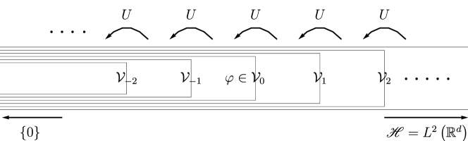
Figure 5.1. The subspaces of a resolution.

When shopping for a digital camera: just as important as the resolutions themselves (as given here by the scale of closed subspaces $\mathcal{V}_{n}$) are the associated spaces of detail. (See 5.3 below.) As expected, the details of a signal represent the relative complements between the two resolutions, a coarser one and a more refined one.

Starting with the Hilbert-space approach to signals, we are led to the following closed subspaces (relative orthogonal complements):

$$\mathcal{W}_{n}:= \mathcal{V}_{n+1}\ominus\mathcal{V}_{n}$$ (5.9)

$$= \left\{f\in\mathcal{V}_{n}\>:\>\left\langle f,h\right\rangle=0,\>h\in\mathcal{V}_{n}\right\},$$

and the signals in these intermediate spaces $\mathcal{W}_{n}$ then constitute the amount of detail which must be added to the resolution $\mathcal{V}_{n}$ in order to arrive at the next refinement $\mathcal{V}_{n+1}$. In 5.2, the intermediate spaces $\mathcal{W}_{n}$ of (5.9) represent incremental details in the resolution. See also [JS07, JS12a, JS12b, DPS14].

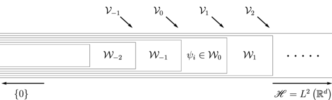
Figure 5.2. Incremental Detail.

The simplest instance of this is the one which Haar discovered in 1910 [Haa10] for $L^{2}\left(\mathbb{R}\right)$. There, for each $n\in\mathbb{Z}$, $\mathcal{V}_{n}$ represents the space of all step functions with step size $2^{-n}$, i.e., the functions $f$ on $\mathbb{R}$ which are constant in each of the dyadic intervals $j2^{-n}\leq x<\left(j+1\right)2^{-n}$, $j=0,\ldots,2^{n}-1$, and their integral translates, and which satisfy $\left\|f\right\|^{2}=\int_{-\infty}^{\infty}\left|f\left(x\right)\right|^{2}dx<\infty$.

Figure 5.3. A coarser resolution in three directions in the plane, filtering in directions, $x,y$, and diagonal; — corresponding dyadic scaling in each coordinate direction. (Image cited from M.-S. Song, “Wavelet Image Compression” in [HJL06].)

An operator $U$ in a Hilbert space is unitary if it is onto and preserves the norm or, equivalently, the inner product. Unitary operators are invertible, and $U^{-1}=U^{*}$ where the $*$ refers to the adjoint. Similarly, the orthogonality property for a projection $P$ in a Hilbert space may be stated purely algebraically as $P=P^{2}=P^{*}$. The adjoint $*$ is also familiar from matrix theory, where $\left(A^{*}\right)_{i,j}=\overline{A_{j,i}}$: in words, the $*$ refers to the operation of transposing and taking the complex conjugate. In the matrix case, the norm on $\mathbb{C}^{n}$ is $(\sum_{k}\left|x_{k}\right|^{2})^{1/2}$. In infinite dimensions, there are isometries which map the Hilbert space into a proper subspace of itself.

For Haar’s case we can scale between the resolutions using $f\left(x\right)\mapsto f\left(x/2\right)$, which represents a dyadic scaling.

To make it unitary, take

$$U=U_{2}:f\longmapsto 2^{-\frac{1}{2}}f\left(\frac{x}{2}\right),$$ (5.10)

which maps each space $\mathcal{V}_{n}$ onto the next coarser subspace $\mathcal{V}_{n-1}$, and $\left\|Uf\right\|=\left\|f\right\|$, $f\in L^{2}\left(\mathbb{R}\right)$. This can be stated geometrically, using the respective orthogonal projections $P_{n}$ onto the resolution spaces $\mathcal{V}_{n}$, as the identity

$$UP_{n}U^{-1}=P_{n-1}.$$ (5.11)

And (5.11) is a basic geometric reflection of a self-similarity feature of the cascades of wavelet approximations (see e.g., [BJ02a, Dau92, Jor99, Jor04, KFB16]). It is made intuitively clear in Haar’s simple but illuminating example. The important fact is that this geometric self-similarity, in the form of (5.11), holds completely generally. See Sections 5.3, 6 and 12 below.

5.3. Multiresolutions in $L^{2}\left(\Omega,\mathscr{C},\mathbb{P}\right)$

Here we aim to realize multiresolutions in probability spaces $\left(\Omega,\mathscr{F},\mathbb{P}\right)$; and we now proceed to outline the details.

We first need some preliminary facts and lemmas.

Lemma 5.2.

Let $\left(\Omega,\mathscr{F},\mathbb{P}\right)$ be a probability space, and let $A:\Omega\rightarrow X$ be a random variable with values in a fixed measure space $\left(X,\mathscr{B}_{X}\right)$, then $V_{A}f:=f\circ A$ defines an isometry $L^{2}\left(X,\mu_{A}\right)\rightarrow L^{2}\left(\Omega,\mathbb{P}\right)$ where $\mu_{A}$ is the law (distribution) of $A$, i.e., $\mu_{A}\left(\Delta\right):=\mathbb{P}\left(A^{-1}\left(\Delta\right)\right)$, $\forall\Delta\in\mathscr{B}_{X}$; and $V_{A}^{*}\left(\psi\right)\left(x\right)=\mathbb{E}_{\left\{A=x\right\}}\left(\psi\mid\mathscr{F}_{A}\right)$, for all $\psi\in L^{2}\left(\Omega,\mathbb{P}\right)$, and all $x\in X$.

We shall apply 5.2 to the case when $\left(\Omega,\mathscr{F},\mathbb{P}\right)$ is realized on an infinite product space as follows:

Definition 5.3.

Let $\left(\Omega_{X},\mathscr{F},\mathbb{P}\right)$ be a probability space, where $\Omega_{X}=\prod_{n=0}^{\infty}X$. Let $\pi_{n}:\Omega_{X}\rightarrow X$ be the random variables given by

$$\pi_{n}\left(x_{0},x_{1},x_{2},\cdots\right)=x_{n},\;\forall n\in\mathbb{N}_{0}.$$ (5.12)

The sigma-algebra generated by $\pi_{n}$ will be denoted $\mathscr{F}_{n}$, and the isometry corresponding to $\pi_{n}$ will be denoted $V_{n}$.

Remark 5.4.

Suppose the measure space $\left(X,\mathscr{B}_{X}\right)$ in 5.2 is specialized to $\left(\mathbb{R},\mathscr{B}\right)$; it is then natural to consider Gaussian probability spaces $\left(\Omega,\mathscr{F},\mathbb{P}\right)$ where $\Omega$ is a suitable choice of sample space, and $A:\Omega\rightarrow X$ is replaced with Brownian motion $B_{t}:\Omega\rightarrow\mathbb{R}$, see [Hid80, Hid90, AØ15, AK15]. We instead consider samples

$$0<t_{1}<t_{2}<\cdots<t_{n},$$

and functions $F$ on $\mathbb{R}^{n}$ with now $f\rightarrow f\circ A$ replaced with a suitable Malliavin derivative

$$DF_{n}\left(B_{\varphi_{1}},\cdots,B_{\varphi_{n}}\right)=\sum_{i=1}^{n}\frac{\partial F_{n}}{\partial x_{i}}\left(B_{\varphi_{1}},\cdots,B_{\varphi_{n}}\right)\varphi_{i},$$ (5.13)

where $B_{\varphi}=\int\varphi\left(t\right)dB_{t}$.

We computed the adjoint of (5.13) in [JT16] and identified it as a multiple Ito-integral. For more details, we refer the reader to the papers [BNBS14, HRZ14, AH84, HPP00, CH13], and also see [Bog98, HKPS13].

Definition 5.5.

Let $R$ be a positive transfer operator, i.e., $f\geq 0\Rightarrow Rf\geq 0$, $R\mathbbm{1}=\mathbbm{1}$ (see 2), let $\lambda$ be a probability measure on a fixed measure space $\left(X,\mathscr{B}_{X}\right)$. We further assume that

$$R\left(\left(f\circ\sigma\right)g\right)=fR\left(g\right),\;\forall f,g\in\mathscr{F}\left(X,\mathscr{B}_{X}\right).$$ (5.14)

Denote $\mu\left(\cdot\mid x\right)$, $x\in X$, the conditional measures determined by

$$Rf\left(x\right)=\int_{X}f\left(y\right)\mu\left(dy\mid x\right),$$ (5.15)

for all $f\in C\left(X\right)$, representing $R$ as an integral operator. Set

$$\mu\left(B\mid x\right):= R\left(\chi_{B}\right)\left(x\right),\;\forall B\in\mathscr{B}_{X}$$

$$= \mathbb{P}\left(\pi_{1}\in B\mid\pi_{0}=x\right).$$ (5.16)

Note the RHS of (5.15) extends to all measurable functions on $X$, and we shall write $R$ also for this extension.

Lemma 5.6.

Let $\left\{\mu\left(\cdot\mid x\right)\right\}_{x\in X}$ be as in (5.15), and $W:=\frac{d\lambda R}{d\lambda}=$ Radon-Nikodym derivative. If $B\in\mathscr{B}_{X}$ then

$$\int_{X}\mu\left(B\mid x\right)d\lambda\left(x\right)=\int_{B}W\left(x\right)d\lambda\left(x\right).$$

Proof.

Let $B\in\mathscr{B}_{X}$, then

LHS $$=\int_{X}R\left(\chi_{B}\right)\left(x\right)d\lambda\left(x\right)$$

$$=\int_{X}\chi_{B}d\left(\lambda R\right)=\int_{B}W\left(x\right)d\lambda\left(x\right)=\text{RHS}.$$

∎

Lemma 5.7.

Suppose $R$ has a representation

$$R\left(\chi_{B}\right)\left(x\right)=\mu\left(B\mid x\right),\;B\in\mathscr{B}_{X},\;x\in X.$$

Then the following are equivalent:

1. $R\left[\left(f\circ\sigma\right)g\right]\left(x\right)=f\left(x\right)R\left(g\right)\left(x\right)$, $\forall x\in X$, $\forall f,g\in\mathscr{F}\left(X,\mathscr{B}\right)$;

2. $\mu\left(\sigma^{-1}\left(A\right)\cap B\mid x\right)=\chi_{A}\left(x\right)\mu\left(B\mid x\right)$, $\forall A,B\in\mathscr{B}$, $\forall x\in X$.

Proof.

Recall that, by assumption, $\left(Rf\right)\left(x\right)=\int_{X}f\left(x\right)\mu\left(dy\mid x\right)$. The conclusion follows by setting $f=\chi_{A}$, and $g=\chi_{B}$. ∎

Proposition 5.8.

Let $\left\{\mu\left(\cdot\mid x\right)\right\}_{x\in X}$ be the Markov process indexed by $x\in X$ (see (5.15)), where $\left(X,\mathscr{B}_{X}\right)$ is a fixed measure space, and let $\mathbb{P}$ be the corresponding path space measure (see, e.g., [CFS82, HKPS13]) determined by (3.13)-(3.14). Let $\sigma\in End\left(X,\mathscr{B}_{X}\right)$ as in Def. 3.2. Then

$$\text{suppt}\left(\mathbb{P}\right) \subset Sol_{\sigma}\left(X\right)$$

$$\Updownarrow$$ (5.17)

$$\mathbb{P}\left(\pi_{k+1}\in B\cap\sigma^{-1}\left(A\right)\mid\pi_{k}=x\right) =\chi_{A}\left(x\right)\mathbb{P}\left(\pi_{k+1}\in B\mid\pi_{k}=x\right).$$

The next result will serve as a tool in our subsequent study of multiresolutions, orthogonality relations, and scale-similarity, each induced by a given endomorphism; the theme to be studied in detail in 12 below.

Theorem 5.9.

Let $\left(X,\sigma,R,h,\lambda,W\right)$ be as above, $W=\frac{d\lambda R}{d\lambda}$; then

1. $\exists!$ path space measure $\mathbb{P}$ on $Sol_{\sigma}\left(X\right)$, such that

   $$L^{2}\left(X,\mu_{n}\right)\xrightarrow{\;V_{n}\;}L^{2}\left(Sol_{\sigma},\mathbb{P}\right),\;V_{n}f=f\circ\pi_{n}$$ (5.18)

   is isometric, where $\mu_{n}:=\text{dist}\left(\pi_{n}\right)$, and $\int_{X}f\,d\mu_{n}=\int_{X}R^{n}\left(fh\right)d\lambda$;

2. $\mathbb{P}$ has the property:

   $$\frac{d\mathbb{P}\circ\tilde{\sigma}}{d\mathbb{P}}=W\circ\pi_{0},$$ (5.19)

   where $\tilde{\sigma}$ is as in (3.2).

Proof.

See [JT15, DJ14]. ∎

Lemma 5.10.

Let $\Omega_{X}$, $\mathscr{F}$, $\mathbb{P}$, $R$, $h$, $\lambda$ be as above, assume $R\mathbbm{1}=\mathbbm{1}$. Let $V_{n}:L^{2}\left(X,\mu_{n}\right)\rightarrow L^{2}\left(Sol_{\sigma},\mathbb{P}\right)$ be the isometry in (5.18) (also see 5.3). Then $V_{n}V_{n}^{*}$ is a projection in $L^{2}\left(Sol_{\sigma},\mathbb{P}\right)$, and it is the conditional expectation on $\mathscr{H}_{n}$, i.e.,

$$V_{n}V_{n}^{*}\psi=\mathbb{E}\left(\psi\mid\mathscr{F}_{n}\right),\;\forall\psi\in L^{2}\left(Sol_{\sigma},\mathbb{P}\right).$$ (5.20)

Moreover,

$$\mathbb{E}\left(\psi\mid\mathscr{F}_{n}\right)=\left(V_{n}^{*}\psi\right)\circ\pi_{n}\xrightarrow[\;n\rightarrow\infty\;]{}\psi,$$ (5.21)

i.e.,

$$\left\|\psi-\left(V_{n}^{*}\psi\right)\circ\pi_{n}\right\|_{L^{2}\left(\mathbb{P}\right)}\xrightarrow[\;n\rightarrow\infty\;]{\text{in norm}}0.$$

In order to get an orthogonal decomposition relative to the detail spaces

$$\mathscr{D}_{n}=\mathscr{H}_{n}\ominus\mathscr{H}_{n-1}=\left\{\psi\in\mathscr{H}_{n}\mid\psi\perp\mathscr{H}_{n-1}\right\},$$ (5.22)

we shall use that

$$\mathbb{E}\left(\cdot\mid\mathscr{F}_{n}\right)= \text{the orthogonal projection in }L^{2}\left(Sol_{\sigma},\mathbb{P}\right)$$ (5.23)

$$\text{onto }\mathscr{H}_{n},$$

and so the orthogonal projection onto $\mathscr{D}_{n}$ is

$$\mathbb{E}\left(\cdot\mid\mathscr{F}_{n}\right)-\mathbb{E}\left(\cdot\mid\mathscr{F}_{n-1}\right).$$ (5.24)

Lemma 5.11.

Assume $R\mathbbm{1}=\mathbbm{1}$. For all $f\in\mathscr{F}\left(X,\mathscr{B}_{X}\right)$, we have

$$VV^{*}\left(f\circ\pi_{n+k}\right)=\left[R^{k}\left(f\right)-R^{k+1}\left(f\right)\circ\sigma\right]\circ\pi_{n}.$$ (5.25)

Proof.

Note that, for all $f,g\in\mathscr{F}\left(X,\mathscr{B}_{X}\right)$,

$$\int_{Sol_{\sigma}}\left(g\circ\pi_{n}\right)\left(f\circ\pi_{n+k}\right)d\mathbb{P}$$

$$= \int_{Sol_{\sigma}}\left(\left(g\circ\sigma^{k}\right)f\right)\circ\pi_{n+k}d\mathbb{P}=\int_{X}R^{n+k}\left(\left(g\circ\sigma^{k}\right)f\right)h\,d\lambda$$

$$= \int_{X}R^{n}\left(gR^{k}\left(f\right)\right)h\,d\lambda=\int_{Sol_{\sigma}}\left(g\circ\pi_{n}\right)\left(R^{k}\left(f\right)\circ\pi_{n}\right)d\mathbb{P},$$

and so $\mathbb{E}\left(f\circ\pi_{n+k}\mid\mathscr{F}_{n}\right)=R^{k}\left(f\right)\circ\pi_{n}$.

Apply (5.24) to $f\circ\pi_{n+k}$, then

$$\mathbb{E}\left(f\circ\pi_{n+k}\mid\mathscr{F}_{n}\right)-\mathbb{E}\left(f\circ\pi_{n+k}\mid\mathscr{F}_{n-1}\right)$$

$$= R^{k}\left(f\right)\circ\pi_{n}-R^{k+1}\left(f\right)\circ\pi_{n-1}$$

$$= \left[R^{k}\left(f\right)-R^{k+1}\left(f\right)\circ\sigma\right]\circ\pi_{n},$$

which is assertion. ∎

Lemma 5.12.

Assume $R\mathbbm{1}=\mathbbm{1}$, then

$$R\left[f-R\left(f\right)\circ\sigma\right]\equiv 0,\;\forall f\in\mathscr{F}\left(X,\mathscr{B}_{X}\right).$$

Proof.

It follows from (5.14) that

$$R\left(R\left(f\right)\circ\sigma\right)=R\left(R\left(f\right)\circ\sigma\mathbbm{1}\right)=R\left(f\right)R\left(\mathbbm{1}\right)=R\left(f\right).$$

∎

Remark 5.13.

The path space measure from (3.13) (see, e.g., [CFS82, HKPS13]) can be formulated as follows:

Assume $R^{\prime}\mathbbm{1}=\mathbbm{1}$, and $\int_{X}h\,d\lambda=1$, and let $\mathbb{P}$ be determined by

$$\int_{\Omega_{X}}\left(f_{0}\circ\pi_{0}\right)\left(f_{1}\circ\pi_{1}\right)\cdots\left(f_{n}\circ\pi_{n}\right)d\mathbb{P}$$

$$= \int_{X}f_{0}\left(x\right)R^{\prime}\left(f_{1}R\left(f_{2}\cdots R^{\prime}\left(f_{n}\right)\right)\cdots\right)\left(x\right)h\left(x\right)d\lambda\left(x\right).$$ (5.26)

The two constructions in (3.13) and (5.26) are equivalent and generate the same path space measure. See 5.14 below.

5.4. Renormalization

The purpose of the next result is to show that in the study of path-space measures associated to positive transfer operators $R$ one may in fact reduce to the case when $R$ is assumed normalized; see (5.27) in the statement of the theorem. The result will be used in the remaining of our paper.

Theorem 5.14.

Let $\left(X,\mathscr{B}_{X},R,h,\lambda\right)$ be as above, i.e., $Rh=h$, $h\geq 0$, $\int_{X}h\,d\lambda=1$, and let $\mathbb{P}$ be the corresponding probability measure on $\Omega_{X}=\prod_{n=0}^{\infty}\left(X,\mathscr{B}_{X}\right)$ equipped with its cylinder sigma-algebra $\mathscr{C}$.

Define $R^{\prime}$ as follows:

$$R^{\prime}\left(f\right):=\frac{R\left(fh\right)}{h},\;\forall f\in\mathscr{F}\left(X,\mathscr{B}_{X}\right),$$ (5.27)

then $R^{\prime}$ is well defined, $R^{\prime}\left(\mathbbm{1}\right)=\mathbbm{1}$, and $\left(R^{\prime},\lambda\right)$ generates the same probability space $\left(\Omega_{X},\mathscr{C},\mathbb{P}\right)$. (See also 5.13.)

Proof.

To see that $R^{\prime}$ (in (5.27)) is well defined, note that a repeated application of Schwarz yields:

$$\left|R\left(fh\right)\right|\leq\left(R\left(f^{2}h\right)\right)^{\frac{1}{2}}h^{\frac{1}{2}}\leq\cdots\leq R\left(f^{2^{n}}h\right)^{\frac{1}{2^{n}}}h^{\frac{1}{2}+\cdots+\frac{1}{2^{n}}}$$

for all $f\in\mathscr{F}\left(X,\mathscr{B}_{X}\right)$, and all $n\in\mathbb{N}$.

For each $n\in\mathbb{Z}_{+}$, consider $f_{0},f_{1},\cdots,f_{n}$ in $\mathscr{F}\left(X,\mathscr{B}_{X}\right)$. We note that $\mathbb{P}$ from $\left(R,h,\lambda\right)$ is determined by the conditional measures

$$\int_{\Omega_{X}}\left(f_{0}\circ\pi_{0}\right)\left(f_{1}\circ\pi_{1}\right)\cdots\left(f_{n}\circ\pi_{n}\right)d\mathbb{P}$$

$$= \int_{X}f_{0}\left(x\right)R\left(f_{1}R\left(f_{2}\cdots R\left(f_{n}h\right)\cdots\right)\right)\left(x\right)d\lambda\left(x\right),\;\text{and}$$ (5.28)

$$\int_{\Omega_{X}}\left(f\circ\pi_{0}\right)d\mathbb{P}=\int_{X}f\,h\,d\lambda,$$

while the measures on $\left(\Omega_{X},\mathscr{C}\right)$ determined by $R^{\prime}$ from (5.27) are

$$\int_{X}f_{0}\left(x\right)R^{\prime}\left(f_{1}R^{\prime}\left(f_{2}\cdots R^{\prime}\left(f_{n}\right)\cdots\right)\right)\left(x\right)h\left(x\right)d\lambda\left(x\right).$$ (5.29)

But an induction by $n$ shows that the integrals in (5.29) agree with the RHS in (5.28) for all $n\in\mathbb{N}$, and all $f_{0},f_{1},\cdots,f_{n}$ in $\mathscr{F}\left(X,\mathscr{B}_{X}\right)$. We then conclude from Kolmogorov consistency that the two measures on $\left(\Omega_{X},\mathscr{C}\right)$ agree; i.e., that $\left(R,h,\lambda\right)$ and $\left(R^{\prime},\mathbbm{1},h\,d\lambda\right)$ induce the same path space measure on $\left(\Omega_{X},\mathscr{C}\right)$, i.e., we get the same $\mathbb{P}$ for the unnormalized $R$ as from its normalized counterpart. See, e.g., [Hid80, Moh14, SSBR71]. ∎

Theorem 5.15.

Let $\Omega_{X}$, $\mathscr{F}$, $\mathbb{P}$, $R$, $h$, $\lambda$ be as specified above, such that $R\mathbbm{1}=\mathbbm{1}$, and $\mathbb{P}$ is determined by (5.26). Set

$$\mathscr{H}_{n}:=\bigvee\left\{f\circ\pi_{n}\mid f\in L^{2}\left(X,\mathscr{B}_{X},\lambda\right)\right\}.$$

Let $\sigma:X\rightarrow X$ be a measurable endomorphism mapping $X$ onto itself. Assume further that

1. $\bigcap_{n=1}^{\infty}\sigma^{-n}\left(\mathscr{B}_{X}\right)=\left\{\emptyset,X\right\}$ mod sets of $\lambda$-measure zero;

2. $R\left(\left(f\circ\sigma\right)g\right)=fR\left(g\right)$, $\forall f,g\in\mathscr{F}\left(X,\mathscr{B}_{X}\right)$.

Then the resolution space $\mathscr{H}_{n}$ has an orthogonal decomposition in $L^{2}\left(Sol_{\sigma},\mathbb{P}\right)$ as follows (5.4): Setting

$$\mathscr{D}_{k}=\mathscr{H}_{k}\ominus\mathscr{H}_{k-1}\left(=\text{detail subspace}\right),\;k=1,\cdots,n;$$ (5.30)

then

$$f\circ\pi_{n}=\underset{\in\mathscr{D}_{n}}{\underbrace{\left(f-R\left(f\right)\circ\sigma\right)\circ\pi_{n}}}+\underset{\in\mathscr{D}_{n-1}}{\underbrace{\left(R\left(f\right)-R^{2}\left(f\right)\circ\sigma\right)\circ\pi_{n-1}}}+\cdots$$ (5.31)

is the corresponding orthogonal decomposition for arbitrary vectors in the $n^{th}$ resolution subspace in $L^{2}\left(Sol_{\sigma},\mathbb{P}\right)$.

Proof.

Note that

$$\int_{Sol_{\sigma}}\left(g\circ\pi_{n-1}\right)\left(f-R\left(f\right)\circ\sigma\right)\circ\pi_{n}d\mathbb{P}$$

$$= \int_{Sol_{\sigma}}\left(g\circ\pi_{n-1}\right)\left(f\circ\pi_{n}\right)d\mathbb{P}-\int_{Sol_{\sigma}}\left(g\circ\pi_{n-1}\right)R\left(f\right)\circ\underset{\pi_{n-1}}{\underbrace{\sigma\circ\pi_{n}}}d\mathbb{P}$$

$$= \int_{X}R^{n-1}\left(gR\left(f\right)\right)h\,d\lambda-\int_{X}R^{n-1}\left(gR\left(f\right)\right)h\,d\lambda=0,\;\forall f,g\in\mathscr{F}\left(X,\mathscr{B}_{X}\right),$$

and the conclusion follows by induction. Also see 5.11. ∎

Figure 5.4.

Example 5.16.

For $f\in\mathscr{F}\left(X,\mathscr{B}_{X}\right)$, apply (5.31) to $f\circ\pi_{1}$ then

$$f\circ\pi_{1}=\left(f-R\left(f\right)\circ\sigma\right)\circ\pi_{1}+R\left(f\right)\circ\pi_{0},$$

and by Parseval’s identity,

$$\int_{X}R\left(f^{2}\right)hd\lambda=\int_{X}\left(R\left(f^{2}\right)-R\left(f\right)^{2}\right)h\,d\lambda+\int_{X}R\left(f\right)^{2}h\,d\lambda.$$

Remark 5.17 (Analogy with Brownian motion).

Let $\left(B_{t}\right)_{t\in\left[0,T\right]}$ be the standard Brownian motion, so that $\mathbb{E}\left(B_{s}B_{t}\right)=s\wedge t=\min\left(s,t\right)$, then

$$\mathbb{E}\left(\left|\int_{0}^{T}f\left(B_{t}\right)dB_{t}\right|^{2}\mid\mathscr{F}_{0}\right)=\int_{0}^{T}\left|f\left(t\right)\right|^{2}dt.$$

Note that in our current setting, we have

$$\mathbb{E}\left(f^{2}\circ\pi_{n}\mid\mathscr{F}_{0}\right) =\int_{X}\left|f\right|^{2}d\mu_{n}$$

$$=\sum_{k=0}^{n}\int_{X}R^{k}\left(R\left(f^{2}\right)-R\left(f\right)^{2}\right)d\lambda.$$

Also see [Hid80, Hid85, AØ15, AK15].

Lemma 5.18.

For all $f\in L^{\infty}\left(X,\mathscr{B}_{X},\lambda\right)$, let $\rho\left(f\right):=$ multiplication by $f\circ\pi_{0}$, as an operator in $L^{2}\left(\Omega_{X},\mathscr{F},\mathbb{P}\right)$, then the action of $\left\{\rho\left(f\right)\right\}_{f\in L^{2}\left(X\right)}$ is as follows:

Every subspace $\mathscr{H}_{n}$ is invariant under $\rho\left(f\right)$,where

$$\rho\left(f\right)\big{|}_{\mathscr{H}_{n}} =M_{f\circ\sigma^{n}}=\text{multiplication by }f\circ\sigma^{n}$$ (5.32)

$$\rho\left(f\right)\big{|}_{\mathscr{D}_{n}} =0,\quad\mathscr{D}_{n}:=\mathscr{H}_{n}\ominus\mathscr{H}_{n-1}.$$ (5.33)

Proof.

(Sketch) Note that

$$\rho\left(f\right)g\circ\pi_{n}=\left(f\circ\pi_{0}\right)\left(g\circ\pi_{n}\right)=\left(\left(f\circ\sigma^{n}\right)g\right)\circ\pi_{n}.$$

The conclusion follows from this. ∎

6. Unitary scaling in $L^{2}\left(\Omega,\mathscr{C},\mathbb{P}\right)$

Let $\left(X,\mathscr{B}\right)$ be a measure space, and let $R$ be a positive operator in $\mathscr{F}\left(X,\mathscr{B}\right)$. Let $h$ be harmonic, i.e., $h\geq 0$, $Rh=h$; and let $\lambda$ be a positive measure on $\left(X,\mathscr{B}\right)$ s.t.

$$\int_{X}h\left(x\right)d\lambda\left(x\right)=1.$$ (6.1)

Let $\mathbb{P}$ be the probability measure on $\left(\Omega_{X},\mathscr{C}\right)$ from sect 5.3, i.e., relative to

$$\pi_{n}\left(x_{0},x_{1},x_{2},\cdots\right)=x_{n},\;n\in\mathbb{Z}_{+}\cup\left\{0\right\},$$ (6.2)

$h\,d\lambda$ is the law (distribution) of $\pi_{0}$, while

$$\int_{X}f_{0}\left(x\right)R\left(f_{1}R\left(f_{2}\cdots R\left(f_{n}h\right)\cdots\right)\right)\left(x\right)d\lambda\left(x\right)$$ (6.3)

$$= \mathbb{E}\left(\left(f_{0}\circ\pi_{0}\right)\left(f_{1}\circ\pi_{1}\right)\cdots\left(f_{n}\circ\pi_{n}\right)\right)$$

for all $n\in\mathbb{Z}_{+}$, and $\left\{f_{i}\right\}_{i=0}^{n}$ in $\mathscr{F}\left(X,\mathscr{B}\right)$.

Lemma 6.1.

1. Let $s$ be the shift in $\Omega_{X}$,

   $$s\left(x_{0},x_{1},x_{2},\cdots\right):=\left(x_{1},x_{2},x_{3},\cdots\right),$$ (6.4)

   then the following are equivalent:

   1. $\lambda R\ll\lambda$, and $\frac{d\lambda R}{d\lambda}=W$; and

   2. $\mathbb{P}\circ s\ll\mathbb{P}$, and $\frac{d\mathbb{P}\circ s^{-1}}{d\mathbb{P}}=W\circ\pi_{0}.$

2. If the conditions hold, then

   $$U_{1}\xi=\left(\xi\circ s\right)\frac{1}{\sqrt{W\circ\pi_{1}}},$$ (6.5)

   for all $\xi\in L^{2}\left(\Omega_{X},\mathscr{C},\mathbb{P}\right)$, defines a co-isometry.

3. The operator $U_{1}$ in (6.5) is unitary if

   $$\lambda\left(\left\{W=0\right\}\right)=0,$$ (6.6)

   and if there is an endomorphism $\sigma$ such that $s=\tilde{\sigma}^{-1}$.

Proof.

Most of the arguments are already contained in the previous sections. Given $\left(R,h,\lambda\right)$ as stated, the corresponding measure $\mathbb{P}$ on $\left(\Omega_{X},\mathscr{C}\right)$ is determined by (6.3) and Kolmogorov consistency [Hid80, Moh14, SSBR71].

And it then also follows from (6.3) that the two conditions (11a)–(11b) in the lemma are equivalent. The assertion about $U_{1}$ in (6.5) follows from this. ∎

We shall be primarily interested in the case of endomorphisms, i.e., we assume that there is an endomorphism $\sigma$ of $X$ as in (1)-(2) of 2.1, with solenoid action (3.2):

$$\tilde{\sigma}\left(x_{0},x_{1},x_{2},\cdots\right) =\left(\sigma\left(x_{0}\right),x_{1},x_{2},\cdots\right),\;\text{and}$$

$$\tilde{\sigma}^{-1}\left(x_{0},x_{1},x_{2},\cdots\right) =\left(x_{1},x_{2},x_{3},\cdots\right)=s.$$

In that case, condition (11b) in the lemma reads as follows

$$\frac{d\left(\mathbb{P}\circ\tilde{\sigma}\right)}{d\mathbb{P}}=W\circ\pi_{0},$$ (6.7)

and we get the unitary operator

$$U\xi=\left(\xi\circ\tilde{\sigma}\right)\sqrt{W\circ\pi_{0}},$$ (6.8)

and the adjoint operator in $L^{2}\left(Sol_{\sigma}\left(X\right),\mathscr{C},\mathbb{P}\right)$

$$U^{*}\xi=\left(\xi\circ\tilde{\sigma}^{-1}\right)\frac{1}{\sqrt{W\circ\pi_{1}}}.$$ (6.9)

In other words, the adjoint operator $U^{*}$ in (6.9) is the restriction of $U_{1}$ from (6.5).

Proof of the assertion in connection with the formula (6.8)-(6.9). .

We must verify the following identity (6.10) for all $\xi,\eta\in L^{2}\left(Sol_{\sigma},\mathbb{P}\right)$, where

$$\int_{Sol_{\sigma}}\left(\xi\circ\tilde{\sigma}\right)\sqrt{W\circ\pi_{0}}\,\eta\,d\mathbb{P}=\int_{Sol_{\sigma}}\xi\left(\eta\circ\tilde{\sigma}^{-1}\right)\frac{1}{\sqrt{W\circ\pi_{1}}}d\mathbb{P}.$$ (6.10)

With an application of 5.14 above, we may assume without loss of generality that $R$ is normalized. An application of 5.10 further shows that formula (6.10) follows from its simplification (6.11), i.e., we may prove the following simplified version:

$$\int_{Sol_{\sigma}}\left(f\circ\pi_{n}\circ\tilde{\sigma}\right)\sqrt{W\circ\pi_{0}}\left(g\circ\pi_{n+k}\right)d\mathbb{P}$$

$$= \int_{Sol_{\sigma}}\left(f\circ\pi_{n}\right)\left(g\circ\pi_{n+k}\circ\tilde{\sigma}^{-1}\right)\frac{1}{\sqrt{W\circ\pi_{1}}}d\mathbb{P};$$ (6.11)

setting $\xi=f\circ\pi_{n}$, and $\eta=g\circ\pi_{n+k}$.

But with the use of 3.8, we note that (6.11) in turn simplifies to

$$\int_{X}\sqrt{W}R^{n-1}\left(fR^{k+1}\left(g\right)\right)h\,d\lambda$$

$$= \int_{X}R\left(\frac{1}{\sqrt{W}}R^{n-1}\left(fR^{k+1}\left(g\right)\right)\right)h\,d\lambda.$$ (6.12)

We finally have $\frac{d\left(\lambda R\right)}{d\lambda}=W$, so

$$\text{RHS}_{\left(\ref{eq:us9c}\right)}=\int_{X}\sqrt{W}R^{n-1}\left(fR^{k+1}\left(g\right)\right)h\,d\lambda=\text{LHS}_{\left(\ref{eq:us9c}\right)}$$

which is the desired conclusion. ∎

In the remaining of this section, we specialize to the case of endomorphisms; and we assume $\left(R,h,\lambda,\sigma\right)$ satisfy

$$R\left(\left(f\circ\sigma\right)g\right)=fR\left(g\right),\;\forall f,g\in\mathscr{F}\left(X,\mathscr{B}\right),$$ (6.13)

$$Rh=h,\;\text{and}$$ (6.14)

$$\int_{X}h\,d\lambda=1.$$ (6.15)

As we saw in 5.9, the solenoid is shift-invariant, and $\mathbb{P}\left(Sol_{\sigma}\left(X\right)\right)=1$. Here we show that the induced probability space is $\left(Sol_{\sigma}\left(X\right),\mathscr{C},\mathbb{P}\right)$.

Theorem 6.2.

1. Let $\left(X,\mathscr{B},R,W,h,\lambda,\sigma\right)$ be as specified above, and let $U$ be the corresponding unitary operator from (6.8). Set

   $$\mathbb{E}_{n}:=V_{n}V_{n}^{*},$$ (6.16)

   where $V_{n}f=f\circ\pi_{n}$, $L^{2}\left(X,\mu_{n}\right)\rightarrow L^{2}\left(X,\mu_{n}\right)$ is the associated sequence of isometries (5.3). Then

   $$U\mathbb{E}_{n}=\mathbb{E}_{n-1}U\mathbb{E}_{n},\;\forall n\in\mathbb{Z}_{+}.$$ (6.17)

2. Let $\rho$ denote the representation in $L^{2}\left(Sol_{\sigma},\mathscr{C},\mathbb{P}\right)$ by multiplication operators, where

   $$\rho\left(f\right)\xi=\left(f\circ\pi_{0}\right)\xi,$$ (6.18)

   $\forall f\in L^{\infty}\left(X,\lambda\right)$, $\forall\xi\in L^{2}\left(Sol_{\sigma},\mathscr{C},\mathbb{P}\right)$, then

   $$U\rho\left(f\right)U^{*}=\rho\left(f\circ\sigma\right),\;\forall f\in L^{\infty}\left(X,\lambda\right).$$ (6.19)

Proof.

(1) This follows from the fact that $\mathbb{E}_{n}$ in (6.16) is the conditional expectation (5.1 & 5.10) onto $\mathscr{F}_{n}:=\pi_{n}^{-1}\left(\mathscr{B}\right)$, and for $f\in\mathscr{F}\left(X,\mathscr{B}\right)$, we have

$$U\left(f\circ\pi_{n}\right) =\left(f\circ\pi_{n}\circ\tilde{\sigma}\right)\sqrt{W\circ\pi_{0}}$$

$$=\left(f\circ\pi_{n-1}\right)\sqrt{W\circ\pi_{0}}\in\mathscr{H}_{n-1},$$

where $\mathscr{H}_{n}:=\mathbb{E}_{n}L^{2}\left(Sol_{\sigma},\mathscr{C},\mathbb{P}\right)=L^{2}\left(Sol_{\sigma},\mathscr{F}_{n},\mathbb{P}\right)$. We also used that $\mathscr{F}_{n}\subset\mathscr{F}_{n+1}$, and $\mathscr{H}_{n}\hookrightarrow\mathscr{H}_{n+1}$, or equivalently, $\mathbb{E}_{n}=\mathbb{E}_{n}\mathbb{E}_{n+1}=\mathbb{E}_{n+1}\mathbb{E}_{n}$, $\forall n\in\mathbb{Z}_{+}$.

Proof of (2). Note that (6.19) is equivalent to

$$U\rho\left(f\right)=\rho\left(f\circ\sigma\right)U$$

by (6.8)-(6.9). For $\xi\in L^{2}\left(Sol_{\sigma},\mathscr{C},\mathbb{P}\right)$, we have

$$U\rho\left(f\right)\xi =\left(\left(\left(f\circ\pi_{0}\right)\xi\right)\circ\tilde{\sigma}\right)\sqrt{W\circ\pi_{0}}$$

$$=\left(\left(f\circ\sigma\right)\circ\pi_{0}\right)\left(\xi\circ\tilde{\sigma}\right)\sqrt{W\circ\pi_{0}}=\rho\left(f\circ\sigma\right)U\xi.$$

∎

The aim of the next subsection is to point out how the two Hilbert spaces $L^{2}\left(\mathbb{T}\right)$, $\mathbb{T}=\mathbb{R}/\mathbb{Z}$, and $L^{2}\left(Sol_{N}\left(\mathbb{T}\right),\mathbb{P}\right)$ from 5.15, each are candidates for realization of wavelet filters. The function $m_{0}$ in (6.20) below is an example of a wavelet filter; see also (5.1) above.

It is known (see, e.g., [BJ02a]) that a given wavelet filter $m_{0}\left(t\right)$ generally does not admit a solution $\varphi$ in $L^{2}\left(\mathbb{R}\right)$. By this we mean that eq. (5.1), or equivalently eq. (6.21), does not have a solution $\hat{\varphi}$ in $L^{2}\left(\mathbb{R}\right)$.

The sub-class of wavelet filters which do admit $L^{2}\left(\mathbb{R}\right)$-solutions is known to constitute only a “small” subset of all possible systems of multi-band filters.

5.15 shows: (i) that there are always wavelet solutions when we resort to $L^{2}\left(Sol_{N}\left(\mathbb{T}\right),\mathbb{P}\right)$, and (ii) 6.3 shows that, when $L^{2}\left(\mathbb{R}\right)$-solutions $\varphi$ exist, then they automatically yield isometric inclusions $L^{2}\left(\mathbb{R}\right)\hookrightarrow L^{2}\left(Sol_{N}\left(\mathbb{T}\right),\mathbb{P}\right)$ (see [Arv69]).

We now turn to the link between the cases $L^{2}\left(\mathbb{R}\right)$ and $L^{2}\left(Sol_{N},\mathscr{C},\mathbb{P}\right)$ for the special case where an $L^{2}\left(\mathbb{R}\right)$ wavelet exists as specified in (5.1)–(5.2) above in 5.1.

Let $\varphi$ be a choice of scaling function, see (5.1), and let

$$m_{0}\left(t\right):=\sum_{k\in\mathbb{Z}}a_{k}e^{i2\pi kt}.$$ (6.20)

Then (see [BJ02a, ZK15])

$$\hat{\varphi}\left(t\right)=\frac{1}{\sqrt{N}}m_{0}\left(\frac{t}{N}\right)\hat{\varphi}\left(\frac{t}{N}\right),\;t\in\mathbb{R},$$ (6.21)

where $\hat{\varphi}$ denotes the $L^{2}\left(\mathbb{R}\right)$-Fourier transform. Set

$$\left(R_{m_{0}}f\right)\left(t\right) =\frac{1}{N}\sum_{Ns=t\text{ mod 1}}\left|m_{0}\left(s\right)\right|^{2}f\left(s\right)$$ (6.22)

$$=\frac{1}{N}\sum_{k=0}^{N-1}\left(\left|m_{0}\right|^{2}f\right)\left(\frac{t+k}{N}\right),\;t\in\mathbb{T}=\mathbb{R}/\mathbb{Z},$$

and

$$h_{\varphi}\left(t\right):=\sum_{n\in\mathbb{Z}}\left|\hat{\varphi}\left(t+n\right)\right|^{2},$$ (6.23)

then

$$R_{m_{0}}\left(h_{\varphi}\right)=h_{\varphi}.$$ (6.24)

Proposition 6.3.

Let $\varphi$, $m_{0}$, $R_{m_{0}}$, and $h_{\varphi}$ be as above. For 1-periodic functions $f$, i.e., $f$ on $\mathbb{R}/\mathbb{Z}$, set

$$L^{2}\left(\mathbb{R}\right)\ni\underset{\mathcal{V}_{0}}{\underbrace{f\left(t\right)\hat{\varphi}\left(t\right)}}\xmapsto{\;K_{0}\;}f\circ\pi_{0}\in\mathscr{H}_{0}\subset L^{2}\left(Sol_{N},\mathbb{P}\right)$$ (6.25)

(where we use the construction of a multiresolution in $L^{2}\left(Sol_{N},\mathbb{P}\right)$ from 5.3.) Then $K_{0}$ in (6.25) is isometric, and it extends to become an isometry mapping $L^{2}\left(\mathbb{R}\right)$ into $L^{2}\left(Sol_{N},\mathbb{P}\right)$.

Proof.

By 5.15, we only need to check that $K_{0}$ is isometric on the resolution subspace $\mathcal{V}_{0}\subset L^{2}\left(\mathbb{R}\right)$. This follows from the computation:

$$\int_{\mathbb{R}}\left|f\left(t\right)\hat{\varphi}\left(t\right)\right|^{2}dt =\int_{0}^{1}\left|f\left(t\right)\right|^{2}\sum_{n\in\mathbb{Z}}\left|\varphi\left(t+n\right)\right|^{2}dt$$

$$=\int_{0}^{1}\left|f\left(t\right)\right|^{2}h_{\varphi}\left(t\right)dt=\left\|f\circ\pi_{0}\right\|_{L^{2}\left(Sol_{N}\left(\mathbb{T}\right),\mathbb{P}\right)}^{2}.$$

∎

7. Two examples

In this section we discuss two examples which serve to illustrate the main results so far in Sections 2–5.

Example 7.1.

$X=\mathbb{R}/\mathbb{Z}\simeq[0,1)$ with the usual Borel sigma-algebra. Let $\sigma\left(x\right)=2x$ mod 1 (7.1), and

$$\left(Rf\right)\left(x\right)=\frac{1}{2}\Bigl{(}f\Bigl{(}\frac{x}{2}\Bigr{)}+f\Bigl{(}\frac{x+1}{2}\Bigr{)}\Bigr{)}.$$

Example 7.2 (See 7.2).

Let $X=\mathbb{R}/\mathbb{Z}\simeq[0,1)$, $\sigma\left(x\right)=2x$ mod 1, and

$$R\left(f\right)\left(x\right)=\cos^{2}\Bigl{(}\frac{\pi x}{2}\Bigr{)}f\Bigl{(}\frac{x}{2}\Bigr{)}+\sin^{2}\Bigl{(}\frac{\pi x}{2}\Bigr{)}f\Bigl{(}\frac{x+1}{2}\Bigr{)}.$$

Let $\lambda$ be the Lebesgue measure on $[0,1)$. In this case, we have $\lambda\in Fix\left(\sigma\right)\cap\mathscr{L}\left(R\right)$, but $\lambda\notin\mathscr{K}_{1}$.

We shall return to these two examples in both 8 and 13 below.

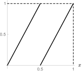
Figure 7.1. $\sigma\left(x\right)=2x$ mod 1

Figure 7.2. Implications and containments. The containments and intersections hold for the sets of measures associated to $\left(X,\mathscr{B},\sigma,R\right)$. Note that in 7.2, $d\lambda=$ Lebesgue measure, $\sigma\left(x\right)=2x$ mod 1; $\lambda\in Fix\left(\sigma\right)\cap\mathscr{L}\left(R\right)$, but $\lambda\notin\mathscr{K}_{1}$. For the various sets referenced in the figure, we refer to 3.11 and 3.4 above.

8. The set $\mathscr{K}_{1}\left(X,\mathscr{B}\right)$

Starting with an endomorphism of a measure space $\left(X,\mathscr{B}\right)$, and a transfer operator $R$ (see, e.g., [Sto13, Rug16, MU15, JR05, Rue04]), we study in the present section an associated family of convex set of measures on $X$ (see 3.11 and 3.13) which yield $R$-regular conditional expectations for the corresponding path-space measure space $\left(\Omega_{X},\mathscr{C},\mathbb{P}\right)$.

Lemma 8.1.

Let $\lambda\in\mathscr{K}_{1}$, then

$$\lambda\circ\sigma^{-1}\in\mathscr{L}\left(R\right)\Longleftrightarrow\lambda\ll\lambda\circ\sigma^{-1}.$$

Proof.

Assume $\lambda\in\mathscr{K}_{1}$, and $\left(\lambda\circ\sigma^{-1}\right)R\ll\lambda\circ\sigma^{-1}$. Since $\left(\lambda\circ\sigma^{-1}\right)R=\lambda$, we get $\lambda\ll\lambda\circ\sigma^{-1}$.

Conversely, suppose $\lambda\ll\lambda\circ\sigma^{-1}$ and $\lambda=\left(\lambda\circ\sigma^{-1}\right)R$. Then we conclude that $\lambda\circ\sigma^{-1}\in\mathscr{L}\left(R\right)$. ∎

Theorem 8.2.

Let $\left(X,\mathscr{B},\sigma,R\right)$ be as usual, assuming $R\mathbbm{1}=\mathbbm{1}$. Suppose $\lambda\in\mathscr{L}\left(R\right)$, and let $W=d\left(\lambda R\right)/d\lambda$.

Then, $\lambda\in\mathscr{K}_{1}$ (so $\lambda\in\mathscr{K}_{1}\cap\mathscr{L}\left(R\right)$) $\Longleftrightarrow$ $W\sim\sigma^{-1}\left(\mathscr{B}\right)$, i.e., $W$ is measurable w.r.t the smaller sigma-algebra $\sigma^{-1}\left(\mathscr{B}\right)$.

Proof.

Set $\nu=\lambda\circ\sigma^{-1}$, and $Q=d\nu/d\lambda$. We show that

$$\lambda\in\mathscr{K}_{1}\Longleftrightarrow\nu R=\lambda\Longleftrightarrow\left(Q\circ\sigma\right)W=1\;\mbox{a.e. }\lambda.$$

(Note that $\lambda\in\mathscr{K}_{1}\Longleftrightarrow\nu R=\lambda$, see (3.19).)

Now compute:

$$\int R\left(f\right)d\nu =\int R\left(f\right)Q\,d\lambda=\int R\left(f\>\left(Q\circ\sigma\right)\right)d\lambda$$

$$=\int f\,\left(Q\circ\sigma\right)d\left(\lambda R\right)=\int f\,\left(Q\circ\sigma\right)W\,d\lambda,$$

and it follows that $\nu R=\lambda\Longleftrightarrow\left(Q\circ\sigma\right)W=1$ a.e. $\lambda$. We need to find a solution $Q$ to

$$\left(Q\circ\sigma\right)\left(x\right)=\begin{dcases}\dfrac{1}{W\left(x\right)}&\mbox{if $W\left(x\right)\neq 0$}\\ 0&\mbox{if $W\left(x\right)=0$}\end{dcases}$$

which is equivalent to $W\sim\sigma^{-1}\left(\mathscr{B}\right)\Longleftrightarrow W^{-1}$ is $\sigma^{-1}\left(\mathscr{B}\right)$-measurable. ∎

8.2 can be restated as follows:

Corollary 8.3.

Suppose $\lambda\in\mathscr{L}\left(R\right)$ with $d\left(\lambda R\right)/d\lambda=W$, then $\lambda\in\mathscr{K}_{1}\left(\cap\mathscr{L}\left(R\right)\right)$ $\Longleftrightarrow$ $\mathbb{E}^{\left(\lambda\right)}\left(W\bigm{|}{}_{\sigma^{-1}\left(\mathscr{B}\right)}\right)=W$, i.e., $W\sim\sigma^{-1}\left(\mathscr{B}\right)$; but the measure $\nu:=\lambda\circ\sigma^{-1}$ may be unbounded.

Remark 8.4.

In general, the solution $\nu$ to $\lambda=\nu R$ may be an unbounded measure.

Meas.	$\mathscr{L}\left(R\right)$	$\mathscr{L}_{1}\left(R\right)$	$Fix\left(\sigma\right)$	$\mathscr{K}_{1}=M_{1}R$	$\sqrt{\lambda}\in\mathscr{H}_{\infty}$	$\underset{{\displaystyle\cap_{i}\mathscr{H}\left(\lambda R^{i}\right)}}{\sqrt{\lambda}\in}$
Defn.	$\lambda R\ll\lambda$	$\lambda R=\lambda$	$\lambda=\lambda\circ\sigma^{-1}$	$\lambda=\nu R$	$\widehat{S}\sqrt{\lambda}=\sqrt{\lambda}$
Ex 7.1	all $\lambda$ s.t. $\lambda\ll dx$ $\lambda_{1}=dx$	(1) $\lambda_{1}=dx$	$\lambda_{1}=dx$	Ex 7.1
$\lambda_{1}=dx$ $\lambda=\lambda R$	$\lambda_{1}=dx$	Ex 7.1
$\lambda_{1}=dx$
Ex 7.2	$\delta_{0}$, $\lambda_{1}=dx$	(2) $\delta_{0}$, singletons	$\delta_{0}$, $\lambda=dx$	$\delta_{0}$
Ex 7.2 $\lambda\notin\mathscr{K}_{1}$	$\delta_{0}$	Ex 7.2
If $\lambda=dx$, then $\cap_{i}\mathscr{H}\left(\lambda R^{i}\right)$
$=0$

Table 8.1. Illustration by Examples. The set of measures itemized in the first two lines of the table refer to the operator $R$ as given in the two examples, Examples 7.1 (line 3), and 7.2 (line 4.) The verification of the respective properties is left to the reader.

9. The universal Hilbert space

Starting with an endomorphism $\sigma$ of a measure space $X$, and a transfer operator $R$, we study in the present section a certain universal Hilbert space which allows an operator realization of the pair $\left(\sigma,R\right)$.

We refer to this as a universal Hilbert space as it involves equivalence classes defined from all possible measures on a fixed measure space, see e.g., [Nel69]. Because of work by [DJ15, DJ06b, Jor04] it is also known that this Hilbert space has certain universality properties.

We shall need the following Hilbert space $\mathscr{H}\left(X\right)$ of equivalence classes of pairs $\left(f,\lambda\right)$, $f\in\mathscr{F}\left(X,\mathscr{B}\right)$, $\lambda\in M\left(X,\mathscr{B}\right)$ (= all Borel measures on $\left(X,\mathscr{B}\right)$).

Definition 9.1.

Two pairs $\left(f,\lambda\right)$ and $\left(g,\mu\right)$ are said to be equivalent, $\left(f,\lambda\right)\sim\left(g,\mu\right)$, iff (Def.) there exists $\xi$ s.t. $\lambda\ll\xi$, $\mu\ll\xi$, and

$$f\sqrt{\frac{d\lambda}{d\xi}}=g\sqrt{\frac{d\mu}{d\xi}}\quad\mbox{a.e. }\xi.$$

The equivalence class of $\left(f,\lambda\right)$ is denoted $f\sqrt{\lambda}$.

Definition 9.2.

Set

$$\bigl{\|}f\sqrt{\lambda}\bigr{\|}_{\mathscr{H}\left(X\right)}^{2} =\int_{X}\left|f\right|^{2}d\lambda,\;\mbox{and}$$

$$\left\langle f_{1}\sqrt{\lambda_{1}},f_{2}\sqrt{\lambda_{2}}\right\rangle_{\mathscr{H}\left(X\right)} =\int_{X}\overline{f_{1}}f_{2}\sqrt{\frac{d\lambda_{1}}{d\mu}}\sqrt{\frac{d\lambda_{2}}{d\mu}}d\mu$$

if $\lambda_{i}\ll\mu$, $i=1,2$.

Lemma 9.3.

Let $\left(X,\mathscr{B},\sigma,R\right)$ be as above, assuming $R\mathbbm{1}=\mathbbm{1}$. Then the mapping

$$\widehat{S}(f\sqrt{\lambda}):=\left(f\circ\sigma\right)\sqrt{\lambda R},\quad\forall f\sqrt{\lambda}\in\mathscr{H}\left(X\right),$$ (9.1)

is well defined and isometric.

Proof.

A direct verification shows that $\widehat{S}$ is well defined. Now we show that $\|\widehat{S}v\|_{\mathscr{H}\left(X\right)}=\left\|v\right\|_{\mathscr{H}\left(X\right)}$, $\forall v\in\mathscr{H}\left(X\right)$. Setting $v=f\sqrt{\lambda}$, we must show that

$$\bigl{\|}f\sqrt{\lambda}\bigr{\|}_{\mathscr{H}\left(X\right)}^{2}=\bigl{\|}\left(f\circ\sigma\right)\sqrt{\lambda R}\bigr{\|}_{\mathscr{H}\left(X\right)}^{2}.$$ (9.2)

Note that

$$\mbox{RHS}_{\left(\ref{eq:h2}\right)} =\int_{X}f^{2}\circ\sigma\,d\left(\lambda R\right)=\int_{X}R\left(f^{2}\circ\sigma\right)d\lambda$$

$$=\int_{X}f^{2}\underset{=\mathbbm{1}}{\underbrace{R\mathbbm{1}}}d\lambda=\int_{X}f^{2}d\lambda=\mbox{LHS}_{\left(\ref{eq:h2}\right)}.$$

∎

Remark 9.4.

9.3 yields the Wold decomposition of $\mathscr{H}\left(X\right)$:

$$\mathscr{H}\left(X\right)=\left(\mbox{Wold shift}\right)\oplus\mathscr{H}_{\infty}$$

where $\mathscr{H}_{\infty}$ denotes the unitary part. See, e.g., [BJ02a, Col09, Jor99, Che80].

Below we outline the operator theoretic details entailed in the analysis in our universal Hilbert space.

Lemma 9.5.

Set

$$\mathscr{H}\left(\mathscr{K}_{1}\right)=\left\{f\sqrt{\lambda}\in\mathscr{H}\left(X\right)\mid\lambda\in\mathscr{K}_{1}\right\}$$ (9.3)

where $\mathscr{K}_{1}=M_{1}R$ (see 3.13). Then $\mathscr{H}\left(\mathscr{K}_{1}\right)\subset\mathscr{H}\left(X\right)$ is a closed subspace.

Definition 9.6.

Let $P_{\mathscr{K}}$ be the orthogonal projection onto $\mathscr{H}\left(\mathscr{K}_{1}\right)$.

Lemma 9.7.

Let $\widehat{S}$ be as in (9.1). Set

$$\widehat{R}\left(g\sqrt{\mu}\right)=R\left(g\right)\sqrt{\mu_{\mathscr{K}}\circ\sigma^{-1}},\quad\sqrt{\mu_{\mathscr{K}}}:=P_{\mathscr{K}}\sqrt{\mu};$$ (9.4)

then $\widehat{S}$, $\widehat{R}$ form a symmetric pair in $\mathscr{H}\left(X\right)$,

$$\left\langle\widehat{S}v,w\right\rangle_{\mathscr{H}\left(X\right)}=\left\langle v,\widehat{R}w\right\rangle_{\mathscr{H}\left(X\right)},\quad\forall v,w\in\mathscr{H}\left(X\right).$$ (9.5)

That is,

$$\widehat{R}=\widehat{S}^{*}.$$ (9.6)

Proof.

We note that (9.5) $\Longleftrightarrow$

$$\left\langle f\circ\sigma\sqrt{\lambda R},g\sqrt{\mu}\right\rangle_{\mathscr{H}\left(X\right)}=\left\langle f\sqrt{\lambda},R\left(g\right)\sqrt{\mu_{\mathscr{K}}\circ\sigma^{-1}}\right\rangle_{\mathscr{H}\left(X\right)},$$ (9.7)

$\forall f\sqrt{\lambda},g\sqrt{\mu}\in\mathscr{H}\left(X\right)$.

To verify (9.7):

$$\mbox{RHS}_{\left(\ref{eq:h6}\right)}=\int_{X}fR\left(g\right)\sqrt{\frac{d\lambda}{d\xi}\frac{d\mu_{\mathscr{K}}\circ\sigma^{-1}}{d\xi}}d\xi$$

and

$$\mbox{LHS}_{\left(\ref{eq:h6}\right)} =\int_{X}\left(f\circ\sigma\right)g\sqrt{\frac{d\left(\lambda R\right)}{d\left(\xi R\right)}\cdot\frac{d\mu}{d\left(\xi R\right)}}d\left(\xi R\right)$$

$$=\int_{X}\left(f\circ\sigma\right)g\sqrt{\left(\frac{d\lambda}{d\xi}\right)\circ\sigma\cdot\left(\frac{d\mu_{\mathscr{K}}\circ\sigma^{-1}}{d\xi}\right)\circ\sigma}\,d\left(\xi R\right)$$

$$=\int_{X}fR\left(g\right)\sqrt{\left(\frac{d\lambda}{d\xi}\right)\frac{d\mu_{\mathscr{K}}\circ\sigma^{-1}}{d\xi}}d\xi=\mbox{RHS}_{\left(\ref{eq:h6}\right)},$$

where we used the following substitution rules (see 3.16)

$$\frac{d\left(\lambda R\right)}{d\left(\xi R\right)} =\frac{d\lambda}{d\xi}\circ\sigma$$

$$\frac{d\mu}{d\left(\xi R\right)} =\left(\frac{d\mu_{\mathscr{K}}\circ\sigma^{-1}}{d\xi}\right)\circ\sigma$$

for the respective Radon-Nikodym derivatives.

Note that we also used that

$$\left[\begin{array}[]{c}\lambda\ll\xi\\ \mu_{\mathscr{K}}\circ\sigma^{-1}\ll\xi\end{array}\right]\Longrightarrow\left[\begin{array}[]{c}\lambda R\ll\xi R\\ \mu\ll\xi R\end{array}\right].$$

∎

Corollary 9.8.

Given $\left(X,\mathscr{B},\sigma,R\right)$, $R\mathbbm{1}=\mathbbm{1}$, as introduced above. Let $\widehat{S}$, $\widehat{R}=\widehat{S}^{*}$ be the canonical operators in $\mathscr{H}\left(X\right)$, then

1. $\widehat{R}\widehat{S}=\widehat{S}^{*}\widehat{S}=I_{\mathscr{H}\left(X\right)}$ ;

2. $\widehat{S}\widehat{R}=\widehat{S}\widehat{S}^{*}=\widehat{E}_{1}$ = the projection onto $\widehat{S}\mathscr{H}\left(X\right)$; and

3. $\widehat{E}_{1}\bigl{(}f\sqrt{\lambda}\bigr{)}=R\left(f\right)\circ\sigma\sqrt{\lambda_{\mathscr{K}}}$, where $\sqrt{\lambda_{\mathscr{K}}}=P_{\mathscr{K}}\sqrt{\lambda}$.

Proof.

We already proved (1)-(2); recall that

$$f\sqrt{\lambda}\xrightarrow{\;\widehat{S}\;}f\circ\sigma\sqrt{\lambda R}\xrightarrow{\;\widehat{R}\;}R\left(f\circ\sigma\right)\sqrt{\lambda R\circ\sigma^{-1}}=f\sqrt{\lambda}.$$

Proof of (3).

$$\widehat{E}_{1}\left(f\sqrt{\lambda}\right) =\widehat{S}\widehat{R}f\sqrt{\lambda}=\widehat{S}\left(R\left(f\right)\sqrt{\lambda_{\mathscr{K}}\circ\sigma^{-1}}\right)$$

$$=R\left(f\right)\circ\sigma\sqrt{\lambda_{\mathscr{K}}\circ\sigma^{-1}R}=R\left(f\right)\circ\sigma\sqrt{\lambda_{\mathscr{K}}}.$$

In the last step we used that $\lambda_{\mathscr{K}}\in\mathscr{K}_{1}$ s.t. $\left(\lambda_{\mathscr{K}}\circ\sigma^{-1}\right)R=\lambda_{\mathscr{K}}$, and the conditional expectation on $\sigma^{-1}\left(\mathscr{B}\right)$, i.e., $\mathbb{E}^{\left(\lambda_{\mathscr{K}}\right)}\left(f\mid\sigma^{-1}\left(\mathscr{B}\right)\right)$; see 5.1. ∎

Question 9.9.

In 7.2 with $\lambda=dx=$Lebesgue, what is $\lambda_{\mathscr{K}}$, i.e., $\sqrt{\lambda_{\mathscr{K}}}=\mbox{Proj}_{\mathscr{K}_{1}}(\sqrt{\lambda})$? See 9.11 below.

Lemma 9.10.

We can establish the increasing sets

$$\mathscr{L}\left(R\right)\subseteq\mathscr{L}\left(R^{2}\right)\subseteq\mathscr{L}\left(R^{3}\right)\subseteq\cdots$$ (9.8)

as follows:

$$\mathscr{L}\left(R\right)\xhookrightarrow{\quad\widehat{R}\quad}\mathscr{L}\left(R^{2}\right)\xhookrightarrow{\quad\widehat{R}\quad}\mathscr{L}\left(R^{4}\right)\xhookrightarrow{\quad\widehat{R}\quad}\cdots$$ (9.9)

Proof.

For (9.9), since $\lambda\in\mathscr{L}\left(R\right)$, $\lambda R\ll\lambda$, and $\widehat{R}\sqrt{\lambda}=\sqrt{\lambda_{\mathscr{K}}\circ\sigma^{-1}}$, so $\widehat{R}\mathscr{L}\left(R\right)\subset\mathscr{L}\left(R^{2}\right)$ as

$$\left(\lambda_{\mathscr{K}}\circ\sigma^{-1}\right)R^{2}=\underset{\lambda_{\mathscr{K}}}{\underbrace{\left(\lambda_{\mathscr{K}}\circ\sigma^{-1}\right)R}}R=\lambda_{\mathscr{K}}R\ll\lambda.$$

(Note the containment in (9.8) refers to measure classes in $\mathscr{H}\left(X\right)$. See also 3.17.) ∎

Remark 9.11.

Let $\left(X,\mathscr{B},\sigma,R\right)$, $R\mathbbm{1}=\mathbbm{1}$ be as usual, and let $\widehat{S}$, and $\widehat{R}=\widehat{S}^{*}$ be the universal operators; see (9.1) and (9.4).

If, in addition, $\lambda\in\mathscr{L}\left(R\right)$ with $d\left(\lambda R\right)/d\lambda=W$, then we also have

$$\widehat{R}\left(f\sqrt{\lambda}\right)=R\left(\frac{f}{\sqrt{W}}\right)\sqrt{\lambda}.$$ (9.10)

Proof.

Eq (9.10) is verified as follows:

$$\left\langle f\circ\sigma\sqrt{\lambda R},g\sqrt{\lambda}\right\rangle_{\mathscr{H}\left(X\right)} =\int_{X}\left(f\circ\sigma\right)g\sqrt{W}d\lambda=\int_{X}\frac{\left(f\circ\sigma\right)g}{\sqrt{W}}d\left(\lambda R\right)$$

$$=\int_{X}fR\left(\frac{g}{\sqrt{W}}\right)d\lambda=\left\langle f\sqrt{\lambda},R\left(\frac{g}{\sqrt{W}}\sqrt{\lambda}\right)\right\rangle_{\mathscr{H}\left(X\right)}.$$

∎

Corollary 9.12.

Suppose $\lambda\in\mathscr{L}\left(R\right)$, $d\left(\lambda R\right)/d\lambda=W$, then

$$\lambda\ll\lambda_{\mathscr{K}}\circ\sigma^{-1},\;\mbox{and}\quad\frac{d\lambda}{d\left(\lambda_{\mathscr{K}}\circ\sigma^{-1}\right)}=W\circ\sigma^{-1}.$$ (9.11)

Proof.

From 9.11 we have

$$\left(R\left(f\right),\lambda_{\mathscr{K}}\circ\sigma^{-1}\right)\sim\left(R\left(\frac{f}{\sqrt{W}}\right),\lambda\right)$$ (9.12)

and since $\lambda R\ll\lambda$, we get $\lambda\ll\lambda_{\mathscr{K}}\circ\sigma^{-1}$. So (9.12) $\Longrightarrow$

$$R\left(f\right)=R\left(\frac{f}{\sqrt{W}}\right)\sqrt{\frac{d\lambda}{d\left(\lambda_{\mathscr{K}}\circ\sigma^{-1}\right)}}=R\left(\left(\frac{f}{\sqrt{W}}\right)\sqrt{W}\right),$$

and (9.11) follows. ∎

Corollary 9.13.

Suppose $\lambda\in\mathscr{L}\left(R\right)$, $d\left(\lambda R\right)/d\lambda=W$, then

$$P_{\mathscr{K}}\sqrt{\lambda}=\frac{1}{\sqrt{W}}\sqrt{\lambda R}.$$

Proof.

Follows from 9.11. ∎

Lemma 9.14.

Let $\left(X,\mathscr{B},\sigma,R\right)$ be as above, $R\mathbbm{1}=\mathbbm{1}$. Suppose $\mu R\ll\mu$, $\frac{d\mu R}{d\mu}=W$. Then

1. $S:f\longrightarrow f\circ\sigma\sqrt{W}$ is isometric in $L^{2}\left(\mu\right)$; and

2. we have $R^{*}:f\longrightarrow\left(f\circ\sigma\right)W$ in $L^{2}\left(\mu\right)$.

Proof.

We check that

(1)

$$\int\left(\left(f\circ\sigma\right)\sqrt{W}\right)^{2}d\mu=\int f^{2}\circ\sigma Wd\mu=\int R\left(f^{2}\circ\sigma\right)d\mu=\int f^{2}d\mu;$$

(2)

$$\int\left(f\circ\sigma\right)Wgd\mu=\int\left(f\circ\sigma\right)g\,d\mu R=\int R\left(\left(f\circ\sigma\right)g\right)d\mu=\int fR\left(g\right)d\mu.$$

∎

10. Ergodic limits

We now turn to a number of ergodic theoretic results that are feasible in the general setting of pairs $\left(\sigma,R\right)$. See, e.g., [Yos80], and also Definitions 3.11, 9.1 and Lemmas 9.3, 9.7.

Theorem 10.1.

Given $\left(X,\mathscr{B},\sigma,R\right)$, $R\mathbbm{1}=\mathbbm{1}$, as usual; then the following two conditions are equivalent:

$$\bigcap_{i}\mathscr{L}\left(\lambda R^{i}\right)\neq 0$$

$$\Updownarrow$$

$$\lim_{N\rightarrow\infty}\underset{=:A_{N}}{\underbrace{\frac{1}{N}\sum_{k=1}^{N}\prod_{j=0}^{k-1}\sqrt{W\circ\sigma^{j}}}}\neq 0\;\mbox{in }L^{2}\left(\lambda\right),\;\mbox{i.e.,}$$ (10.1)

$$\lim_{N\rightarrow\infty}\frac{1}{N}\sum_{k=1}^{n}\sqrt{W\left(W\circ\sigma\right)\cdots\left(W\circ\sigma^{k-1}\right)}=W_{\infty}\in L^{2}\left(\lambda\right),\;\mbox{where}$$

$$W_{\infty}\neq 0,\;\mbox{and }\int W_{\infty}d\lambda\leq 1.$$

Remark 10.2.

Existence of the limit in (10.1) is automatic.

Proof.

Return to $\mathscr{H}\left(X\right)$, $\widehat{S}$ and $\widehat{R}$, and suppose

$$\mu R\ll\mu;$$ (10.2)

so

(10.3)

where we used:

$$\widehat{S}\left(f\sqrt{\lambda}\right):=\left(f\circ\sigma\right)\sqrt{\lambda R},\quad\forall f\sqrt{\lambda}\in\mathscr{H}\left(X\right).$$ (10.4)

We note that

$$\frac{1}{N}\sum_{k=1}^{N}\widehat{S}^{k}\longrightarrow\widehat{E}_{1}$$

where $\widehat{E}_{1}$ is the projection in $\mathscr{H}\left(X\right)$ onto $\left\{w_{1}\in\mathscr{H}\left(X\right)\mid\widehat{S}w_{1}=w_{1}\right\}$. This is a version of von Neumann’s ergodic theorem; see e.g., [Yos80]. Thus

$$\lim_{N\rightarrow\infty}\left\|\widehat{A}_{N}\sqrt{\mu}-\widehat{E}_{1}\sqrt{\mu}\right\|_{\mathscr{H}\left(X\right)}=0.$$ (10.5)

∎

Theorem 10.3.

Let $\left(X,\mathscr{B},\sigma,R\right)$, $R\mathbbm{1}=\mathbbm{1}$, be as above. Let $\lambda\in\mathscr{L}\left(R\right)$, $\frac{d\lambda R}{d\lambda}=W$, and set

$$A_{N}=\frac{1}{N}\sum_{k=1}^{N}\prod_{j=0}^{k-1}\sqrt{W\circ\sigma^{j}};$$ (10.6)

then $\exists W_{\infty}\in L^{2}\left(\lambda\right)$ s.t.

$$A_{N}\xrightarrow[\;N\rightarrow\infty\;]{}W_{\infty}\;\mbox{pointwise }\lambda\mbox{-a.e.}$$ (10.7)

Proof.

We saw that the sequence in (10.6) corresponds to the measure ergodic limit $\lim_{N}\frac{1}{N}\sum_{k=1}^{N}\widehat{S}$ as an operator limit in $\mathscr{H}\left(X\right)$ since $\widehat{S}$ is isometric. Hence (10.6) has a subsequence which converges $\lambda$ a.e. But since

$$\frac{1}{N+1}\prod_{k=0}^{N}\sqrt{W\circ\sigma^{k}}\longrightarrow 0,\;\mbox{and}$$

$$A_{N+1}=\frac{N}{N+1}A_{N}+\frac{1}{N+1}\prod_{k=0}^{N}\sqrt{W\circ\sigma^{k}}$$ (10.8)

we conclude that $\left\{A_{N}\right\}_{N\in\mathbb{Z}_{+}}$ converges itself, $\lambda$-a.e., as $N\longrightarrow\infty$.

Indeed, we assume $\lambda\in\mathscr{L}\left(R\right)$; set $W=\frac{d\lambda R}{d\lambda}$,

$$\left\|\frac{1}{N}\sum_{k=1}^{N}\widehat{S}^{k}\sqrt{\lambda}-W_{\infty}\sqrt{\lambda}\right\|_{\mathscr{H}\left(X\right)}\xrightarrow[\;N\rightarrow\infty\;]{}0$$ (10.9)

$$\Updownarrow$$

$$\left\|\frac{1}{N}\sum_{k=1}^{N}\prod_{j=0}^{k-1}\sqrt{W\circ\sigma^{j}}-W_{\infty}\right\|_{L^{2}\left(\lambda\right)}\xrightarrow[\;N\rightarrow\infty\;]{}0$$ (10.10)

and (10.8) $\Leftrightarrow$ (10.9) $\Leftrightarrow$ (10.10). But by the von Neumann-Yosida ergodic theorem [Yos80], the limit in (10.9) automatically exists. Hence $W_{\infty}\in L^{2}\left(\lambda\right)$, the limit function may be zero; this holds in 7.2, $\lambda=dx=$ Lebesgue measure, i.e.,

$$\frac{1}{N+1}\prod_{j=0}^{N}\sqrt{W\circ\sigma^{j}}\xrightarrow[\;N\rightarrow\infty\;]{}0.$$ (10.11)

Now it follows from the general ergodic theorem; the von Neumann-Yosida theorem in the Hilbert space $\mathscr{H}\left(X\right)$, or in $\mathscr{H}\left(\mu\right)$, that the limit exists, where:

$$A_{N}\left(\sqrt{\mu}\right)\xrightarrow[\;N\rightarrow\infty\;]{}\widehat{E}_{1}\left(\sqrt{\mu}\right)\;\mbox{exists},$$ (10.12)

but $\sqrt{\mu_{\infty}}$ may be zero (see 7.2).

We shall establish that the limit function

$$\lim_{N\rightarrow\infty}\frac{1}{N}\sum_{k=1}^{N}\prod_{j=0}^{k-1}\sqrt{W\circ\sigma^{j}}=W_{\infty}$$ (10.13)

is a non-zero function in $L^{2}\left(X,\mu\right)$.

Suppose $0\leq W\leq 1$ pointwise, then we get the formula

$$A_{N}=\frac{1}{N}\sum_{k=1}^{N}\prod_{j=0}^{k-1}\sqrt{W\circ\sigma^{j}}$$

and monotone decreasing as $N\longrightarrow\infty$:

$$A_{N}-A_{N+1}$$

$$= \frac{1}{N}\left[\sqrt{W}+\sqrt{W}\sqrt{W\circ\sigma}+\cdots+\sqrt{W}\sqrt{W\circ\sigma}\cdots\sqrt{W\circ\sigma^{N-1}}\right]$$

$$-\frac{1}{N+1}\left[\sqrt{W}+\sqrt{W}\sqrt{W\circ\sigma}+\cdots+\sqrt{W}\sqrt{W\circ\sigma}\cdots\sqrt{W\circ\sigma^{N}}\right]$$

$$= \frac{1}{N+1}\left[\sqrt{W}+\sqrt{W}\sqrt{W\circ\sigma}+\cdots+\sqrt{W}\cdots\sqrt{W\circ\sigma^{N-1}}\right]$$

$$-\frac{1}{N+1}\sqrt{W}\cdots\sqrt{W\circ\sigma^{N}}\geq 0.$$

(7.2 illustrates $A_{N}\longrightarrow 0$ is possible, since in this case $\bigcap_{i}\mathscr{H}\left(\lambda R^{i}\right)=0$, where $\lambda=dx=$ Lebesgue measure.)

Since $\widehat{S}$ is an isometry in $\mathscr{H}\left(X\right)$, we apply Wold’s theorem [BJ02a, Col09, Jor99, Che80] to get existence of the limit in (10.11), so $\exists\mu_{\infty}\in M_{+}$, $\sqrt{\mu_{\infty}}\in\mathscr{H}\left(X\right)$ s.t.

$$\lim_{N\rightarrow\infty}\left\|\sqrt{\mu_{\infty}}-\frac{1}{N}\left(\sum_{k=1}^{N}\widehat{S}^{k}\right)\left(\sqrt{\lambda}\right)\right\|_{\mathscr{H}\left(X\right)}=0,$$

and $\mu_{\infty}=\mu_{\infty}R$. (Note. $\mu_{\infty}\ll\lambda$, but $\mu_{\infty}=0$ is possible. This is precisely what happens in 7.2.)

Pass to $\widehat{S}$, $\mathscr{H}\left(X\right)$, where $\widehat{S}\left(f\sqrt{\mu}\right)=\left(f\circ\sigma\right)\sqrt{\mu R}$, $\forall f\sqrt{\mu}\in\mathscr{H}\left(X\right)$, then $\widehat{S}$ is isometric in $\mathscr{H}\left(X\right)$ (see 9.3), and if $\lambda\in\mathscr{L}\left(R\right)$ then $\widehat{S}$ restricts to an isometry in $\mathscr{H}\left(\lambda\right)\simeq L^{2}\left(\lambda\right)$ (unitary), and

$$\widehat{S}^{k}\sqrt{\lambda}=\sqrt{\lambda R^{k}}=\sqrt{W\left(W\circ\sigma\right)\cdots W\circ\sigma^{k-1}}\sqrt{\lambda},$$

and by the general theorem (von Neumann and Yosida), $\frac{1}{N}\sum_{k=1}^{N}\widehat{S}^{k}\sqrt{\lambda}$ exists in $\mathscr{H}\left(\lambda\right)$. ∎

Lemma 10.4.

Let $\left(X,\mathscr{B},\sigma,R\right)$, $R\mathbbm{1}=\mathbbm{1}$, be as above. Suppose $\lambda R\ll\lambda$, $W=\frac{d\lambda R}{d\lambda}$, and let $\mu_{\alpha}$ be a measure on $\left(X,\mathscr{B}\right)$ s.t.

$$\lim_{N\rightarrow\infty}\left\|\sqrt{\mu_{\alpha}}-\frac{1}{N}\sum_{k=1}^{N}\widehat{S}^{k}\sqrt{\lambda}\right\|_{\mathscr{H}\left(X\right)}=0.$$ (10.14)

Recall $\widehat{S}^{k}\sqrt{\lambda}=\prod_{j=0}^{k-1}\sqrt{W\circ\sigma^{j}}\sqrt{\lambda}$, and (10.14) is equivalent to

$$\int_{X}\left|W_{\infty}-A_{N}\right|^{2}d\lambda\xrightarrow[\;N\rightarrow\infty\;]{}0.$$ (10.15)

Then, $\mu_{\infty}R=\mu_{\alpha}$ and $\mu_{\infty}\ll\lambda$, where $d\mu_{\infty}=W_{\infty}d\lambda$, $W_{\infty}\in L^{2}\left(\lambda\right)$, and $\sqrt{\mu_{\infty}}\in\mathscr{H}\left(\lambda\right)$. However, $\mu_{\infty}=0$ is possible.

Remark 10.5.

7.2 shows that $\mu_{\infty}=0$ is possible.

We do have a general condition:

Proposition 10.6.

Assume $\lambda R\ll\lambda$, $W=\frac{d\lambda R}{d\lambda}$, then

$$\frac{1}{N}\sum_{k=1}^{N}\widehat{S}^{k}\sqrt{\lambda}\xrightarrow[\;N\rightarrow\infty\;]{}\sqrt{W_{\infty}\lambda}$$ (10.16)

$$\Updownarrow$$

$$\underset{=:A_{N}}{\underbrace{\frac{1}{N}\sum_{k=1}^{N}\prod_{j=0}^{k-1}\sqrt{W\circ\sigma^{j}}\sqrt{\lambda}}}\quad\mbox{has a limit in }L^{2}\left(\lambda\right).$$ (10.17)

Question 10.7.

Is it still possible that $\exists\mu_{\infty}\in M_{1}$ s.t.

$$\lim_{N\rightarrow\infty}\frac{1}{N}\sum_{k=1}^{N}\widehat{S}^{k}\sqrt{\lambda}=\sqrt{\mu_{\infty}},$$ (10.18)

and $\mu_{\infty}R=\mu_{\infty}$, and $\mu_{\infty}\ll\lambda$?

Proof of 10.6.

Note that $\lambda R\ll\lambda$ $\Longrightarrow$ $\widehat{S}$ in $\mathscr{H}\left(X\right)$. Indeed, $\widehat{S}\mathscr{H}\left(\lambda\right)\subset\mathscr{H}\left(\lambda\right)$, which is closed in $\mathscr{H}\left(X\right)$. To see this, we check that

$$\widehat{S}f\sqrt{\lambda}=\left(f\circ\sigma\right)\sqrt{\lambda R}=\left(f\circ\sigma\right)\sqrt{W}\sqrt{\lambda}\in\mathscr{H}\left(\lambda\right)$$

and

$$\left\|\left(f\circ\sigma\right)\sqrt{W}\sqrt{\lambda}\right\|_{\mathscr{H}\left(\lambda\right)}^{2}=\int\left(f^{2}\circ\sigma\right)\underset{\lambda R}{\underbrace{Wd\lambda}}=\int f^{2}d\lambda=\left\|f\right\|_{L^{2}\left(\lambda\right)}^{2},$$

which implies that

$$A_{N}\sqrt{\lambda}=\frac{1}{N}\sum_{k=1}^{N}\widehat{S}^{k}\sqrt{\lambda}\in\mathscr{H}\left(\lambda\right),$$

and $\mathscr{H}\left(\lambda\right)$ is closed in $\mathscr{H}\left(X\right)$. Therefore, $A_{N}\sqrt{\lambda}\longrightarrow\widehat{E}_{1}\sqrt{\lambda}$, $\widehat{E}_{1}\sqrt{\lambda}=\sqrt{d\mu_{\infty}}$, and $\mu_{\infty}R=\mu_{\infty}$. ∎

11. $\mathscr{L}_{1}\left(R\right)$ as a subspace of $\mathscr{L}\left(R\right)$

In the present section we study Radon-Nikodym properties of the path-space measures from Sections 5 and 10.

Lemma 11.1.

Suppose $\lambda_{1}R=\lambda_{1}$, and $\mu\ll\lambda_{1}$; then $\mu\in\mathscr{L}\left(R\right)$, i.e., we have $\mu R\ll\mu$.

Proof.

Let $\frac{d\mu}{d\lambda_{1}}=W$, $W\in L^{1}\left(\lambda_{1}\right)$ and set

$$Q\left(x\right)=\begin{dcases}\frac{W\left(\sigma\left(x\right)\right)}{W\left(x\right)}&\mbox{if }W\left(x\right)>0\\ 0&\mbox{if }W\left(x\right)=0\end{dcases};$$

then

$$\int f\,d\left(\mu R\right) =\int R\left(f\right)d\mu=\int_{\left\{x:W\left(x\right)>0\right\}}R\left(f\right)Wd\lambda_{1}$$

$$=\int R\left(f\left(W\circ\sigma\right)\right)d\lambda_{1}$$

$$=\int f\frac{W\circ\sigma}{W}Wd\lambda_{1}\;(\mbox{since }\lambda_{1}R=\lambda_{1})$$

$$=\int f\,Q\,d\mu.$$

Thus, $\mu R\ll\mu$ and $\frac{d\mu R}{d\mu}=Q$. ∎

Remark 11.2.

There are several interesting questions as to whether there is an inverse implication. In “most” cases of $\mu$ satisfying $\mu R\ll\mu$, then $\exists\mu_{\infty}\in M_{+}$ s.t. $\mu_{\infty}R=\mu_{\infty}$, and $\mu_{\infty}\ll\mu$. (See 7.2.)

Lemma 11.3.

Let $\left(X,\mathscr{B},\sigma,R\right)$, $R\mathbbm{1}=\mathbbm{1}$, be as usual. Suppose $\lambda\in M_{1}$, $\mu\in\mathscr{L}\left(R\right)$, and $\frac{d\lambda R}{d\lambda}=W$; then

$$1= \int Wd\lambda=\int\left(W\circ\sigma\right)Wd\lambda=\cdots$$ (11.1)

$$\cdots=\int\left(W\circ\sigma^{n}\right)\cdots\left(W\circ\sigma\right)Wd\lambda=1.$$

More over, the following GENERAL estimates hold:

$$\int\sqrt{W}d\lambda \leq 1$$

$$\int\sqrt{\left(W\circ\sigma\right)W}d\lambda \leq 1$$ (11.2)

$$\vdots$$

$$\int\sqrt{\left(W\circ\sigma^{n}\right)\cdots\left(W\circ\sigma\right)W}d\lambda \leq 1$$

Proof.

We note that $\widehat{S}$ is isometric, where

$$\widehat{S}\bigl{(}\sqrt{\lambda}\bigr{)} =\sqrt{\lambda R}=\sqrt{W}\sqrt{\lambda}$$

$$\widehat{S}^{2}\bigl{(}\sqrt{\lambda}\bigr{)} =\sqrt{\left(W\circ\sigma\right)W}\sqrt{\lambda}.$$

So $1=\bigl{\|}\sqrt{d\lambda}^{2}\bigr{\|}=\bigl{\|}\widehat{S}\sqrt{\lambda}\bigr{\|}^{2}=\bigl{\|}\widehat{S}^{2}\sqrt{\lambda}\bigr{\|}^{2}=\cdots=1$, i.e., (11.1) holds. ∎

Remark 11.4.

The conditions in (11.2) are satisfied in 7.2, where $\lambda=dx=$ Lebesgue measure,

$$W\left(x\right)=2\cos^{2}\left(\pi x\right)=1+\cos\left(2\pi x\right),$$

and $\int W\left(x\right)dx=1$. So

$$\frac{1}{N+1}\sqrt{\left(W\circ\sigma^{n}\right)\cdots\left(W\circ\sigma\right)W}\xrightarrow[\;N\rightarrow\infty\;]{}0\quad\mbox{in $L^{2}\left(\lambda\right)=L^{2}\left(dx\right)$.}$$

12. Multiresolutions from endomorphisms and solenoids

We now return to a more detailed analysis of the multi-scale resolutions introduced in 5 above.

General setting: Let $\left(X,\mathscr{B},\sigma,R\right)$, $R\mathbbm{1}=\mathbbm{1}$, be as usual.

Multiresolution $\longleftrightarrow$ wavelets (5.2), with levels of resolution given by

$$\mathscr{B}\supseteq\sigma^{-1}\left(\mathscr{B}\right)\supseteq\sigma^{-2}\left(\mathscr{B}\right)\supseteq\cdots\supseteq\mathscr{B}_{\infty},$$ (12.1)

$$\sigma^{-i}\left(\mathscr{B}\right)=\underset{\text{details in between}}{\underbrace{\left[\sigma^{-i}\left(\mathscr{B}\right)\backslash\sigma^{-\left(i+1\right)}\left(\mathscr{B}\right)\right]}}\cup\sigma^{-\left(i+1\right)}\left(\mathscr{B}\right);$$ (12.2)

i.e., $\mathscr{B}$ is space of initial resolution, $\sigma^{-1}\left(\mathscr{B}\right)$ contains less information; see, e.g., [BJ02b, BJ02a, BJMP05, AJLV16, BRC16, KFB16, SG16]

If $\mu\in\mathscr{L}\left(R\right)\cap\mathscr{K}_{1}$, then we have the following resolution decomposition:

$$\cdots\subset L_{\mathscr{H}}^{2}\left(\mu R^{2}\right)\subset L_{\mathscr{H}}^{2}\left(\mu R\right)\subset L_{\mathscr{H}}^{2}\left(\mu\right)$$ (12.3)

Note that $\widehat{S}\widehat{S}^{*}=\widehat{E}_{1}=$ projection onto $\widehat{S}\mathscr{H}\left(X\right)$, but if restrict to $\mathscr{H}\left(\mu\right)$, it is the projection onto $\mathscr{H}\left(\mu R\right)$.

Recall that, by 9.8, we have $\mathbb{E}^{\left(\mu\right)}\left(f\mid\sigma^{-1}\left(\mathscr{B}\right)\right)=\widehat{S}\widehat{S}^{*}\big{|}_{\mathscr{H}\left(\mu\right)}\left(f\right)$, i.e.,

$$\widehat{S}\widehat{S}^{*}\left(f\sqrt{\mu}\right)=\mathbb{E}^{\left(\mu\right)}\left(f\mid\sigma^{-1}\left(\mathscr{B}\right)\right)\sqrt{\mu}$$ (12.4)

so that

$$\underset{\widehat{E}_{i}}{\underbrace{\widehat{S}^{i}\widehat{S}^{*i}}}\left(f\sqrt{\mu}\right)=\mathbb{E}^{\left(\mu\right)}\left(f\mid\sigma^{-i}\left(\mathscr{B}\right)\right)\sqrt{\mu},\quad i=1,2,3\cdots.$$

Theorem 12.1.

Wavelet decomposition for $h\in\mathscr{H}\left(\mu\right)$:

$$h= k_{0}+\left(k_{1}\circ\sigma\right)\sqrt{W}+\left(k_{2}\circ\sigma^{2}\right)\sqrt{W\left(W\circ\sigma\right)}+\cdots$$

$$\cdots+\left(k_{n}\circ\sigma^{n}\right)\sqrt{W\left(W\circ\sigma\right)\left(W\circ\sigma^{2}\right)\cdots\left(W\circ\sigma^{n-1}\right)}+\cdots+h_{\infty}$$ (12.5)

as a decomposition in $\mathscr{H}\left(\mu\right)\sim L^{2}\left(\mu\right)$.

Proof.

We use Wold on $\widehat{S}\big{|}_{\mathscr{H}\left(\mu\right)}$ as an isometry. (See [BJ02a, Col09, Jor99, Che80].) Note, if $\mu R\ll\mu$, then $\widehat{S}\mathscr{H}\left(\mu\right)\subset\mathscr{H}\left(\mu\right)$ so that it is isometric in $\mathscr{H}\left(\mu\right)\sim L^{2}\left(\mu\right)$.

If $\lambda R=1$ then $Sf=f\circ\sigma$ is isometric in $L^{2}\left(\lambda\right)$, and $S^{*}=R$ relative to the $L^{2}\left(\lambda\right)$-inner product, so $RS\Big{|}_{L^{2}\left(\lambda\right)}=I$, $SR=SS^{*}=E_{1}=$ the projection onto $SL^{2}\left(\lambda\right)$, and $E_{1}L^{2}\left(\lambda\right)=SL^{2}\left(\lambda\right)$, $I-E_{1}=$ the projection onto

$$\left(SL^{2}\left(\lambda\right)\right)^{\perp}=\ker S^{*}=\ker R=\left\{f\in L^{2}\left(\lambda\right)\mid Rf=0\right\}.$$

The orthogonal expansion for $f\in L^{2}\left(\lambda\right)$ is as follows:

$$f=h_{0}+Sh_{1}+S^{2}h_{2}+\cdots+S^{n}h_{n}+\cdots+h_{\infty},$$

and by Parseval’s identity:

$$\left\|f\right\|_{L^{2}\left(\lambda\right)}^{2}=\sum_{n=0}^{\infty}\left\|h_{n}\right\|_{L^{2}\left(\lambda\right)}^{2}+\left\|h_{\infty}\right\|_{L^{2}\left(\lambda\right)}^{2}.$$

Note in $L^{2}\left(\lambda\right)$,

$$SRf =\mathbb{E}^{\left(\lambda\right)}\left(f\mid\sigma^{-1}\left(\mathscr{B}\right)\right),$$

$$S^{n}R^{n}f =\mathbb{E}^{\left(\lambda\right)}\left(f\mid\sigma^{-n}\left(\mathscr{B}\right)\right),$$

$$E_{\infty}f =\mathbb{E}^{\left(\lambda\right)}\left(f\mid\mathscr{B}_{\infty}\right),$$

where $\mathscr{B}_{\infty}=\cap_{n=1}^{\infty}\sigma^{-n}\left(\mathscr{B}\right)$. ∎

13. Application to Examples 7.1 & 7.2

We now return to a more detailed analysis of the two examples from 7 above.

Example 13.1 (See Ex 7.1).

Consider $X=\mathbb{R}/\mathbb{Z}\simeq[0,1)$, $\lambda=dx=$ Lebesgue measure on $\left[0,1\right]$.

Set $\sigma\left(x\right)=2x$ mod 1, $Sf\left(x\right)=f\left(2x\right)$ in $L^{2}\left(\left[0,1\right],\lambda\right)$. Then $S^{*}=R$,

$$\left(Rf\right)\left(x\right)=\frac{1}{2}\Bigl{(}f\Bigl{(}\frac{x}{2}\Bigr{)}+f\Bigl{(}\frac{x+1}{2}\Bigr{)}\Bigr{)},$$ (13.1)

and $S^{*}k=0$ $\Longleftrightarrow$ $\exists h$ s.t. $k\left(x\right)=e_{1}\left(x\right)h\left(2x\right)=e_{1}\left(x\right)h\left(\sigma\left(x\right)\right)$, where $h\in L^{2}\left(\lambda\right)$, and $e_{1}\left(x\right)=e^{i2\pi x}$.

Proposition 13.2.

For all $f\in L^{2}\left(\lambda\right)$, there a unique orthogonal expansion:

$$f\left(x\right)= e_{1}\left(x\right)h_{0}\left(2x\right)+e_{1}\left(3x\right)h_{1}\left(2^{2}x\right)+\cdots$$

$$\cdots+e_{1}\left(\left(2^{n}-1\right)x\right)h_{n}\left(2^{n}x\right)+\cdots+\mbox{const};$$

and

$$\left\|f\right\|_{\lambda}^{2}=\sum_{n=0}^{\infty}\left\|h_{n}\right\|_{\lambda}^{2}+\left\|f_{\infty}\right\|_{\lambda}^{2},\quad f_{\infty}=\mbox{const.}$$

In the general case we get, for all $h\in\mathscr{H}\left(\mu\right)$:

$$h=k_{0}\sqrt{\mu}+\left(k_{1}\circ\sigma\right)\sqrt{\mu R}+\left(k_{2}\circ\sigma^{2}\right)\sqrt{\mu R^{2}}+\cdots+h_{\infty},$$

where $h_{\infty}\in\cap_{i}\widehat{S}^{i}\mathscr{H}\left(\mu\right)$. See 13.1, and also Sections 5.1, 5.3.

Figure 13.1. Multiresolution expansion.

Example 13.3 (Ex 13.1 continued).

Let $R$ be as in (13.1). In the real case, we have two solutions to $Rf=0$:

$$f_{c}\left(x\right)=\cos\left(2\pi x\right),\quad f_{s}\left(x\right)=\sin\left(2\pi x\right).$$

Allowing complex functions we have

$$e_{\pm}\left(x\right)=e^{\pm i2\pi x}.$$

We also check directly that $R^{*}=S$ with

$$Sf\left(x\right)=f\left(2x\>\mbox{mod }1\right).$$

Since $X=\mathbb{R}/\mathbb{Z}$, the functions $f_{c}$, $f_{s}$, $e_{\pm}$ are $\mathbb{Z}$-periodic and therefore functions on $\mathbb{R}/\mathbb{Z}\simeq[0,1)$.

Let $\lambda=dx=$ Lebesgue measure on $[0,1)$, i.e., the Haar measure on $X=\mathbb{R}/\mathbb{Z}$.

Lemma 13.4.

We have

$$\left\langle Rf,g\right\rangle_{\lambda}=\left\langle f,Sg\right\rangle_{\lambda},\;\mbox{i.e.,}$$ (13.2)

$$\int_{0}^{1}\left(Rf\right)\left(s\right)g\left(x\right)dx=\int_{0}^{1}f\left(x\right)g\left(2x\right)dx,\;\forall f,g\in L^{2}\left(\lambda\right),$$ (13.3)

and with $\sigma\left(x\right)=2x\>\mbox{mod }1$.

Proof.

Set

$$\tau_{0}\left(x\right)=\frac{x}{2},\quad\tau_{1}\left(x\right)=\frac{x+1}{2}$$

so that $\sigma\left(\tau_{i}\left(x\right)\right)=x$, $\forall x$, $i=1,2$. Then

$$\mbox{LHS}_{\left(\ref{eq:am2}\right)} =\int_{0}^{1}\frac{1}{2}\Bigl{(}f\Bigl{(}\frac{x}{2}\Bigr{)}+f\Bigl{(}\frac{x+1}{2}\Bigr{)}\Bigr{)}g\left(x\right)dx$$

$$=\int_{0}^{1}\left[\left(f\left(g\circ\sigma\right)\right)\Bigl{(}\frac{x}{2}\Bigr{)}+\left(f\left(g\circ\sigma\right)\right)\Bigl{(}\frac{x+1}{2}\Bigr{)}\right]dx$$

$$=\int_{0}^{1}f\left(x\right)g\left(\sigma\left(x\right)\right)dx=\mbox{RHS}_{\left(\ref{eq:am2}\right)}.$$

∎

In 13.2, we have proved that the functions $e_{\pm}\left(x\right)=e^{\pm i2\pi x}$ yield the representation

$$L^{2}\left(\lambda\right)\ni f\left(x\right)=\sum_{n=0}^{\infty}e_{\pm}\left(\left(2^{n}-1\right)x\right)h_{n}^{\left(\pm\right)}\left(2^{n}x\right)+\left(\mbox{const}\right),$$ (13.4)

where $h_{n}^{\left(\pm\right)}\in L^{2}\left(\lambda\right)$, so functions on $\mathbb{R}/\mathbb{Z}$, i.e., $\mathbb{Z}$-periodic $L^{2}$-functions. This is the multiresolution orthogonal expansion for $f\in L^{2}\left(\lambda\right)=L^{2}\left(\mathbb{R}/\mathbb{Z},dx\right)$.

But (13.4) is the expansion in the complex Hilbert space $L^{2}\left(\lambda\right)$. In the real case, we get instead,

$$f\left(x\right)= \sum_{n=0}^{\infty}\cos\left(2\pi\left(2^{n}-1\right)x\right)h_{n}\left(2^{n}x\right)$$ (13.5)

$$+\sum_{n=0}^{\infty}\sin\left(2\pi\left(2^{n}-1\right)x\right)h_{n}\left(2^{n}x\right)+\mbox{const.}$$

Acknowledgement.

The co-authors thank the following colleagues for helpful and enlightening discussions: Professors Daniel Alpay, Sergii Bezuglyi, Ilwoo Cho, Carla Farsi, Elizabeth Gillaspy, Judith Packer, Wayne Polyzou, Myung-Sin Song, and members in the Math Physics seminar at The University of Iowa. The two D. A. and S. B. are recent co-authors of the present first named author (P. J.)

References

- [AH84] D. B. Applebaum and R. L. Hudson, Fermion Itô’s formula and stochastic evolutions, Comm. Math. Phys. 96 (1984), no. 4, 473–496. MR 775042
- [AJLV16] Daniel Alpay, Palle Jorgensen, Izchak Lewkowicz, and Dan Volok, A new realization of rational functions, with applications to linear combination interpolation, the Cuntz relations and kernel decompositions, Complex Var. Elliptic Equ. 61 (2016), no. 1, 42–54. MR 3428850
- [AK15] Daniel Alpay and Alon Kipnis, Wiener chaos approach to optimal prediction, Numer. Funct. Anal. Optim. 36 (2015), no. 10, 1286–1306. MR 3402824
- [AØ15] Nacira Agram and Bernt Øksendal, Malliavin calculus and optimal control of stochastic Volterra equations, J. Optim. Theory Appl. 167 (2015), no. 3, 1070–1094. MR 3424704
- [Arv69] William B. Arveson, Subalgebras of -algebras, Acta Math. 123 (1969), 141–224. MR 0253059
- [AYB15] Enrico Au-Yeung and John J. Benedetto, Generalized Fourier frames in terms of balayage, J. Fourier Anal. Appl. 21 (2015), no. 3, 472–508. MR 3345364
- [BJ02a] Ola Bratteli and Palle Jorgensen, Wavelets through a looking glass, Applied and Numerical Harmonic Analysis, Birkhäuser Boston, Inc., Boston, MA, 2002, The world of the spectrum. MR 1913212
- [BJ02b] Ola Bratteli and Palle E. T. Jorgensen, Wavelet filters and infinite-dimensional unitary groups, Wavelet analysis and applications (Guangzhou, 1999), AMS/IP Stud. Adv. Math., vol. 25, Amer. Math. Soc., Providence, RI, 2002, pp. 35–65. MR 1887500
- [BJMP05] Lawrence Baggett, Palle Jorgensen, Kathy Merrill, and Judith Packer, A non-MRA frame wavelet with rapid decay, Acta Appl. Math. 89 (2005), no. 1-3, 251–270 (2006). MR 2220205
- [BMPR12] Lawrence W. Baggett, Kathy D. Merrill, Judith A. Packer, and Arlan B. Ramsay, Probability measures on solenoids corresponding to fractal wavelets, Trans. Amer. Math. Soc. 364 (2012), no. 5, 2723–2748. MR 2888226
- [BNBS14] Ole E. Barndorff-Nielsen, Fred Espen Benth, and Benedykt Szozda, On stochastic integration for volatility modulated Brownian-driven Volterra processes via white noise analysis, Infin. Dimens. Anal. Quantum Probab. Relat. Top. 17 (2014), no. 2, 1450011, 28. MR 3212681
- [Bog98] Vladimir I. Bogachev, Gaussian measures, Mathematical Surveys and Monographs, vol. 62, American Mathematical Society, Providence, RI, 1998. MR 1642391
- [BRC16] Kosala Bandara, Thomas Rüberg, and Fehmi Cirak, Shape optimisation with multiresolution subdivision surfaces and immersed finite elements, Comput. Methods Appl. Mech. Engrg. 300 (2016), 510–539. MR 3452783
- [CFS82] I. P. Cornfeld, S. V. Fomin, and Ya. G. Sinaĭ, Ergodic theory, Grundlehren der Mathematischen Wissenschaften [Fundamental Principles of Mathematical Sciences], vol. 245, Springer-Verlag, New York, 1982, Translated from the Russian by A. B. Sosinskiĭ. MR 832433
- [CH13] Shang Chen and Robin Hudson, Some properties of quantum Lévy area in Fock and non-Fock quantum stochastic calculus, Probab. Math. Statist. 33 (2013), no. 2, 425–434. MR 3158567
- [Che80] Qian Sheng Cheng, Singularity and spectral representation of the Wold decomposition for multivariate stationary sequences, Acta Math. Sinica 23 (1980), no. 5, 684–694. MR 616145
- [Col09] Alexandra Colojoară, On the Wold decomposition of some periodical stochastic processes, Proceedings of the Sixth Congress of Romanian Mathematicians. Vol. 1, Ed. Acad. Române, Bucharest, 2009, pp. 453–460. MR 2641594
- [Cut97] Colleen D. Cutler, A general approach to predictive and fractal scaling dimensions in discrete-index time series, Nonlinear dynamics and time series (Montreal, PQ, 1995), Fields Inst. Commun., vol. 11, Amer. Math. Soc., Providence, RI, 1997, pp. 29–48. MR 1426612
- [CW87] M. E. Cates and T. A. Witten, Diffusion near absorbing fractals: harmonic measure exponents for polymers, Phys. Rev. A (3) 35 (1987), no. 4, 1809–1824. MR 879247
- [Dau92] Ingrid Daubechies, Ten lectures on wavelets, CBMS-NSF Regional Conference Series in Applied Mathematics, vol. 61, Society for Industrial and Applied Mathematics (SIAM), Philadelphia, PA, 1992. MR 1162107
- [DF99] Persi Diaconis and David Freedman, Iterated random functions, SIAM Rev. 41 (1999), no. 1, 45–76. MR 1669737
- [DJ05] Dorin Ervin Dutkay and Palle E. T. Jorgensen, Wavelet constructions in non-linear dynamics, Electron. Res. Announc. Amer. Math. Soc. 11 (2005), 21–33. MR 2122446
- [DJ06a] Dorin E. Dutkay and Palle E. T. Jorgensen, Wavelets on fractals, Rev. Mat. Iberoam. 22 (2006), no. 1, 131–180. MR 2268116
- [DJ06b] Dorin Ervin Dutkay and Palle E. T. Jorgensen, Iterated function systems, Ruelle operators, and invariant projective measures, Math. Comp. 75 (2006), no. 256, 1931–1970 (electronic). MR 2240643
- [DJ14] by same author, The role of transfer operators and shifts in the study of fractals: encoding-models, analysis and geometry, commutative and non-commutative, Geometry and analysis of fractals, Springer Proc. Math. Stat., vol. 88, Springer, Heidelberg, 2014, pp. 65–95. MR 3275999
- [DJ15] by same author, Representations of Cuntz algebras associated to quasi-stationary Markov measures, Ergodic Theory Dynam. Systems 35 (2015), no. 7, 2080–2093. MR 3394108
- [DLN13] Qi-Rong Deng, Ka-Sing Lau, and Sze-Man Ngai, Separation conditions for iterated function systems with overlaps, Fractal geometry and dynamical systems in pure and applied mathematics. I. Fractals in pure mathematics, Contemp. Math., vol. 600, Amer. Math. Soc., Providence, RI, 2013, pp. 1–20. MR 3203397
- [DPS14] Dorin Ervin Dutkay, Gabriel Picioroaga, and Myung-Sin Song, Orthonormal bases generated by Cuntz algebras, J. Math. Anal. Appl. 409 (2014), no. 2, 1128–1139. MR 3103223
- [DR07] Dorin Ervin Dutkay and Kjetil Røysland, The algebra of harmonic functions for a matrix-valued transfer operator, J. Funct. Anal. 252 (2007), no. 2, 734–762. MR 2360935
- [DR08] by same author, Covariant representations for matrix-valued transfer operators, Integral Equations Operator Theory 62 (2008), no. 3, 383–410. MR 2461126
- [DSKL14] Sina Degenfeld-Schonburg, Eberhard Kaniuth, and Rupert Lasser, Spectral synthesis in Fourier algebras of ultrapherical hypergroups, J. Fourier Anal. Appl. 20 (2014), no. 2, 258–281. MR 3200922
- [FBU15] Julien Fageot, Emrah Bostan, and Michael Unser, Wavelet statistics of sparse and self-similar images, SIAM J. Imaging Sci. 8 (2015), no. 4, 2951–2975. MR 3432848
- [FGKP16] Carla Farsi, Elizabeth Gillaspy, Sooran Kang, and Judith A. Packer, Separable representations, KMS states, and wavelets for higher-rank graphs, J. Math. Anal. Appl. 434 (2016), no. 1, 241–270. MR 3404559
- [FT15] Frédéric Faure and Masato Tsujii, Prequantum transfer operator for symplectic Anosov diffeomorphism, Astérisque (2015), no. 375, ix+222. MR 3461553
- [GH16] Antoine Gautier and Matthias Hein, Tensor norm and maximal singular vectors of nonnegative tensors — A Perron–Frobenius theorem, a Collatz–Wielandt characterization and a generalized power method, Linear Algebra Appl. 505 (2016), 313–343. MR 3506499
- [GRPA10] Håkon K. Gjessing, Kjetil Røysland, Edsel A. Pena, and Odd O. Aalen, Recurrent events and the exploding Cox model, Lifetime Data Anal. 16 (2010), no. 4, 525–546. MR 2726223
- [GS79] Ĭ. Ī. Gīhman and A. V. Skorohod, Controlled stochastic processes, Springer-Verlag, New York-Heidelberg, 1979, Translated from the Russian by Samuel Kotz. MR 544839
- [Haa10] Alfred Haar, Zur theorie der orthogonalen funktionensysteme, Mathematische Annalen 69 (1910), no. 3, 331–371.
- [HHSW16] Sander Hille, Katarzyna Horbacz, Tomasz Szarek, and Hanna Wojewódka, Limit theorems for some Markov chains, J. Math. Anal. Appl. 443 (2016), no. 1, 385–408. MR 3508495
- [Hid80] Takeyuki Hida, Brownian motion, Applications of Mathematics, vol. 11, Springer-Verlag, New York-Berlin, 1980, Translated from the Japanese by the author and T. P. Speed. MR 562914
- [Hid85] by same author, Brownian motion and its functionals, Ricerche Mat. 34 (1985), no. 1, 183–222. MR 841237
- [Hid90] by same author, Functionals of Brownian motion, Lectures in applied mathematics and informatics, Manchester Univ. Press, Manchester, 1990, pp. 286–329. MR 1075229
- [HJL06] Deguang Han, Palle E. T. Jorgensen, and David Royal Larson (eds.), Operator theory, operator algebras, and applications, Contemporary Mathematics, vol. 414, American Mathematical Society, Providence, RI, 2006. MR 2277225 (2007f:46001)
- [HKPS13] T. Hida, H.H. Kuo, J. Potthoff, and W. Streit, White noise: An infinite dimensional calculus, Mathematics and Its Applications, Springer Netherlands, 2013.
- [HPP00] R. L. Hudson, K. R. Parthasarathy, and S. Pulmannová, Method of formal power series in quantum stochastic calculus, Infin. Dimens. Anal. Quantum Probab. Relat. Top. 3 (2000), no. 3, 387–401. MR 1811249
- [HRZ14] Kai He, Jiagang Ren, and Hua Zhang, Localization of Wiener functionals of fractional regularity and applications, Stochastic Process. Appl. 124 (2014), no. 8, 2543–2582. MR 3200725
- [Hut81] John E. Hutchinson, Fractals and self-similarity, Indiana Univ. Math. J. 30 (1981), no. 5, 713–747. MR 625600
- [Jor99] Palle E. T. Jorgensen, A geometric approach to the cascade approximation operator for wavelets, Integral Equations Operator Theory 35 (1999), no. 2, 125–171. MR 1711343
- [Jor04] by same author, Iterated function systems, representations, and Hilbert space, Internat. J. Math. 15 (2004), no. 8, 813–832. MR 2097020
- [Jor05] by same author, Measures in wavelet decompositions, Adv. in Appl. Math. 34 (2005), no. 3, 561–590. MR 2123549
- [JR05] Yunping Jiang and David Ruelle, Analyticity of the susceptibility function for unimodal Markovian maps of the interval, Nonlinearity 18 (2005), no. 6, 2447–2453. MR 2176941
- [JS07] Palle E. T. Jorgensen and Myung-Sin Song, Entropy encoding, Hilbert space, and Karhunen-Loève transforms, J. Math. Phys. 48 (2007), no. 10, 103503, 22. MR 2362796
- [JS12a] by same author, Comparison of discrete and continuous wavelet transforms, Computational complexity. Vols. 1–6, Springer, New York, 2012, pp. 513–526. MR 3074509
- [JS12b] by same author, Scaling, wavelets, image compression, and encoding, Analysis for science, engineering and beyond, Springer Proc. Math., vol. 6, Springer, Heidelberg, 2012, pp. 215–252. MR 3288030
- [JT15] Palle Jorgensen and Feng Tian, Transfer operators, induced probability spaces, and random walk models, ArXiv e-prints (2015).
- [JT16] by same author, Infinite-dimensional Lie algebras, representations, Hermitian duality and the operators of stochastic calculus, Axioms 5 (2016), no. 2, 12.
- [KFB16] J. Nathan Kutz, Xing Fu, and Steven L. Brunton, Multiresolution Dynamic Mode Decomposition, SIAM J. Appl. Dyn. Syst. 15 (2016), no. 2, 713–735. MR 3484392
- [KGEW16] Alon Kipnis, Andrea J. Goldsmith, Yonina C. Eldar, and Tsachy Weissman, Distortion rate function of sub-Nyquist sampled Gaussian sources, IEEE Trans. Inform. Theory 62 (2016), no. 1, 401–429. MR 3447989
- [KP16] Evgenios T. A. Kakariadis and Justin R. Peters, Ergodic extensions of endomorphisms, Bull. Aust. Math. Soc. 93 (2016), no. 2, 307–320. MR 3472541
- [LP13] Frédéric Latrémolière and Judith A. Packer, Noncommutative solenoids and their projective modules, Commutative and noncommutative harmonic analysis and applications, Contemp. Math., vol. 603, Amer. Math. Soc., Providence, RI, 2013, pp. 35–53. MR 3204025
- [LW15] Ka-Sing Lau and Xiang-Yang Wang, Denker-Sato type Markov chains on self-similar sets, Math. Z. 280 (2015), no. 1-2, 401–420. MR 3343913
- [Moh14] Anilesh Mohari, Pure inductive limit state and Kolmogorov’s property. II, J. Operator Theory 72 (2014), no. 2, 387–404. MR 3272038
- [MU15] Volker Mayer and Mariusz Urbański, Countable alphabet random subhifts of finite type with weakly positive transfer operator, J. Stat. Phys. 160 (2015), no. 5, 1405–1431. MR 3375595
- [Nel69] Edward Nelson, Topics in dynamics. I: Flows, Mathematical Notes, Princeton University Press, Princeton, N.J.; University of Tokyo Press, Tokyo, 1969. MR 0282379
- [Pap15] Pietro Paparella, Matrix functions that preserve the strong Perron-Frobenius property, Electron. J. Linear Algebra 30 (2015), 271–278. MR 3368972
- [PU16] Magda Peligrad and Sergey Utev, On the invariance principle for reversible Markov chains, J. Appl. Probab. 53 (2016), no. 2, 593–599. MR 3514301
- [Rue04] David Ruelle, Thermodynamic formalism, second ed., Cambridge Mathematical Library, Cambridge University Press, Cambridge, 2004, The mathematical structures of equilibrium statistical mechanics. MR 2129258
- [Rug16] Hans Henrik Rugh, The Milnor-Thurston determinant and the Ruelle transfer operator, Comm. Math. Phys. 342 (2016), no. 2, 603–614. MR 3459161
- [SG16] Adam Justin Suarez and Subhashis Ghosal, Bayesian clustering of functional data using local features, Bayesian Anal. 11 (2016), no. 1, 71–98. MR 3447092
- [SSBR71] B. M. Schreiber, T.-C. Sun, and A. T. Bharucha-Reid, Algebraic models for probability measures associated with stochastic processes, Trans. Amer. Math. Soc. 158 (1971), 93–105. MR 0279844
- [Sto13] Luchezar Stoyanov, Ruelle operators and decay of correlations for contact Anosov flows, C. R. Math. Acad. Sci. Paris 351 (2013), no. 17-18, 669–672. MR 3124323
- [Wan16] Jianzhong Wang, Preface: Special Issue: semi-supervised learning and data processing in the framework of data multiple one-dimensional representations, Int. J. Wavelets Multiresolut. Inf. Process. 14 (2016), no. 2, 1602001, 3. MR 3474520
- [WTLW16] Y. Wang, Yuan Yan Tang, Luoqing Li, and Jianzhong Wang, Face recognition via collaborative representation based multiple one-dimensional embedding, Int. J. Wavelets Multiresolut. Inf. Process. 14 (2016), no. 2, 1640003, 15. MR 3474523
- [Yos80] Kôsaku Yosida, Functional analysis, sixth ed., Grundlehren der Mathematischen Wissenschaften [Fundamental Principles of Mathematical Sciences], vol. 123, Springer-Verlag, Berlin-New York, 1980. MR 617913
- [ZK15] Zhiguo Zhang and Mark A. Kon, On relating interpolatory wavelets to interpolatory scaling functions in multiresolution analyses, Circuits Systems Signal Process. 34 (2015), no. 6, 1947–1976. MR 3347450