Signatures of nonclassical effects in optical tomograms

Abstract

Several nonclassical effects displayed by wave packets subject to generic nonlinear Hamiltonians can be identified and assessed directly from tomograms without attempting to reconstruct the Wigner function or the density matrix explicitly. We have demonstrated this for both single-mode and bipartite systems. We have shown that a wide spectrum of effects such as the revival phenomena, quadrature squeezing and Hong-Mandel and Hillery type higher-order squeezing in both the single-mode system and the double-well Bose-Einstein condensate can be obtained from appropriate tomograms in a straightforward manner. We have investigated entropic squeezing of the subsystem state of a bipartite system as it evolves in time, solely from tomograms. Further we have identified a quantifier of the extent of entanglement between subsystems which can be readily obtained from the tomogram and which mirrors the qualitative behavior of other measures of entanglement such as the subsystem von Neumann entropy and the subsystem linear entropy. The procedures that we have demonstrated can be readily adapted to multimode systems.

Keywords: tomograms, nonclassical effects, revival phenomena, squeezing and higher-order squeezing, entropic squeezing, quantum entanglement

1 Introduction

Atom optics provides an ideal framework for investigating nonclassical effects such as squeezing of quantum states and revivals of quantum wave packets. Squeezing is intimately related to quantum noise reduction in the measurement of either of two noncommuting observables. In the case of a pair of quadrature observables, squeezing in one quadrature below the standard quantum noise limit is achieved at the expense of the other quadrature observable, consistent with the Heisenberg uncertainty relation. Detection of squeezed states of light [1] provided early proof of this nonclassical effect. Further sensitive experiments on squeezed light have paved the way for coherent control of vacuum squeezing in the gravitational wave detection band [2].

It is an interesting fact that in the case of a single-mode radiation field propagating through a Kerr-like medium [3], governed by an effective Hamiltonian $\hbar\chi{a^{\dagger}}^{2}a^{2}$ squeezing in a field quadrature occurs in the neighbourhood of revivals and two-subpacket fractional revivals of the field wave function. Here, $a^{\dagger}$ and $a$ are the photon creation and destruction operators satisfying the commutation relation $[a,a^{\dagger}]=1$, and $\chi$ is the third-order nonlinear susceptibility of the medium. An initial wave packet $\ket{\psi(0)}$ governed by a nonlinear Hamiltonian is said to revive fully at an instant $T_{rev}$ during its dynamical evolution if the wave packet $\ket{\psi(T_{rev})}$ differs from $\ket{\psi(0)}$ only by an overall phase. Thus at this instant the overlap $|\langle{\psi(0)}|\psi(T_{rev})\rangle|^{2}$ equals unity. While the Hamiltonian governing the evolution of the system must be nonlinear for wave packet revivals to occur this is not a sufficient condition, and very specific quantum interference between the basis states that comprise the wave packet is necessary for observing the revival phenomenon [4]. However, in one-dimensional systems at least near-revivals are expected to occur, signaled by $|\langle{\psi(0)}|\psi(T_{rev})\rangle|^{2}$ approximately equal to unity [5]. The revival phenomenon has been observed in several physical systems [6]. In some of these, revivals periodically occur at integer multiples of $T_{rev}$. The system governed by the Kerr-like Hamiltonian $\hbar\chi{a^{\dagger}}^{2}a^{2}$ is an example.

Under certain circumstances, fractional revivals of the wave packet can occur at specific instants between two successive revivals [7]. At these instants the initial wave packet becomes superposed copies of itself. For instance, at the instant of a $k$-subpacket fractional revival ($k$ being a positive non-zero integer) of an initial coherent state the wave packet comprises $k$ superposed coherent states each of amplitude less than that of the initial state. A new wrinkle appears in the revival scenario if the Kerr-like Hamiltonian above is modified to have an additional term proportional to ${a^{\dagger}}^{3}a^{3}$. The delicate balance between the coefficients of the Kerr-like term and this additional term can lead to super-revivals, i.e., revivals in a system with more than one time scale [8, 9]. These differ both in the qualitative aspects and in the instants of occurrence of revivals (or near-revivals) from the simpler case governed by the Kerr-like Hamiltonian. Super-revivals have been experimentally detected in systems of alkali atoms subject to an external field ( see for instance, [10]).

While these systems can be effectively modeled with Hamiltonians which involve only the field operators, bipartite systems with Hamiltonians in which operators corresponding to both subsystems appear explicitly provide an ideal framework for examining a wider spectrum of nonclassical effects. In these systems even an initial factored product state of the individual subsystem states evolves in general, into different entangled states at different instants. The possibility of revivals of the initial state at a subsequent instant of time, the occurrence of analogues of fractional revivals of the initial state, two-mode squeezing, higher-order squeezing (i.e., squeezing in higher powers of quadrature observables) and the possibility of squeezing in the neighbourhood of full (or near-revivals) of the initial state etc., become very sensitive to the extent of entanglement and the ratio of the strengths of the nonlinearity and coupling between the subsystems.

While several bipartite systems have been investigated both theoretically and experimentally in this regard, an interesting candidate system on which more recently several experiments on nonclassical effects have been performed are Bose-Einstein condensates (BEC) trapped in a double well [11, 12, 13]. These typically involve investigations on ultracold atoms confined by mesoscopic traps. The interference between atoms released from these traps is a sensitive probe of number squeezing. Such experiments have paved the way for applications in continuous-variable quantum information and quantum enhanced magnetometry.

Identifying the state of a system at instants when it displays nonclassical effects during temporal evolution is a challenging problem due to the fact that in principle all moments of all relevant observables are needed for this purpose. In practice this is impossible and judicious experiments to measure an optimal set of appropriate tractable observables have to be performed. To be able to reconstruct a quantum state we therefore need a set of operators (quorum) whose statistics gives us tomographically complete information about the state. For optical tomography of a single-mode radiation field (i.e., a single system) the set of rotated quadrature operators [14, 15] given by

$$\mathbb{X}_{\theta}=\frac{1}{\sqrt{2}}(a^{\dagger}\rme^{\rmi\theta}+a\rme^{-\rmi\theta}),$$ (1)

with $\theta$ ranging from $0$ to $\pi$, constitutes a quorum. The tomogram $w(X_{\theta},\theta)$ of a state with density matrix $\rho$ is then given by [14, 16]

$$w(X_{\theta},\theta)=\bra{X_{\theta},\theta}\rho\ket{X_{\theta},\theta}.$$ (2)

Here $\ket{X_{\theta},\theta}$ is the eigenvector of the quadrature operator $\mathbb{X}_{\theta}$ with eigenvalue $X_{\theta}$, and is given by [17]

$$\ket{X_{\theta},\theta}=\frac{1}{\pi^{1/4}}\exp\left(-\>\frac{X_{\theta}^{2}}{2}\right. -\>\frac{1}{2}\,\rme^{\rmi 2\theta}a^{\dagger 2}$$ (3)

$$\left.+\sqrt{2}\,\rme^{\rmi\theta}X_{\theta}a^{\dagger}\right)\ket{0},$$

where $\ket{0}$ is the zero-photon state. Clearly, $\theta=0\,(\pi/2)$ corresponds to the position (momentum) quadrature. Essentially the tomogram is a collection of probability distributions corresponding to the quadrature operators and for every $\theta$ it satisfies

$$\int_{-\infty}^{\infty}\rmd X_{\theta}\,w(X_{\theta},\theta)=1.$$ (4)

These ideas can be extended in a straightforward manner to multimode systems by introducing tomographic variables $(X_{\theta_{i}},\theta_{i})$ for the $i$th subsystem of the multipartite system and defining quadrature operators corresponding to each of these pairs. Correspondingly, we have

$$\int_{-\infty}^{\infty}\rmd X_{\theta_{1}}\int_{-\infty}^{\infty}\rmd X_{\theta_{2}} .......\int_{-\infty}^{\infty}\rmd X_{\theta_{i}}....$$ (5)

$$w(X_{\theta_{1}},\theta_{1},X_{\theta_{2}},\theta_{2},........)=1.$$

(Here, $\theta_{i}$ are constants and the above equation holds for all values of $\theta_{i}$).

Obtaining the relevant tomograms from experiments is the first step in a somewhat cumbersome procedure for reconstructing the density matrix or the Wigner quasi-probability distribution, and hence the state. Homodyne measurements of the quorum of rotated quadrature operators are made on an ensemble of identical copies of the system and this quadrature histogram (the tomogram) is used for state reconstruction. Various stages in this procedure can be carried out only approximately and maximum likelihood estimates of the quantum state starting from the tomograms obtained experimentally, are inherently error-prone. It would therefore be very useful to ‘read-off’ as much information about a state directly from the tomogram itself. In particular, identifying signatures of nonclassical effects through simple manipulations of the relevant tomograms becomes an interesting and important exercise. As a step in this direction, a single-mode radiation field whose dynamics is governed by the Kerr-like Hamiltonian has been considered, and its tomograms at instants of fractional revivals obtained from the corresponding density operators (which are theoretically straightforward to calculate) and examined for signatures of nonclassical effects. It has been shown that at the instant of a k-subpacket fractional revival there are k ‘strands’ in the corresponding tomogram [18]. Further, tomograms of entangled states carry a considerable amount of information about the full system. Signatures of entanglement in the tomogram obtained at the output port of a quantum beamsplitter whose input is a factored product of a cat state and the vacuum state have also been investigated [19]. While these investigations employ the ‘inverse procedure’ of starting with the known state to obtain the tomogram, such studies on ‘known’ systems are necessary for acquiring knowledge about how tomographic patterns mirror nonclassical effects, so that state-reconstruction procedures can be avoided when examining nonclassical effects in new systems.

Many more detailed investigations need to be carried out before a good understanding can be obtained on how to infer nonclassical properties of a state from its tomogram. In single-mode systems in which super-revivals occur, straightforward correlations between tomograms and fractional revivals are in general not expected. Since several physical systems are governed by Hamiltonians with terms that have cubic and higher powers of the photon number operators it becomes both important and relevant to examine the connection between the nature of the tomogram and the revival phenomena in this case. Further, even in single-mode systems and simple bipartite systems with continuous variables, squeezing and higher-order squeezing properties have not been investigated by merely exploiting tomograms.

Another aspect concerns the fact that in a bipartite system we can define a probability distribution $w(X_{\theta_{i}},\theta_{i})$ ($i=1,2$) corresponding to the $i$th subsystem and correspondingly an information entropy $S({\theta_{i}})$ which is the quantum analogue of the classical Shannon entropy. This is of the form $-\int_{-\infty}^{\infty}\rmd X_{\theta_{i}}\,w_{i}\,\log w_{i}$. The quantity $w_{1}=w(X_{\theta_{1}},\theta_{1})$ for instance, is obtained by fixing $\theta_{2}$ and integrating over $X_{\theta_{2}}$. For any fixed value of $\theta_{1}$, interesting properties of the entropy have been discussed [20]. For example, $S(\theta_{1})+S(\theta_{1}+\pi/2)\geq(1+\log{\pi})$. Clearly, if $\theta_{1}$ is set equal to zero we obtain a ‘position-momentum’ entropic uncertainty relation. For Gaussian distributions, as happens for coherent states and the vacuum, this entropic sum satisfies the equality with both entropies being equal to $(1/2)(1+\log{\pi})$. There is an upper bound on the entropy. Corresponding to the $x$-quadrature, the entropy $S(x)$ in a state satisfies $S(x)\leq(1/2)[1+\log{\pi}+\log(2(\Delta x)^{2})]$, where $(\Delta x)^{2}$ is the variance in $x$ in that state. (Since the variance in the coherent state or in the vacuum is equal to $1/2$, it does not contribute to the information entropy of these states). Similar statements hold for the p-quadrature. As a consequence of this connection between the variance and the information entropy, a state can exhibit entropic squeezing if in either quadrature the entropy is less than $(1/2)(1+\log{\pi})$. This would evidently hold for states whose appropriate quadrature variance is between $0$ and $1/2$. The entropic uncertainty relation guarantees that a state cannot exhibit squeezing in both quadratures. It is evident that as the state of a bipartite system evolves in time the information entropy will also change. An interesting and useful exercise would be to estimate this entropy directly from the subsystem’s tomogram corresponding to either quadrature. We will carry out this exercise for a double-well Bose-Einstein condensate in a later section. Another property of the bipartite system that we infer from the tomogram is the extent of entanglement between the two subsystems. This is usually quantified by the subsystem von Neumann entropy (SVNE) or the subsystem linear entropy (SLE) which are equal to zero for unentangled states. Both the SVNE and the SLE will have the same qualitative features. The SVNE corresponding to subsystem $A$ is defined as

$$S_{A}=-\mathrm{Tr}(\rho_{A}\,\log\,\rho_{A})=-\sum_{i}\lambda_{i}\,\log\,\lambda_{i}.$$ (6)

Here $\{\lambda_{i}\}$ are the eigenvalues of the reduced density matrix $\rho_{A}$ of the subsystem $A$. The SLE corresponding to subsystem $A$ is given by

$$\delta_{A}=1-\mathrm{Tr}(\rho_{A}^{2})=1-\sum_{i}\lambda_{i}^{2}.$$ (7)

$\rho_{A}$ itself is obtained from the density matrix $\rho$ of the full system by taking the trace over the basis states of $B$. Equivalently, we can examine the SVNE and the SLE of subsystem $B$, for which similar definitions hold. We obtain a quantifier of entanglement from the tomogram which closely mimics the behavior of both these entropies at every instant as the BEC evolves in time. We therefore establish that an entanglement measure can be directly obtained from the tomogram without reconstructing the state (equivalently the density matrix).

The plan of the paper is as follows: In the next section we examine the tomograms of a single-mode radiation field with an effective Hamiltonian of the form $(\hbar\chi_{1}{a^{\dagger}}^{2}a^{2}+\hbar\chi_{2}{a^{\dagger}}^{3}a^{3})$, with $\chi_{1}$ and $\chi_{2}$ being constants with appropriate physical dimensions. We directly obtain properties of full and fractional revivals, amplitude squeezing and higher-order squeezing from the instantaneous tomograms without indulging in state-reconstruction procedures. Since these effects are sensitive to the precise initial state considered, we have carried out our investigations with initial states $\ket{\alpha}$ ($\alpha\in\mathbb{C}$) that exhibit ideal coherence and with states that depart from coherence in a quantifiable manner. The latter are 1-photon-added coherent states $\ket{\alpha,1}$ (PACS) and can be obtained from $\ket{\alpha}$ by applying $a^{\dagger}$ on it and normalizing the state. This state has been identified experimentally [21] using quantum state tomography and is therefore an ideal candidate for our purpose. (In general an $m$-photon-added coherent state (m-PACS) is obtained by repeated application of $a^{\dagger}$ $m$ times on $\ket{\alpha}$ and appropriately normalizing it).

In Section 3, we extend our investigations to a double-well BEC with interacting atomic species that have Kerr-like nonlinearities. We have identified and assessed the manner in which the revival phenomena and two-mode amplitude squeezing properties are manifested in this system for initial states which are factored products of the states of the individual subsystems. These are combinations of $\ket{\alpha}$ and $\ket{\alpha,1}$ (the latter quantifying departure from macroscopic coherence of the initial condensate), with the understanding that the operators and number states refer in this case to the atomic species.

Further, the extent of entropic squeezing of the condensate in one of the wells as the system evolves in time, has been examined and the role played by the precise form of the initial state of the BEC in this context investigated directly from the tomograms at various instants. We have also identified a quantifier of the extent of entanglement between the two subsystems of condensates which can be inferred from the tomogram and compared its temporal behavior with that of the SVNE and the SLE.

We conclude with brief comments on the results of our investigations.

2 Single-mode system: A tomographic approach

2.1 Revivals and fractional revivals

In this section we investigate the manner in which full and fractional revivals are mirrored in tomograms as a single-mode system with Hamiltonian $H=(\hbar\chi_{1}{a^{\dagger}}^{2}a^{2}+\hbar\chi_{2}{a^{\dagger}}^{3}a^{3})$, evolves in time. Recall that $a$ and $a^{\dagger}$ are respectively photon destruction and creation operators. In what follows we set $\hbar=1$ for convenience.

Since we wish to investigate how each of the two terms in $H$ affects the tomograms, we first consider a system with effective Hamiltonian $H^{{}^{\prime}}=\chi{a^{\dagger}}^{3}a^{3}=\chi N(N-1)(N-2)$, where $N=a^{\dagger}a$ and $\chi$ is a constant. The tomogram $w(X_{\theta},\theta)$ of a single-mode system can be seen to have the symmetry property

$$w(X_{\theta},\theta+\pi)=w(X_{\theta},\theta),$$ (8)

and hence information for $0\leq\theta<\pi$ is sufficient in principle, to reconstruct the state. However we choose the full range $0\leq\theta<2\pi$ to help visualize various features of the tomogram better. A convenient expression for $w(X_{\theta},\theta)$ has been derived in terms of Hermite polynomials by realizing that

$$\ket{X_{\theta},\theta}=\rme^{\rmi\theta a^{\dagger}a}\ket{X},$$ (9)

where $\ket{X}$ is the eigenstate of the position operator. It has been shown [22] that as a consequence of (2) and (9) the tomogram of a normalized pure state $\ket{\psi}$, which can be expanded in the photon number basis as $\sum_{n=0}^{\infty}c_{n}\ket{n}$, is given by

$$w(X_{\theta},\theta)=\frac{\rme^{-X_{\theta}^{2}}}{\sqrt{\pi}}\left|\sum_{n=0}^{\infty}\frac{c_{n}\rme^{-\rmi n\theta}}{\sqrt{n!}2^{\frac{n}{2}}}H_{n}(X_{\theta})\right|^{2},$$ (10)

where $H_{n}(X_{\theta})$ are Hermite polynomials. We will use this expression as the time-dependence is reflected only in the coefficients $c_{n}$ of the number basis thus facilitating numerical computations.

We use the method of ‘strand-counting’ in the tomogram to study revival patterns. For a Kerr-like Hamiltonian it has been shown that the number of strands in a tomogram is equal to the number of subpackets at instants of fractional revivals [18]. A limitation in this method is that individual strands in the tomogram corresponding to a $k$-subpacket fractional revival will not be distinct for $k$ sufficiently large (say 5 or more) due to quantum interference effects. However, to understand the broad features of revival phenomena it suffices to employ this procedure without resorting to state-reconstruction methods. We corroborate our numerical findings with analytical explanations for the revival patterns that we observe.

In the system with Hamiltonian $H^{{}^{\prime}}$ it can be easily seen that an initial CS or PACS revives fully at instants $T_{rev}=\pi/\chi$. Hence we examine tomogram patterns at $T_{rev}$ and at fractional revival times, i.e., at instants

$$t=\frac{\pi}{l\chi}=\frac{T_{rev}}{l},$$ (11)

where $l$ is a positive integer. The tomograms of an initial CS corresponding to specific fractional revivals are shown in figures 1(a)-(i). We observe that at both $t=0$ (equivalently $T_{rev}$) and $T_{rev}/3$ the tomograms look similar. Again at instants $T_{rev}/2$ and $T_{rev}/6$ the tomograms are similar.

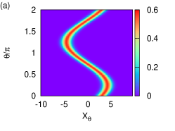
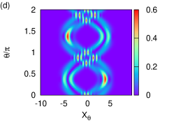
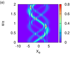
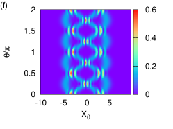
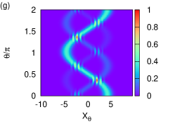
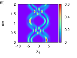
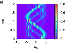
Figure 1: Tomograms of an initial CS with $\alpha=\sqrt{10}e^{i\pi/4}$ for a cubic Hamiltonian at instants (a) $0$ and $T_{rev}$, (b) $T_{rev}/2$, (c) $T_{rev}/3$, (d) $T_{rev}/4$, (e) $T_{rev}/5$, (f) $T_{rev}/6$, (g) $T_{rev}/9$, (h) $T_{rev}/12$, and (i) $T_{rev}/15$.

These features follow from the properties of the unitary time evolution operator corresponding to this system. It is known for instance that for the simpler system with Hamiltonian ${a^{\dagger}}^{2}a^{2}$ the number of subpackets $p$ of a wave packet at an instant of fractional revival $T_{rev}/p$ is a consequence of the periodicity of the unitary time evolution operator which can be Fourier decomposed at that instant in the form

$$U\left(T_{rev}/p\right)=\sum_{m=0}^{p-1}f_{m}\exp\left(-\frac{2\pi\rmi m}{p}N\right),$$ (12)

where $f_{m}$ is a Fourier coefficient. As a consequence, an initial state $\ket{\alpha}$ evolves to a superposition of $p$ coherent states at that instant [23].

While the system at hand is more complicated, the full revival at $T_{rev}/3$ is a simple consequence of the fact that $n(n-1)(n-2)/3$ is even $\forall\,n\epsilon\mathbb{N}$. Here, $N\ket{n}=n\ket{n}$, with $\{\ket{n}\}$ denoting the photon number basis. Hence corresponding to an initial state $\ket{\psi(0)}=\sum_{m=0}^{\infty}c_{n}\ket{n}$, the state at instant $T_{rev}/3$ is

$$\ket{\psi(T_{rev}/3)} =U(T_{rev}/3)\ket{\psi(0)}$$

$$=\sum_{n=0}^{\infty}\rme^{-\rmi\pi n(n-1)(n-2)/3}c_{n}\ket{n}$$

$$=\ket{\psi(0)}.$$

An analysis of the properties of the time evolution operator would, in principle, explain the appearance of a specific number of strands in the tomogram at different instants $T_{rev}/l$. However accounting for the number of strands in a tomogram is not always straightforward in this case, in contrast to the Kerr-like system.

We are now in a position to investigate tomogram patterns for the full Hamiltonian

$$H=(\chi_{1}a^{\dagger 2}a^{2}+\chi_{2}a^{\dagger 3}a^{3}).$$ (13)

In this case,

$$T_{rev}=\pi\,\mathrm{LCM}\left(\frac{1}{\chi_{1}},\frac{1}{\chi_{2}}\right).$$ (14)

As before, we proceed to examine tomogram patterns at different instants of time. If the ratio $\chi_{1}/\chi_{2}$ is irrational, revivals are absent and the generic tomogram at any instant is blurred. This is illustrated in figure 2 for an initial CS with $\alpha=\sqrt{10}\exp(i\pi/4)$ with $\chi_{1}=2$, and $\chi_{2}=\sqrt{2}$ at $t=\pi/\chi_{2}$.

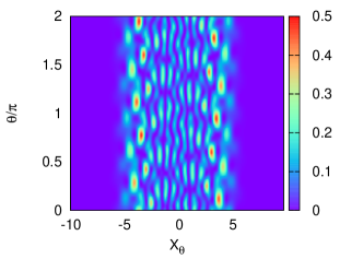
Figure 2: Tomogram of an initial CS with $\alpha=\sqrt{10}e^{i\pi/4}$, $\chi_{1}=2.0$ and $\chi_{2}=\sqrt{2}$ at $t=\pi/\chi_{2}$.

For rational $\chi_{1}/\chi_{2}$ revivals and fractional revivals are seen. Fractional revivals occur at instants $T_{rev}/l$ as before, but the corresponding tomogram patterns are sensitive to the ratio $\chi_{1}/\chi_{2}$. We expect that for a given $l$ the tomogram will have $l$ strands as a consequence of the Kerr-like term in $H$. While this is one possibility, the effect of the cubic term in $H$ allows for the possibility of other tomogram patterns. We illustrate this for an initial CS with Hamiltonian $H$ and $\alpha=\sqrt{10}\exp(i\pi/4)$ in figures 3, 4, and 5. At $t=T_{rev}/2$, apart from the two-strand tomogram for $\chi_{1}=1$ and $\chi_{2}=2$, one of the other possibilities is a four-strand tomogram for $\chi_{1}=1$ and $\chi_{2}=3$ (figure 3). Similarly at $t=T_{rev}/3$, the tomogram has three strands for $\chi_{1}=1$ and $\chi_{2}=2$ and a single strand similar to the tomogram of a CS for $\chi_{1}=3$ and $\chi_{2}=4$ (figure 4). At $t=T_{rev}/4$ three specimen tomograms which are distinctly different from each other are shown in figures 5 (a)-(c) for $\chi_{1}=1$ and $\chi_{2}=2$, $\chi_{1}=1$ and $\chi_{2}=3$ and $\chi_{1}=1$ and $\chi_{2}=4/3$ respectively.

These features can be explained on a case by case basis as before by examining the periodicity properties of the unitary time evolution operator at appropriate instants. It is however evident that the simple inference that an $l$-subpacket fractional revival is associated with an $l$-strand tomogram alone does not hold when more than one time scale is involved in the Hamiltonian, and there can be several tomograms possible at a given instant depending on the interplay between the different time scales in the system.

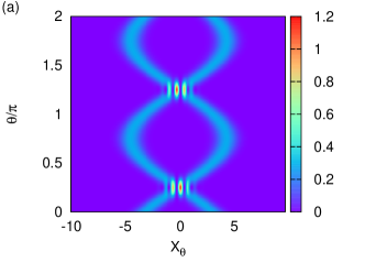
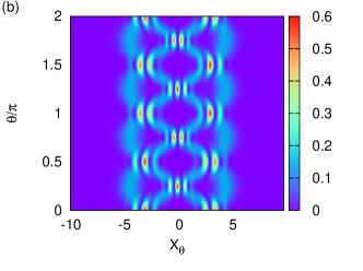
Figure 3: Tomograms of an initial CS with $\alpha=\sqrt{10}e^{i\pi/4}$ at $t=\frac{T_{rev}}{2}$ for (a) $\chi_{1}=1$ and $\chi_{2}=2$ and (b) $\chi_{1}=1$ and $\chi_{2}=3$.

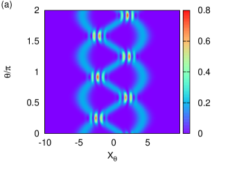
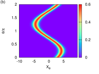
Figure 4: Tomograms of an initial CS with $\alpha=\sqrt{10}e^{i\pi/4}$ at $t=\frac{T_{rev}}{3}$ for (a) $\chi_{1}=1$ and $\chi_{2}=2$ and (b) $\chi_{1}=3$ and $\chi_{2}=4$.

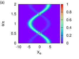
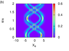
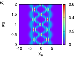
Figure 5: Tomograms of an initial CS with $\alpha=\sqrt{10}e^{i\pi/4}$ at $t=\frac{T_{rev}}{4}$ for (a) $\chi_{1}=1$ and $\chi_{2}=2$, (b) $\chi_{1}=1$ and $\chi_{2}=3$, and (c) $\chi_{1}=1$ and $\chi_{2}=4/3$.

2.2 Squeezing and higher-order squeezing

We now proceed to examine the squeezing and higher-order squeezing properties of the system with Hamiltonian $H$. Once again, our aim is to identify and assess these nonclassical effects directly from the tomogram without attempting to reconstruct the state of the system at any instant of time. The extent of quadrature squeezing at a given instant is essentially determined by the numerical value of the variance of the quadrature observables. The state of the system is said to be squeezed in $x$ if the variance $(\Delta x)^{2}=\langle(x-\langle{x}\rangle)^{2}\rangle$ is less than the variance of $x$ in a CS $\ket{\alpha}$. Generalization of this definition to include higher-order squeezing allows for two possibilities. Hong-Mandel squeezing of order $2q$ in $x$ requires that $\langle(x-\langle{x}\rangle)^{2q}\rangle$ for the given state is less than the corresponding expectation value for the CS. Here $q=2,3,\dots$. We will estimate the extent of Hong-Mandel squeezing by calculating the central moments of the probability distribution corresponding to the appropriate quadrature. For example, if we wish to determine the extent of second-order Hong-Mandel squeezing in the $x$ quadrature, we simply calculate the fourth central moment of a horizontal cut of the tomogram at $\theta=0$. Note that for $q=1$, Hong-Mandel squeezing is identical to quadrature squeezing.

Hillery type squeezing of order $q$ corresponds to squeezing in either of the pair of operators $Z_{1}=(a^{q}+{a^{\dagger}}^{q})/\sqrt{2}$ and $Z_{2}=(a^{q}-{a^{\dagger}}^{q})/\sqrt{2}\,\rmi$, where $q=2,3,\dots$. A useful quantifier $D_{q}$ of $q$th-power squeezing in $Z_{1}$ for instance, is defined [24] in terms of the commutator $[a^{q},{a^{\dagger}}^{q}]=F_{q}(N)$ as

$$D_{q}=\frac{\langle(\Delta Z_{1})^{2}\rangle-|F_{q}(N)|}{|{F_{q}(N)}|}.$$ (15)

where $(\Delta Z_{1})^{2}$ is the variance in $Z_{1}$. A similar definition holds for $q$th power squeezing in $Z_{2}$. We note that $F_{q}(N)$ is a polynomial function of order $(q-1)$ in $N$. A state is $q$th-power squeezed if $-1\leq D_{q}<0$. It is clear that $Z_{1}$ and $Z_{2}$ cannot be obtained in a straightforward manner from the tomogram as they involve terms with products of powers of different rotated quadratures and hence cannot be assigned probability distributions directly from a set of tomograms.

However an illustrative treatment of the problem of expressing the expectation value of a product of moments of creation and destruction operators in terms of the tomogram $w$ and Hermite polynomials [25] leads to the result

$$\braket{a^{\dagger k}a^{l}} =C_{kl}\sum_{m=0}^{k+l}\exp\left(-\rmi(k-l)\left(\frac{m\pi}{k+l+1}\right)\right)$$ (16)

$$\int_{-\infty}^{\infty}\rmd X_{\theta}\ w\left(X_{\theta},\ \frac{m\pi}{k+l+1}\right)H_{k+l}\left(X_{\theta}\right),$$

where

$$C_{kl}=\frac{k!l!}{(k+l+1)!\sqrt{2^{k+l}}}.$$

This form is readily amenable to numerical computations. We therefore need to consider $(k+l+1)$ values of the tomogram variable $\theta$ in order to calculate a moment of order $(k+l)$. In a single tomogram, this amounts to using $(k+l+1)$ probability distributions $w(X_{\theta}$) corresponding to these chosen values of $\theta$, in order to calculate the squeezing parameter $D_{q}$ from the tomogram without resorting to detailed state reconstruction. As the system evolves in time, the extent of squeezing at various instants are determined from the instantaneous tomograms in this manner.

For the squeezed vacuum, $\ket{\alpha}$ and $\ket{\alpha,1}$ we have verified that the variance and hence the Hong-Mandel (equivalently Hillery type squeezing) properties inferred directly from tomograms are in excellent agreement with corresponding results obtained analytically by calculating the variance from the state. We have also computed $\langle(\Delta x)^{4}\rangle$ (equivalently the higher-order Hong-Mandel squeezing parameter) directly from the tomogram for initial states $\ket{\alpha}$ and $\ket{\alpha,1}$ evolving under the Kerr-like Hamiltonian and the cubic Hamiltonian ${a^{\dagger}}^{3}a^{3}$, setting $\alpha=1$ in both cases without loss of generality (see figures 6(a) and (b)). From these figures it is evident that independent of the precise nature of the initial field state $\langle(\Delta x)^{4}\rangle$ oscillates more rapidly in the case of the cubic Hamiltonian compared to the Kerr-like Hamiltonian. Earlier these squeezing properties have been investigated for an initial CS and PACS evolving under a Kerr-like Hamiltonian by calculating $\langle(\Delta x)^{4}\rangle$ explicitly for the state at different times [3]. Our results from the tomograms for the Kerr-like Hamiltonian are in excellent agreement with these.

We have also examined the manner in which the squeezing properties depend on the numerical value of $\alpha$, directly from the relevant tomograms. For real $\alpha$ in the range $0$ to $\sqrt{3}$ we have plotted $D_{1}$ the quantifier of the extent of squeezing versus $\nu=|\alpha|^{2}$ at the instant $T_{rev}/2$ for an initial CS evolving under both the Kerr and cubic Hamiltonians (figure 7(a)). It is evident that the state is squeezed for a larger range of values of $\nu$ in the case of the Kerr-like Hamiltonian than for the cubic Hamiltonian. Further the extent of squeezing as measured by the numerical value of $D_{1}$ is more for a given $\nu$ in the former case as compared to the latter.

For an initial state $\ket{\alpha,1}$ we have computed the extent of higher-order Hillery type squeezing from the tomograms over the range $0\leq\nu\leq 3$, at $T_{rev}/2$ for both Hamiltonians. While $D_{2}$ is not negative for any $\nu$ in this range for the cubic Hamiltonian, it becomes negative for $\nu\geq 0.8$ approximately for the Kerr-like Hamiltonian (figure 7(b)). In contrast $\langle(\Delta x)^{4}\rangle$ is not negative in both cases over this range of values of $\nu$ (figure 7(c)).

Figure 6: Hong-Mandel squeezing as a function of scaled time $t/T_{rev}$ for initial states (a)$\ket{\alpha}$ and (b)$\ket{\alpha,1}$ with $\alpha=1$. The solid (dashed) line corresponds to the Kerr (respectively cubic) Hamiltonian.

Figure 7: (a) $D_{1}$ for initial $\ket{\alpha}$, (b) $D_{2}$ for initial $\ket{\alpha,1}$, and (c) $\langle(\Delta x)^{4}\rangle$ for initial $\ket{\alpha,1}$ versus $\nu$ for real $\alpha$ at instant $\frac{T_{rev}}{2}$. The solid (dashed) line corresponds to the Kerr (respectively cubic) Hamiltonian.

3 The double-well BEC: A tomographic approach

3.1 The Revival Phenomena

We now proceed to examine nonclassical effects in a BEC condensed in a double-well potential. The effective Hamiltonian of this bipartite system is  [26]

$$H_{bec}=\omega_{0}N_{tot}+\omega_{1}(a^{\dagger}a-b^{\dagger}b)+U_{ab}N_{tot}^{2}-\lambda(a^{\dagger}b+ab^{\dagger}).$$ (17)

$(a,a^{\dagger})$ and $(b,b^{\dagger})$ are the boson annihilation and creation operators corresponding to the two subsystems $A$ and $B$ which comprise the atomic species condensed in the two wells. They satisfy $[a,a^{\dagger}]=1$, $[b,b^{\dagger}]=1$ with all other commutators vanishing. Here, $N_{tot}=(a^{\dagger}a+b^{\dagger}b)$ and $U_{ab}$ is the strength of the nonlinearity. It is convenient to define the effective interaction strength by the parameter $\lambda_{1}=\sqrt{\omega_{1}^{2}+\lambda^{2}}$. It is easy to see that $[H_{bec},N_{tot}]=0$.

Before we examine revivals and squeezing phenomena in this system by investigating relevant tomograms, we recall that we now have two quadrature operators to consider, one for each subsystem. The tomogram is therefore denoted by $w(X_{\theta_{1}},\theta_{1};X_{\theta_{2}},\theta_{2})$ with subscripts $1$ and $2$ corresponding to subsystems $A$ and $B$ respectively.

Analogous to the single-mode example we now consider a pure state $\ket{\psi}$ expanded in the Fock bases $\{\ket{m}\}$, $\{\ket{n}\}$ corresponding to subsystems A and B respectively as $\ket{\psi}=\sum_{m,n=0}^{\infty}c_{mn}\ket{m;n}$ , where $\ket{m;n}$ is a short-hand notation for $(\ket{m}\otimes\ket{n})$ and $c_{mn}$ are the expansion coefficients.

It is straightforward to extend the procedure for expressing the optical tomogram in the single-mode example in terms of Hermite polynomials to a generic bipartite system whose subsystems are infinite-dimensional. We can see that analogous to (10), in this case we have

$$w(X_{\theta_{1}},\theta_{1};X_{\theta_{2}},\theta_{2})=\frac{\exp(-X_{\theta_{1}}^{2}-X_{\theta_{2}}^{2})}{\pi}$$

$$\times\left|\sum_{m,n=0}^{\infty}\frac{c_{mn}\rme^{-\rmi(m\theta_{1}+n\theta_{2})}}{\sqrt{m!n!2^{m+n}}}H_{m}(X_{\theta_{1}})H_{n}(X_{\theta_{2}})\right|^{2}.$$ (18)

The tomograms corresponding to the two subsystems (reduced tomograms) are given by

$$w_{1}(X_{\theta_{1}},\theta_{1})=\int_{-\infty}^{\infty}w(X_{\theta_{1}},\theta_{1};X_{\theta_{2}},\theta_{2})\rmd X_{\theta_{2}},$$ (19)

for any fixed value of $\theta_{2}$ and

$$w_{2}(X_{\theta_{2}},\theta_{2})=\int_{-\infty}^{\infty}w(X_{\theta_{1}},\theta_{1};X_{\theta_{2}},\theta_{2})\rmd X_{\theta_{1}}$$ (20)

for any fixed value of $\theta_{1}$.

We denote by $\ket{\alpha_{a}}$ (respectively $\ket{\alpha_{b}}$) the CS formed from the condensate corresponding to subsystem A (respectively B) and by $\ket{\alpha_{a},1}$ (respectively $\ket{\alpha_{b},1}$) a 1-boson added CS corresponding to subsystem A (respectively B). The initial states considered by us are factored product states of the form $\ket{\alpha_{a}}\otimes\ket{\alpha_{b}}$ (denoted by $\ket{\psi_{00}}$), $\ket{\alpha_{a},1}\otimes\ket{\alpha_{b},1}$( denoted by $\ket{\psi_{11}}$) and $\ket{\alpha_{a},1}\otimes\ket{\alpha_{b}}$ (denoted by $\ket{\psi_{10}}$).

The state at a subsequent time $t$ is entangled in general and corresponding to the initial state $\ket{\psi_{00}}$ we have [26]

$$\ket{\psi_{00}(t)} =\exp(-n/2)\sum_{p,q=0}^{\infty}\frac{(\alpha(t))^{p}(\beta(t))^{q}}{\sqrt{p!q!}}$$ (21)

$$\exp(-\rmi t(\omega_{0}(p+q)+U_{ab}(p+q)^{2}))\ket{p;q}.$$

Here,

$$\alpha(t)=\alpha_{a}\cos(\lambda_{1}t)+\rmi\frac{\sin(\lambda_{1}t)}{\lambda_{1}}\left(\lambda\alpha_{b}-\omega_{1}\alpha_{a}\right),\\$$

$$\beta(t)=\alpha_{b}\cos(\lambda_{1}t)+\rmi\frac{\sin(\lambda_{1}t)}{\lambda_{1}}\left(\lambda\alpha_{a}+\omega_{1}\alpha_{b}\right),$$

and $n=({|\alpha_{a}|}^{2}+{|\alpha_{b}|}^{2})$ [26].

We can use a similar procedure to obtain $\ket{\psi_{10}(t)}$ and $\ket{\psi_{11}(t)}$. We have

$$\ket{\psi_{10}(t)}=\frac{1}{d_{10}} \left(a^{\dagger}\lambda_{1}\cos(\lambda_{1}t)+\rmi(\lambda b^{\dagger}-\omega_{1}a^{\dagger})\sin(\lambda_{1}t)\right)$$ (22)

$$\times\exp(-\rmi U_{ab}(2N+1)t)\ket{\psi_{00}(t)},$$

and

$$\ket{\psi_{11}(t)}= \frac{1}{d_{11}}\biggl{(}2\omega_{1}^{2}\,a^{\dagger}b^{\dagger}+\omega_{1}\lambda\left(a^{\dagger 2}-b^{\dagger 2}\right)$$ (23)

$$+\cos(2\lambda_{1}t)\left(2\lambda^{2}\,a^{\dagger}b^{\dagger}-\omega_{1}\lambda\left(a^{\dagger 2}-b^{\dagger 2}\right)\right)$$

$$+\rmi\sin(2\lambda_{1}t)\lambda\lambda_{1}(a^{\dagger 2}+b^{\dagger 2})\biggr{)}$$

$$\times\exp(-4\rmi U_{ab}(N+1)t)\ket{\psi_{00}(t)}.$$

Here $d_{10}=\lambda_{1}\exp(\rmi\omega_{0}t)\sqrt{1+{|\alpha_{a}|}^{2}}$ and $d_{11}=2\lambda_{1}^{2}\exp(2\rmi\omega_{0}t)\sqrt{1+{|\alpha_{a}|}^{2}}\sqrt{1+{|\alpha_{b}|}^{2}}$.

We have obtained a form for the density matrix which is very useful in numerical computations. The salient steps in the calculation of the density matrix $\rho_{m_{1},m_{2}}$ corresponding to the factored product state $\ket{\alpha_{a},m_{1}}\otimes\ket{\alpha_{b},m_{2}}$ for any positive integer value of $m_{1}$ and $m_{2}$ are outlined in the Appendix. We have shown there that $\rho_{m_{1},m_{2}}$ can be expressed in terms of an operator $M_{m_{1},m_{2}}(t)$ and $\ket{\psi_{00}(t)}$ as

$$\rho_{m_{1},m_{2}}(t)=M_{m_{1},m_{2}}(t)\ket{\psi_{00}(t)}\bra{\psi_{00}(t)}M^{\dagger}_{m_{1},m_{2}}(t).$$ (24)

Defining $p_{max}=(k+m_{2}-l)$ and $q_{max}=(l+m_{1}-k)$ we have

$$M_{m_{1},m_{2}}(t)=\frac{1}{\kappa}\biggl{[}\sum_{k=0}^{m_{1}}\sum_{l=0}^{m_{2}}\sum_{p=0}^{p_{max}}\sum_{q=0}^{q_{max}}(-1)^{k-p}{m_{1}\choose k}{m_{2}\choose l}$$

$$\hskip 20.00003pt{p_{max}\choose p}{q_{max}\choose q}\exp(-\rmi\lambda_{1}t(2(k-l)+m_{2}-m_{1}))$$

$$\hskip 20.00003pt(\cos(\gamma/2))^{(k+l+p+q)}(\sin(\gamma/2))^{(2(m_{1}+m_{2})-(k+l+p+q))}$$

$$\hskip 20.00003pta^{\dagger(p+q_{max}-q)}b^{\dagger(q+p_{max}-p)}\biggr{]}\exp(-\rmi\omega_{0}t(m_{1}+m_{2}))$$

$$\times\exp(-\rmi U_{ab}t(m_{1}+m_{2})(2N_{tot}+m_{1}+m_{2})).$$ (25)

Here $\kappa=\sqrt{m_{1}!L_{m_{1}}(-{|\alpha_{a}|}^{2})m_{2}!L_{m_{2}}(-{|\alpha_{b}|}^{2})}$ and $\gamma=\cos^{-1}(\omega_{1}/\lambda_{1})$. $L_{m}$ are the Laguerre polynomials which appear in the normalization of $\ket{\alpha,m}$. This expression for the general density matrix can be easily seen to reduce to the forms needed in our case where the states are $\ket{\psi_{00}(t)}$, $\ket{\psi_{11}(t)}$ and $\ket{\psi_{10}(t)}$.

We now proceed to examine the revival phenomena by studying appropriate tomograms in this case. A straightforward calculation reveals that full and fractional revivals occur provided $\omega_{0}=mU_{ab}$, $\lambda_{1}=m^{\prime}U_{ab}$, $m,m^{\prime}\in\mathbb{Z}$, and $(m+m^{\prime})$ is odd. Fractional revivals occur at fractions of the revival period $T_{rev}$ (which is equal to $\pi/U_{ab}$). This follows (similar to the single-mode case) from the periodicity property of $\exp(-iU_{ab}N_{tot}^{2})$. For instance, we can easily show that an initial state $\ket{\psi_{00}}$ evolves at an instant $\pi/(sU_{ab})$ ($s$: even integer) to

$$\ket{\psi_{00}(\pi/sU_{ab})}= \sum_{j=0}^{s-1}a_{j}\ket{\alpha(\pi/sU_{ab})\rme^{-\rmi\pi(m+2j)/s}}$$ (26)

$$\otimes\ket{\beta(\pi/sU_{ab})\rme^{-\rmi\pi(m+2j)/s}},$$

If $s$ is an odd integer,

$$\ket{\psi_{00}(\pi/sU_{ab})}= \sum_{j=0}^{s-1}b_{j}\ket{\alpha(\pi/sU_{ab})\rme^{-\rmi\pi(m+2j+1)/s}}$$ (27)

$$\otimes\ket{\beta(\pi/sU_{ab})\rme^{-\rmi\pi(m+2j+1)/s}}.$$

Note that $\alpha\left(\pi/(sU_{ab})\right)$ and $\beta\left(\pi/(sU_{ab})\right)$ are obtained from (3.1) and (3.1).

We recall that in the single-mode system the occurrence of full and fractional revivals are related to the presence of distinct strands in the tomogram. In this bipartite system however, the tomogram is a 4-dimensional hypersurface. Hence we need to consider appropriate sections to identify and examine nonclassical effects. The 2-dimensional section ($X_{\theta_{2}}$ - $X_{\theta_{1}}$) obtained by setting $\theta_{1}$ and $\theta_{2}$ constant is a natural choice for investigating not only revival phenomena but also squeezing properties. In contrast to the single-mode case where strands appear in the tomograms these sections are characterized by ‘blobs’ at instants of fractional revivals. The number of blobs gives the number of subpackets in the wave packet.

Although $\ket{\alpha}$ is expanded as an infinite superposition of photon number states, in practice, a numerical computation can be carried out using only a large but finite sum of these basis states. An alternative is to use truncated coherent state(TCS) [27] instead of the standard CS. The latter are defined as

$${\ket{\alpha}}_{tcs}=\frac{1}{\sum_{n=0}^{N_{max}}(|\alpha|^{2n}/n!)}\sum_{p=0}^{N_{max}}\frac{\alpha^{p}}{\sqrt{p!}}\ket{p}.$$ (28)

where $N_{max}$ is a sufficiently large but finite integer. We have worked with an initial state $\ket{\alpha_{a}}_{tcs}\otimes\ket{\alpha_{b}}_{tcs}$ instead of $\ket{\psi_{00}}$ and verified that as this state evolves under $H_{bec}$ the revival phenomena and squeezing properties mimic that of $\ket{\psi_{00}}$ remarkably well. Hence we have used initial states $\ket{\psi_{00}}$, $\ket{\psi_{10}}$ and $\ket{\psi_{11}}$ for our numerical computations. We set $\theta_{1}=\theta_{2}=0$, $\omega_{0}=10$, $\omega_{1}=3$, $\lambda=4$, $U_{ab}=1$, and $\alpha_{a}=\alpha_{b}=10$ in figures 8 (a)-(d) where we present tomograms corresponding to different fractional revivals for the initial state $\ket{\psi_{00}}$. At instants $T_{rev}/4$, $T_{rev}/3$ and $T_{rev}$ (figures 8(a), (b) and (d) respectively) we see 4, 3 and a single blob in the tomogram along with interference patterns as expected for this choice of values of $\lambda_{1}$ and $\omega_{0}$ for they satisfy the conditions $\omega_{0}=mU_{ab}$, $\lambda_{1}=m^{\prime}U_{ab}$, $m,m^{\prime}\in\mathbb{Z}$, and $(m+m^{\prime})$ is odd, necessary for the revival phenomena to occur. However in figure 8(c) corresponding to the instant $T_{rev}/2$ blobs are absent and we merely see interference patterns. This is primarily due to the specific choice of real values of $\alpha_{a}$ and $\alpha_{b}$ as explained below. At the instant $T_{rev}/2$ it follows from (21) that the state of the system can be expanded in terms of superpositions of factored products of CS corresponding to $A$ and $B$ as

$$\ket{\psi_{00}(T_{rev}/2)}= \frac{(1-\rmi)}{2}\ket{{-2\rmi}/{\sqrt{10}}}\otimes\ket{{-14\rmi}/{\sqrt{10}}}$$ (29)

$$+\frac{(1+\rmi)}{2}\ket{{2\rmi}/{\sqrt{10}}}\otimes\ket{{14\rmi}/{\sqrt{10}}}.$$

It is now straightforward to see why the interference patterns alone appear in the tomogram, as a simple calculation gives

$$|\psi_{00}(X_{10},X_{20})|^{2}=|\langle X_{10},0;X_{20},0|\psi_{00}(T_{rev}/2)\rangle|^{2}$$

$$=\frac{1}{\pi}\rme^{-(X_{10}^{2}+X_{20}^{2})}\left(1-\sin(4(X_{10}+7X_{20})/\sqrt{5})\right).$$ (30)

Here $X_{10}$ denotes $X_{\theta_{1}}$ for $\theta_{1}=0$ and $X_{20}$ denotes $X_{\theta_{2}}$ for $\theta_{2}=0$. In contrast, it can be seen that if $\alpha_{a}$ and $\alpha_{b}$ were chosen to be generic complex numbers two blobs together with the interference pattern would be seen to appear at $T_{rev}/2$ also.

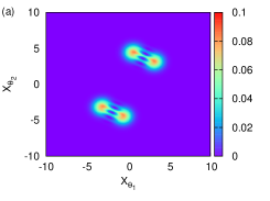
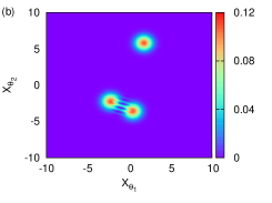
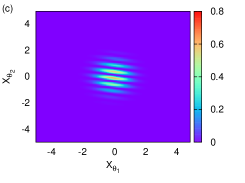
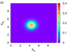
Figure 8: Sections of the optical tomogram for $\theta_{1}=\theta_{2}=0$ at instants of fractional revivals (a)$T_{rev}/4$, (b)$T_{rev}/3$, (c)$T_{rev}/2$, and (d)$T_{rev}$. $\alpha_{a}=\alpha_{b}=\sqrt{10}$, for an initial state $\ket{\psi_{00}}$.

Similar results hold in the case of initial states $\ket{\psi_{11}}$ and $\ket{\psi_{10}}$.

3.2 Squeezing and higher-order squeezing of the condensate

The extent of Hong-Mandel squeezing is simply obtained as in the single-mode example, by calculating the central moments of the probability distribution corresponding to the quadrature. We examine two-mode squeezing by evaluating appropriate moments of the quadrature variable $\eta=(a+a^{\dagger}+b+b^{\dagger})/2\sqrt{2}$. These are obtained from the $\theta_{1}=\theta_{2}=0$ section of the tomogram as the system evolves in time. These moments have also been obtained by explicit calculation of the relevant expectation values of $\eta$ in the state of the system at different times. In both cases the initial state considered is $\ket{\psi_{00}}$. In figures 9 (a)-(d), the variance and $2q$-order moments for $q=1,2,3$ and $4$ obtained both from the states and directly from the tomogram are plotted as a function of time. It is evident that they are in excellent agreement with each other at all instants. The horizontal line in each figure denotes the value below which the state is squeezed. For all values of $q$ considered, the state is squeezed (higher-order squeezed) in the neighborhood of revivals, and the actual magnitude at various instants is considerably sensitive to the value of $q$ as expected. We have also verified that the extent of this Hong-Mandel squeezing depends on the magnitude of $\alpha_{a}$ and $\alpha_{b}$ at various instants of time.

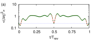
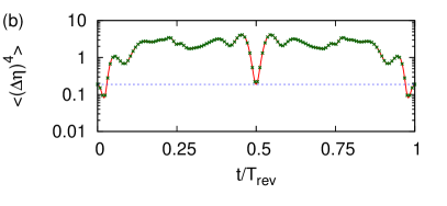
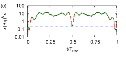
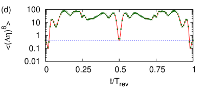
Figure 9: $2q$-order moment of $\eta=(a+a^{\dagger}+b+b^{\dagger})/2\sqrt{2}$ versus $t/T_{rev}$ with $|\alpha_{a}|=|\alpha_{b}|=1$, for (a) $q=1$, (b) $q=2$, (c) $q=3$, and (d) $q=4$. Moments obtained directly from the tomogram are denoted by green crosses and those from the state by the red solid curve. The horizontal line denotes the moment corresponding to the CS.

For numerical computation of the Hillery type higher-order squeezing recall that in the single-mode case we used the expression [25] for moments of the creation and destruction operators in terms of the tomogram and Hermite polynomials given by

$$\braket{a^{\dagger k}a^{l}} =C_{kl}\sum_{m=0}^{k+l}\exp\left(-\rmi(k-l)\left(\frac{m\pi}{k+l+1}\right)\right)$$ (31)

$$\int_{-\infty}^{\infty}\rmd X_{\theta}\ w\left(X_{\theta},\frac{m\pi}{k+l+1}\right)H_{k+l}\left(X_{\theta}\right),$$

where

$$C_{kl}=\frac{k!l!}{(k+l+1)!\sqrt{2^{k+l}}}.$$

A straightforward extension to the two-mode system gives us the required expression

$$\langle a^{\dagger k}a^{l} b^{\dagger m}b^{n}\rangle=c_{klmn}\sum_{p=0}^{k+l}\sum_{q=0}^{m+n}\exp\left(-\rmi(k-l)\theta_{1p}\right)$$ (32)

$$\exp\left(-\rmi(m-n)\theta_{2q}\right)\int_{-\infty}^{+\infty}\rmd X_{\theta_{1p}}\int_{-\infty}^{+\infty}\rmd X_{\theta_{2q}}$$

$$w\left(X_{\theta_{1p}},\theta_{1p};X_{\theta_{2q}},\theta_{2q}\right)H_{k+l}(X_{\theta_{1p}})H_{m+n}(X_{\theta_{2q}}).$$

Here

$$c_{klmn}=\frac{k!l!m!n!}{(k+l+1)!(m+n+1)!\sqrt{2^{k+l+m+n}}},$$

$\theta_{1p}=\frac{p\pi}{k+l+1}$, and $\theta_{2q}=\frac{q\pi}{m+n+1}$. Note that $(k+l+1)(m+n+1)$ gives the number of 2- dimensional slices of the tomogram that are required to calculate $\langle a^{\dagger k}a^{l}b^{\dagger m}b^{n}\rangle$.

In figures 10 (a)-(d) $D_{q}(t)$ obtained both from the states and directly from the tomogram for an initial state $\ket{\psi_{00}}$ are compared and seen to be in excellent agreement. It is clear from the figures that for higher values of $q$ there are more instants of time when higher-order squeezing occurs as expected from the fact that more cross terms involving the creation and destruction operators arise with increase in $q$.

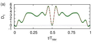
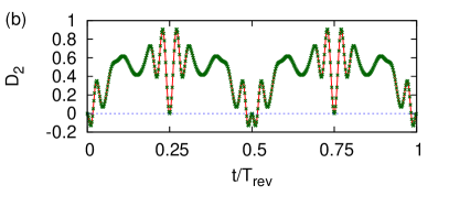
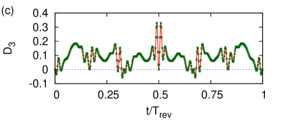
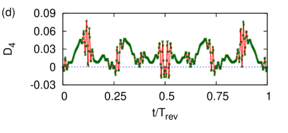
Figure 10: $D_{q}(t)$ versus $t/T_{rev}$ for $|\alpha_{a}|=|\alpha_{b}|=1$ and (a) $q=1$, (b) $q=2$, (c) $q=3$, and (d)$q=4$. The squeezing parameter obtained directly from the tomogram is denoted by green crosses and that from the state by the red solid curve. The horizontal line corresponds to $D_{q}(t)=0$.

We have also verified that both the Hong-Mandel and Hillery type squeezing and higher-order squeezing parameters obtained from tomograms and from expectation values of appropriate operators for the initial states $\ket{\psi_{10}}$ and $\ket{\psi_{11}}$ were equal to each other at all instants between $t=0$ and $T_{rev}$.

3.3 Subsystem entropies from tomograms

This bipartite system provides an ideal framework for investigating a subsystem’s nonclassical properties from the tomogram. We are primarily interested in computing the quantum information entropy and entropic squeezing properties of the subsystem as it evolves in time. Further, we extract the subsystem von Neumann entropy from the tomogram to quantify the extent of entanglement between the two condensates trapped in the double well. (Without loss of generality we have considered subsystem $A$ by setting $\theta_{2}=0$, and integrating over the full range of $X_{\theta_{2}}$ to obtain $w(X_{\theta_{1}},\theta_{1})$).

In order to examine entropic squeezing we have further set $\theta_{1}=0$ and investigated the manner in which $S_{0}$ (the information entropy of subsystem $A$ given by $-\int_{-\infty}^{\infty}\rmd X_{\theta_{1}}\,w_{1}\,\log w_{1}$) varies as the system evolves in time. (Here $w_{1}$ denotes $w(X_{\theta_{1}})$). This information entropy has been plotted in figures 11 (a)-(c) for initial states $\ket{\psi_{00}}$, $\ket{\psi_{10}}$ and $\ket{\psi_{11}}$ respectively. The horizontal line in these figures denotes the numerical value below which entropic squeezing occurs in the quadrature considered. We see that entropic squeezing occurs close to $t=0$ and $T_{rev}$. At other instants the entropy is significantly higher in the case of initial states $\ket{\psi_{10}}$ and $\ket{\psi_{11}}$ compared to initial ideal coherence. This feature is very prominent close to $T_{rev}/2$. Further, comparing (b) and (c) it is clear that $S_{0}$ is larger at all instants if both subsystems depart from coherence initially, compared to the case where one of them displays initial coherence.

Figure 11: Quantum information entropy $S_{0}$ versus $t/T_{rev}$ for initial states (a) $\ket{\psi_{00}}$, (b) $\ket{\psi_{10}}$, and (c) $\ket{\psi_{11}}$ for $\alpha_{a}=\alpha_{b}=1$.

Figures 12 (a), (b) and (d) show the variation of $S_{0}$ corresponding to subsystem $A$ with $|\alpha_{a}|^{2}$ and $|\alpha_{b}|^{2}$, at $T_{rev}/2$, for initial states $\ket{\psi_{00}}$, $\ket{\psi_{10}}$ and $\ket{\psi_{11}}$ respectively. Figure 12 (c) corresponds to the entropy of subsystem $B$ for an initial state $\ket{\psi_{10}}$. This facilitates comparison of the features in figures 12 (b) and (c) where for the same asymmetric initial state the two subsystems examined are different. It is evident that $S_{0}$ corresponding to $A$ is not squeezed while that corresponding to $B$ exhibits squeezing for some values of $\alpha_{a}$ and $\alpha_{b}$. The role played by the asymmetry in the initial states of the two subsystems is thus clearly brought out in these figures. It is also clear from figures 12 (a)-(d) that entropic squeezing is more if the initial states of the subsystems are coherent.

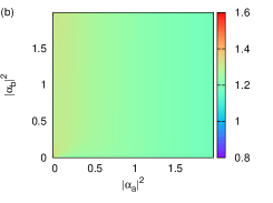
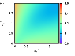
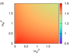
Figure 12: Quantum information entropy $S_{0}$ versus $|\alpha_{a}|^{2}$ and $|\alpha_{b}|^{2}$ at $T_{rev}/2$ for initial states (a) $\ket{\psi_{00}}$, (b) and (c) $\ket{\psi_{10}}$, and (d) $\ket{\psi_{11}}$.

Finally, we identify the extent of entanglement between $A$ and $B$ in terms of quantities which are accessible from the tomogram. ‘Information transfer’ between $A$ and $B$ takes place because of the interaction and consequent entanglement between them. Hence we investigate the possibility of defining a quantum analogue of mutual information between two classical systems which could be used as an entanglement measure. We recall that $w_{1}$ is independent of the value of $\theta_{2}$ and hence the information entropy

$$S(\theta_{1})=-\int_{-\infty}^{\infty}\rmd X_{\theta_{1}}\,w_{1}\,\log w_{1},$$ (33)

is also independent of the value of $\theta_{2}$. A similar statement holds for $S(\theta_{2})$. (Recall that $S_{0}$ is merely $S_{\theta_{1}=0}$.) However,

$$S(\theta_{1},\theta_{2})=-\int_{-\infty}^{\infty}\rmd X_{\theta_{1}} \int_{-\infty}^{\infty}\rmd X_{\theta_{2}}\,w(X_{\theta_{1}},\theta_{1};X_{\theta_{2}},\theta_{2})$$ (34)

$$\log w(X_{\theta_{1}},\theta_{1};X_{\theta_{2}},\theta_{2}).$$

clearly depends on the values of both $\theta_{1}$ and $\theta_{2}$.

We can now define, following the notation in [28]

$$S(\theta_{1}:\theta_{2})=S(\theta_{1})+S(\theta_{2})-S(\theta_{1},\theta_{2}).$$ (35)

$S(\theta_{1}:\theta_{2})$ is analogous to the classical mutual information. We can now get the entanglement measure $S(A:B)$ by averaging $S(\theta_{1}:\theta_{2})$ over $\theta_{1}$ and $\theta_{2}$. We have numerically verified that with as few as five values of $\theta_{i}$ ($i=1,2$), which are equally spaced over the interval $[0,\pi]$ and hence $25$ different pairs ($\theta_{1}$, $\theta_{2}$), the temporal behavior of $S(A:B)$ effectively mimics that of the SVNE or the SLE.

This is evident from figures 13 (a)-(c) where we have set $\alpha_{a}=\alpha_{b}=1$ and considered the three initial states $\ket{\psi_{00}}$, $\ket{\psi_{10}}$ and $\ket{\psi_{11}}$.

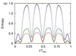
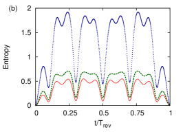
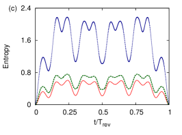
Figure 13: Entanglement measures versus $t/T_{rev}$ for initial states (a)$\ket{\psi_{00}}$, (b) $\ket{\psi_{10}}$ and (c) $\ket{\psi_{11}}$ with $\alpha_{a}=\alpha_{b}=1$. $S(A:B)$, SVNE and SLE are respectively given by the solid red curve, the blue dotted curve and the green dashed curve.

In this paper we have established how tomograms can be exploited to identify and characterize a variety of nonclassical effects such as the wave packet revival phenomena and squeezing and higher-order squeezing in both single-mode and bipartite systems. While a simple relation has been shown to exist between the number of strands in tomogram patterns and the nature of fractional revivals when a single-mode radiation field propagates in a Kerr-like medium [18] our investigations reveal that this no longer holds even in single-mode systems which display super-revivals during temporal evolution. We have also analyzed the revival phenomena in bipartite systems such as the double-well BEC evolving in time, solely from tomograms. We have obtained the extent of squeezing and also higher-order Hong-Mandel and Hillery type squeezing for both systems from tomograms. We have also investigated entropic squeezing and the extent of bipartite entanglement in detail from the tomograms alone in the case of the double-well BEC and suggested how an entanglement measure which mimics the SVNE and the SLE can be obtained from the tomograms at all instants of time. In the single-mode example we have considered initial states which are either CS or PACS and in the bipartite system the initial states are factored products of CS and states which marginally depart from macroscopic coherence.

We have also undertaken similar investigations on the Jaynes-Cummings model of field-atom interactions. This helps in identifying how tomograms of systems with a few atomic energy levels differ from those of multi-level atoms. These results will be reported elsewhere.

The primary advantage of studying experimentally obtained tomograms in detail is that the entire state-reconstruction machinery can be bypassed in examining the nature and extent of nonclassical effects. This tomographic approach becomes particularly useful when examining physical systems which are evolving in time, because state reconstruction procedures at several different instants can be avoided. We have established how a wide spectrum of nonclassical effects can be quantitatively evaluated solely from tomograms.

Appendix

Numerical computation of the two-mode density matrix

We outline the essential steps in computing the density matrix $\rho_{m_{1},m_{2}}(t)$ of the double-well BEC, for initial states $\ket{\psi_{m_{1}m_{2}}}=\ket{\alpha_{a},m_{1}}\otimes\ket{\alpha_{b},m_{2}}$ with Hamiltonian $H_{bec}$ (17).

The procedure for obtaining $\rho_{0,0}(t)$ the time-evolved density matrix corresponding to the initial state $\ket{\alpha_{a}}\otimes\ket{\alpha_{b}}$ is outlined in [26]. We obtain $\rho_{m_{1},m_{2}}(t)=\ket{\psi_{m_{1}m_{2}}(t)}\bra{\psi_{m_{1}m_{2}}(t)}$ from $\rho_{0,0}(t)$ through appropriate transformations. We first write

$$\ket{\psi_{m_{1}m_{2}}(t)}=M_{m_{1},m_{2}}(t)\ket{\psi_{00}(t)},$$ (36)

where

$$M_{m_{1},m_{2}}(t)=\frac{1}{\kappa}\exp(-\rmi H_{bec}t)a^{\dagger m_{1}}b^{\dagger m_{2}}\exp(\rmi H_{bec}t),$$ (37)

and $\kappa$ is given in terms of Laguerre polynomials as $\sqrt{m_{1}!L_{m_{1}}(-{|\alpha_{a}|}^{2})m_{2}!L_{m_{2}}(-{|\alpha_{b}|}^{2})}$. In order to recast $M_{m_{1},m_{2}}(t)$ in a simpler form we introduce the operator $V=\exp(\gamma(a^{\dagger}b-b^{\dagger}a)/2)$, where $\gamma=\cos^{-1}(\omega_{1}/\lambda_{1})$[26]. Consequently, $H_{bec}$ can be written as $VH_{V}V^{\dagger}$, where $H_{V}=\omega_{0}N_{tot}+\lambda_{1}(a^{\dagger}a-b^{\dagger}b)+U_{ab}N_{tot}^{2}$. Hence,

$$M_{m_{1},m_{2}}(t)=\frac{1}{\kappa}V\exp(-\rmi H_{V}t)V^{\dagger} a^{\dagger m_{1}}b^{\dagger m_{2}}$$ (38)

$$V\exp(\rmi H_{V}t)V^{\dagger}.$$

This expression can now be simplified using the following identities which can be obtained in a straightforward manner by using the Baker-Hausdorff lemma.

$$V^{\dagger}a^{\dagger}V=a^{\dagger}\cos(\gamma/2)+b^{\dagger}\sin(\gamma/2),$$ (39)

$$V^{\dagger}b^{\dagger}V=b^{\dagger}\cos(\gamma/2)-a^{\dagger}\sin(\gamma/2),$$ (40)

$$Va^{\dagger}V^{\dagger}=a^{\dagger}\cos(\gamma/2)-b^{\dagger}\sin(\gamma/2),$$ (41)

$$Vb^{\dagger}V^{\dagger}=b^{\dagger}\cos(\gamma/2)+a^{\dagger}\sin(\gamma/2),$$ (42)

$$\exp(-\rmi\lambda_{1}(a^{\dagger}a-b^{\dagger}b)t)a^{\dagger p}b^{\dagger q}\exp(\rmi\lambda_{1}(a^{\dagger}a-b^{\dagger}b)t)$$

$$=a^{\dagger p}b^{\dagger q}\exp(-\rmi(p-q)\lambda_{1}t),$$ (43)

$$\exp(-\rmi\omega_{0}N_{tot}t)a^{\dagger p}b^{\dagger q}\exp(\rmi\omega_{0}N_{tot}t)$$

$$=a^{\dagger p}b^{\dagger q}\exp(-\rmi(p+q)\omega_{0}t),$$ (44)

$$\exp(-\rmi U_{ab}N_{tot}^{2}t)a^{\dagger p}b^{\dagger q}\exp(\rmi U_{ab}N_{tot}^{2}t)$$

$$=a^{\dagger p}b^{\dagger q}\exp(-\rmi U_{ab}t(p+q)(2N_{tot}+p+q)).$$ (45)

Further, using binomial expansions for the two commuting operators $a^{\dagger}$ and $b^{\dagger}$ and defining $p_{max}=(k+m_{2}-l)$ and $q_{max}=(l+m_{1}-k)$, we arrive at the following simplified expression for $M_{m_{1},m_{2}}(t)$.

$$M_{m_{1},m_{2}}(t)=\frac{1}{\kappa}\biggl{[}\sum_{k=0}^{m_{1}}\sum_{l=0}^{m_{2}}\sum_{p=0}^{p_{max}}\sum_{q=0}^{q_{max}}(-1)^{k-p}{m_{1}\choose k}{m_{2}\choose l}$$

$$\hskip 20.00003pt{p_{max}\choose p}{q_{max}\choose q}\exp(-\rmi\lambda_{1}t(2(k-l)+m_{2}-m_{1}))$$

$$\hskip 20.00003pt(\cos(\gamma/2))^{(k+l+p+q)}(\sin(\gamma/2))^{(2(m_{1}+m_{2})-(k+l+p+q))}$$

$$\hskip 20.00003pta^{\dagger(p+q_{max}-q)}b^{\dagger(q+p_{max}-p)}\biggr{]}\exp(-\rmi\omega_{0}t(m_{1}+m_{2}))$$

$$\times\exp(-\rmi U_{ab}t(m_{1}+m_{2})(2N_{tot}+m_{1}+m_{2})).$$ (46)

The density matrix can now be expressed in terms of $M_{m_{1},m_{2}}(t)$ and $\rho_{0,0}(t)$ as

$$\rho_{m_{1},m_{2}}(t)=M_{m_{1},m_{2}}(t)\rho_{0,0}(t)M^{\dagger}_{m_{1},m_{2}}(t).$$ (47)

References

References

- [1] Slusher R E, Hollberg L W, Yurke B, Mertz J C and Valley J F 1985 Phys. Rev. Lett. 55(22) 2409–2412 URL http://link.aps.org/doi/10.1103/PhysRevLett.55.2409
- [2] Vahlbruch H, Chelkowski S, Hage B, Franzen A, Danzmann K and Schnabel R 2006 Phys. Rev. Lett. 97(1) 011101 URL http://link.aps.org/doi/10.1103/PhysRevLett.97.011101
- [3] Sudheesh C, Lakshmibala S and Balakrishnan V 2005 Journal of Optics B: Quantum and Semiclassical Optics 7 S728 URL http://stacks.iop.org/1464-4266/7/i=12/a=040
- [4] Sudheesh C, Lakshmibala S and Balakrishnan V 2006 Journal of Physics B: Atomic, Molecular and Optical Physics 39 3345 URL http://stacks.iop.org/0953-4075/39/i=16/a=017
- [5] Gutschick V P and Nieto M M 1980 Phys. Rev. D 22(2) 403–418 URL http://link.aps.org/doi/10.1103/PhysRevD.22.403
- [6] Robinett R 2004 Physics Reports 392 1 – 119 ISSN 0370-1573 URL http://www.sciencedirect.com/science/article/pii/S0370157303004381
- [7] Averbukh I S and Perelman N 1990 Acta Phys. Pol. A 78 33–40
- [8] Agarwal G S and Banerji J 1998 Phys. Rev. A 57(5) 3880–3884 URL http://link.aps.org/doi/10.1103/PhysRevA.57.3880
- [9] Bluhm R and Kostelecký V A 1995 Phys. Rev. A 51(6) 4767–4786 URL http://link.aps.org/doi/10.1103/PhysRevA.51.4767
- [10] Seltzer S J, Meares P J and Romalis M V 2007 Phys. Rev. A 75(5) 051407 URL http://link.aps.org/doi/10.1103/PhysRevA.75.051407
- [11] Greiner M, Mandel O, Hänsch T W and Bloch I 2002 Nature 419 51–54
- [12] Estéve J, Gross C, Weller A, Giovanazzi S and Oberthaler M K 2008 Nature 455 1216–1219
- [13] Muessel W, Strobel H, Linnemann D, Zibold T, Juliá-Díaz B and Oberthaler M K 2015 Phys. Rev. A 92(2) 023603 URL http://link.aps.org/doi/10.1103/PhysRevA.92.023603
- [14] Vogel K and Risken H 1989 Phys. Rev. A 40(5) 2847–2849 URL http://link.aps.org/doi/10.1103/PhysRevA.40.2847
- [15] Ibort A, Man’ko V I, Marmo G, Simoni A and Ventriglia F 2009 Physica Scripta 79 065013 URL http://stacks.iop.org/1402-4896/79/i=6/a=065013
- [16] Lvovsky A I and Raymer M G 2009 Rev. Mod. Phys. 81(1) 299–332 URL http://link.aps.org/doi/10.1103/RevModPhys.81.299
- [17] Barnett S M and Radmore P M 1997 Methods in theoretical quantum optics vol 15 (Clarendon Press, Oxford)
- [18] Rohith M and Sudheesh C 2015 Phys. Rev. A 92(5) 053828 URL http://link.aps.org/doi/10.1103/PhysRevA.92.053828
- [19] Rohith M and Sudheesh C 2016 J. Opt. Soc. Am. B 33 126–133 URL http://josab.osa.org/abstract.cfm?URI=josab-33-2-126
- [20] Orłowski A 1997 Phys. Rev. A 56(4) 2545–2548 URL http://link.aps.org/doi/10.1103/PhysRevA.56.2545
- [21] Zavatta A, Viciani S and Bellini M 2005 Phys. Rev. A 72(2) 023820 URL http://link.aps.org/doi/10.1103/PhysRevA.72.023820
- [22] Filippov S N and Man’ko V I 2011 Physica Scripta 83 058101 URL http://stacks.iop.org/1402-4896/83/i=5/a=058101
- [23] Tara K, Agarwal G S and Chaturvedi S 1993 Phys. Rev. A 47(6) 5024–5029 URL http://link.aps.org/doi/10.1103/PhysRevA.47.5024
- [24] Hillery M 1987 Phys. Rev. A 36(8) 3796–3802 URL http://link.aps.org/doi/10.1103/PhysRevA.36.3796
- [25] Wünsche A 1996 Phys. Rev. A 54(6) 5291–5294 URL http://link.aps.org/doi/10.1103/PhysRevA.54.5291
- [26] Sanz L, Moussa M and Furuya K 2006 Annals of Physics 321 1206 – 1220 ISSN 0003-4916 URL http://www.sciencedirect.com/science/article/pii/S0003491605001569
- [27] Kuang L M, Wang F B and Zhou Y G 1994 Journal of Modern Optics 41 1307–1318 (Preprint http://dx.doi.org/10.1080/09500349414551261) URL http://dx.doi.org/10.1080/09500349414551261
- [28] Nielsen M A and Chuang I L 2010 Quantum computation and quantum information (Cambridge University Press)