Oxygen abundance maps of CALIFA galaxies

Abstract

We construct maps of the oxygen abundance distribution across the disks of 88 galaxies using CALIFA data release 2 (DR2) spectra. The position of the center of a galaxy (coordinates on the plate) were also taken from the CALIFA DR2. The galaxy inclination, the position angle of the major axis, and the optical radius were determined from the analysis of the surface brightnesses in the SDSS $g$ and $r$ bands of the photometric maps of SDSS data release 9. We explore the global azimuthal abundance asymmetry in the disks of the CALIFA galaxies and the presence of a break in the radial oxygen abundance distribution. We found that there is no significant global azimuthal asymmetry for our sample of galaxies, i.e., the asymmetry is small, usually lower than 0.05 dex. The scatter in oxygen abundances around the abundance gradient has a comparable value, $\lesssim 0.05$ dex. A significant (possibly dominant) fraction of the asymmetry can be attributed to the uncertainties in the geometrical parameters of these galaxies. There is evidence for a flattening of the radial abundance gradient in the central part of 18 galaxies. We also estimated the geometric parameters (coordinates of the center, the galaxy inclination and the position angle of the major axis) of our galaxies from the analysis of the abundance map. The photometry-map-based and the abundance-map-based geometrical parameters are relatively close to each other for the majority of the galaxies but the discrepancy is large for a few galaxies with a flat radial abundance gradient.

1 Introduction

It has been well known for a long time that the disks of spiral galaxies show negative radial abundance gradients, in the sense that the abundance is higher at the centre and decreases with galactocentric distance (Searle, 1971; Smith, 1975). It is a common practice to describe the nebular abundance distribution across the disk of a galaxy by the relation between oxygen abundance O/H and galactocentric distance $R{{}_{g}}$ and to specify this distribution by the characteristic abundance (the abundance at a given galactocentric distance, e.g., abundance at the centre of the disk) and by the radial abundance gradient. Relations of this type were determined for many galaxies by different authors (Vila-Costas & Edmunds, 1992; Zaritsky et al., 1994; Pilyugin et al., 2006, 2007, 2014a, 2015; Moustakas et al., 2010; Gusev et al., 2012; Sánchez et al., 2014; Sánchez-Menguiano et al., 2016, among many others). Such relations are based on the assumption that the abundance distribution across the disk is axisymmetric.

The azimuthal abundance variations across the disk of a galaxy were discussed in a number of papers. The dispersion in abundance at fixed radius (the scatter around the general O/H – $R_{g}$ trend, residuals) is used as the measure of the azimuthal abundance variations (e.g. Kennicutt & Garnett, 1996; Martin & Belley, 1996; Bresolin, 2011; Li, Bresolin & Kennicutt, 2013; Berg et al., 2015; Croxall et al., 2015). The number of data points in such investigations is usually small. The two-dimensional abundance distribution was analyzed for the galaxy NGC 628 (Rosales-Ortega et al., 2011).

The observations obtained by the CALIFA survey (Calar Alto Legacy Integral Field Area survey; Sánchez et al., 2012) provide the possibility to construct abundance maps for disk galaxies. This allows one to investigate the distribution of abundances across the disk in detail, in particular the global azimuthal asymmetry of abundance in the disks of galaxies. We define the global azimuthal asymmetry in abundance in the following way. We divide the target galaxy into two semicircles and determine the difference between the arithmetic means of the residuals for the opposite semicircles. The differences are determined for the different position angles of the dividing line. The maximum absolute value of this difference is adopted as a measure of the global azimuthal asymmetry of abundance in the disk of a galaxy. In the present work, we will determine the values of the global azimuthal abundance asymmetry in the disks of the CALIFA galaxies and compare them with the level of azimuthal abundance variations.

Thus, the goal of this investigation is to construct maps of the oxygen abundance distribution in the disks of the selected CALIFA galaxies and to use those maps to explore the presence (or lack) of a global azimuthal asymmetry in the oxygen abundance as well the existence of a break in the radial oxygen abundance distribution, e.g., a flattening of the radial abundance gradient at the central part of a galaxy. Evidence for a decrease of the oxygen abundances in the central parts of a number of the CALIFA galaxies was found by Sánchez et al. (2014).

We also examine whether the geometric parameters of a galaxy (coordinates of the center, inclination and position angle of the major axis) can be estimated from the analysis of the abundance map. The geometric parameters of a galaxy are usually determined from the analysis of the photometric or/and velocity map of the galaxy under the assumption that the surface brightness of the galaxy (or the velocity field) is a function of the radius only, i.e., that there is no azimuthal asymmetry in brightness (or velocity). Since the metallicity in the disk is also a function of the galactocentric distance one may expect that the abundance map can also be used for the determination of the geometric parameters of a galaxy. We will determine the “chemical” (abundance-map-based) geometrical parameters of our galaxies and compare them to their “photometric” (canonical, photometry-map-based) geometrical parameters.

The paper is organized in the following way. The algorithm employed in our study is described in the Section 2. The results and discussion are given in Section 3. Section 4 is a brief summary.

Throughout the paper, we will use the following notations for the line fluxes: $R_{2}$ = $I_{\rm\rm[OII]\lambda 3727+\lambda 3729}/I_{\rm{\rm H}\beta}$, $N_{2}$ = $I_{\rm\rm[NII]\lambda 6548+\lambda 6584}/I_{\rm{\rm H}\beta}$, $S_{2}$ = $I_{\rm\rm[SII]\lambda 6717+\lambda 6731}/I_{\rm{\rm H}\beta}$, $R_{3}$ = $I_{\rm{\rm[OIII]}\lambda 4959+\lambda 5007}/I_{\rm{\rm H}\beta}$. The units of the wavelengths are angstroms.

2 Algorithm

2.1 The emission line fluxes

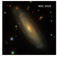
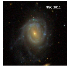
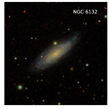
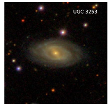
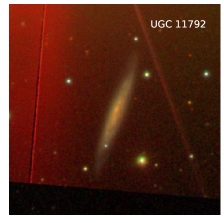
Figure 1: An example of SDSS images of CALIFA galaxies from our sample.

We used publicly available spectra from the integral field spectroscopic CALIFA survey data release 2 (DR2; Sánchez et al., 2012; García-Benito et al., 2014; Walcher et al., 2014) based on observations with the PMAS/PPAK integral field spectrophotometer mounted on the Calar Alto 3.5-meter telescope. CALIFA DR2 provides wide-field IFU data for 200 galaxies. In Fig. 1 we present an example of SDSS images of six galaxies. The data for each galaxy consist of two spectral datacubes, which cover the spectral regions of 4300–7000 Å at a spectral resolution of $R\sim 850$ (setup V500) and of 3700–5000 Å at $R\sim 1650$ (setup V1200).

The spectrum of each spaxel from the CALIFA DR2 datacubes (setup V500) is processed into two steps.

First, the stellar background in all spaxels is fitted using the public version of the STARLIGHT code (Cid Fernandes et al., 2005; Mateus et al., 2006; Asari et al., 2007). We use a set of 45 synthetic simple stellar population (SSP) spectra with metallicities $Z=0.004$, 0.02, and 0.05, and 15 ages from 1 Myr up to 13 Gyr from the evolutionary synthesis models of Bruzual & Charlot (2003) and the reddening law of Cardelli, Clayton & Mathis (1989) with $R_{V}=3.1$. The resulting stellar radiation contribution is subtracted from the measured spectrum in order to find the nebular emission spectrum. Second, the emission lines are fitted by Gaussians. The widths of the individual lines of the doublets [OIII]$\lambda$$\lambda$4959,5007, [NII]$\lambda$$\lambda$6548,6584, and [SII]$\lambda$$\lambda$6717,6731 are set to be equal to each other for each doublet. Since only the low resolution (V500 setup) spectra are used the [OII]$\lambda$$\lambda$3727,3729 doublet is fitted by a single Gaussian. Applying $\chi^{2}$ minimization, the estimation of the flux error relies on the $\chi^{2}$ quadratic approximation in the neighborhood of the $\chi^{2}$ minimum based on a Hessian matrix.

For each spectrum, we measure the fluxes of the [O ii]$\lambda$3727+$\lambda$3729, H$\beta$, [O iii]$\lambda$4959, [O iii]$\lambda$5007, [N ii]$\lambda$6548, H$\alpha$, [N ii]$\lambda$6584, [S ii]$\lambda$6717, [S ii]$\lambda$6731 lines. The measured line fluxes are corrected for interstellar reddening using the theoretical H$\alpha$ to H$\beta$ ratio (i.e., the standard value of H$\alpha$/H$\beta$ = 2.86) and the analytical approximation of the Whitford interstellar reddening law from Izotov et al. (1994). When the measured value of H$\alpha$/H$\beta$ is lower than 2.86 the reddening is adopted to be zero.

The [O iii]$\lambda$5007 and $\lambda$4959 lines originate from transitions from the same energy level, so their flux ratio is determined only by the transition probability ratio, which is very close to 3 (Storey & Zeippen, 2000). The stronger line [O iii]$\lambda$5007 is usually measured with higher precision than the weaker line [O iii]$\lambda$4959. Therefore, the value of $R_{3}$ is estimated as $R_{3}=1.33$ [O iii]$\lambda$5007 but not as a sum of the line fluxes. Similarly, the [N ii]$\lambda$6584 and $\lambda$6548 lines also originate from transitions from the same energy level and the transition probability ratio for those lines is again close to 3 (Storey & Zeippen, 2000). The value of $N_{2}$ is therefore estimated as $N_{2}=1.33$ [N ii]$\lambda$6584. Thus, the lines H$\beta$, [O iii]$\lambda$5007, H$\alpha$, [N ii]$\lambda$6584, [S ii]$\lambda$6717, and [S ii]$\lambda$6731 are used for the dereddening and the abundance determinations. The precision of the line flux is specified by the ratio of the flux to the flux error (parameter $\epsilon$). We select spectra where the parameter $\epsilon\geq 3$ for each of those lines.

2.2 Abundance determinations

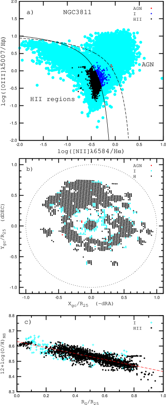
Figure 2: NGC 3811. Panel a shows the BPT diagnostic diagram (Baldwin et al., 1981). The solid and dashed curves are the boundary between AGNs and H ii regions defined by Kauffmann et al. (2003) and Kewley et al. (2001), respectively. The light-blue filled circles show the large sample of emission-line SDSS galaxies studied by Thuan et al. (2010). The red points are AGN-like objects in NGC3811 according to the dividing line of Kewley et al. (2001). The black points are H ii-region-like objects in NGC3811 according to the dividing line of Kauffmann et al. (2003). The dark-blue points are “intermediate” objects in NGC3811 located between the dividing lines of Kauffmann et al. (2003) and Kewley et al. (2001). Panel b shows the locations of the AGN-like, H ii-region-like, and “intermediate” objects in NGC3811 in the deprojected image of the galaxy. Panel c shows the radial distribution of oxygen abundances in the disk of the galaxy NGC3811 traced by the H ii-region-like (black points) and “intermediate” (cyan-colored crosses) objects.

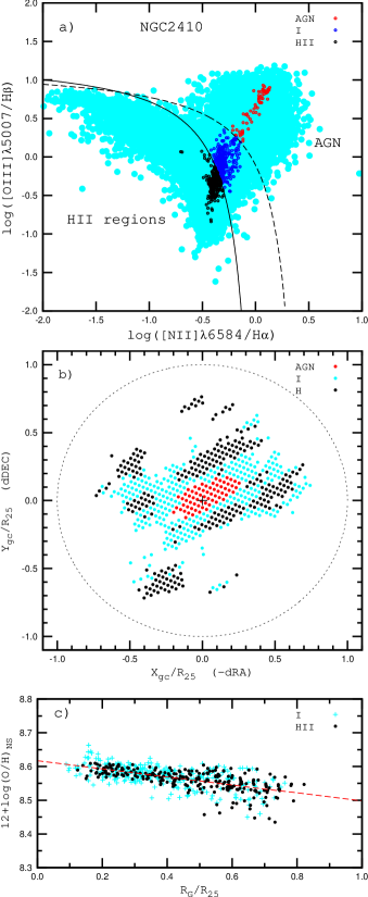
Figure 3: NGC 2410. The panels and symbols are the same as in Fig. 2.

If weak auroral lines such as such as [O iii]$\lambda$4363 are detected in the spectrum of an H ii region the oxygen abundance can be derived using the direct $T_{e}$ method, which is considered to yield the most reliable nebular oxygen abundance determinations (e.g., Dinerstein, 1990). This method requires the measurement of reddening-corrected diagnostic line ratios and knowledge of the local physical conditions (i.e., the effective tempeature of the gas, $T_{e}$, and its electron density). $T_{e}$ is then usually determined from the intensity ratio of the auroral to nebular lines of doubly ionized oxygen; in other words, directly from the observed line ratios (hence the name “direct $T_{e}$ method”). A short description of the required steps is given in Dinerstein (1990). More details can be found in Aller (1984) and Osterbrock (1989).

In our current study, the oxygen abundances will be determined through a strong-line method (the $C$ method (Pilyugin et al., 2012, 2013)) since the auroral lines are undetectable in the majority of the CALIFA spectra (Marino et al., 2013) and, consequently, the $T_{e}$ method cannot be applied. The $C$ method is based on the assumption that H ii regions with a similar combination of intensities of metallicity-sensitive strong emission lines have similar abundances. When the strong lines [O iii]$\lambda$4959,5007, [N ii]$\lambda$6548,6584, and [S ii]$\lambda$6717,6731 are measured in the spectrum of an H ii region the oxygen (O/H)${}_{C_{\rm NS}}$ abundance can be determined. When the strong lines [O ii]$\lambda$3727,3729, [O iii]$\lambda$4959,5007, and [N ii]$\lambda$6548,6584 are measured in the spectrum then we can determine the oxygen (O/H)${}_{C_{\rm ON}}$ abundance.

Since the oxygen line [O ii]$\lambda$3727+$\lambda$3729 is not available or noisy in many spectra of the CALIFA-V500 setup the $C_{NS}$ variant of the $C$ method is used for the abundance determination in the H ii regions. It should be emphasized that our analysis is restricted to the V500 setup data.

In order to improve the accuracy of the $C$ method we have updated our sample of reference H ii regions that are used for the abundance determination with this method. New spectral measurements of H ii regions with detected auroral lines were added to our collection (Berg et al., 2012; Izotov, Thuan & Guseva, 2012; Zurita & Bresolin, 2012; Berg et al., 2013; Haurberg, Rosenberg & Salzer, 2013; Li, Bresolin & Kennicutt, 2013; Skillman et al., 2013; Brown, Croxall & Pogge, 2014; Esteban et al., 2014; Nicholls et al., 2014; Annibali et al., 2015; Berg et al., 2015; Croxall et al., 2015; Haurberg et al., 2015). The abundances in those H ii regions were determined through the $T_{e}$ method. The realization of the $T_{e}$ method, i.e., the equations of the $T_{e}$ method that serve to convert the values of the line fluxes to electron temperatures and abundances, are described in numerous papers (e.g., Pagel et al., 1992; Izotov et al., 2006; Pilyugin et al., 2010). The equations adopted in our current study were derived from the five-level atom solution with recent atomic data (Einstein coefficients for spontaneous transitions, energy level data, and effective cross sections for electron impact) in Pilyugin et al. (2010). Using the collected data with $T_{e}$-based abundances we select a sample of reference H ii regions following Pilyugin et al. (2013), i.e., we select a sample of reference H ii regions for which the absolute differences of the oxygen abundances (O/H)${}_{C_{\rm ON}}$ – (O/H)${}_{T_{e}}$ and (O/H)${}_{C_{\rm NS}}$ – (O/H)${}_{T_{e}}$ and of the nitrogen abundances (N/H)${}_{C_{\rm ON}}$ – (N/H)${}_{T_{e}}$ and (N/H)${}_{C_{\rm NS}}$ – (N/H)${}_{T_{e}}$ are less than 0.1 dex. This sample of reference H ii regions contains 313 objects and will be used for the abundance determinations in the present paper. This sample of H ii regions has been also used as calibration data in the construction of a new calibration for abundance determinations in H ii regions (Pilyugin & Grebel, 2016). The good agreement between the calibration-based and $T_{e}$-based abundances suggests that our reference sample does indeed contain H ii regions with reliable oxygen abundances (O/H)${}_{T_{e}}$. We determine the oxygen abundance in the target object by comparing it with 30 counterpart reference H ii regions in order to decrease the influence of the uncertainties in the oxygen abundances of the individual reference H ii regions on the resulting abundance of the target objects.

Since the abundances produced by the $C$ method and $T_{e}$ method are close to each other our approach is very similar to using the empirical metallicity scale defined by H ii regions with oxygen abundances derived through the direct method ($T_{e}$ method). This conclusion has been confirmed in our recent studies (Pilyugin et al., 2015; Zinchenko et al., 2015). It has been well known for a long time that the oxygen abundances produced by the calibrations based on H ii regions with $T_{e}$-based measurements and calibrations based on photoionization models can differ by up to 0.7 dex (e.g., Pilyugin et al., 2001, 2003b; Kewley & Ellison, 2008; Moustakas et al., 2010; López-Sánchez & Esteban, 2010; Bresolin et al., 2009, 2012).

There are different types of objects with emission-line spectra, e.g., H ii region-like objects, AGN-like objects, and LINER-like objects. The intensities of the strong lines can be used to separate different types of emission-line objects according to their main excitation mechanism. Baldwin et al. (1981) proposed a diagnostic diagram (the so-called BPT classification diagram) where the excitation properties of H ii regions are established from the [N ii]$\lambda$6584/H$\alpha$ and [O iii]$\lambda$5007/H$\beta$ line ratios. The location of the different classes of the emission-line objects in the [N ii]$\lambda$6584/H$\alpha$ and [O iii]$\lambda$5007/H$\beta$ and other diagrams were investigated in many studies (e.g., Kewley et al., 2001; Kauffmann et al., 2003; Stasińska et al., 2006; Singh et al., 2013; Vogt et al., 2014; Belfiore et al., 2015; Sánchez et al., 2015b). The exact location of the dividing line between H ii regions and AGNs is still under debate.

The demarcation line of Kauffmann et al. (2003) in the [N ii]$\lambda$6584/H$\alpha$ vs. [O iii]$\lambda$5007/H$\beta$ diagram seems to be the most stringent condition to select true H ii regions (Vogt et al., 2014). However, an appreciable fraction of H ii regions is located to the right (thus on the “wrong” side) of this demarcation line (Sánchez et al., 2015b). The goal of the current study is to construct metallicity maps of galaxies. Thus we are interested in using as many points as possible. Some H ii regions are lost when the demarcation line of Kauffmann et al. (2003) is adopted. Can one avoid the loss of data points with reliable $C$-based abundances?

Panel $a$ of Fig. 2 shows the [N ii]$\lambda$6584/H$\alpha$ vs. [O iii]$\lambda$5007/H$\beta$ diagram for the spectra of individual spaxels in the galaxy NGC 3811. Solid and dashed curves mark the boundary between AGNs and H ii regions defined by Kauffmann et al. (2003) and Kewley et al. (2001), respectively. The light-blue filled circles show the large sample of emission-line SDSS galaxies studied by Thuan et al. (2010). The red points indicate AGN-like objects in NGC3811 according to the dividing line of Kewley et al. (2001). The black points represent H ii-region-like objects in NGC3811 according to the dividing line of Kauffmann et al. (2003). The dark-blue points are “intermediate” objects in NGC 3811 located between the dividing lines of Kauffmann et al. (2003) and Kewley et al. (2001). Panel $b$ shows the locations of the AGN-like, H ii-region-like, and “intermediate” objects in NGC 3811 in the deprojected face-on image of the galaxy. Panel $c$ shows the radial distribution of oxygen abundances in the disk of the galaxy NGC 3811 traced by the H ii-region-like and “intermediate” objects. Fig. 3 shows similar diagrams for NGC 2410. The BPT diagram for NGC 2410 differs from that for NGC 3811. There is a well-defined AGN branch in the case of NGC 2410. Panels $c$ in Fig. 2 and Fig. 3 clearly show that the abundances of the intermediate objects closely follow the general radial oxygen abundance trends traced by the H ii regions selected with the dividing line of Kauffmann et al. (2003). Therefore the demarcation line of Kewley et al. (2001) is adopted here.

It should be emphasized that we do not claim to establish the exact locus of the boundary between the H ii region-like and other classes of emission line objects. We only illustrate that the $C$-based abundances in the objects located left of (or below) the demarcation line of Kauffmann et al. (2003) and the objects located between the demarcation lines of Kauffmann et al. (2003) and Kewley et al. (2001) show the same radial oxygen abundance trend in the disks of our target galaxies.

2.3 The radial abundance gradient

The galaxy inclination and position angle of the major axis are estimated from the analysis of the surface brightness map in the $r$ band of the Sloan Digital Sky Survey (SDSS). We constructed radial surface brightness profiles in the SDSS $g$ and $r$ bands using the photometric maps of SDSS data release 9 (Ahn et al., 2012) in the same way as in Pilyugin et al. (2014b). The optical isophotal radius $R_{25}$ of a galaxy is determined from the analysis of the surface brightness profiles in the SDSS $g$ and $r$ bands converted to the Vega $B$ band. We use the spaxel coordinates of the CALIFA plates. The location of the center of the galaxy is at $X_{0}$ and $Y_{0}$. The galactocentric $X$-coordinate is the right ascension offset with opposite sign. The galactocentric $Y$-coordinate is the declination offset. Since the size of a spaxel is equal to one arcsec the offset in spaxels is equal to the offset in arcsec. We also use fractional radii, i.e., radii normalized to the optical isophotal radius $R_{25}$.

The radial oxygen abundance distribution within the optical isophotal radius of the disk, $R_{25}$, is fitted by the following expression, which will be referred to as the O/H – $R_{G}$ relation:

$$12+\log({\rm O/H})=12+\log({\rm O/H})_{0}+grad\times(R/R_{25}),$$ (1)

where 12 + log(O/H)₀ is the oxygen abundance at $R_{0}=0$, i.e., the extrapolated central oxygen abundance, $grad$ is the slope of the oxygen abundance gradient expressed in terms of dex $R_{\rm 25}^{-1}$, and $R$/$R_{\rm 25}$ is the fractional radius (the galactocentric distance normalized to the disk’s isophotal radius $R_{25}$). If there is an abundance depletion in the central part of the disk then this part is excluded from the gradient estimation (for more details see Section 3.4).

The radial abundance gradient obtained using the geometrical parameters of a galaxy from an analysis of the surface brightness map will be referred as case $A$. The radial abundance gradient obtained using the geometrical parameters based on an analysis of the abundance map will be referred as case $C$ (see below).

2.4 The azimuthal asymmetry

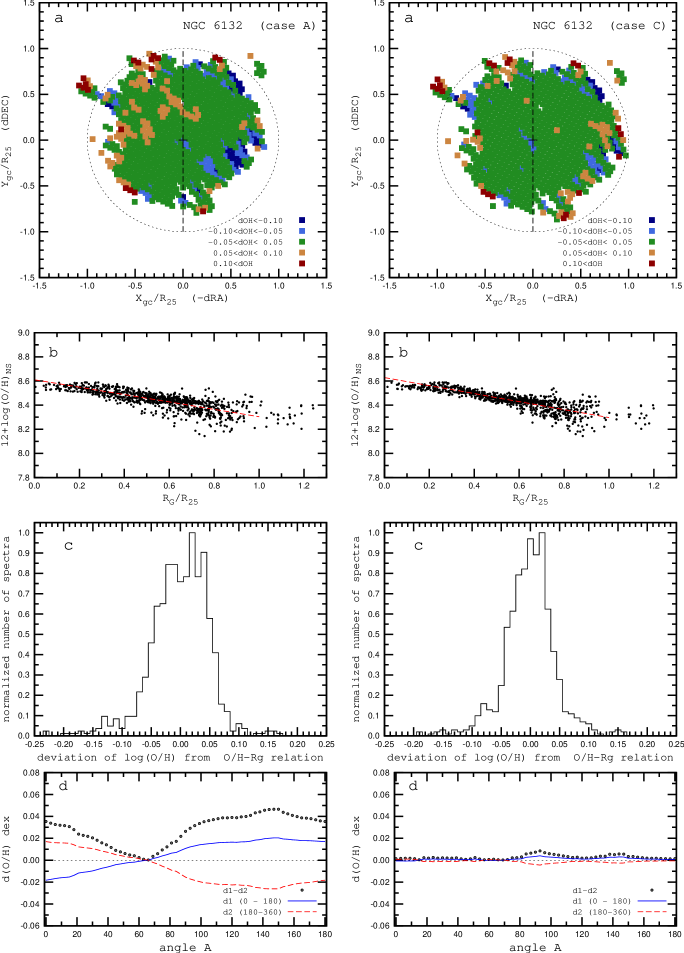
Figure 4: NGC 6132. The panels show the properties of the abundance distribution in the disk of the galaxy determined with deprojected galactocentric distances of the spaxels for the geometrical parameters of the galaxy obtained from the analysis of the photometric map (left column panels, case $A$) and with deprojected galactocentric distances of the spaxels for the geometrical parameters of the galaxy obtained from the analysis of the abundance map (right column panels, case $C$). Panel a in each column shows the locations of the spaxels with different abundance deviations from the O/H – $R_{g}$ relation in the deprojected image of the galaxy. The dark-blue squares are spaxels with d(O/H) $\leq-0.10$ dex, the light-blue squares stand for spaxels with $-0.10<$ d(O/H) $\leq-0.05$ dex, the green squares indicate spaxels with $-0.05<$ d(O/H) $\leq 0.05$ dex, the light-brown squares represent spaxels with $0.05<$ d(O/H) $\leq 0.10$ dex, and the dark-brown squares indicate spaxels with $0.10<$ d(O/H). The dashed circle marks the isophotal radius $R_{25}$, and the cross marks the center of the galaxy. Panel b shows the radial distribution of oxygen abundances in the disk of the target galaxy. The black points indicate the abundances of individual spaxels, and the red-dashed line is the linear best fit to those data points. Panel c shows the normalized histogram of oxygen abundance deviations from the O/H – $R_{g}$ relation. Panel d shows the arithmetic means of the deviations from the O/H $-R_{g}$ relation for the spaxels within the sector with azimuthal angles from $A$ to $A+180$ (blue curve) and from $A+180$ to $A+360$ (red curve), and the absolute value of difference between those means (points) as a function of angle $A$. The dashed line in panel $a$ shows the dividing line for $A=0$. The figures for other galaxies from our sample are available online.

We examine the global azimuthal asymmetry in the oxygen abundance distribution across the disk of a galaxy. We divide the galaxy into two semicircles by a dividing line at a position angle $A$. For a fixed value of the angle $A$, we determine the arithmetic mean of the deviations $d(O/H)_{1}$ from the O/H $-R_{G}$ relation for spaxels with azimuthal angles from $A$ to $A+180$ and the mean deviation $d(O/H)_{2}$ for spaxels with azimuthal angles from $A+180$ to $A+360$. The absolute value of the difference $d(O/H)=d(O/H)_{1}-d(O/H)_{2}$ is determined for different positions of $A$. The position of $A$ is counted counterclockwise from the $Y$-axis (dashed line in panel $a$ of Fig. 4) and is changed with a step size of 3$\degr$ in the computations in both the $A$ and the $C$ cases. The maximum absolute value of the difference $d(O/H)$ is used to specify the global azimuthal asymmetry in the abundance distribution across the galaxy. The position angle of the dividing line marking the maximum absolute value of the difference $d(O/H)$ will be referred to as the azimuthal asymmetry angle.

2.5 The determination of the geometric parameters of a galaxy from the analysis of the abundance map

Accurate geometric parameters of a galaxy (position of the center of a galaxy, inclination angle, and the position angle of the major axis) should be available for the determination of a reliable galactocentric distance of an H ii region (spaxel). In the present study, the position of the center of the galaxy is described by the coordinates $X_{0}$ and $Y_{0}$ of the center of the galaxy in the CCD images. It is a canonical way to determine the geometric parameters of a galaxy from the analysis of the photometric or/and velocity map of the galaxy. It is assumed that the surface brightness distribution (or velocity field) is axisymmetric. Since the metallicity in the disk is a function of the galactocentric distance one can expect that the abundance map can also be used for the determination of the geometric parameters of a galaxy. Here we examine whether the geometric parameters of a galaxy can be estimated from the analysis of the abundance map.

Hence, in addition we obtain the geometric parameters of our galaxies from the analysis of the abundance map. We search for a set of four parameters: the position of the galaxy center on the CALIFA plate (the $X_{0}$ and $Y_{0}$ coordinates in spaxels), the inclination $i$ of the galaxy, and the position angle $PA$ of the major axis. We determine those parameters from the requirement that the correlation coefficient between oxygen abundance and galactocentric distance is maximum or the scatter around O/H – $R_{g}$ relation is minimum. It should be emphasized that both conditions result in the same values of the geometrical parameters. We use the data points within the optical radius of the galaxy. If there is a flattening of the metallicity distribution in the central part of the galaxy then this area is excluded from the analysis. The optical radius of a galaxy $R_{25}$ is fixed and comes from the analysis of the photometric map.

Fig. 4 illustrates the application of the described algorithm. The galaxy NGC 6132 is a spiral Sab galaxy (morphological type $T=2.0$) at a distance of 76.5 Mpc (leda,ned). Our analysis of the $r$-band SDSS map results in an inclination angle $i=68\degr$ with a position angle of the major axis of $PA=125\degr$. The angular optical radius of the galaxy is 0.56 arcmin. This results in a linear optical radius $R_{25}=12.46$ kpc for the adopted distance. The left-column panels of Fig. 4 show the properties of the abundance distribution across the disk of NGC 6132 where the deprojected radii of the H ii regions (spaxels) were computed using the geometric parameters of the galaxy obtained from the photometric map, case $A$. From the analysis of the abundance map, we obtained the position of the “chemical center” of the galaxy at $X_{0}=34.3$ spaxels, $Y_{0}=34.3$ spaxels, a position angle of the major axis of $PA=126\degr$, and an inclination angle $i=69\degr$. The panels in the right column of Fig. 4 show the properties of the abundance distribution across the disk of NGC 6132 where the deprojected radii of the H ii regions were computed using the geometric parameters of case $C$. The abundance-map-based geometrical parameters will be estimated for each CALIFA galaxy of our sample below. The comparison between the photometry-map-based and abundance-map-based geometrical parameters can tell us something about the credibility of the abundance-map-based geometrical parameters of galaxies.

3 Results

3.1 Our sample

We consider late-type galaxies from the CALIFA DR2 list. We include in our sample galaxies with morphological type Sa and later types for which the following conditions are fulfilled: a) the number of spaxels with measured H$\beta$, [O iii]$\lambda$5007, H$\alpha$, [N ii]$\lambda$6584, [S ii]$\lambda$6717, and [S ii]$\lambda$6731 emission lines is larger than a few hundreds; b) those spaxels are distributed along the radius and with the azimuthal angle in such way that the radial abundance trend and azimuthal variations in the oxygen abundances can be investigated. The number of the data points is usually larger than three hundred for each of the selected galaxies, but we also included three galaxies with 213, 299, and 176 data points, respectively. Of course, the procedure of including/rejecting galaxies in our sample is somewhat arbitrary.

The $C$-based abundances in some galaxies (e.g., UGC 312, UGC 7012) show unusually large scatter. The difference between maximum and minimum oxygen abundances at a given galactocentric distance can be as large as up to an order of magnitude. This prevents a reliable determination of the radial abundance trend and the azimuthal variations in oxygen abundances. When we consider only the spaxels where the flux to the flux error $\epsilon>5$ for each line (instead of $\epsilon>3$) then the scatter significantly decreases. This suggests that the large scatter in the oxygen abundances in those galaxies seems to be artificial and can be attributed to the uncertainty in the flux measurements or/and to the uncertainty in the oxygen abundance determinations through the $C$ method. Those galaxies (eight galaxies) were excluded from further consideration. We also excluded three galaxies (NGC 825, NGC 2906, and UGC 3995) with very flat ($\ga-0.05$ dex) radial abundance gradients where we cannot estimate the geometrical parameters of the galaxy from the abundance map. Our final sample contains 88 CALIFA galaxies.

Table 1 lists the general characteristics of each galaxy: morphological type, isophotal radius $R_{25}$, and distance. Table 2 lists the obtained properties of the oxygen abundance distributions in the disks of our sample of CALIFA galaxies for both the photometric and abundance-map derived geometric parameters.

Figure 5 summarizes the properties of our sample of CALIFA galaxies. Figure 5 shows histograms of the distances (panel $a$), optical radii $R_{25}$ (panel $b$), morphological $T$ types (panel $c$), and central oxygen abundances 12 + log(O/H)₀ (panel $d$) for our galaxy sample. The optical radii of our galaxies range from $\sim 5$ kpc to $\sim 25$ kpc, but galaxies with radii between 10 and 16 kpc occur most frequently. The central oxygen abundances of most of the galaxies have a value between 12 + log(O/H)${}_{0}=8.5$ and 12 + log(O/H)${}_{0}=8.7$.

Figure 5: Histograms of distances (panel $a$), optical radii $R_{25}$ (panel $b$), morphological $T$ types (panel $c$), and central oxygen abundances 12 + log(O/H)₀ (panel $d$) for our sample of galaxies.

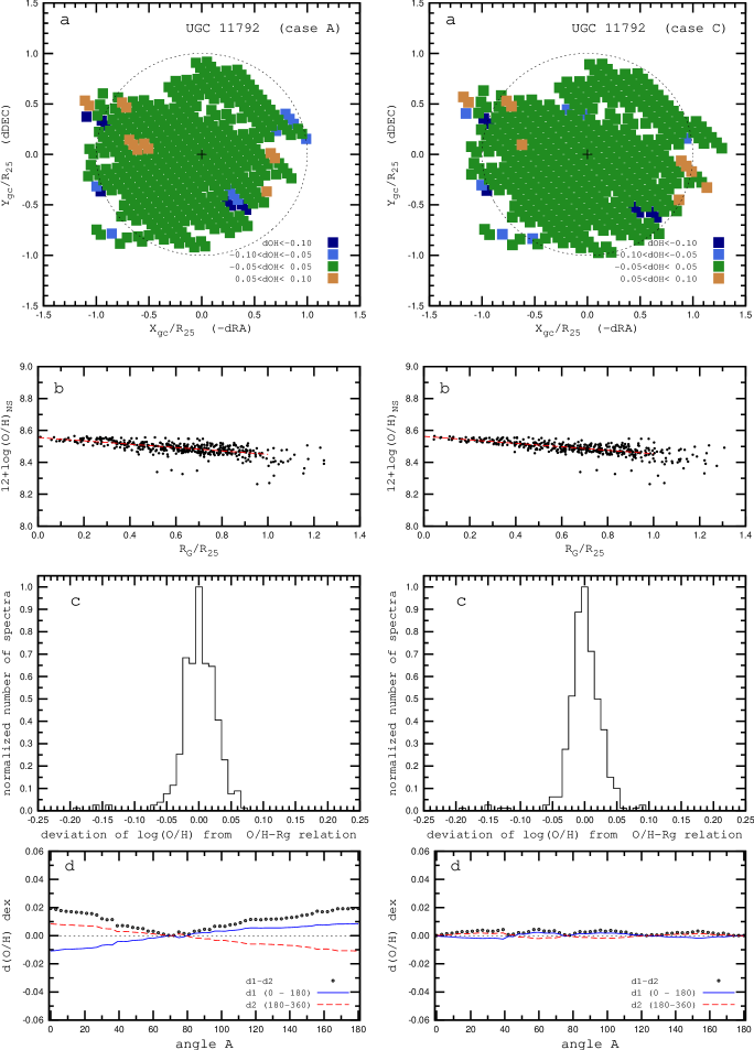
Figure 6: The galaxy UGC 11792 is a galaxy with high inclination, $i=77\degr$. The panels and symbols are the same as in Fig. 4.

A number of galaxies of our sample have a large inclination angle, $i\ga 70\degr$. Can one obtain a reliable deprojected abundance map for such galaxies? A satisfactory agreement between the photometry-map-based values and abundance-map-based geometrical parameters of such galaxies (as well as between the values of the radial abundance gradients obtained with photometry-map-based and abundance-map-based geometrical parameters; Table 2) can be considered as evidence in favor that reliable deprojected abundance maps can be obtained from the CALIFA measurements even for galaxies with an inclination up to about $80\degr$. Figure 6 shows the results for the galaxy UGC 11792 which is an example of a galaxy with high inclination, $i=77\degr$.

3.2 Comparison of the abundance-based and photometric-based geometrical parameters

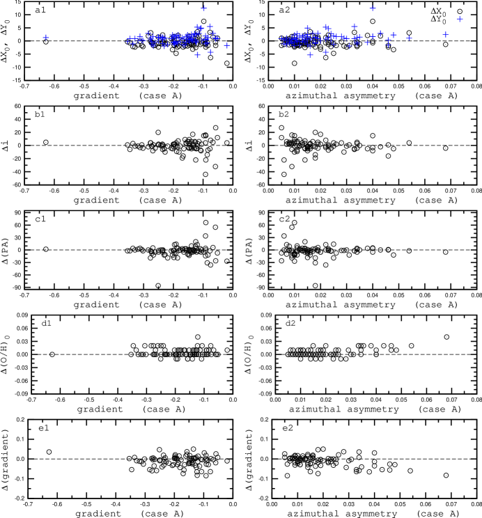
Figure 7: The difference between the geometric parameters of a galaxy (position of the center of a galaxy $X_{0}$, $Y_{0}$ (panels $a1,a2$), the inclination angle $i$ (panels $b1,b2$), and the position angle of the major axis $PA$ (panels $c1,c2$)) determined from the analysis of the abundance map and photometric map of the galaxy. The difference is plotted as a function of the radial oxygen abundance gradient across the disk (left column panels) and azimuthal asymmetry of the oxygen abundances (right column panels). The photometry-map-based radial oxygen abundance gradient and azimuthal asymmetry value (case $A$ in the text and in the previous figures) are plotted along the $X$-axis. Panels $d1$ and $d2$ show the difference between central oxygen abundances of the disk obtained with abundance-map-based and photometry-map-based geometrical parameters of a galaxy as a function of the radial abundance gradient (panel $d1$) and azimuthal asymmetry (panel $d2$). Panels $e1$ and $e2$ show the difference between radial oxygen abundance gradients across the disk obtained with abundance-map-based and photometry-map-based geometrical parameters of a galaxy as a function of the radial abundance gradient (panel $e1$) and azimuthal asymmetry (panel $e2$).

Panel $a1$ of Fig. 7 shows the differences between the coordinates of the center obtained from the analysis of the photometric maps and the coordinates obtained from the analysis of the abundance maps (the differences in the $X_{0}$ coordinates are presented by circles and the difference in the $Y_{0}$ coordinates by the plus signs) as a function of the radial abundance gradient across the optical disk of a galaxy. Panel $a2$ of Fig. 7 shows the differences between the coordinates of the center as a function of the azimuthal asymmetry in the abundance within the optical disk of a galaxy. The photometry-map-based radial abundance gradient and asymmetry value are plotted along the $X$-axis. Inspection of Fig. 7 and Table 2 show that the photometry-map-based and abundance-map-based coordinates of the centers of galaxies usually agree within 2 – 3 spaxels, i.e., the inferred photometric and chemical centers of a galaxy are usually close to each other. However, there is a large (more than 5 spaxels) disagreement between the photometry-map-based and the abundance-map-based coordinates of the centers for some galaxies with flat radial abundance gradients.

Panels $b1$ and $b2$ of Fig. 7 show the comparison between the inclination angle $i_{A}$ obtained from the analysis of the photometric maps and the inclination angle $i_{C}$ obtained from the analysis of the abundance maps. Panels $c1$ and $c2$ of Fig. 7 show the comparison between the position angle of the major axis $PA_{A}$ obtained from the analysis of the photometric maps and the position angle of the major axis $PA_{C}$ obtained from the analysis of the abundance maps. Inspection of Fig. 7 shows that the inclination angles and the position angle of the major axis derived from the analysis of the abundance maps are rather close to those obtained from the analysis of the photometric maps for the majority of our galaxies. Again, there is a large (more than 10°) disagreement between the photometry-map-based and the abundance-map-based inclination angles for some galaxies with flat radial abundance gradients. A flat radial abundance gradient (i.e., small variations of the abundance with radius) makes the accurate determination of the geometrical parameters of a galaxy from the analysis of the abundance map difficult.

The galaxy NGC 171, which has a relatively steep radial abundance gradient, $-0.25$ dex $R_{25}^{-1}$, also shows a large disagreement between the photometry-map-based and the abundance-map-based values of the inclination angle $i_{A}-i_{C}$ (panel $b1$ of Fig. 7) and between the values of the position angle of the major axis $PA_{A}-PA_{C}$ (panel $c1$ of Fig. 7). The inclination angle of the galaxy NGC 171 is small; $i_{A}=20\degr$. Therefore, the determined radial abundance gradient is not very sensitive to the values of (and error in) the values of the inclination angle and the position angle of the major axis. Hence, both the photometry-map-based and the abundance-map-based values of the inclination angle and of the position angle of the major axis can be rather uncertain.

Panels $d1$ and $d2$ show the difference between the central oxygen abundances of the disk 12+log(O/H)₀ obtained with photometry-map-based and abundance-map-based geometrical parameters of a galaxy as a function of the radial abundance gradient (panel $d1$) and asymmetry parameter (panel $d2$). The difference in the central oxygen abundance is usually small, less than 0.02 dex. Panels $e1$ and $e2$ show the difference between radial abundance gradients across the disk obtained with photometry-map-based and abundance-map-based geometrical parameters of a galaxy as a function of the radial abundance gradient (panel $e1$) and asymmetry parameter (panel $e2$). The difference is small (less than 0.05 dex $R_{25}^{-1}$) but for some galaxies it can be up to 0.1 dex $R_{25}^{-1}$.

Thus, the geometrical parameters of a galaxy can be estimated from the analysis of the abundance map.

3.3 Azimuthal asymmetry of the abundances in the disk

Figure 8: Panel $a$ shows the value (dex) of azimuthal asymmetry in the oxygen abundances in the disk of a galaxy as a function of the scatter (dex) in oxygen abundances around the O/H $-R_{g}$ relation for our sample of galaxies for case $A$ (with geometric parameters of a galaxy determined from the analysis of the photometric map). Panel $b$ shows the comparison between the values of the scatter for case $A$ and case $C$ (with geometric parameters of a galaxy determined from the analysis of the abundance map). Panel $c$ shows the comparison between the values of the azimuthal asymmetry for case $A$ and $C$. Panel $d$ shows the value of azimuthal asymmetry as a function of the scatter for case $C$.

Fig. 4 shows the galaxy NGC 6132, which is a galaxy with possible azimuthal asymmetry in the oxygen abundance in the disk. Indeed, the upper left panel of Fig. 4 shows that the points with positive oxygen abundance deviations (brown points) from the general radial abundance trend are usually located in the opposite semicircle than the points with negative oxygen abundance deviations (blue points). The difference between the means of the residuals in two semicircles divided by the line with an angle $A$ = 147$\degr$ is $\sim$0.046 dex. The scatter $\sigma$ in oxygen abundances around the O/H – $R_{g}$ relation is 0.051 dex.

Let us clarify how significant this value of azimuthal asymmetry is. Panel $a$ of Fig. 8 shows the value of azimuthal asymmetry in the oxygen abundance in the disk of a galaxy as a function of the scatter $\sigma$ in oxygen abundances around the O/H $-R_{g}$ relation for our sample of galaxies for the case $A$. The values of the global azimuthal asymmetry are small and exceed 0.04 dex for a few galaxies only.

Inspection of panel $a$ of Fig. 8 shows that there is a correlation between the value of azimuthal asymmetry and the value of the azimuthal variation (scatter $\sigma$ around of the O/H $-R_{g}$ trend) in oxygen abundance for the case $A$. On the one hand, this correlation may suggest that the azimuthal asymmetry makes a significant contribution to the scatter around the O/H – $R_{g}$ relation. This is the case if the global azimuthal asymmetry is real. On the other hand, the obtained azimuthal asymmetry may be artificial and can be caused by the uncertainties in the geometrical parameters of a galaxy or/and by the azimuthal asymmetry of the error in oxygen abundance. Since the geometric parameters for case $C$ are derived by minimizing the scatter around the O/H $-R_{g}$ relation while the geometric parameters for case $A$ are derived from the analysis of the photometric maps, the comparison of the azimuthal asymmetry and scatter for case $A$ and case $C$ allows us to check whether the obtained value of the azimuthal asymmetry for case $A$ is real.

The values of the scatter $\sigma$ in oxygen abundances around the O/H $-R_{g}$ relation for case $A$ are close to the ones for case $C$ (panel $b$ of Fig. 8). In contrast, the values of azimuthal asymmetry in the oxygen abundance for case $C$ are significantly lower than those for case $A$ (panel $c$ of Fig. 8). The values of the global azimuthal asymmetry are significantly smaller than the values of the scatter $\sigma$ in oxygen abundances around the O/H $-R_{g}$ relation for case $C$ (panel $d$ of Fig. 8). Thus, the panels $b$, $c$, and $d$ of Fig. 8 suggest that the scatter $\sigma$ in oxygen abundances around the O/H $-R_{g}$ relation cannot be attributed to the global azimuthal asymmetry in the oxygen abundance distribution. The azimuthal asymmetry obtained for case $A$ (with photometry-map-based geometrical parameters) seems to be artificial and may be caused by the uncertainties in the geometrical parameters of a galaxy at least in some galaxies.

Figure 9: Simulation of the azimuthal asymmetry parameters. Models with abundance gradient values of $-0.15$ and $-0.3$ dex $R_{\rm 25}^{-1}$ and four values of the scatter in the oxygen abundances, 0.02, 0.03, 0.04, and 0.05 dex, were considered. A random deviation of the position of the galaxy center, inclination, and the position of the major axis was introduced to simulate the uncertainties in the geometrical parameters. The panels and symbols are the same as in Fig. 8.

To verify whether the values of the global azimuthal asymmetry for the case $A$ can be caused by uncertainties in the geometrical parameters of a galaxy obtained from the analysis of the photometric map, the following numerical experiment was performed. A disk model including 400 points randomly distributed across the disk was constructed. The oxygen abundance in each point was determined from the adopted radial abundance gradient. Then the random error was added to the oxygen abundance in each point in a such way that the random abundance errors follow a Gaussian with an adopted scatter $\sigma$. Two values of the abundance gradient, $-0.15$ and $-0.3$ dex $R_{\rm 25}^{-1}$, and four values of the scatter in oxygen abundances, $\sigma$ = 0.02, 0.03, 0.04, 0.05 dex, were considered. Thus, eight disk models were examined. We considered three values of the initial inclination of a galaxy, $i=25,45$, and $65\degr$. The initial position angle of the major axis of the galaxy was fixed at $PA=45\degr$. These models do not assume any cause of the appearance of global azimuthal asymmetry, except randomly distributed errors in the oxygen abundances caused by the finite number of points in the abundance map (discussed below). Formally we can consider this case as the case $C$.

We introduced a random deviation of the position of the galaxy center $\Delta X_{0}$ and $\Delta Y_{0}$, the galaxy inclination $\Delta i$, and the position of the major axis $\Delta(PA)$. The maximal values of those deviations were chosen to be $\Delta X_{0},\Delta Y_{0}=\pm 5$ spaxels, $\Delta i=\pm 15\degr$, and $\Delta(PA)=\pm 20\degr$. Those deviations cover the range of the discrepancy between geometrical parameters in the cases $A$ and $C$ for the bulk of galaxies from our sample (see Fig. 7). Models with non-zero deviations of the geometric parameters can be regarded as the case $A$. The azimuthal asymmetry parameters were calculated for a set of 160 models. Fig. 9 shows the results of our simulations. The panels and symbols in Fig. 9 are the same as in Fig. 8. The discontinuity of the distribution of scatter is attributed to the low number of the initial values of the scatter; only four initial values of scatter in the oxygen abundances were considered. The panels $a$ and $d$ of Fig. 9, where the lowest asymmetries of case $A$ for a given scatter value are in close agreement with the asymmetries of the case $C$, confirm that minimizing the scatter in oxygen abundance and deviations of the geometric parameters results in minimizing the azimuthal asymmetry. Comparison between Fig. 8 and Fig. 9 shows clearly that our simulation reproduces the general behavior of the scatter and global azimuthal asymmetry obtained for our sample of the CALIFA galaxies. It can be considered as evidence favouring that the values of the global azimuthal asymmetry for the case $A$ can be caused by the rather small uncertainties in the geometrical parameters of a galaxy obtained from the analysis of the photometric map. The obtained range of the global azimuthal asymmetry for case $C$ can be attributed to the azimuthal asymmetry in the randomly distributed errors in the oxygen abundances.

Figure 10: The value of the global azimuthal asymmetry (left panel) and its azimuthal angle (right panel) for the case $A$ as a function of the shift of the position of the coordinates of the centre ($X_{O}$, $Y_{O}$) of the galaxies NGC 5520 (solid lines) and NGC 6132 (dashed lines) along the $X$ (circles) or $Y$ (plus signs) axes.

Figure 11: The value of the global azimuthal asymmetry as a function of the number of the spaxels in the map. The set of the abundance maps is constructed on the base of the map of the galaxy NGC 5520 by the random selection of the spaxels (see text).

To illustrate how uncertainties in the position of the galactic center affected to the global azimuthal asymmetry we consider NGC 5520 and NGC 6132. We shift the position of the galaxy’s center along the $X$ or $Y$ axis (while other geometrical parameters are fixed) and determine the value of the global azimuthal asymmetry and its azimuthal angle. The left panel of Fig. 10 shows the value of the global azimuthal asymmetry as a function of shift along the $X$ or $Y$ axis. This figure demonstrates that the range of the values of the global azimuthal asymmetry obtained for case $A$ can be reproduced by the uncertainties in the geometrical parameters of the galaxies. The right panel of Fig. 10 shows the azimuthal angle of the global azimuthal asymmetry as a function of the shift along the $X$ or $Y$ axis. This figure shows that in case of a small global azimuthal asymmetry, small uncertainties in the position of the galactic center can lead to large uncertainties in the angle of the global azimuthal asymmetry.

Azimuthal variations of the oxygen abundance across galactic disks were discussed in the literature for several galaxies. The scatter in oxygen abundance at a given radius was usually attributed to azimuthal variations in the oxygen abundance distribution. Kennicutt & Garnett (1996) have considered the dispersion in abundance at fixed radius in the disk of the galaxy M101 using 41 H ii regions. They found that there is evidence in favor of a non-axisymmetric abundance distribution. However, they noted that more data are needed to test whether this asymmetry is real. Li, Bresolin & Kennicutt (2013) obtained and analyzed the radial oxygen abundance gradient in the disk of M101 using a sample of 79 H ii regions. They found no evidence for significant azimuthal variations of the oxygen abundance across the entire disk of this galaxy.

Rosales-Ortega et al. (2011) found scatter around the O/H – $R_{g}$ relation of 0.128 dex in their fiber-to-fiber sample and of 0.070 dex in their H ii region catalog of NGC 628. They concluded that the physical conditions and the star formation history of different symmetric regions of the galaxy NGC 628 have evolved in a different manner. Berg et al. (2015) detected the auroral lines and measured direct abundances in 45 H ii regions in the disk of the galaxy NGC 628. They found that the O/H abundances have a large intrinsic dispersion of $\sim 0.165$ dex. They posit that this dispersion represents an upper limit to the true dispersion in oxygen abundance at a fixed galactocentric distance and that some of that dispersion is caused by systematic uncertainties in the temperature measurements.

Rosolowsky & Simon (2008) found that there is substantial scatter of 0.11 dex in the metallicity at any given radius in the disk of the galaxy M33. Bresolin (2011) found that the oxygen abundance gradient in the inner 2 kpc of the M33 disk measured from the detection of the [O iii]$\lambda$4363 auroral line displays a scatter of approximately 0.06 dex. A large sample of H ii regions assembled from the literature results in a comparably small scatter (0.05 – 0.07 dex) over the whole optical disk of M33. Bresolin (2011) noted that this dispersion can be explained simply by the measurement uncertainties. He concluded that no evidence is therefore found for significant azimuthal variations in the present-day metallicity of the interstellar medium of M33 on spatial scales from $\sim 100$ pc to a few kpc.

Croxall et al. (2015) have measured direct gas-phase abundances in 29 individual H ii regions in the disk of the galaxy NGC5194 (M51). They found an oxygen abundance gradient with very little scatter ($\sigma\la 0.08$ dex). They concluded that most of this scatter can be attributed to random errors and is not caused by an intrinsic dispersion.

Sánchez et al. (2015b) selected and investigated 396 H ii regions in the galaxy NGC 6754. They found evidence of an azimuthal variation in the oxygen abundance of about 0.05 dex, which may be related to radial migration.

The scatter around the O/H – $R_{g}$ relation obtained here for the CALIFA galaxies is in the range of $\sim 0.02$ to $\sim 0.06$ dex, which is lower than the scatter in galaxies (from $\sim 0.05$ to $\sim 0.165$ dex) determined in the above quoted studies. This discrepancy may be caused by the fact that we select the spectra included in the construction and analysis of the metallicity maps, i.e., we use only spectra where the ratio of the flux to the flux error is higher than three for each of the lines used in the abundance determinations.

Can the number of data points influence the obtained value of the global azimuthal asymmetry in a galaxy? We consider the galaxy NGC 5520 to examine this problem. The abundance map of NGC 5520 consists of 2316 spaxels and has a global azimuthal asymmetry of 0.011 dex in case $A$. We construct a set of 1000 abundance maps of the galaxy NGC 5520 with a reduced number of spaxels, randomly selected from the full map of 2316 spaxels. The value of the global azimuthal asymmetry was determined for each constructed abundance map. Fig. 11 shows the value of the global azimuthal asymmetry as a function of the number of the spaxels in the map. This figure shows that a global azimuthal asymmetry larger than 0.02 dex appears only when the number of spaxels decreases to $\sim 200$. Since the number of spaxels in our target galaxies are usually higher than 200 (see Table 2), the obtained values of the global azimuthal asymmetry in the target galaxies cannot be attributed to too small a number of data points in the maps.

Thus, there is no significant global azimuthal asymmetry for our sample of the CALIFA galaxies. The values of the global azimuthal asymmetry are small and can be attributed to uncertainties in the geometrical parameters of our galaxies.

3.4 Bends in the radial abundance gradients

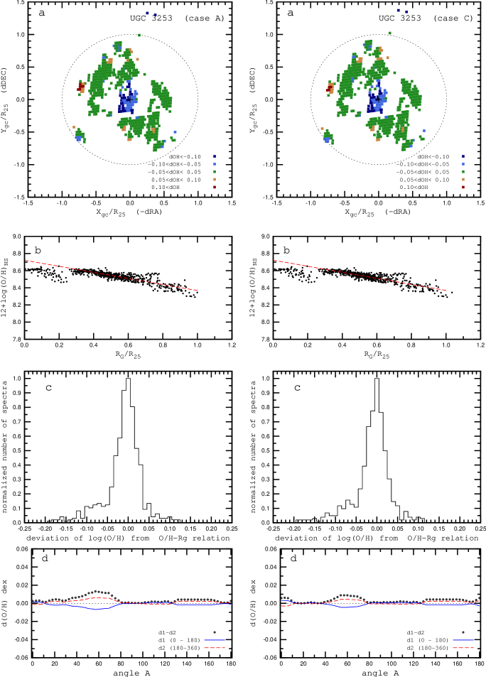
Figure 12: UGC 3253 is a galaxy with a possible bend in the radial abundance distribution. The oxygen abundances in the central part of the galaxy are systematically lower as compared to the general radial abundance trend. The panels and symbols are the same as in Fig. 4.

We have found that the radial abundance distribution across the disks of the majority of the galaxies of our sample can be well fitted by a single relation. In a subset of galaxies a bend in the radial abundance distribution across the disk may exist within the optical $R_{25}$ radius. Fig. 12 shows UGC 3253, which is a galaxy with a possible bend in the radial abundance distribution within the optical radius. The oxygen abundances in the central part of the galaxy are systematically lower as compared to the general radial abundance trend. Possible bends in the radial abundance distributions in other galaxies (a flattening or lowering in the central part) are reported in Table 2 (column 11). The decrease of the oxygen abundances in the central parts of a number of the CALIFA galaxies was first revealed by Sánchez et al. (2014). The nearly flat distribution in the innermost ($\la$0.2$R_{25}$) part of the galaxy NGC 628 was reported by Rosales-Ortega et al. (2011).

It should be noted that it is difficult to establish the exact value of the bend point due to the scatter in oxygen abundance values at any fixed radius and because the overall decrease of the oxygen abundance in the central part of a galaxy is small, within $\sim 0.1$ dex. Therefore, the break radius reported in Table 2 is an indicator that there is evidence for a decrease in the oxygen abundance in the central part of the galaxy rather than the exact value of the bend point.

The arguments for or/and against the existence of the break in the radial abundance gradients in the disks of spiral galaxies were discussed in many papers (Vilchez et al., 1988; Vila-Costas & Edmunds, 1992; Vilchez & Esteban, 1996; Pilyugin et al., 2003a, 2004; Bresolin et al., 2009, 2012; Goddard et al., 2011; Marino et al., 2012, 2016, among others) There is consensus is that the change in the radial abundance gradient can occur near the isophotal radius of a galaxy. The depressed gas metallicity in the central part of some CALIFA galaxies noticed by Sánchez et al. (2014) is confirmed here. Further investigations will strengthen or reject this picture.

Thus, there is evidence for a small change in the slope of the gradient (a flattening or decrease in the central part) in the disks of a number of galaxies.

4 Summary

We construct maps of the oxygen abundances across the disks of 88 CALIFA galaxies. The oxygen abundances were determined through the $C$ method using CALIFA DR2 spectra. Hence, here we use the empirical metallicity scale defined by H ii regions with oxygen abundances derived through the direct method ($T_{e}$ method). The position of the center of a galaxy (coordinates on the plate) were taken from the CALIFA DR2. The galaxy inclination and position angle of the major axis were determined from our analysis of $r$ band photometric maps of SDSS data release 9. The optical radii were determined from the radial surface brightness profiles in the SDSS $g$ and $r$ bands constructed on the basis of the photometric maps and converted to the Vega $B$ band.

We examine the global azimuthal asymmetry of the abundances in the disks of our target galaxies. The arithmetic mean of the deviations from the O/H $-R_{G}$ relation $d(O/H)_{1}$ for spaxels with azimuthal angles from $A$ to $A+180$ and mean deviation $d(O/H)_{2}$ for spaxels with azimuthal angles from $A+180$ to $A+360$ are determined for different positions of $A$. The maximum absolute value of the difference $d(O/H)_{1}-d(O/H)_{2}$ is used to specify the global azimuthal asymmetry in the abundance distribution across the galaxy.

The scatter around the O/H $-R_{g}$ relation for our sample of CALIFA galaxies is in the range of $\sim 0.02$ to $\sim 0.06$ dex. There is no significant global azimuthal asymmetry for our CALIFA sample. The values of the global azimuthal asymmetry are small, less than 0.05 dex for the bulk of target galaxies. These values can be attributed to the uncertainties in the photometry-map-based geometrical parameters of the galaxies, i.e., the uncertainties in the photometry-map-based geometrical parameters of a galaxy can make an appreciable (and possibly dominant) contribution to the obtained values of the azimuthal asymmetry.

We have found that the radial abundance distribution across the disks of the majority of the galaxies of our sample can be well fitted by a single relation. However, in eighteen of the galaxies in our sample, the oxygen abundances in the central part of the galaxies are systematically lower as compared to the general radial abundance trend. Although the decrease is rather well defined, its value is small, within $\sim$0.1 dex, and can be questioned taking into account the uncertainties of the abundances in the reference H ii regions. We note that the decrease of the oxygen abundances in the central parts of a number of the CALIFA galaxies was first revealed by Sánchez et al. (2014) and recently confirmed by Sánchez-Menguiano et al. (2016).

We estimated the geometric parameters of our galaxies (coordinates of the center, inclination and position angle of the major axis) from the analysis of the abundance map. The geometrical parameters are determined on the condition that the coefficient of the correlation between oxygen abundance and galactocentric distance is maximized or the scatter around the O/H – $R_{g}$ relation is minimized. Both these conditions result in the same values of the geometrical parameters. The photometry-map-based and the abundance-map-based geometrical parameters are relatively close to each other for the majority of our galaxies but the discrepancy is large for a few galaxies with a flat radial abundance gradient.

Appendix A Tables

Table 1 lists the general characteristics of each galaxy.
Column 1 gives its name. We have used the most widely used name for each galaxy. The galaxies are listed in the order of the name category, with the following categories in descending order:
NGC – New General Catalogue,
IC – Index Catalogue,
UGC – Uppsala General Catalog of Galaxies,
PGC – Catalogue of Principal Galaxies.
Columns 2 and 3 report the morphological type of the galaxy and the morphological type code $T$ from leda.
Column 4 lists the isophotal radius $R_{25}$ in arcmin of each galaxy. We determined the isophotal radius from the photometric maps in the SDSS $g$ and $r$ bands.
Column 5 gives the isophotal radius in kpc, estimated from the data in columns 4 and 6.
Column 6 reports the ned distances using flow corrections for Virgo, the Great Attractor, and Shapley Supercluster infall.

Table 2 lists the obtained properties of the oxygen abundance distributions in the disks of our sample of CALIFA galaxies. The inferred properties of each galaxy are given in two consecutive rows. In the first row, we report the geometrical parameters of the galaxies obtained from the analysis of the photometric map and the properties of the abundance distribution in the disk of the galaxies determined with deprojected galactocentric distances of spaxels for those geometrical parameters (case $A$ in the text and figures). In the second row, we report the geometrical parameters of the galaxies obtained from the analysis of the abundance map and the properties of the abundance distribution in the disk of the galaxy determined with deprojected galactocentric distances of spaxels for those geometrical parameters (case $C$ in the text). Column 1 gives the name of the galaxy. We have used the most widely used name for each galaxy. The galaxies are listed in the same order as in Table 1.
Columns 2 and 3 report the position of the galaxy center on the CALIFA exposure (the $X_{0}$ and $Y_{0}$ coordinates in spaxels).
Columns 4 and 5 give the galaxies’ inclination and the position angle of the major axes.
Columns 6 and 7 list the extrapolated central 12 + log(O/H)${}_{R_{0}}$ oxygen abundance and the radial oxygen abundance gradient expressed in terms of dex $R_{\rm 25}^{-1}$.
Column 8 reports the scatter of oxygen abundances around the general radial oxygen abundance trend within the optical $R_{25}$ radius of a galaxy.
Columns 9 and 10 give the global azimuthal asymmetry (maximum difference between the arithmetic means of the deviations from the O/H $-R_{g}$ relation for the opposite semicircle sectors) and the position of the dividing line (see panels $d$ in Fig. 4).
Column 11 lists the break radius if a bend in the radial abundance distribution exists.
Column 12 provides the number of the points in the abundance map for a galaxy.

Table 1: The adopted general properties of our sample of the CALIFA galaxies

Name	Type	T-type	$R_{25}$	$R_{25}$	Distance
			arcmin	kpc	Mpc
NGC 1	Sb	3.1	0.64	11.47	61.6
NGC 36	SABb	3.0	0.95	22.38	81.0
NGC 171	Sab	2.2	0.99	15.21	52.8
NGC 180	Sc	4.6	1.09	22.39	70.6
NGC 192	SBa	1.1	0.84	13.51	55.3
NGC 237	SABc	4.5	0.75	12.20	55.9
NGC 444	Sc	6.4	0.60	11.33	64.9
NGC 477	Sc	5.0	0.78	17.95	79.1
NGC 496	Sbc	4.0	0.69	16.16	80.5
NGC 776	SABa	2.5	0.77	14.67	65.5
NGC 1542	Sab	2.0	0.60	8.66	49.6
NGC 2253	Sc	5.8	0.77	11.49	51.3
NGC 2347	Sb	3.1	0.84	15.39	63.0
NGC 2410	Sb	3.0	0.87	16.97	66.3
NGC 2730	Sd	8.0	0.78	12.87	56.7
NGC 2906	Sc	5.9	0.84	8.19	33.5
NGC 2916	Sb	3.1	1.07	17.43	56.0
NGC 3381	SBb	3.2	0.93	7.79	22.8
NGC 3614	SABc	5.2	1.41	15.75	38.4
NGC 3811	SBc	5.8	0.86	12.40	49.0
NGC 3994	Sc	4.9	0.57	8.19	49.4
NGC 4185	SBbc	3.7	1.06	18.81	61.0
NGC 4210	Sb	3.0	0.86	10.81	43.2
NGC 4470	Sa	1.4	0.73	8.15	38.4
NGC 4644	Sb	3.1	0.52	11.18	73.9
NGC 5205	Sbc	3.5	0.87	7.82	30.9
NGC 5406	Sbc	3.9	0.92	21.14	79.0
NGC 5520	Sb	3.1	0.80	7.73	33.2
NGC 5614	Sab	1.7	1.09	19.47	61.4
NGC 5720	Sb	3.0	0.68	22.37	113.1
NGC 5888	Sbc	3.8	0.60	22.11	126.7
NGC 5947	SBbc	3.6	0.61	15.62	88.0
NGC 6004	Sc	4.9	0.90	15.92	60.8
NGC 6063	Sc	5.9	0.75	10.19	46.7
NGC 6132	Sab	2.0	0.56	12.46	76.5
NGC 6154	Sa	1.0	0.74	19.09	88.7
NGC 6478	Sc	4.9	0.81	23.05	98.0
NGC 6978	Sb	2.7	0.69	17.18	85.6
NGC 7311	Sab	2.0	0.81	14.80	62.8
NGC 7321	SBb	3.1	0.72	20.50	97.9
NGC 7466	Sb	3.1	0.58	17.26	102.3
NGC 7489	Sc	6.4	0.85	21.04	85.1
NGC 7549	Sc	5.9	0.83	15.65	64.8
NGC 7591	SBbc	3.6	0.79	15.54	67.6
NGC 7625	Sa	1.0	0.81	5.58	23.7
NGC 7631	Sb	3.1	0.77	11.54	51.5
NGC 7653	Sb	3.1	0.77	13.06	58.3
NGC 7716	Sb	3.0	0.96	9.94	35.6
NGC 7819	Sb	3.1	0.78	15.25	67.2
IC 674	Sab	2.0	0.59	18.64	108.6
IC 1199	Sbc	3.7	0.66	14.11	73.5
IC 1256	Sb	3.3	0.69	14.47	72.1
IC 1528	SBb	3.1	0.95	14.26	51.6
IC 2487	Sb	3.1	0.78	14.82	64.3
UGC 5	Sbc	3.9	0.64	18.23	97.9
UGC 809	Sc	5.9	0.49	8.07	56.6
UGC 1057	Sbc	4.0	0.55	13.58	84.9
UGC 1938	Sbc	4.0	0.52	12.83	84.8

Table 1: Continued

Name	Type	T-type	$R_{25}$	$R_{25}$	Distance
			arcmin	kpc	Mpc
UGC 2403	SBa	1.3	0.64	10.20	54.8
UGC 3107	Sbc	4.0	0.45	14.69	112.2
UGC 3253	Sb	3.0	0.70	12.12	59.5
UGC 3969	Sc	5.9	0.44	14.45	112.9
UGC 4132	Sbc	4.0	0.73	15.71	74.0
UGC 5396	Sc	5.8	0.65	15.05	79.6
UGC 5598	Sbc	3.8	0.47	11.36	83.1
UGC 8107	IB	9.9	0.70	24.33	119.5
UGC 8778	Sab	2.0	0.51	7.80	52.6
UGC 9067	Sab	2.0	0.56	18.95	116.3
UGC 9476	SABc	5.2	0.79	12.02	52.3
UGC 9665	Sbc	4.0	0.65	8.04	42.5
UGC 9873	Sc	5.3	0.46	11.28	84.3
UGC 9892	Sb	3.0	0.51	12.63	85.1
UGC 10331	Sb	3.1	0.58	11.34	67.2
UGC 10384	Sab	1.6	0.46	10.24	76.5
UGC 10710	Sb	3.0	0.57	20.05	120.9
UGC 10811	Sab	2.0	0.52	18.83	124.5
UGC 10972	Sc	5.9	0.65	13.35	70.6
UGC 11262	Sc	6.4	0.51	12.18	82.1
UGC 11649	SBa	1.0	0.77	12.39	55.3
UGC 11792	Sc	5.8	0.47	9.27	67.8
UGC 11982	SBc	6.0	0.40	7.82	67.2
UGC 12185	SBab	2.5	0.67	17.76	91.1
UGC 12224	Sc	5.9	0.87	12.33	48.7
UGC 12519	SBbc	4.5	0.68	11.85	59.9
UGC 12816	SABc	5.8	0.65	13.60	71.9
UGC 12864	SBb	3.1	0.74	13.69	63.6
PGC 1841	SBa	1.0	0.77	10.62	47.4
PGC 64373	Sd	8.0	0.63	15.01	81.9

Table 2: The obtained properties of the oxygen abundance distributions in the disks of the sample of CALIFA galaxies with available abundance maps.

Name	Center location		$i$	P.A.	(O/H)${}_{0}^{a}$	O/H gradient	$\sigma$(O/H)	Maximum azimuthal asymmetry		Break	Number of
	$X_{0}$	$Y_{0}$						amplitude	angle	radius	spectra
	spaxel	spaxel	degree	degree		dex $R_{25}^{-1}$	dex	dex	degree	$R_{25}$
1	2	3	4	5	6	7	8	9	10	11	12
NGC 1	38	36	45	101	8.61	-0.092	0.029	0.009	138		951
	36.7	36.5	61	87	8.61	-0.074	0.024	0.004	12
NGC 36	39	32	63	14	8.62	-0.107	0.033	0.015	102		524
	38.9	36.9	55	9	8.64	-0.171	0.035	0.011	75
NGC 171	35	34	20	161	8.67	-0.251	0.040	0.018	6	0.3	480
	36.5	35.5	40	75	8.66	-0.204	0.039	0.011	6
NGC 180	35	32	46	165	8.64	-0.198	0.037	0.015	165		906
	33.5	33.3	44	3	8.64	-0.192	0.036	0.006	120
NGC 192	38	33	65	168	8.64	-0.148	0.030	0.007	54		553
	38.7	34.1	71	158	8.64	-0.158	0.028	0.004	75
NGC 237	35	33	49	179	8.62	-0.302	0.037	0.024	171	0.2	1887
	32.9	33.1	45	1	8.62	-0.302	0.034	0.003	48
NGC 444	36	31	75	160	8.49	-0.207	0.050	0.019	51		813
	36.9	31.9	71	158	8.49	-0.240	0.050	0.006	48
NGC 477	33	30	57	142	8.63	-0.236	0.045	0.023	9		939
	35.3	31.3	56	141	8.63	-0.249	0.044	0.011	39
NGC 496	35	32	54	35	8.60	-0.276	0.047	0.054	18		1033
	38.1	33.1	58	33	8.62	-0.336	0.039	0.004	135
NGC 776	39	34	21	55	8.62	-0.075	0.035	0.022	30		1032
	32.7	29.7	29	19	8.62	-0.073	0.033	0.007	99
NGC 1542	37	33	66	129	8.56	-0.114	0.029	0.017	78		213
	38.9	35.9	72	126	8.57	-0.151	0.027	0.009	27
NGC 2253	40	33	43	127	8.62	-0.120	0.027	0.022	81		1275
	41.3	38.3	42	140	8.62	-0.133	0.024	0.003	150
NGC 2347	39	32	52	4	8.67	-0.329	0.038	0.030	162	0.3	1306
	36.7	32.9	51	4	8.67	-0.338	0.034	0.005	135
NGC 2410	37	32	72	35	8.62	-0.119	0.025	0.016	123		545
	40.5	26.7	75	34	8.62	-0.105	0.024	0.004	120
NGC 2730	38	31	43	86	8.51	-0.146	0.037	0.008	3		2689
	36.5	30.9	46	86	8.51	-0.144	0.037	0.004	75
NGC 2906	38	33	55	80	8.61	-0.052	0.021	0.005	99		1574
	39.1	33.9	67	73	8.61	-0.044	0.020	0.003	165
NGC 2916	37	33	51	17	8.63	-0.236	0.032	0.009	153		1028
	36.5	32.1	45	12	8.64	-0.267	0.031	0.006	156
NGC 3381	38	32	28	80	8.52	-0.191	0.037	0.025	150		2914
	33.3	33.9	32	94	8.53	-0.193	0.035	0.003	147
NGC 3614	38	33	55	101	8.59	-0.249	0.030	0.013	156		1218
	37.1	34.3	56	100	8.59	-0.254	0.029	0.005	27
NGC 3811	38	33	35	169	8.63	-0.196	0.024	0.007	81		1909
	38.3	31.7	37	182	8.63	-0.192	0.024	0.004	84
NGC 3994	37	33	59	7	8.55	-0.059	0.027	0.009	120		1496
	36.5	34.1	27	132	8.55	-0.078	0.026	0.007	60
NGC 4185	38	33	49	166	8.61	-0.135	0.036	0.020	144		416
	34.9	33.1	66	161	8.61	-0.085	0.034	0.009	21
NGC 4210	39	32	41	96	8.64	-0.192	0.024	0.010	36		1009
	38.1	31.5	40	88	8.63	-0.188	0.024	0.005	114
NGC 4470	34	36	48	0	8.47	-0.125	0.036	0.014	42		1680
	31.5	35.9	26	20	8.48	-0.167	0.035	0.005	0
NGC 4644	39	34	71	52	8.62	-0.084	0.029	0.011	174		597
	37.3	35.3	64	40	8.63	-0.113	0.029	0.003	57
NGC 5205	39	33	54	165	8.55	-0.020	0.036	0.010	93		381
	30.5	31.3	58	138	8.56	-0.030	0.035	0.007	84
NGC 5406	37	33	43	122	8.64	-0.147	0.035	0.010	141		1050
	38.9	33.5	52	109	8.64	-0.130	0.034	0.006	60
NGC 5520	39	33	59	65	8.60	-0.189	0.032	0.011	171		2316
	37.7	32.9	50	70	8.60	-0.218	0.030	0.002	129
NGC 5614	39	33	34	134	8.64	-0.184	0.041	0.014	63		741
	41.1	35.3	41	138	8.64	-0.169	0.040	0.006	150
NGC 5720	39	34	47	131	8.62	-0.186	0.048	0.018	168	0.3	344
	36.7	33.1	45	112	8.63	-0.204	0.046	0.009	0

Table 2: Continued

Name	Center location		$i$	P.A.	(O/H)${}_{0}^{a}$	O/H gradient	$\sigma$(O/H)	Maximum azimuthal asymmetry		Break	Number of
	$X_{0}$	$Y_{0}$						amplitude	angle	radius	spectra
	spaxel	spaxel	degree	degree		dex $R_{25}^{-1}$	dex	dex	degree	$R_{25}$
1	2	3	4	5	6	7	8	9	10	11	12
NGC 5888	38	32	52	154	8.61	-0.098	0.044	0.040	69		299
	45.5	44.5	67	149	8.61	-0.067	0.034	0.010	174
NGC 5947	43	36	31	63	8.66	-0.272	0.035	0.015	93		1404
	42.5	34.7	30	55	8.66	-0.267	0.034	0.005	45
NGC 6004	38	33	34	87	8.63	-0.161	0.036	0.012	66		1578
	36.1	31.5	43	90	8.63	-0.146	0.036	0.006	3
NGC 6063	38	34	56	156	8.58	-0.197	0.043	0.026	150		1795
	36.3	35.7	58	149	8.57	-0.176	0.037	0.007	126
NGC 6132	36	34	68	125	8.61	-0.306	0.051	0.046	147	0.2	875
	34.3	34.3	69	126	8.63	-0.332	0.044	0.008	93
NGC 6154	39	35	31	153	8.63	-0.152	0.026	0.010	159		438
	37.1	37.3	37	143	8.64	-0.175	0.025	0.005	90
NGC 6478	38	34	68	34	8.60	-0.157	0.034	0.014	66		1120
	37.3	33.5	71	37	8.59	-0.134	0.034	0.005	114
NGC 6978	38	33	67	128	8.60	-0.077	0.034	0.033	48		176
	41.3	38.5	62	126	8.62	-0.141	0.029	0.007	51
NGC 7311	38	33	60	12	8.62	-0.128	0.029	0.011	108		990
	38.1	35.7	66	11	8.62	-0.126	0.028	0.001	18
NGC 7321	37	33	46	13	8.62	-0.200	0.033	0.008	81	0.3	1745
	36.9	32.3	48	12	8.62	-0.197	0.032	0.003	171
NGC 7466	39	32	66	25	8.57	-0.109	0.032	0.023	123		798
	37.7	36.7	59	28	8.56	-0.110	0.029	0.003	96
NGC 7489	38	32	54	160	8.69	-0.628	0.062	0.034	144	0.2	1843
	37.7	33.3	59	162	8.69	-0.592	0.058	0.008	117
NGC 7549	38	34	67	18	8.58	-0.092	0.030	0.006	141		895
	36.7	34.5	23	164	8.59	-0.177	0.027	0.004	174
NGC 7591	38	33	54	156	8.63	-0.165	0.031	0.014	12		991
	36.7	33.7	49	151	8.63	-0.194	0.031	0.004	27
NGC 7625	36	32	30	22	8.59	-0.091	0.028	0.010	156		1620
	33.7	32.7	45	136	8.60	-0.101	0.027	0.003	96
NGC 7631	39	33	65	76	8.64	-0.198	0.033	0.009	12	0.2	1017
	40.7	32.7	67	75	8.64	-0.184	0.033	0.004	18
NGC 7653	37	33	31	175	8.63	-0.228	0.033	0.010	120		2226
	35.9	34.1	21	164	8.63	-0.242	0.032	0.004	162
NGC 7716	37	36	34	41	8.52	-0.058	0.032	0.005	78		1965
	35.3	36.9	61	15	8.52	-0.032	0.032	0.004	87
NGC 7819	34	34	55	104	8.60	-0.267	0.050	0.031	99		1184
	32.3	32.1	56	92	8.60	-0.269	0.044	0.008	177
IC 674	38	32	66	121	8.59	-0.157	0.045	0.028	141	0.2	386
	37.7	33.7	70	120	8.58	-0.120	0.041	0.013	3
IC 1199	38	33	68	164	8.62	-0.139	0.029	0.015	78		771
	38.5	35.5	63	162	8.62	-0.164	0.028	0.003	33
IC 1256	38	35	52	92	8.66	-0.273	0.040	0.011	141		1219
	37.3	34.9	51	88	8.66	-0.277	0.040	0.008	18
IC 1528	39	33	67	74	8.62	-0.319	0.048	0.017	3		1934
	37.5	33.1	66	76	8.62	-0.331	0.047	0.006	162
IC 2487	37	35	75	164	8.61	-0.235	0.038	0.023	150		867
	36.5	36.3	76	164	8.61	-0.236	0.034	0.007	60
UGC 5	38	32	60	46	8.59	-0.133	0.032	0.012	126	0.2	1189
	36.5	33.9	60	46	8.59	-0.128	0.031	0.005	177
UGC 809	32	31	77	24	8.46	-0.123	0.047	0.038	171	0.3	633
	34.1	30.5	72	28	8.48	-0.188	0.040	0.005	75
UGC 1057	36	32	71	152	8.63	-0.312	0.047	0.040	126	0.2	957
	35.9	33.7	68	156	8.63	-0.325	0.042	0.008	51
UGC 1938	35	29	73	155	8.62	-0.284	0.045	0.043	60	0.2	679
	36.9	31.9	71	155	8.64	-0.338	0.040	0.008	30
UGC 2403	33	32	67	152	8.65	-0.181	0.035	0.029	153		631
	31.1	33.1	57	151	8.66	-0.224	0.029	0.005	69
UGC 3107	36	32	76	73	8.60	-0.141	0.030	0.016	162		251
	34.9	32.7	74	67	8.59	-0.138	0.026	0.007	129

Table 2: Continued

Name	Center location		$i$	P.A.	(O/H)${}_{0}^{a}$	O/H gradient	$\sigma$(O/H)	Maximum azimuthal asymmetry		Break	Number of
	$X_{0}$	$Y_{0}$						amplitude	angle	radius	spectra
	spaxel	spaxel	degree	degree		dex $R_{25}^{-1}$	dex	dex	degree	$R_{25}$
1	2	3	4	5	6	7	8	9	10	11	12
UGC 3253	42	36	55	81	8.72	-0.354	0.031	0.013	57	0.3	622
	41.7	35.9	56	79	8.72	-0.352	0.030	0.009	54
UGC 3969	36	32	78	135	8.57	-0.091	0.025	0.006	18		320
	36.5	30.9	56	135	8.57	-0.117	0.021	0.004	129
UGC 4132	37	32	73	28	8.63	-0.147	0.021	0.015	72		1041
	37.1	33.7	70	29	8.63	-0.169	0.019	0.004	153
UGC 5396	38	31	70	156	8.61	-0.261	0.040	0.034	45		338
	36.3	30.5	66	151	8.63	-0.320	0.036	0.010	6
UGC 5598	38	32	73	36	8.56	-0.148	0.033	0.014	18		621
	37.1	32.3	69	35	8.56	-0.167	0.032	0.006	156
UGC 8107	39	33	68	52	8.57	-0.203	0.046	0.048	144		851
	35.7	35.3	63	40	8.58	-0.232	0.037	0.006	126
UGC 8778	36	32	74	118	8.55	-0.067	0.025	0.019	135		289
	37.5	34.9	79	124	8.56	-0.070	0.022	0.004	39
UGC 9067	39	32	62	13	8.66	-0.346	0.045	0.033	162	0.2	980
	38.3	32.9	56	11	8.68	-0.400	0.041	0.007	54
UGC 9476	37	33	48	125	8.55	-0.126	0.023	0.008	120		1220
	37.9	33.3	53	134	8.55	-0.118	0.022	0.004	114
UGC 9665	38	33	76	143	8.50	-0.086	0.038	0.018	159		970
	37.5	32.3	62	112	8.50	-0.092	0.031	0.008	54
UGC 9873	38	35	76	125	8.55	-0.140	0.034	0.022	177		534
	37.3	35.7	73	125	8.55	-0.159	0.032	0.005	36
UGC 9892	38	34	73	101	8.59	-0.177	0.028	0.012	105		616
	37.5	33.7	72	101	8.59	-0.182	0.027	0.004	54
UGC 10331	38	34	77	142	8.46	-0.167	0.054	0.046	45		1063
	35.7	32.5	61	142	8.47	-0.223	0.047	0.008	165
UGC 10384	39	33	76	91	8.59	-0.170	0.042	0.018	87		924
	39.1	34.3	57	94	8.60	-0.244	0.041	0.018	3
UGC 10710	39	36	75	148	8.58	-0.134	0.030	0.007	156		835
	38.9	36.3	77	148	8.59	-0.133	0.030	0.003	159
UGC 10811	39	33	68	93	8.66	-0.250	0.041	0.020	144	0.4	337
	36.7	33.1	70	88	8.68	-0.259	0.040	0.012	87
UGC 10972	37	32	75	54	8.62	-0.237	0.039	0.016	6	0.2	806
	35.9	32.7	77	53	8.62	-0.218	0.036	0.008	123
UGC 11262	37	33	68	48	8.57	-0.269	0.064	0.040	114		568
	36.3	34.7	60	53	8.58	-0.304	0.060	0.011	60
UGC 11649	38	33	38	70	8.65	-0.231	0.040	0.016	90	0.2	424
	38.5	31.1	33	58	8.65	-0.225	0.040	0.005	93
UGC 11792	40	32	77	160	8.56	-0.105	0.030	0.019	177		420
	39.3	32.1	79	160	8.56	-0.109	0.028	0.005	60
UGC 11982	39	31	78	169	8.44	-0.122	0.062	0.068	153		309
	37.7	33.5	74	164	8.48	-0.205	0.053	0.024	48
UGC 12185	39	33	62	147	8.56	-0.139	0.044	0.011	39		498
	37.7	33.3	68	157	8.57	-0.146	0.042	0.009	105
UGC 12224	38	32	24	47	8.59	-0.277	0.038	0.009	96		1069
	37.9	32.5	28	28	8.59	-0.274	0.038	0.007	96
UGC 12519	38	33	75	158	8.54	-0.129	0.030	0.024	114		1217
	37.7	35.7	71	155	8.55	-0.161	0.028	0.005	69
UGC 12816	39	34	53	140	8.51	-0.336	0.062	0.034	9		716
	36.9	32.9	56	144	8.52	-0.328	0.059	0.008	102
UGC 12864	37	35	64	106	8.51	-0.219	0.055	0.025	60		953
	35.9	33.7	63	87	8.51	-0.240	0.048	0.010	105
PGC 1841	34	32	66	165	8.59	-0.092	0.030	0.013	138		989
	33.1	33.9	70	169	8.60	-0.091	0.029	0.003	93
PGC 64373	39	32	67	159	8.65	-0.242	0.036	0.035	159		1060
	37.9	33.5	67	159	8.67	-0.282	0.031	0.005	75

^a in units of 12 + log(O/H)

References

- Ahn et al. (2012) Ahn C.P. et al., 2012, ApJS, 203, 21
- Aller (1984) Aller, L.H., 1984, Physics of Thermal Gaseous Nebulae, Reidel, Dordrecht
- Annibali et al. (2015) Annibali F., Tosi M., Pasquali A., Aloisi A., Mignoli M., Romano D., 2015, astro-ph 1505.05545
- Asari et al. (2007) Asari N. V., Cid Fernandes R., Stasińska G., et al. 2007, MNRAS, 381, 263
- Baldwin et al. (1981) Baldwin J.A., Phillips M.M., & Terlevich R. 1981, PASP, 93, 5
- Belfiore et al. (2015) Belfiore F., Maiolino R., Bundy K., et al., 2015, MNRAS, 449, 867
- Berg et al. (2012) Berg D.A., Skillman E.D., Marble A.R., 2012, ApJ, 754, 98
- Berg et al. (2013) Berg D.A., Skillman E.D., Garnett D.R., Croxall K.V., Marble A.R., Smith J.D., Gordon K., Kennicutt R.C., 2013, ApJ, 775, 128
- Berg et al. (2015) Berg D.A., Skillman E.D., Croxall K.V., Pogge R.W., Moustakas J., Johnson-Groh M., 2015, ApJ, 806, 16
- Bresolin et al. (2009) Bresolin F., Ryan-Weber E., Kennicutt R.C., Goddard Q., 2009, ApJ, 695, 580
- Bresolin (2011) Bresolin F., 2011, ApJ, 730, 129
- Bresolin et al. (2012) Bresolin F., Kennicutt R.C., Ryan-Weber E., 2012, ApJ, 750, 122
- Brown, Croxall & Pogge (2014) Brown J.S., Ceoxall K.V., Pogge R.W., 2014, ApJ, 792, 140
- Bruzual & Charlot (2003) Bruzual G., Charlot S., 2003, MNRAS, 344, 1000
- Cardelli, Clayton & Mathis (1989) Cardelli J. A., Clayton G. C., Mathis J. S., 1989, ApJ, 345, 245
- Cid Fernandes et al. (2005) Cid Fernandes R., Mateus A., Sodré L., Stasińska G., Gomes J. M., 2005, MNRAS, 358, 363
- Croxall et al. (2015) Croxall K.V., Pogge R.W., Berg D., Skillman E.D., Moustakas J., 2015, ApJ, 808, 42
- de Vaucouleurs et al. (1991) de Vaucouleurs, G., de Vaucouleurs, A., Corvin, H. G., et al. 1991, Third Reference Catalog of Bright Galaxies, New York: Springer Verlag (RC3)
- Dinerstein (1990) Dinerstein, H. L., 1990, in Thronson H.A., Shull J.M., eds., Proc. 2nd Teton Conf., The Interstellar Medium in Galaxies, Kluwer Academic Publishers, Dordrecht, p. 257
- Esteban et al. (2014) Esteban C., García-Rojas J., Carigi L., Peimbert M., Bresolin F., López-Sánchez A.R., Mesa-Delgado A., 2014, MNRAS, 443, 624
- García-Benito et al. (2014) García-Benito R. et al., 2014, A&A, 576, A135
- Goddard et al. (2011) Goddard Q., Bresolin F., Kennicutt R.C., Ryan-Weber E.V., Rosales-Ortega F.F., 2011, MNRAS, 412, 1246
- Gusev et al. (2012) Gusev A.S., Pilyugin L.S., Sakhibov F., Dodonov S.N., Ezhkova O.V., Khramtsova M.S., 2012, MNRAS, 424, 1930
- Haurberg, Rosenberg & Salzer (2013) Haurberg N.C., Rosenberg J., Salzer J.J., 2013, ApJ, 765, 66
- Haurberg et al. (2015) Haurberg N.C., Salzer J.J., Cannon J.M., Marshall M.V., 2015, ApJ, 800, 121
- Izotov et al. (1994) Izotov Y.I., Thuan T.X., Lipovetsky V.A., 1994, ApJ, 435, 647
- Izotov et al. (2006) Izotov Y.I., Stasińska G., Meynet G., Guseva N.G., Thuan T.X. 2006, A&A, 448, 955
- Izotov, Thuan & Guseva (2012) Izotov Y.I., Thuan T.X., Guseva N.G., 2012, A&A, 546, A122
- Kauffmann et al. (2003) Kauffmann G., Heckman T.M., Tremonti C., et al. 2003, MNRAS, 346, 1055
- Kennicutt & Garnett (1996) Kennicutt R.C., Garnett D.R., 1996, ApJ, 456, 504
- Kewley et al. (2001) Kewley L.J., Dopita M.A., Sutherland R.S., Heisler C.A., Trevena J. 2001 ApJ, 556, 121
- Kewley & Ellison (2008) Kewley L.J., Ellison S.L., 200, ApJ, 681, 1183
- Li, Bresolin & Kennicutt (2013) Li Y., Bresolin F., Kennicutt R.C., 2013, ApJ, 766, 17
- López-Sánchez & Esteban (2010) López-Sánchez Á.R., Esteban C., 2010, A&A, 517, A85
- Marino et al. (2012) Marino R.A., Gil de Paz A., Castillo-Morales A., et al., 2012, ApJ, 754, 61
- Marino et al. (2013) Marino R.A., Rosales-Ortega F.F., Sanchez S.F., et al., 2013, A&A, 559, 114
- Marino et al. (2016) Marino R.A., Gil de Paz A., Sanchez S.F., et al., 2016, A&A, 585, A47
- Martin & Belley (1996) Martin P., Belley J., 1996, ApJ, 468, 598
- Mateus et al. (2006) Mateus A., Sodré L., Cid Fernandes R., Stasińska G., Schoenell W., Gomes J. M., 2006, MNRAS, 370, 721
- Moustakas et al. (2010) Moustakas J., Kennicutt R.C., Tremonti C.A., Dale D.A., Smith J.-D.T., Calzetti D., 2010, ApJS, 190, 233
- Nicholls et al. (2014) Nicholls D.C., Dopita M.A., Sutherland R.S., Jerjen H., Kewley L.J., Basurah H., 2014, ApJ, 786, 155
- Osterbrock (1989) Osterbrock, D.E., 1989, Astrophysics of Gaseous Nebulae and Active Galactic Nuclei, University Science Books, Mill Valley, CA
- Pagel et al. (1992) Pagel B.E.J., Simonson E.A., Terlevich R.J., Edmunds M.G. 1992, MNRAS, 255, 325
- Pilyugin et al. (2001) Pilyugin L.S., 2001, A&A, 373, 56
- Pilyugin et al. (2003a) Pilyugin L.S., 2003a, A&A, 397, 109
- Pilyugin et al. (2003b) Pilyugin L.S., 2003, A&A, 399, 1003
- Pilyugin et al. (2004) Pilyugin L.S., Vílchez J.M., Contini T., 2004, A&A, 425, 849
- Pilyugin et al. (2006) Pilyugin L.S., Thuan T.X., Vílchez J.M., 2006, MNRAS, 367, 1139
- Pilyugin et al. (2007) Pilyugin L.S., Thuan T.X., Vílchez J.M., 2007, MNRAS, 376, 353
- Pilyugin et al. (2010) Pilyugin L.S., Vílchez J.M., Thuan T.X., 2010, ApJ, 720, 1738
- Pilyugin et al. (2012) Pilyugin L.S., Grebel E.K., & Mattsson L. 2012, MNRAS, 424, 2316
- Pilyugin et al. (2013) Pilyugin L.S., Lara-López M.A., Grebel E.K., et. al. 2013, MNRAS, 432, 1217
- Pilyugin et al. (2014a) Pilyugin L.S., Grebel E.K., Kniazev A.Y., 2014a, AJ, 147, 131
- Pilyugin et al. (2014b) Pilyugin L.S., Grebel E.K., Zinchenko I.A., Kniazev A.Y., 2014b, AJ, 148, 134
- Pilyugin et al. (2015) Pilyugin L.S., Grebel E.K., Zinchenko I.A., 2015, MNRAS, 450, 3254
- Pilyugin & Grebel (2016) Pilyugin L.S., Grebel E.K., 2016, MNRAS, 457, 3678