Scaling Up Sparse Support Vector Machines by Simultaneous Feature and Sample Reduction
Abstract
Sparse support vector machine (SVM) is a popular classification technique that can simultaneously learn a small set of the most interpretable features and identify the support vectors. It has achieved great successes in many real-world applications. However, for large-scale problems involving a huge number of samples and ultra-high dimensional features, solving sparse SVMs remains challenging. By noting that sparse SVMs induce sparsities in both feature and sample spaces, we propose a novel approach, which is based on accurate estimations of the primal and dual optima of sparse SVMs, to simultaneously identify the inactive features and samples that are guaranteed to be irrelevant to the outputs. Thus, we can remove the identified inactive samples and features from the training phase, leading to substantial savings in the computational cost without sacrificing the accuracy. Moreover, we show that our method can be extended to multi-class sparse support vector machines. To the best of our knowledge, the proposed method is the first static feature and sample reduction method for sparse SVMs and multi-class sparse SVMs. Experiments on both synthetic and real data sets demonstrate that our approach significantly outperforms state-of-the-art methods and the speedup gained by our approach can be orders of magnitude.
Keywords: screening, SVM, dual problem, optimization, classification
1 Introduction
Sparse support vector machine (SVM) (Bi et al., 2003; Wang et al., 2006) is a powerful technique that can simultaneously perform classification by margin maximization and variable selection via -norm penalty. The last few years have witnessed many successful applications of sparse SVMs, such as text mining (Joachims, 1998; Yoshikawa et al., 2014), bioinformatics (Narasimhan and Agarwal, 2013), and image processing (Mohr and Obermayer, 2004; Kotsia and Pitas, 2007). Many algorithms (Hastie et al., 2004; Fan et al., 2008; Catanzaro et al., 2008; Hsieh et al., 2008; Shalev-Shwartz et al., 2011) have been proposed to efficiently solve sparse SVM problems. However, the applications of sparse SVMs to large-scale learning problems, which involve a huge number of samples and extremely high-dimensional features, still remain challenging.
An emerging technique, called screening (El Ghaoui et al., 2012), has been shown to be promising in accelerating the training processes of large-scale sparse learning models. The essential idea of screening is to quickly identify the zero coefficients in the sparse solutions without solving any optimization problems such that the corresponding features or samples—that are called inactive features or samples—can be removed from the training phase. Then, we only need to perform optimization on the reduced data sets instead of the full data sets, leading to a substantial saving in the computational cost. Here, we need to emphasize that screening differs greatly from feature selection, although they look similar at the first glance. To be precise, screening is devoted to accelerating the training processes of many sparse models including Lasso, sparse SVMs, etc., while feature selection is the goal of these models. In the past few years, many screening methods are proposed for a large set of sparse learning techniques, such as Lasso (Tibshirani et al., 2012; Xiang and Ramadge, 2012; Wang et al., 2015), group Lasso (Ndiaye et al., 2016), -regularized logistic regression (Wang et al., 2014b), and SVMs (Ogawa et al., 2013). Most of the existing methods are in the same framework, i.e., estimating the optimum of the dual (resp. primal) problem and then developing the screening rules based on the estimations to infer which components of the primal (resp. dual) optimum are zero from the KKT conditions. The main differences among them are the techniques they use to develop their optima estimations and rules and the different sparse models they focus on. For example, SAFE (El Ghaoui et al., 2012) estimates the dual optimum by calculating the optimal value’s lower bound of the dual problem. The Lasso screening method (Wang et al., 2015) estimates the optimum based on the non-expensiveness (Bauschke et al., 2011) of the projection operator by noting that its dual problem boils down to finding the projection of a given point on a convex set. Moreover, a screening method is called static if it triggers its screening rules before training, and dynamic if during the training process. Empirical studies indicate that screening methods can lead to orders of magnitude of speedup in computation time.
However, most existing screening methods study either feature screening or sample screening individually and their applications have very different scenarios. Specifically, to achieve better performance (say, in terms of speedup), we favor feature screening methods when the number of features is much larger than the sample size , while sample screening methods are preferable when . Note that there is another class of sparse learning techniques, like sparse SVMs, which induce sparsities in both feature and sample spaces. All these screening methods tend to be helpless in accelerating the training process of these models with large and . We cannot address this problem by simply combining the existing feature and sample screening methods either. The reason is that they could mistakenly discard relevant data as they are specifically designed for different sparse models. Recently, Shibagaki et al. (2016) considered this issue and proposed a method to simultaneously identify the inactive features and samples in a dynamic manner, and they trigger their testing rule when there is a sufficient decrease in the duality gap during the training process. Thus, the method in Shibagaki et al. 2016 can discard more and more inactive features and samples as the training proceeds and one has small-scale problems to solve in the late stage of the training process. Nevertheless, the overall speedup is limited as the problems’ size can be large in the early stage of the training process. To be specific, the method in Shibagaki et al. 2016 depends heavily on the duality gap during the training process. The duality gap in the early stage can always be large, which makes the dual and primal estimations inaccurate and finally results in ineffective screening rules. Hence, it is essentially solving a large problem in the early stage. This will be verified in the experimental comparisons in Section 6 and similar results can also be found in the recent work (Massias et al., 2018), which merely focuses on Lasso.
In this paper, to address the limitations in the dynamic screening method, we propose a novel screening method that can Simultaneously identify Inactive Features and Samples (SIFS) for sparse SVMs in a static manner, and we only need to perform SIFS once before (instead of during) training. Thus, we only need to run the training algorithm on small-scale problems. The major technical challenge in developing SIFS is that we need to accurately estimate the primal and dual optima. The more accurate the estimations are, the more effective SIFS is in detecting inactive features and samples. Thus, our major technical contribution is a novel framework, which is based on the strong convexity of the primal and dual problems of sparse SVMs for deriving accurate estimations of the primal and dual optima (see Section 3). Another appealing feature of SIFS is the so-called synergistic effect (Shibagaki et al., 2016). Specifically, the proposed SIFS consists of two parts, i.e., Inactive Feature Screening (IFS) and Inactive Sample Screening (ISS). We show that discarding inactive features (resp. samples) identified by IFS (resp. ISS) leads to a more accurate estimation of the primal (resp. dual) optimum, which in turn dramatically enhances the capability of ISS (resp. IFS) in detecting inactive samples (resp. features). Thus, SIFS applies IFS and ISS in an alternating manner until no more inactive features and samples can be identified, leading to much better performance in scaling up large-scale problems than the application of ISS or IFS individually. Moreover, SIFS (see Section 4) is safe in the sense that the detected features and samples are guaranteed to be absent from the sparse representations. To the best of our knowledge, SIFS is the first static screening rule for sparse SVMs, which is able to simultaneously detect inactive features and samples. Experiments (see Section 6) on both synthetic and real data sets demonstrate that SIFS significantly outperforms the state-of-the-art (Shibagaki et al., 2016) in improving the training efficiency of sparse SVMs and the speedup can be orders of magnitude.
To demonstrate the flexibility of our proposed method SIFS, we extend its idea to multi-class sparse support vector machine (see Section 5), which also induces sparsities in both feature and sample spaces. Although multi-class sparse SVM has a very different structure and is more complex than sparse SVM, we will see that its dual problem has some similar properties (especially the strong convexity) with those of sparse SVM. Recall that SIFS we developed for sparse SVMs is mainly based on the strong convexity of the primal and dual problems. Therefore, the idea of SIFS is also applicable for multi-class sparse SVMs. Experimental results show that the speedup gained by SIFS in multi-class sparse SVMs can also be orders of magnitude.
For the convenience of presentation, we postpone the detailed proofs of all the theorems in this paper to the appendix. At last, we should point out that this journal paper is an extension of our own previous work (Zhang et al., 2017) published at the International Conference on Machine Learning (ICML) 2017.
Notations: Let , , and be , , and norms, respectively. We denote the inner product between vectors and by , and the -th component of by . Let for a positive integer . Given a subset of , let be the cardinality of . For a vector , let . For a matrix , let and , where and are the row and column of , respectively. For a scalar , we denote by . Let be the index vector, that is, if , otherwise . At last, we denote the set of nonnegative real numbers as .
2 Basics and Motivations
In this section, we briefly review some basics of sparse SVMs and then motivate SIFS via the KKT conditions. Specifically, we focus on an -regularized SVM with a smoothed hinge loss, which takes the form of
| (P∗) |
where is the parameter vector to be estimated, is the training set, , , , and are two positive parameters, and is the smoothed hinge loss, i.e.,
| (1) |
where .
Remark 1
We use the smoothed hinge loss instead of the vanilla one in order to make the objective of the Lagrangian dual problem of (P∗) strongly convex, which is needed in developing our accurate optima estimations. We should point out that the smoothed hinge loss is a pretty good approximation to the vanilla one with strong theoretical guarantees. See Section 5 in Shalev-Shwartz and Zhang 2016 for the details.
We present the Lagrangian dual problem of problem (P∗) and the KKT conditions in the following theorem, which play a fundamentally important role in developing our screening rules. We will not provide its proof in the appendix since it follows from Fenchel Duality (see Corollary 31.2.1 in Rockafellar, 1970) and a similar result can be found in Shibagaki et al. 2016.
Theorem 2
According to KKT-1 and KKT-2, we define 4 index sets:
which imply that
| (R) |
Thus, we call the -th feature inactive if . The samples in are the so-called support vectors and we call the samples in and inactive samples.
Suppose that we are given subsets of , , and . Then by the rules in (R), we can see that many coefficients of and are known. Thus, we may have much fewer unknowns to solve and the problem size can be dramatically reduced. We formalize this idea in Lemma 3.
Lemma 3
Given index sets , and , the followings hold:
, , ;
let , , and , where , , and . Then, solves the following scaled dual problem:
| (scaled-D∗) |
suppose that is known, then,
Lemma 3 indicates that, if we can identify index sets and and the cardinalities of and are much smaller than the feature dimension and the sample size , we only need to solve problem (scaled-D∗) that may be much smaller than problem (D∗) to exactly recover the optima and without sacrificing any accuracy.
However, we cannot directly apply Rules in (R) to identify subsets of , , and , as they require the knowledge of and that are usually unavailable. Inspired by the idea in El Ghaoui et al. 2012, we can first estimate regions and that contain and , respectively. Then, by denoting
| (4) | ||||
| (5) | ||||
| (6) |
since it is easy to know that , the rules in (R) can be relaxed as:
| (R1) | |||
| (R2) |
In view of Rules R1 and R2, we sketch the development of SIFS as follows.
-
Step 1:
Derive estimations and such that and , respectively.
- Step 2:
3 Estimate the Primal and Dual Optima
In this section, we first show that the primal and dual optima admit closed-form solutions for specific values of and (Section 3.1). Then, in Sections 3.2 and 3.3, we present accurate estimations of the primal and dual optima, respectively. We would like to point out that in order to extend the optimum estimation results below to multi-class sparse SVM and avoid redundancy, we consider the optimum estimations for the primal and dual problems in more general forms.
3.1 Effective Intervals of Parameters and
Below we show two things. One is that if the value of is sufficiently large, no matter what is, the primal solution is . The other is for any , if is large enough, the primal and dual optima admit closed-form solutions.
Lemma 4
Let and . Then,
(i) for and , we have
(ii) for all , we have
| (9) |
By Lemma 4, we only need to consider the cases where and .
3.2 Primal Optimum Estimation
In Section 1, we mention that the proposed SIFS consists of IFS and ISS, which can identify the inactive features and samples, respectively. We also mention that an alternating application of IFS and ISS can improve the estimation accuracy of the primal and dual optimum estimations, which can in turn make ISS and IFS more effective in identifying inactive samples and features, respectively. We would like to show that discarding inactive features by IFS leads to a more accurate estimation of the primal optimum.
We consider the following general problem (g-P∗):
| (g-P∗) |
where is smooth and convex. Exploiting the strong convexity of the objective function, we obtain the optimum estimation in the following lemma.
Lemma 5
For problem (P∗), let be the index set of inactive features identified by previous IFS steps. We have . Hence, we only need to find an estimation for . Since problem (P∗) is a special case of problem (g-P∗), given the reference solution and the set , from Lemma 5 we have:
| (12) |
It shows that lies in a ball of radius centered at . Note that, before we perform IFS, the set is empty and the second term on the right hand side of Eq. (11) is thus . If we apply IFS multiple times alternatively with ISS, the set will be monotonically increasing. Thus, Eq. (11) implies that the radius will be monotonically decreasing, leading to a more accurate primal optimum estimation.
3.3 Dual Optimum Estimation
We consider a general dual problem (g-D∗) below:
| (g-D∗) |
where and is smooth and convex. It is obvious that problem (g-D∗) can be reduced to problem (D∗) by letting and . The lemma below gives an optimum estimation of problem (g-D∗) based on the strong convexity of its objective function.
Lemma 6
We now turn back to problem (D∗). As it is a special case of problem (g-D∗), given the reference solution at and the index sets of inactive samples identified by the previous ISS steps and , using Lemma 6, we can obtain:
| (15) |
where and are defined by Eqs. (13) and (14) with , respectively. Therefore, lies in the ball . In view of Eq. (14), the index sets and monotonically increase and hence the last two terms on the right hand side of Eq. (14) monotonically increase when we perform ISS multiple times (alternating with IFS), which implies that the ISS steps can reduce the radius and thus improve the dual optimum estimation.
In addition, from both Lemmas 5 and 6, we can see that the radii of and can be potentially large when is very small, which may affect our estimation accuracy. We can sidestep this issue by letting the ratio be a constant. That is why we space the values of equally at the logarithmic scale on the parameter value path in the experiments.
4 The Proposed SIFS Screening Rule
We first present the IFS and ISS rules in Sections 4.1 and 4.2, respectively. Then, in Section 4.3, we develop the SIFS screening rule by an alternating application of IFS and ISS.
4.1 Inactive Feature Screening (IFS)
Suppose that and are known, we derive IFS to identify inactive features for problem (P∗) at by solving the optimization problem in Eq. (4) (see Section A.5 in the appendix):
| (16) |
where is given by Eq. (15) and and are the index sets of inactive features and samples that have been identified in previous screening processes, respectively. The next result shows the closed-form solution of problem (16).
Lemma 8
We are now ready to present the IFS rule.
Theorem 9
[Feature screening rule IFS] Consider problem (P∗). We suppose that and are known. Then:
-
(1)
the feature screening rule IFS takes the form of
(IFS) -
(2)
we can update the index set by
(17)
4.2 Inactive Sample Screening (ISS)
Similar to IFS, we derive ISS to identify inactive samples by solving the optimization problems in Eq. (5) and Eq. (6) (see Section A.7 in the appendix for details):
| (18) | |||
| (19) |
where is given by Eq. (12) and and are the index sets of inactive features and samples that have been identified in previous screening processes. We show that problems (18) and (19) admit closed-form solutions.
We are now ready to present the ISS rule.
Theorem 11
[Sample screening rule ISS] Consider problem (D∗) and suppose that and are known, then:
-
(1)
the sample screening rule ISS takes the form of
(ISS) -
(2)
we can update the index sets and by
(22) (23)
4.3 The Proposed SIFS Rule by An Alternating Application of IFS and ISS
In real applications, the optimal parameter values of and are usually unknown. To determine appropriate parameter values, common approaches, like cross validation and stability selection, need to solve the model over a grid of parameter values with and . This can be very time-consuming. Inspired by Strong Rule (Tibshirani et al., 2012) and SAFE (El Ghaoui et al., 2012), we develop a sequential version of SIFS in Algorithm 1.
Specifically, given the primal and dual optima and at , we apply SIFS to identify the inactive features and samples for problem (P∗) at . Then, we perform training on the reduced data set and solve the primal and dual optima at . We repeat this process until we solve problem (P∗) at all pairs of parameter values.
Note that we insert into every sequence ( see line 1 in Algorithm 1) to obtain a closed-form solution as the first reference solution. In this way, we can avoid solving problem at directly (without screening), which is time consuming. At last, we would like to point out that the values in SIFS can be specified by users arbitrarily.
SIFS applies ISS and IFS in an alternating manner to reinforce their capability in identifying inactive samples and features. In Algorithm 1, we apply ISS first. Of course, we can also apply IFS first. The theorem below demonstrates that the orders have no impact on the performance of SIFS.
Theorem 12
Given the optimal solutions and at as the reference solution pair at for SIFS, we assume SIFS with ISS first stops after applying IFS and ISS for times and denote the identified inactive features and samples as , and . Similarly, when we apply IFS first, the results are denoted as , and . Then, the followings hold:
(1) , and .
(2) with different orders of applying ISS and IFS, the difference between the times of ISS and IFS we need to apply in SIFS can never be larger than 1, that is, .
4.4 Discussion
After developing the proposed method SIFS above, we now turn to the related work discussion in order to highlight the differences between SIFS and the existing methods and also the novelty of our method, although we have mentioned some of them in the introduction section. We divide the previous work into two parts: screening for sparse SVM and for other sparse learning models.
To the best of our knowledge, the screening method in Shibagaki et al. 2016 is the only method besides our SIFS, which can simultaneously identify the inactive features and samples for sparse SVM. There are mainly three big differences between SIFS and this method. First, the techniques used in the optima estimations of SIFS and Shibagaki et al. 2016 are quite different. To be specific, the estimations in SIFS are developed by exploiting the reference solution pair and carefully studying the strong convexity of the objective functions and the optimum conditions of problems (P∗) and (D∗) at the current and reference parameter value pairs (see Lemmas 5 and 6 and also their proofs for the details). In contrast, Shibagaki et al. (2016) estimated the optima heavily based on the duality gap. As we mentioned in the introduction section, duality gap is usually large in the early stages and decreases gradually, which weakens its capability in the early stages and leads to a limited overall speedup. Second, algorithmically, Shibagaki et al. (2016) is dynamic while our method is static. In other words, Shibagaki et al. (2016) identifies the inactive features and samples during the training process, and in our method, we do this before the training process (see steps 6 to 11 in Algorithm 1), which means Shibagaki et al. (2016) needs to apply its screening rules for many times while we trigger SIFS only once. These two technical and algorithmic differences make our method outperform Shibagaki et al. (2016), which will be verified in the experimental section. At last, we theoretically prove that in the static scenario the orders of applying the feature and sample screening rules have no impact on the final performance, while Shibagaki et al. (2016) did not give the theoretical result accordingly in dynamic screening.
There are mainly three big differences between our SIFS and existing methods for other sparse learning models. First, these existing methods identify either features or samples individually and would be helpless in real applications involving a huge number of samples and extremely high-dimensional features, while SIFS identifies features and samples simultaneously. Second, technically, SIFS can incorporate the feature (resp. sample) screening results of the previous steps as the prior knowledge into the primal (reps. dual) optimum estimation to obtain a more accurate estimation. This is verified with a strong theoretical guarantee (see Lemmas 5 and 6). At last, we give a theoretical proof (see Sections 4.1 and 4.2) to show the existence of the synergistic effect between feature and sample screening for the first time in the static scenario.
Finally, we would like to point out that although the key ideas used in some of the screening methods including SIFS seem to be similar, they are developed specifically for the sparse models they focus on, which makes it nontrivial and even very difficult to reduce one method to another by simply resetting the loss and regularizer of the model. For example, SIFS cannot be reduced to Wang et al. (2014b) by setting and letting loss be the logistic loss, although both of their dual optimum estimations are based on the strong convexity of the objective. The reason is that they use the strong convexity in quite different ways due to their different dual problems including the feasible regions and the expressions of the dual objectives (see Theorem 2 in Wang et al., 2014b, Lemma 6 above, and their proofs for the details). Moreover, we cannot reduce SIFS to the methods (Ogawa et al., 2013; Wang et al., 2014a) for SVM by setting to be 0, since they are based on the convexity of the objective while SIFS exploits the strong convexity.
5 SIFS for Multi-class Sparse SVMs
In this section, we consider extending SIFS to multi-class sparse SVMs. We will briefly review the basics of multi-class sparse SVMs and then derive a series of theorems as we did for sparse SVMs above. Finally, we will present the detailed screening rule for multi-class sparse SVMs.
5.1 Basics of Multi-class Sparse SVMs
We focus on the -regularized multi-class SVM with a smoothed hinge loss, which takes the form of
| (m-P∗) |
where is the parameter vector to be estimated with . The loss function , with is the training data set of classes, , and is the smoothed hinge loss defined in Eq. (1).
The following theorem presents the Lagrangian dual problem of (m-P∗) and the KKT conditions, which are essential for developing the screening rules.
Theorem 13
As we did in Section 2, we can also define 3 index sets here:
which imply that
| (m-R) |
Suppose that we are given three subsets of , and , then we can infer the values of many coefficients of and via Rule m-R. The lemma below shows that the rest coefficients of and can be recovered by solving a small sized problem.
Lemma 14
Given index sets , and , the followings hold:
, , ;
let , , and , where , , and , then, solves the following scaled dual problem:
| (m-scaled-D∗) |
suppose that is known, then,
Given two estimations and for and , we can define three subsets of , and below as we did in the binary case to relax Rule m-R into the applicable version:
5.2 Estimate the Primal and Dual Optima
We first derive the effective intervals of the parameters and .
Lemma 15
Let and . Then:
(i) for and , we have
(ii) for all , we have
| (26) |
Hence, we only need to consider the cases with and .
Since problem (m-P∗) is a special case of problem (g-P∗) with , given the reference solution and the index set of the inactive features identified by the previous IFS steps, we can apply Lemma 5 to obtain the estimation for :
| (27) |
Moreover, noting that problem (m-D∗) is also a special case of problem (g-D∗), given the reference solution and the index sets of inactive samples identified by the previous ISS steps and , we can obtain an estimation for from Lemma 6:
| (28) |
where and are defined by Eqs. (13) and (14) with , respectively.
5.3 Screening Rule SIFS
Given the optima and , to derive the feature screening rule IFS, we need to solve the optimization problem below first:
| (29) |
where is the -th row of , is given by Eq. (28), and and are the index sets of the inactive features and samples identified in the previous screening process. We notice that this problem has exactly the same form as problem (16). Hence, from Lemma 8 we can obtain its closed-form solution directly. Now, from Rule m-R, we can obtain our IFS rule below.
-
•
The feature screening rule IFS takes the form of
(IFS) -
•
The index set can be updated by
(30)
Similarly, we need to solve the following problems to derive our sample screening rule ISS:
| (31) | |||
| (32) |
where is given by Eq. (27). We find that they can be solved by Lemma 10 directly. Therefore, we can obtain our sample screening rule ISS below.
-
•
The sample screening rule ISS takes the form of
(ISS) -
•
We can update the index sets and by
(35) (36)
The same as we did sparse SVM, we can also develop SIFS to reinforce the capabilities of ISS and IFS by applying them alternatively. The framework of SIFS for solving the model over a grid of parameter values here is the same as that in the case of sparse SVM, i.e. Algorithm 1, except for the different rules IFS and ISS, and the updates of , and .
In this version of SIFS, the order of applying IFS and ISS also has no impact on the final performance. Since the form of the theorem and its proof are nearly the same as that of Theorem 12, to avoid redundancy, we omit them in this section.
6 Experiments
We evaluate SIFS on both synthetic and real data sets in terms of three measurements: speedup, scaling ratio, and rejection ratio. Speedup is given by the ratio of the running time of the solver without screening to that with screening.
For sparse SVMs, scaling ratio is defined as , where , , , and are the numbers of inactive samples and features identified by SIFS, sample size, and feature dimension of the data set. From steps 6 to 11 in Algorithm 1, we can see that we trigger the rules ISS and IFS repetitively until no new features and samples are identified. We adopt the rejection ratios of the -th triggering of ISS and IFS defined as and to evaluate their performances in each triggering, where and are the numbers of inactive samples and features identified in the -th triggering of ISS and IFS. and are the numbers of inactive samples and features.
For multi-class sparse SVMs, we let scaling ratio be , where , , and and are the sample size and the feature dimension of the data set. The rejection ratios of the -th triggering of ISS and IFS are and , respectively, where , , and with , and are the increments of and in the -th triggering of the rules IFS and ISS. Please see Eqs. (30), (35), and (36) for the detailed definitions of , and .
Recall that, we can integrate SIFS with any solvers for problem (P∗). In this experiment, we use Accelerated Proximal Stochastic Dual Coordinate Ascent (AProx-SDCA) (Shalev-Shwartz and Zhang, 2016) as a baseline, as it is one of the state-of-the-arts. We choose the state-of-art screening method for sparse SVMs in Shibagaki et al. 2016 as another baseline only in the experiments of sparse SVMs, since it cannot be applied in multi-class sparse SVMs. As we mentioned in the introduction section that screening differs greatly from feature selection methods, it is not appropriate to make comparisons with feature selection methods.
For each data set, we solve problem (P∗) at a grid of turning parameter values. Specifically, we first compute by Lemma 4 and then select 10 values of that are equally spaced at the logarithmic scale of from to . Then, for each value of , we first compute by Lemma 4 and then select values of that are equally spaced at the logarithmic scale of from to . Thus, for each data set, we solve problem (P∗) at pairs of parameter values in total. We write the code in C++ along with Eigen library for numerical computations. We perform all the computations on a single core of Intel(R) Core(TM) i7-5930K 3.50GHz, 128GB MEM.
6.1 Simulation Studies with Spare SVMs
We evaluate SIFS on 3 synthetic data sets named syn1, syn2, and syn3 with sample and feature size . We present each data point as with and . We use Gaussian distributions , and to generate the data points, where and is the identity matrix. To be precise, for positive and negative points are sampled from and , respectively. For each entry in , it has chance to be sampled from and chance to be 0.


Fig. 1 shows the scaling ratios by ISS, IFS, and SIFS on the synthetic data sets at parameter values. We can see that IFS is more effective in scaling problem size than ISS, with scaling ratios roughly against . Moreover, SIFS, which is an alternating application of IFS and ISS, significantly outperforms ISS and IFS, with scaling ratios roughly . This high scaling ratios imply that SIFS can lead to a significant speedup.
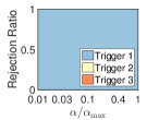
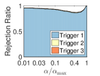
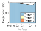
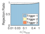
Due to the space limitation, we only report the rejection ratios of SIFS on syn2. Other results can be found in the appendix. Fig. 2 shows that SIFS can identify most of the inactive features and samples. However, few features and samples are identified in the second and later triggerings of ISS and IFS. The reason may be that the task here is so simple that one triggering is enough.
Table 1 reports the running times of solver without and with IFS, ISS and SIFS for solving problem (P∗) at pairs of parameter values. We can see that SIFS leads to significant speedups, that is, up to times. Taking syn2 for example, without SIFS, the solver takes more than two hours to solve problem (P∗) at pairs of parameter values. However, combined with SIFS, the solver only needs less than three minutes for solving the same set of problems. From the theoretical analysis in Shalev-Shwartz and Zhang 2016 for AProx-SDCA, we can see that its computational complexity rises proportionately to the sample size and the feature dimension . From this theoretical result, we can see that the results in Fig. 1 are roughly consistent with the speedups we achieved shown in Table 1.


| Data | Solver | ISS+Solver | IFS+Solver | SIFS+Solver | ||||||
| ISS | Solver | Speedup | IFS | Solver | Speedup | SIFS | Solver | Speedup | ||
| syn1 | 499.1 | 4.9 | 27.8 | 15.3 | 2.3 | 42.6 | 11.1 | 8.6 | 6.0 | 34.2 |
| syn2 | 8749.9 | 24.9 | 1496.6 | 5.8 | 23.0 | 288.1 | 28.1 | 92.6 | 70.3 | 53.7 |
| syn3 | 1279.7 | 2.0 | 257.1 | 4.9 | 2.2 | 33.4 | 36.0 | 7.2 | 9.5 | 76.8 |
6.2 Experiments with Sparse SVMs on Real Datasets
In this experiment, we evaluate the performance of SIFS on 5 large-scale real data sets: real-sim, rcv1-train, rcv1-test, url, and kddb, which are all collected from the project page of LibSVM (Chang and Lin, 2011). See Table 2 for a brief summary. We note that, the kddb data set has about 20 million samples with 30 million features.
Recall that, SIFS detects the inactive features and samples in a static manner, i.e., we perform SIFS only once before the training process and hence the size of the problem we need to perform optimization on is fixed. However, the method in Shibagaki et al. 2016 detects inactive features and samples in a dynamic manner (Bonnefoy et al., 2014), i.e., they perform their method along with the training process and thus the size of the problem would keep decreasing during the iterations. Thus, comparing SIFS with this baseline in terms of the rejection ratios is inapplicable. We compare the performance of SIFS with the method in Shibagaki et al. 2016 in terms of speedup, i.e., the speedup gained by these two methods in solving problem (P∗) at pairs of parameter values. The code of the method in Shibagaki et al. 2016 is obtained from (https://github.com/husk214/s3fs).
| Dataset | Feature size: | Sample size: | Classes |
|---|---|---|---|
| real-sim | 20,958 | 72,309 | 2 |
| rcv1-train | 47,236 | 20,242 | 2 |
| rcv1-test | 47,236 | 677, 399 | 2 |
| url | 3,231,961 | 2,396,130 | 2 |
| kddb | 29,890,095 | 19,264,097 | 2 |
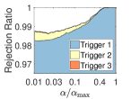

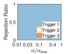

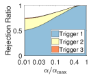
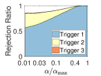
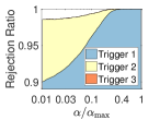
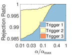
Fig. 3 shows the rejection ratios of SIFS on the real-sim data set (other results are in the appendix). In Fig. 3, we can see that some inactive features and samples are identified in the 2nd and 3rd triggerings of ISS and IFS, which verifies the necessity of the alternating application of ISS and IFS. SIFS is efficient since it always stops in 3 times of triggering. In addition, most of () the inactive features can be identified in the 1st triggering of IFS while identifying inactive samples needs to apply ISS two or more times. It may due to two reasons: 1) we run ISS first, which reinforces the capability of IFS due to the synergistic effect (see Sections 4.1 and 4.2), referring to the analysis below for further verification; 2) feature screening here may be easier than sample screening.
Table 3 reports the running times of solver without and with the method in Shibagaki et al. 2016 and SIFS for solving problem (P∗) at pairs of parameter values on real data sets. The speedup gained by SIFS is up to times on real-sim, rcv1-train and rcv1-test. Moreover, SIFS significantly outperforms the method in Shibagaki et al. 2016 in terms of speedup—by about to times faster on the aforementioned three data sets. For data sets url and kddb, we do not report the results of the solver as the sizes of the data sets are huge and the computational cost is prohibitive. Instead, we can see that the solver with SIFS is about times faster than the solver with the method in Shibagaki et al. 2016 on both data sets url and kddb. Let us take the data set kddb as an example. The solver with SIFS takes about hours to solve problem (P∗) for pairs of parameter values, while the solver with the method in Shibagaki et al. 2016 needs days to finish the same task.
| Data Set | Solver | Method in Shibagaki et al. 2016+Solver | SIFS+Solver | ||||
| Screen | Solver | Speedup | Screen | Solver | Speedup | ||
| real-sim | 3.93E+04 | 24.10 | 4.94E+03 | 7.91 | 60.01 | 140.25 | 195.00 |
| rcv1-train | 2.98E+04 | 10.00 | 3.73E+03 | 7.90 | 27.11 | 80.11 | 277.10 |
| rcv1-test | 1.10E+06 | 398.00 | 1.35E+05 | 8.10 | 1.17E+03 | 2.55E+03 | 295.11 |
| url | 3.50E+06 | 3.18E+04 | 8.60E+05 | 4.00 | 7.66E+03 | 2.91E+04 | 100 |
| kddb | 5.00E+06 | 4.31E+04 | 1.16E+06 | 4.00 | 1.10E+04 | 3.6E+04 | 100 |
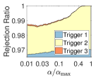


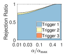
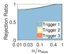
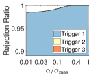
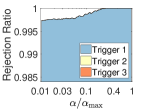
Verification of the Synergy Effect In Fig. 3, SIFS performs ISS (sample screening) first, while in Fig. 4, it performs IFS (feature screening) first. All the rejection ratios of the 1st triggering of IFS in Fig. 3(a)-3(d) where SIFS performs ISS first are much higher than (at least equal to) those in Fig. 4(a)-4(d) where SIFS performs IFS first. In turn, all the rejection ratios of the 1st triggering of ISS in Fig. 4(e)-4(h) where SIFS performs IFS first are also much higher than those in Fig. 3(e)-3(h) where SIFS performs ISS first. This demonstrates that the screening result of ISS can reinforce the capability of IFS and vice versa, which is the so called synergistic effect. At last, in Fig. 4 and Fig. 3, we can see that the overall rejection ratios at the end of SIFS are exactly the same. Hence, no matter which rule (ISS or IFS) we perform first in SIFS, SIFS has the same screening performances in the end, which verifies the conclusion we present in Theorem 12.
Performance in Solving Single Problems In the experiments above, we solve problem (P∗) at a grid of turning parameter values. This setting is meaningful and it arises naturally in various cases, such as cross validation (Kohavi, 1995) and feature selection (Meinshausen and Bühlmann, 2010; Yang et al., 2015). Therefore, the results above demonstrate that our method would be helpful in such real applications. We notice that sometimes one may be interested in the model at a specific parameter value pair. To this end, we now evaluate the performance of our method in solving a single problem. Due to the space limitation, we solve sparse SVM at 16 specific parameter values pairs on the real-sim data set for examples, To be precise, and each has 4 values of satisfying . For each , we construct a parameter value path with equally spaced at the logarithmic scale of between and , which implies that . Then we use AProx-SDCA integrated with SIFS to solve problem (P∗) at the parameter value pairs on the path one by one and report the total time cost. It can be expected that for far from , we need more points on the parameter value path in order to obtain higher rejection ratios and more significant speedups of SIFS and otherwise we need fewer ones. In this experiment, we fix at each for convenience. For comparison, we solve the problem at using AProx-SDCA with random initializations, which would be faster than solving all the problems on the path. Table 4 reports the speedups achieved by SIFS at these parameter value pairs. It shows that SIFS can still obtain significant speedups. In addition, compared with the results in Tables 1 and 3, we can see that our method is much better at solving a problem sequence than solving a single problem.
| 0.05 | 0.10 | 0.50 | 0.90 | |
|---|---|---|---|---|
| 0.05 | 6.31 | 7.14 | 21.04 | 146.66 |
| 0.10 | 6.14 | 7.18 | 21.83 | 156.63 |
| 0.50 | 5.75 | 7.18 | 20.99 | 154.60 |
| 0.90 | 6.39 | 7.66 | 23.16 | 173.56 |
6.3 Experiments with Multi-class Sparse SVMs
We evaluate SIFS for multi-class Sparse SVMs on 3 synthetic data sets (syn-multi1, syn-multi2, and syn-multi3) and 2 real data sets (news20 and rcv1-multiclass). Their statistics are given in Table 5.
The synthetic data sets are generated in a similar way as we did in Section 6.1. Each of them has classes and each class has samples. The data points of them can be written as , where with and . If belongs to the -th class, then is sampled from a Gaussian distribution with , and other components in are from . Each entry of has chance to be sampled from distribution and chance to be 0.
| Dataset | Feature size: | Sample size: | Classes |
|---|---|---|---|
| syn-multi1 | 1,000 | 10,000 | 5 |
| syn-multi2 | 10,000 | 10,000 | 5 |
| syn-multi3 | 10,000 | 1,000 | 5 |
| news20 | 3,993 | 62,060 | 20 |
| rcv1-multiclass | 47,236 | 15,564 | 53 |
Fig. 5 shows the scaling ratios of ISS, IFS, and SIFS on the synthetic data sets at pairs of parameter values. Similar to the results in sparse SVMs, SIFS totally surpasses IFS and ISS, with scaling ratios larger than at any parameter value pair against . Thus, we can expect significant speedups by integrating SIFS with the solver.


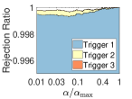
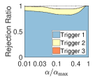
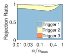
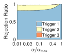
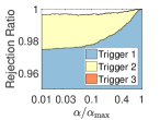
Fig. 6 and 7 present the rejection ratios of SIFS on the news20 data set (the results of other data sets can be found in the appendix). It indicates that, by alternatively applying IFS and ISS, we can finally identify most of the inactive samples () and features (). The synergistic effect between IFS and ISS can also be found in these figures.
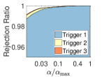
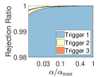


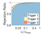
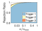


As a result of excellent performance of SIFS in identifying inactive features and samples, we observe significant speedups gained by SIFS in Table 6, which are up to 200 times on news20 and 300 times on syn-multi3. Specifically, on news20, the solver without any screening method takes about 97 hours to solve the problem at pairs of parameter values; however, integrated with SIFS, the solver only needs less than 0.5 hour for the same task. Moreover, Table 6 also indicates that the speedup gained by SIFS is much more significant than that gained by IFS and ISS. This demonstrates again the great benefit of alternatively applying IFS and ISS in SIFS. At last, we notice that the speedup gained by SIFS and IFS on syn-multi3 is far greater than those gained on syn-multi1 and syn-multi2. The reason is that the convergence rate of the solver in our problem may depend on the condition number of the data matrix. The dimension of in syn-multi3 is much larger than its sample size ( over ), which leads to a large condition number and a bad convergence rate. However, SIFS and IFS can remove the inactive features from the model, which can greatly improve the convergence rate of the solver by decreasing the condition number. This point can also be supported by the fact in the experiment on syn-multi3 that the solver with SIFS or IFS needs much fewer iterations to converge to the optima than that without SIFS or IFS.
| Data | Solver | ISS+Solver | IFS+Solver | SIFS+Solver | ||||||
|---|---|---|---|---|---|---|---|---|---|---|
| ISS | Solver | Speedup | IFS | Solver | Speedup | SIFS | Solver | Speedup | ||
| syn-multi1 | 9009 | 72 | 1233 | 6.9 | 90 | 388 | 18.9 | 178 | 83 | 34.5 |
| syn-multi2 | 105484 | 412 | 27661 | 3.8 | 920 | 2606 | 29.9 | 1936 | 893 | 37.3 |
| syn-multi3 | 78373 | 44 | 18341 | 4.3 | 84 | 337 | 186.2 | 203 | 59 | 299.9 |
| news20 | 350277 | 283 | 13950 | 24.6 | 1000 | 65175 | 5.3 | 1485 | 290 | 197.3 |
| rcv1-multiclass | 396205 | 793 | 44639 | 8.7 | 1620 | 33191 | 11.4 | 2850 | 1277 | 96.0 |
7 Conclusions
In this paper, we proposed a novel data reduction method SIFS to simultaneously identify inactive features and samples for sparse SVMs. Our major contribution is a novel framework for an accurate estimation of the primal and dual optima based on strong convexity. To the best of our knowledge, the proposed SIFS is the first static screening method that is able to simultaneously identify inactive features and samples for sparse SVMs. An appealing feature of SIFS is that all detected features and samples are guaranteed to be irrelevant to the outputs. Thus, the model learned on the reduced data is exactly identical to that learned on the full data. To show the flexibility of the proposed SIFS, we extended it to multi-class sparse SVMs. The experimental results demonstrate that, for both sparse SVMs and multi-class sparse SVMs, SIFS can dramatically reduce the problem size and the resulting speedup can be orders of magnitude. We plan to generalize SIFS to more complicated models, e.g., SVMs with a structured sparsity-inducing penalty.
Acknowledgments
This work was supported by the National Basic Research Program of China (973 Program) under Grant 2013CB336500, National Natural Science Foundation of China under Grant 61233011, and National Youth Top-notch Talent Support Program.
A Detailed Proofs and More Experimental Results
In this appendix, we first present the detailed proofs of all the theorems in the main paper and then report the rest experimental results which are omitted in the experimental section.
A.1 Proof for Lemma 3
Proof of Lemma 3:
1) It is the immediate conclusion of the analysis above.
2) After feature screening, the primal problem (P∗) is scaled into:
| (scaled--1) |
Thus, we can easily derive out the dual problem of (scaled--1):
| (scaled--1) |
and the KKT conditions:
| (scaled-KKT-1) | |||
| (scaled-KKT-2) |
Then, it is obvious that , since essentially, problem (scaled--1) can be derived by substituting 0 to the weights for the eliminated features in problem (P∗) and optimizing over the rest weights.
Since the solutions and satisfy the conditions (KKT-1) and (KKT-2) and for all , we know that and satisfy the conditions (scaled-KKT-1) and (scaled-KKT-2). Thus they are the solutions of problems (scaled--1) and (scaled--1). Then, due to the uniqueness of the solution of problem (scaled--1), we have
| (40) |
From 1) we have and . Therefore, from the dual problem (scaled-D∗), we can see that can be recovered from the following problem:
Since , the proof is therefore completed.
A.2 Proof for Lemma 4
Proof of Lemma 4:
(i) We prove this lemma by verifying that the solutions and satisfy the conditions (KKT-1) and (KKT-2).
Firstly, since , we have . Thus and satisfy the condition (KKT-1).
Then, for all , we have
Thus, and satisfy the condition (KKT-2). Hence, they are the solutions of the primal problem (P∗) and the dual problem (D∗), respectively.
A.3 Proof for Lemma 5
Proof of Lemma 5:
Due to the -strong convexity of the objective , we have
which are equivalent to
Adding the above two inequalities together, we obtain
| (41) |
Substituting the prior that into Eq. (41), we obtain
The proof is complete.
A.4 Proof for Lemma 6
Proof of Lemma 6: Firstly, we need to extend the definition of to :
| (44) |
Due to the strong convexity of objective , we have
Since , the above inequalities are equivalent to
Adding the above two inequalities, we obtain
That is equivalent to
| (45) |
That is
| (46) |
Substituting the priors that and into Eq. (46), we have
The proof is complete.
A.5 Proof for Lemma 8
A.6 Proof for Theorem 9
A.7 Proof for Lemma 10
A.8 Proof for Theorem 11
A.9 Proof for Theorem 12
Proof of Theorem 12:
(1) Given the reference solutions pair and , if we do ISS first in SIFS and apply ISS and IFS for infinite times. If after times of triggering, no new inactive features or samples are identified, then we can denote the sequence of , and as:
| (48) | |||
| (49) |
In the same way, if we do IFS first in SIFS and no new inactive features or samples are identified after times of triggering of ISS and IFS, then the sequence can be denoted as:
| (50) | |||
| (51) |
We first prove that and hold for all by induction.
1) When , the equalities and hold since .
2) If and hold, by the synergistic effect of ISS and IFS, we have that and hold.
Thus, and hold for all .
Similar to the analysis in (1), we can also prove that and hold for all .
Combining (1) and (2), we can acquire
| (52) | |||
| (53) | |||
| (54) | |||
| (55) | |||
| (56) | |||
| (57) |
By the first equality of Eqs. (49), (52), and (53), we can obtain . Similarly, we can obtain and .
Doing the same analysis for , we can obtain .
Hence, .
The proof is complete.
A.10 Proof for Theorem 13
Proof of Theorem 13:
We notice . By denoting , it is easy to verify that . Thus, the problem (m-P∗) can be rewritten as:
Let . The primal problem (P∗) is then equivalent to
The Lagrangian then becomes
| (58) |
We first consider the subproblem :
| (59) |
By substituting Eq. (59) into , we obtain
| (60) |
Then, we consider the problem :
| (64) | ||||
| (68) |
Thus, we have
| (71) |
Combining Eqs.(58), (60), and (71), we obtain the dual problem:
A.11 Proof for Lemma 14
A.12 Proof for Lemma 15
Proof of Lemma 15:
(i) We prove this lemma by verifying that the solutions and satisfy the conditions (m-KKT-1) and (m-KKT-2).
Firstly, since , we have . Thus, and satisfy the condition (m-KKT-1). Then, for all , we have
Thus, and satisfy the condition (m-KKT-2). Hence, they are the solutions of the primal problem (m-P∗) and the dual problem (m-D∗), respectively.
A.13 More Experimental Results
Below, we report the rejection ratios of SIFS on syn1 (Fig. 8), syn3 (Fig. 9), rcv1-train (Fig. 10), rcv1-test(Fig. 11), url (Fig. 12), kddb (Fig. 13), syn-multi1 (Fig. 14), syn-multi3 (Fig. 15), and rcv1-multiclass (Fig. 16), which are omitted in the main paper. In all the figures, the first row presents the rejection ratios of feature screening and the second row presents those of sample screening.


References
- Bauschke et al. (2011) Heinz H Bauschke, Patrick L Combettes, et al. Convex analysis and monotone operator theory in Hilbert spaces, volume 408. Springer, 2011.
- Bi et al. (2003) Jinbo Bi, Kristin Bennett, Mark Embrechts, Curt Breneman, and Minghu Song. Dimensionality reduction via sparse support vector machines. The Journal of Machine Learning Research, 3:1229–1243, 2003.
- Bonnefoy et al. (2014) Antoine Bonnefoy, Valentin Emiya, Liva Ralaivola, and Rémi Gribonval. A dynamic screening principle for the lasso. In Signal Processing Conference (EUSIPCO), 2014 Proceedings of the 22nd European, pages 6–10. IEEE, 2014.
- Catanzaro et al. (2008) Bryan Catanzaro, Narayanan Sundaram, and Kurt Keutzer. Fast support vector machine training and classification on graphics processors. In Proceedings of the 25th international conference on Machine learning, pages 104–111. ACM, 2008.
- Chang and Lin (2011) Chih-Chung Chang and Chih-Jen Lin. Libsvm: a library for support vector machines. ACM Transactions on Intelligent Systems and Technology (TIST), 2(3):27, 2011.
- El Ghaoui et al. (2012) Laurent El Ghaoui, Vivian Viallon, and Tarek Rabbani. Safe feature elimination in sparse supervised learning. Pacific Journal of Optimization, 8:667–698, 2012.
- Fan et al. (2008) Rong-En Fan, Kai-Wei Chang, Cho-Jui Hsieh, Xiang-Rui Wang, and Chih-Jen Lin. Liblinear: A library for large linear classification. The Journal of Machine Learning Research, 9:1871–1874, 2008.
- Hastie et al. (2004) Trevor Hastie, Saharon Rosset, Robert Tibshirani, and Ji Zhu. The entire regularization path for the support vector machine. The Journal of Machine Learning Research, 5:1391–1415, 2004.
- Hastie et al. (2015) Trevor Hastie, Robert Tibshirani, and Martin Wainwright. Statistical learning with sparsity: the lasso and generalizations. CRC Press, 2015.
- Hsieh et al. (2008) Cho-Jui Hsieh, Kai-Wei Chang, Chih-Jen Lin, S Sathiya Keerthi, and Sellamanickam Sundararajan. A dual coordinate descent method for large-scale linear svm. In Proceedings of the 25th international conference on Machine learning, pages 408–415. ACM, 2008.
- Joachims (1998) Thorsten Joachims. Text categorization with support vector machines: Learning with many relevant features. Springer, 1998.
- Kohavi (1995) Ron Kohavi. A study of cross-validation and bootstrap for accuracy estimation and model selection. In International Joint Conference on Artificial Intelligence, pages 1137–1145, 1995.
- Kotsia and Pitas (2007) Irene Kotsia and Ioannis Pitas. Facial expression recognition in image sequences using geometric deformation features and support vector machines. Image Processing, IEEE Transactions on, 16(1):172–187, 2007.
- Massias et al. (2018) Mathurin Massias, Joseph Salmon, and Alexandre Gramfort. Celer: a fast solver for the lasso with dual extrapolation. In International Conference on Machine Learning, pages 3321–3330, 2018.
- Meinshausen and Bühlmann (2010) Nicolai Meinshausen and Peter Bühlmann. Stability selection. Journal of the Royal Statistical Society: Series B (Statistical Methodology), 72(4):417–473, 2010.
- Mohr and Obermayer (2004) Johannes Mohr and Klaus Obermayer. A topographic support vector machine: Classification using local label configurations. In Advances in Neural Information Processing Systems, pages 929–936, 2004.
- Narasimhan and Agarwal (2013) Harikrishna Narasimhan and Shivani Agarwal. Svm pauc tight: a new support vector method for optimizing partial auc based on a tight convex upper bound. In Proceedings of the 19th ACM SIGKDD international conference on Knowledge discovery and data mining, pages 167–175. ACM, 2013.
- Ndiaye et al. (2016) Eugene Ndiaye, Olivier Fercoq, Alexandre Gramfort, and Joseph Salmon. Gap safe screening rules for sparse-group lasso. In D. D. Lee, M. Sugiyama, U. V. Luxburg, I. Guyon, and R. Garnett, editors, Advances in Neural Information Processing Systems 29, pages 388–396. Curran Associates, Inc., 2016.
- Ogawa et al. (2013) Kohei Ogawa, Yoshiki Suzuki, and Ichiro Takeuchi. Safe screening of non-support vectors in pathwise svm computation. In Proceedings of the 30th International Conference on Machine Learning, pages 1382–1390, 2013.
- Rockafellar (1970) Ralph Tyrell Rockafellar. Convex analysis. Princeton university press, 1970.
- Shalev-Shwartz and Zhang (2016) Shai Shalev-Shwartz and Tong Zhang. Accelerated proximal stochastic dual coordinate ascent for regularized loss minimization. Mathematical Programming, 155(1-2):105–145, 2016.
- Shalev-Shwartz et al. (2011) Shai Shalev-Shwartz, Yoram Singer, Nathan Srebro, and Andrew Cotter. Pegasos: Primal estimated sub-gradient solver for svm. Mathematical programming, 127(1):3–30, 2011.
- Shibagaki et al. (2016) Atsushi Shibagaki, Masayuki Karasuyama, Kohei Hatano, and Ichiro Takeuchi. Simultaneous safe screening of features and samples in doubly sparse modeling. In Proceedings of The 33rd International Conference on Machine Learning, 2016.
- Tibshirani et al. (2012) Robert Tibshirani, Jacob Bien, Jerome Friedman, Trevor Hastie, Noah Simon, Jonathan Taylor, and Ryan J Tibshirani. Strong rules for discarding predictors in lasso-type problems. Journal of the Royal Statistical Society: Series B (Statistical Methodology), 74(2):245–266, 2012.
- Wang et al. (2014a) Jie Wang, Peter Wonka, and Jieping Ye. Scaling svm and least absolute deviations via exact data reduction. In Proceedings of the 31st International Conference on Machine Learning (ICML-14), pages 523–531, 2014a.
- Wang et al. (2014b) Jie Wang, Jiayu Zhou, Jun Liu, Peter Wonka, and Jieping Ye. A safe screening rule for sparse logistic regression. In Advances in Neural Information Processing Systems, pages 1053–1061, 2014b.
- Wang et al. (2015) Jie Wang, Peter Wonka, and Jieping Ye. Lasso screening rules via dual polytope projection. Journal of Machine Learning Research, 16:1063–1101, 2015.
- Wang et al. (2006) Li Wang, Ji Zhu, and Hui Zou. The doubly regularized support vector machine. Statistica Sinica, pages 589–615, 2006.
- Xiang and Ramadge (2012) Zhen James Xiang and Peter J Ramadge. Fast lasso screening tests based on correlations. In Acoustics, Speech and Signal Processing (ICASSP), 2012 IEEE International Conference on, pages 2137–2140. IEEE, 2012.
- Yang et al. (2015) Tao Yang, Jie Wang, Qian Sun, Derrek P Hibar, Neda Jahanshad, Li Liu, Yalin Wang, Liang Zhan, Paul M Thompson, and Jieping Ye. Detecting genetic risk factors for alzheimer’s disease in whole genome sequence data via lasso screening. In Biomedical Imaging (ISBI), 2015 IEEE 12th International Symposium on, pages 985–989. IEEE, 2015.
- Yoshikawa et al. (2014) Yuya Yoshikawa, Tomoharu Iwata, and Hiroshi Sawada. Latent support measure machines for bag-of-words data classification. In Advances in Neural Information Processing Systems, pages 1961–1969, 2014.
- Zhang et al. (2017) Weizhong Zhang, Bin Hong, Wei Liu, Jieping Ye, Deng Cai, Xiaofei He, and Jie Wang. Scaling up sparse support vector machine by simultaneous feature and sample reduction. In Proceedings of The 34th International Conference on Machine Learning, pages 4016–4025, 2017.