Next-to-leading order QCD predictions for top-quark pair production with up to three jets

Abstract

We present theoretical predictions for the production of top-quark pairs with up to three jets at the next-to leading order in perturbative QCD. The relevant calculations are performed with S HERPA and O PEN L OOPS . To address the issue of scale choices and related uncertainties in the presence of multiple scales, we compare results obtained with the standard scale $H_{\mathrm{T}}/2$ at fixed order and the M I NLO procedure. Analyzing various cross sections and distributions for $t\bar{t}+0,1,2,3$ jets at the 13 TeV LHC we find a remarkable overall agreement between fixed-order and M I NLO results. The differences are typically below the respective factor-two scale variations, suggesting that for all considered jet multiplicities missing higher-order effects should not exceed the ten percent level.

1 Introduction

The top quark as the heaviest known elementary particle plays a fundamental role, both in the Standard Model and in new physics scenarios. Experimental analyses of Large Hadron Collider (LHC) data collected during run II will provide unprecedented reach at high energy and in exclusive phase space regions with associated production of jets and vector bosons or Higgs bosons. The production of a $t\bar{t}$ system in association with multiple jets plays an especially important role as a background to new physics searches and to various Higgs and Standard Model analyses. In particular, the precise theoretical control of $t\bar{t}+$multijet backgrounds is one of the most important prerequisites for the observation of top-quark production in association with a Higgs boson, which would give direct access to the top-quark Yukawa coupling. In addition, $t\bar{t}+$multijet production allows for powerful test of perturbative QCD and is also routinely exploited for the validation of Monte Carlo tools that are used in a multitude of LHC studies. All these analyses require theoretical predictions at the highest possible accuracy.

Inclusive top-quark pair production at hadron colliders has been computed fully differentially to next–to–next–to–leading order (NNLO) in the strong coupling expansion Czakon:2013goa ; Czakon:2015owf . Predictions for top-quark pair production in association with up to two jets are available at the next–to–leading order (NLO) Dittmaier:2007wz ; Bredenstein:2009aj ; Bredenstein:2010rs ; Bevilacqua:2009zn ; Bevilacqua:2010ve ; Bevilacqua:2011aa , and NLO calculations for inclusive top-quark pair production and in association with up to one or two jets were matched to parton showers in order to provide predictions at the particle level Frixione:2002ik ; Frixione:2007nw ; Kardos:2011qa ; Alioli:2011as ; Frederix:2012ps ; Kardos:2013vxa ; Cascioli:2013era ; Hoeche:2013mua ; Hoeche:2014qda ; Czakon:2015cla .

In this letter we report on the first computation of top-quark pair production with up to three jets at NLO QCD. At present only few scattering processes with more than six external legs are known at NLO Berger:2010zx ; Ita:2011wn ; Bern:2013gka ; Badger:2013yda ; Badger:2013ava ; Denner:2015yca ; Bevilacqua:2015qha ; Denner:2016jyo , and the calculation at hand is the first one that deals with a $2\to 5$ process with seven colored external particles including also heavy quarks. Detailed predictions are presented for $pp\to t\bar{t}+0,1,2,3$ jets at 13 TeV, both at the level of cross sections and differential distributions. We also investigate the scaling behavior of $t\bar{t}+$multijet cross sections with varying jet multiplicity.

The characteristic scales of $t\bar{t}+$multijet production, i.e. the invariant mass of the $t\bar{t}$ system and the transverse momentum threshold for jet production, are typically separated by more than one order of magnitude, while differential observables involve multiple scales, which can be distributed over more than two orders of magnitude. In this situation, finding renormalization and factorization scales that ensure a decent convergence of perturbative QCD for the widest possible range of observables is not trivial. Moreover, in the presence of a wide spectrum of scales, the usage of standard factor-two variations for the estimation of theoretical uncertainties due to missing higher-order effects becomes questionable. Motivated by these observations, to gain more insights into the scale dependence of $t\bar{t}+$multijet production and related uncertainties we compare a fixed-order calculation, with the standard scale choice $H_{\mathrm{T}}/2$, against results based on the M I NLO method Hamilton:2012np . The scale $H_{\mathrm{T}}/2$ was found to yield stable and reliable NLO predictions for $V+$multijet production Berger:2009ep , while the M I NLO method is especially well suited for multi-scale QCD processes, as it controls, through next-to-leading logarithmic (NLL) resummation, the various higher-order logarithms that emerge from soft and collinear effects in the presence of widely separated scales. The present study provides a first systematic comparison of the two approaches.

2 Details of the calculation

Our calculations are performed using the event generator S HERPA  Gleisberg:2003xi ; Gleisberg:2008ta in combination with O PEN L OOPS  Cascioli:2011va ; OLhepforge , a fully automated one-loop generator based on a numerical recursion that allows the fast evaluation of scattering amplitudes with many external particles. For the reduction to scalar integrals and for the numerical evaluation of the latter we used C UT T OOLS  Ossola:2007ax in combination with O NE LO OP  vanHameren:2010cp and, alternatively, the C OLLIER library Denner:2016kdg , which implements the methods of Denner:2002ii ; Denner:2005nn ; Denner:2010tr . Tree amplitudes are computed using C OMIX  Gleisberg:2008fv , a matrix-element generator based on the color-dressed Berends-Giele recursive relations Duhr:2006iq . Infrared singularities are canceled using the dipole subtraction method Catani:1996vz ; Catani:2002hc , as automated in C OMIX , with the exception of K- and P-operators that are taken from the implementation described in Gleisberg:2007md . C OMIX is also used for the evaluation of all phase-space integrals. Analyses are performed with the help of R IVET  Buckley:2010ar .

partonic channel \ $N$	0	1	2	3
$gg\to t\bar{t}+N\,g$	47	630	9’438	152’070
$u\bar{u}\to t\bar{t}+N\,g$	12	122	1’608	23’835
$u\bar{u}\to t\bar{t}u\bar{u}+(N-2)\,g$	–	–	506	6’642
$u\bar{u}\to t\bar{t}d\bar{d}+(N-2)\,g$	–	–	252	3’321

Table 1: Number of one-loop Feynman diagrams in representative partonic channels in $pp\to t\bar{t}+N$ jets for $N=0,1,2,3$.

We carry out a series of $pp\to t\bar{t}+N$ jet NLO calculations with $N=0,1,2,3$, taking into account the exact dependence on the number of colors, $N_{c}=3$. As an illustration of the rapid growth of complexity at high jet multiplicity, in Table 1 we list the number of one-loop Feynman diagrams that contribute to a few representative partonic channels. In addition to the presence of more than $10^{5}$ loop diagrams in the $gg\to t\bar{t}+3g$ channel, we note that also the very large number of channels not listed in Table 1 as well as the computation of real contributions pose very serious challenges in the $t\bar{t}+3$ jet calculation.

Proton–proton cross sections are obtained by using, both at LO and NLO, the CT14 NLO PDF set Dulat:2015mca with five active flavors, and the corresponding strong coupling. Matrix elements are computed with massless $b$-quarks, and top-quarks are kept stable. Hence, our results can be compared to data only upon reconstruction of the $t\bar{t}$ system and extrapolation of fiducial measurements to the full phase space. However, we expect the main features shown in our analysis to be present also in computations including top-quark decays and acceptance cuts. The latter will undoubtedly play a role, but the reduction of scale uncertainties is generic as long as the radiative phase space is not heavily restricted by experimental cuts. Apart from performing a direct analysis, we also provide Root NTuples Bern:2013zja that can be used in the future for more detailed studies including top-quark decays and matching to parton showers.

In our standard perturbative calculations we employ renormalization and factorization scales defined as $\mu_{\mathrm{R}}=\mu_{\mathrm{F}}=H_{\mathrm{T}}/2$, where $H_{\mathrm{T}}=\sum_{i}\sqrt{p_{\mathrm{T},i}^{2}+m_{i}^{2}}$, with the sum running over all (anti)top quarks and light partons, including also real radiation at NLO. Results generated in this manner are compared to alternative computations based on the M I NLO procedure Hamilton:2012np . To this end, we have realized a fully automated implementation of the M I NLO method in S HERPA .

3 M I NLO method and implementation

The M I NLO method can be regarded as a generalized scale setting approach that guarantees a decent perturbative convergence for differential multi-jet cross sections. This is achieved via appropriate scale choices Amati:1980ch and Sudakov form factors Catani:1991hj that resum NLL enhancements in the soft and collinear regions of phase space. To this end, in the case of $t\bar{t}+$multijet production, LO partonic events of type $ab\to t\bar{t}+N$ partons are recursively clustered back to a core process $\tilde{a}\tilde{b}\to t\bar{t}$ by means of a $k_{\mathrm{T}}$ jet algorithm Catani:1993hr . The resulting clustering history is interpreted as an event topology, where the $N$-jet final state emerges from the core process through a sequence of successive branchings that take place at the scales $q_{N},\ldots,q_{2},q_{1}$ and are connected by propagators. The nodal scales $q_{i}$ correspond to the $k_{\mathrm{T}}$ measure of the jet algorithm, and only $1\to 2$ branchings consistent with the QCD interaction vertices are allowed. In our implementation of the $k_{\mathrm{T}}$ jet algorithm we use the definition of $\Delta R$ given in Eq. (11) of Catani:1993hr and we set $\Delta R=0.4$. Typically, the $k_{\mathrm{T}}$ algorithm gives rise to ordered branching histories with $q_{1}<\dots<q_{N}<\mu_{\mathrm{core}}$, where $\mu_{\mathrm{core}}$ is the characteristic hard scale of the core process. However, also unordered branchings can occur. For instance, this can happen in the presence of jets with transverse momenta above $\mu_{\mathrm{core}}$. Since soft-collinear resummation does not make sense for such hard emissions, in our M I NLO implementation possible unordered clusterings are undone and alternative ordered configurations are considered. At the end, the branching history is restricted to ordered branchings $q_{1}<\dots<q_{\tilde{N}}<\mu_{\mathrm{core}}$, where $\tilde{N}=N-M$. The remaining $M$ jets that can not be clustered in an ordered way are treated as part of the core process, and $\mu_{\mathrm{core}}$ is evaluated according to the kinematics of the corresponding $t\bar{t}+M$ jet hard event.

At LO, the renormalization scale $\mu_{\mathrm{R}}$ is chosen according to the event branching history in such a way that

$$\left[\alpha_{\mathrm{s}}(\mu_{R})\right]^{N+2}=\left[\alpha_{\mathrm{s}}(\mu_{\mathrm{core}})\right]^{2+M}\prod_{i=1}^{\tilde{N}}\alpha_{\mathrm{s}}(q_{i}),$$ (1)

and in our calculation we set $\mu_{\mathrm{core}}=H_{\mathrm{T}}/2$.

The resummation of soft and collinear logarithms is achieved by dressing external and internal lines of the event topology by Sudakov form factors. At variance with the original formulation of M I NLO Hamilton:2012np , in our implementation we employ the symmetry of the LO DGLAP splitting functions, $P_{ab}(z)$, to define physical Sudakov form factors

$$\begin{split}&\Delta_{a}(Q_{0},Q)=\exp\left\{-\int_{Q_{0}}^{Q}\frac{{\rm d}q}{q}\frac{\alpha_{\mathrm{s}}(q)}{\pi}\sum_{b=q,g}\right.\\ &\quad\left.\int_{0}^{1-q/Q}{\rm d}z\left(z\,P_{ab}(z)+\delta_{ab}\frac{\alpha_{\mathrm{s}}(q)}{2\pi}\frac{2C_{a}}{1-z}K\right)\right\}\;,\end{split}$$ (2)

where Catani:1990rr

$$K=\left(\frac{67}{18}-\frac{\pi^{2}}{6}\right)C_{A}-\frac{10}{9}T_{R}\,n_{f}\;,$$ (3)

and $a=g,q$ corresponds to massless gluons and quarks, respectively. The representation (2) allows the interpretation of $\Delta_{a}(Q_{0},Q)$ in terms of no-branching probabilities between the scales $Q_{0}$ and $Q$.

Given a LO event topology with $\tilde{N}$ ordered branchings, the lowest branching scale, $q_{\mathrm{min}}=q_{1}$, is identified as resolution scale, and the $\tilde{N}$ emissions are supplemented by Sudakov form factors that render them exclusive w.r.t. any extra emissions above $q_{\mathrm{min}}$. This is achieved by dressing each external line of flavor $a=q,g$ connected with the $i$-th branching by a form factor $\Delta_{a}(q_{\mathrm{min}},q_{i})$, while internal lines that connect successive branchings $k<l$ are dressed by factors $\Delta_{a}(q_{\mathrm{min}},q_{l})/$ $\Delta_{a}(q_{\mathrm{min}},q_{k})$, which correspond to no-branching probabilities between $q_{k}$ and $q_{l}$ at resolution scale $q_{\mathrm{min}}$. For internal lines that connect branchings at $q_{k}$ to the core process analogous no-branching probabilities between $q_{k}$ and $\mu_{\mathrm{core}}$ are applied. Sudakov form factors along the incoming lines provide a NLL resummation that corresponds to the evolution of PDFs from the resolution scale $q_{\mathrm{min}}$ to the hard scale of the core process. Therefore, for consistency, PDFs are evaluated at the factorization scale $\mu_{\mathrm{F}}=q_{\mathrm{min}}$.

The generalization to NLO requires only two straightforward modifications of the LO algorithm. First, for what concerns the scale setting and Sudakov form factors, the contributions that live in the $N$-parton phase space, i.e. Born and one-loop contributions as well as all IR-subtraction terms, are handled exactly as in LO. Instead, real-emission events that lead to histories with $\tilde{N}+1\leq N+1$ ordered branchings at scales $q_{0}<q_{1}<\dots<q_{\tilde{N}}$ are handled as Born-like $\tilde{N}$-parton events with resolution scale $q_{\mathrm{min}}=q_{1}$, i.e. the softest branching at the scale $q_{0}$ is considered as unresolved and is simply excluded from the M I NLO procedure. In other words, the softest emission at NLO is not dressed with Sudakov form factors and does not enter the definitions of $\mu_{\mathrm{R}}$ and $\mu_{\mathrm{F}}$. Second, appropriate counterterms are introduced in order to subtract the overall $\mathcal{O}(\alpha_{\mathrm{s}})$ contribution from Sudakov form factors, such as to avoid double counting of NLO effects.

Concerning the treatment of top quarks a few extra comments are in order. Given the low rate at which top quarks radiate jets, such emissions are simply neglected in our implementation of the M I NLO procedure by excluding top quarks from the clustering algorithm. To quantify the uncertainty arising from this approach, we implemented an alternative algorithm that allows the combination of top quarks with other final-state partons in the massive Durham scheme Krauss:2003cr ; Rodrigo:2003ws . The difference between the two procedures is found to be about 10% at leading order and 5% at next-to-leading order for the observables studied here, and it is therefore smaller than the renormalization and factorization scale uncertainties. Finally, also the top quarks that enter the core process are dressed with Sudakov form factors $\Delta_{t}(q_{\mathrm{min}},\mu_{\mathrm{core}})$, which render them exclusive w.r.t. emissions above $q_{\mathrm{min}}$. To compute the Sudakov form factors $\Delta_{t}$, we include quark masses in the splitting functions, according to the method described in Krauss:2003cr ; Rodrigo:2003ws , using the corresponding extension of Eq. (2). This means in particular that we use the massive splitting functions from Catani:2000ef , the propagator corrections listed in Krauss:2003cr ; Rodrigo:2003ws , and we replace the two-loop cusp term $K\,2C_{F}/(1-z)$ by $K\,C_{F}(2/(1-z)-m^{2}/p_{i}p_{j})$ in the case of massive quark splittings $\widetilde{\imath\jmath}\to i,j$.

Scale uncertainties in the M I NLO framework are assessed through standard factor-two variations of $\mu_{\mathrm{R}}$ and $\mu_{\mathrm{F}}$. The renormalization scale is kept fixed in the Sudakov form factors but is varied as usual in the rest of the (N)LO cross section, including the counterterms that subtract the $\mathcal{O}(\alpha_{\mathrm{s}})$ parts of the Sudakov form factors at NLO. Variations $\mu_{\mathrm{F}}\to\xi_{\mathrm{F}}\,\mu_{\mathrm{F}}$ of the factorization scale are more subtle. They have to be applied at the level of PDFs and related NLO counterterms, as well as in the Sudakov form factors that depend on $q_{\mathrm{min}}=\mu_{\mathrm{F}}$. More precisely, $q_{\mathrm{min}}\to\xi_{\mathrm{F}}\,q_{\mathrm{min}}$ variations are applied only to Sudakov form factors associated with external and internal initial-state lines, and Sudakov form factors $\Delta_{a}(\xi_{\mathrm{F}}\,q_{\mathrm{min}},q_{k})$ are set to one when $\xi_{\mathrm{F}}\,q_{\mathrm{min}}$ exceeds $q_{k}$.

4 Predictions for the 13 TeV LHC

In the following we present selected predictions for $pp\to t\bar{t}+0,1,2,3$ jets at 13 TeV. We construct jets by clustering light partons with the anti-$k_{t}$ algorithm Cacciari:2008gp at $R=0.4$, and by default we select jets with pseudorapidity $|\eta_{\mathrm{jet}}|<2.5$ and a jet-$p_{\mathrm{T}}$ threshold of $25$ GeV. Unless stated otherwise, depending on the minimum number $N$ of jets that is required by the observable at hand, inclusive (N)LO or MI(N)LO calculations with $N$ jets are used.

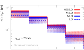
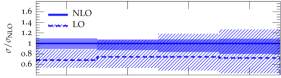
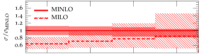
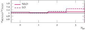
Figure 1: Inclusive $t\bar{t}+$multijet cross sections with a minimum number $N=0,1,2,3$ of jets at $p_{\mathrm{T},\mathrm{jet}}\geq$25 GeV. See the main text for details.

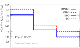
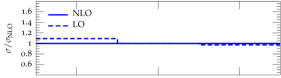
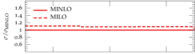
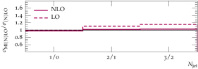
Figure 2: Ratios of $t\bar{t}+N$ jet over $t\bar{t}+(N-1)$ jet inclusive cross sections for $N=1,2,3$ and $p_{\mathrm{T},\mathrm{jet}}\geq$25 GeV.

The jet multiplicity distribution is presented in Fig. 1. The top panel displays four predictions, stemming from fixed-order LO and NLO calculations, and from M I NLO computations at LO and NLO (labeled ‘MILO’ and ‘MINLO’). The second panel shows the ratio between LO and NLO predictions at fixed order, while the third panel shows the ratio between MILO and MINLO predictions. The last panel shows the ratio between MINLO and NLO. The bands illustrate scale uncertainties estimated through independent factor-two rescaling of $\mu_{\mathrm{R}}$ and $\mu_{\mathrm{F}}$ excluding antipodal variations. Fixed-order predictions feature rather large NLO corrections of about $+50\%$ for all jet multiplicities, while M I NLO results feature steadily decreasing corrections for increasing $N_{\mathrm{jets}}$. In both cases, LO scale uncertainties tend to grow by more than $10\%$ at each extra jet emission, while (MI)NLO scale uncertainties are significantly reduced and the total width of the (MI)NLO variation bands is about 20–25% for all considered $N_{\mathrm{jets}}$ values. Comparing fixed-order NLO and MINLO predictions we observe a remarkable agreement at the level of 4–8%. This supports NLO and MINLO scale-uncertainty estimates based on factor-two variations and encourages the usage of either of the two calculations (NLO and MINLO) in practical applications.

$p_{\mathrm{T},\mathrm{jet}}\geq 25$ GeV	$\mathrm{LO}$	$\mathrm{NLO}$	$\mathrm{MILO}$	$\mathrm{MINLO}$	$\frac{\mathrm{MINLO}}{\mathrm{NLO}}$	$\frac{\mathrm{MINLO}}{\mathrm{MILO}}$	$\frac{\mathrm{NLO}}{\mathrm{LO}}$
$N_{\mathrm{jets}}$ $\geq 0$ $=0$	${440.46}(22)^{+28\%}_{-21\%}$	${644.34}(31)^{+9\%}_{-11\%}$ ${375.36}(41)^{+3\%}_{-15\%}$	${440.46}(22)^{+28\%}_{-21\%}$	${683.21}(31)^{+12\%}_{-12\%}$ ${394.66}(41)^{+2\%}_{-11\%}$	1.06 1.05	1.55 0.90	1.46 0.85
$N_{\mathrm{jets}}$ $\geq 1$ $=1$	${268.93}(9)^{+43\%}_{-28\%}$	${361.01}(26)^{+7\%}_{-13\%}$ ${249.52}(27)^{+2\%}_{-17\%}$	${267.86}(9)^{+36\%}_{-24\%}$	${373.94}(23)^{+11\%}_{-13\%}$ ${237.88}(25)^{+5\%}_{-14\%}$	1.04 0.95	1.40 0.89	1.34 0.93
$N_{\mathrm{jets}}$ $\geq 2$ $=2$	${111.32}(3)^{+59\%}_{-35\%}$	${149.43}(16)^{+8\%}_{-16\%}$ ${111.11}(16)^{+1\%}_{-18\%}$	${122.86}(4)^{+53\%}_{-32\%}$	${157.49}(16)^{+9\%}_{-16\%}$ ${103.98}(17)^{+5\%}_{-21\%}$	1.05 0.94	1.28 0.85	1.34 1.00
$N_{\mathrm{jets}}$ $\geq 3$ $=3$	${38.36}(2)^{+75\%}_{-40\%}$	${53.01}(10)^{+9\%}_{-20\%}$ ${41.12}(10)^{+0\%}_{-19\%}$	${48.89}(2)^{+71\%}_{-38\%}$	${57.43}(11)^{+4\%}_{-18\%}$ ${38.14}(12)^{+5\%}_{-38\%}$	1.08 0.93	1.17 0.78	1.38 1.07
$p_{\mathrm{T},\mathrm{jet}}\geq 40$ GeV	$\mathrm{LO}$	$\mathrm{NLO}$	$\mathrm{MILO}$	$\mathrm{MINLO}$	$\frac{\mathrm{MINLO}}{\mathrm{NLO}}$	$\frac{\mathrm{MINLO}}{\mathrm{MILO}}$	$\frac{\mathrm{NLO}}{\mathrm{LO}}$
$N_{\mathrm{jets}}$ $\geq 0$ $=0$	${440.46}(22)^{+28\%}_{-21\%}$	${644.34}(31)^{+9\%}_{-11\%}$ ${461.03}(36)^{+1\%}_{-4\%}$	${440.46}(22)^{+28\%}_{-21\%}$	${683.21}(31)^{+12\%}_{-12\%}$ ${483.40}(36)^{+1\%}_{-5\%}$	1.06 1.05	1.55 1.10	1.46 1.05
$N_{\mathrm{jets}}$ $\geq 1$ $=1$	${183.17}(7)^{+44\%}_{-28\%}$	${255.88}(20)^{+9\%}_{-13\%}$ ${201.57}(20)^{+0\%}_{-8\%}$	${200.36}(7)^{+35\%}_{-24\%}$	${276.63}(20)^{+10\%}_{-12\%}$ ${206.41}(21)^{+3\%}_{-7\%}$	1.08 1.02	1.38 1.03	1.40 1.10
$N_{\mathrm{jets}}$ $\geq 2$ $=2$	${54.23}(2)^{+59\%}_{-35\%}$	${76.13}(8)^{+10\%}_{-17\%}$ ${62.30}(8)^{+0\%}_{-12\%}$	${68.34}(2)^{+51\%}_{-31\%}$	${84.71}(10)^{+6\%}_{-14\%}$ ${63.60}(10)^{+2\%}_{-14\%}$	1.11 1.02	1.24 0.93	1.40 1.15
$N_{\mathrm{jets}}$ $\geq 3$ $=3$	${13.84}(1)^{+75\%}_{-40\%}$	${19.87}(4)^{+11\%}_{-21\%}$ ${16.61}(4)^{+1\%}_{-16\%}$	${20.55}(1)^{+68\%}_{-37\%}$	${22.70}(6)^{+2\%}_{-15\%}$ ${16.80}(6)^{+0\%}_{-33\%}$	1.14 1.01	1.10 0.82	1.44 1.20
$p_{\mathrm{T},\mathrm{jet}}\geq 60$ GeV	$\mathrm{LO}$	$\mathrm{NLO}$	$\mathrm{MILO}$	$\mathrm{MINLO}$	$\frac{\mathrm{MINLO}}{\mathrm{NLO}}$	$\frac{\mathrm{MINLO}}{\mathrm{MILO}}$	$\frac{\mathrm{NLO}}{\mathrm{LO}}$
$N_{\mathrm{jets}}$ $\geq 0$ $=0$	${440.46}(22)^{+28\%}_{-21\%}$	${644.34}(31)^{+9\%}_{-11\%}$ ${521.32}(33)^{+3\%}_{-6\%}$	${440.46}(22)^{+28\%}_{-21\%}$	${683.21}(31)^{+12\%}_{-12\%}$ ${547.02}(33)^{+5\%}_{-8\%}$	1.06 1.05	1.55 1.24	1.46 1.18
$N_{\mathrm{jets}}$ $\geq 1$ $=1$	${123.16}(5)^{+44\%}_{-29\%}$	${175.69}(15)^{+9\%}_{-14\%}$ ${149.59}(16)^{+3\%}_{-10\%}$	${142.02}(6)^{+35\%}_{-24\%}$	${195.17}(17)^{+9\%}_{-12\%}$ ${160.41}(17)^{+2\%}_{-8\%}$	1.11 1.07	1.37 1.13	1.43 1.21
$N_{\mathrm{jets}}$ $\geq 2$ $=2$	${26.06}(1)^{+59\%}_{-35\%}$	${37.47}(5)^{+11\%}_{-18\%}$ ${32.50}(5)^{+4\%}_{-14\%}$	${35.24}(2)^{+49\%}_{-30\%}$	${43.02}(8)^{+4\%}_{-13\%}$ ${35.10}(8)^{+2\%}_{-9\%}$	1.15 1.08	1.22 1.00	1.44 1.25
$N_{\mathrm{jets}}$ $\geq 3$ $=3$	${4.95}(0)^{+74\%}_{-40\%}$	${7.31}(2)^{+13\%}_{-22\%}$ ${6.41}(2)^{+5\%}_{-18\%}$	${7.97}(1)^{+65\%}_{-36\%}$	${8.61}(3)^{+1\%}_{-13\%}$ ${6.89}(3)^{+1\%}_{-27\%}$	1.18 1.07	1.08 0.86	1.48 1.29
$p_{\mathrm{T},\mathrm{jet}}\geq 80$ GeV	$\mathrm{LO}$	$\mathrm{NLO}$	$\mathrm{MILO}$	$\mathrm{MINLO}$	$\frac{\mathrm{MINLO}}{\mathrm{NLO}}$	$\frac{\mathrm{MINLO}}{\mathrm{MILO}}$	$\frac{\mathrm{NLO}}{\mathrm{LO}}$
$N_{\mathrm{jets}}$ $\geq 0$ $=0$	${440.46}(22)^{+28\%}_{-21\%}$	${644.34}(31)^{+9\%}_{-11\%}$ ${555.85}(32)^{+5\%}_{-8\%}$	${440.46}(22)^{+28\%}_{-21\%}$	${683.21}(31)^{+12\%}_{-12\%}$ ${584.21}(32)^{+7\%}_{-9\%}$	1.06 1.05	1.55 1.33	1.46 1.26
$N_{\mathrm{jets}}$ $\geq 1$ $=1$	${88.46}(4)^{+44\%}_{-29\%}$	${127.22}(12)^{+10\%}_{-14\%}$ ${112.89}(12)^{+5\%}_{-12\%}$	${104.19}(5)^{+34\%}_{-25\%}$	${142.99}(14)^{+9\%}_{-12\%}$ ${123.77}(14)^{+3\%}_{-9\%}$	1.12 1.10	1.37 1.19	1.44 1.28
$N_{\mathrm{jets}}$ $\geq 2$ $=2$	${14.33}(1)^{+59\%}_{-35\%}$	${20.81}(3)^{+11\%}_{-18\%}$ ${18.64}(3)^{+6\%}_{-15\%}$	${19.90}(1)^{+48\%}_{-30\%}$	${24.22}(4)^{+3\%}_{-12\%}$ ${20.71}(4)^{+1\%}_{-9\%}$	1.16 1.11	1.22 1.04	1.45 1.30
$N_{\mathrm{jets}}$ $\geq 3$ $=3$	${2.17}(0)^{+74\%}_{-40\%}$	${3.22}(1)^{+13\%}_{-22\%}$ ${2.91}(1)^{+8\%}_{-19\%}$	${3.59}(0)^{+63\%}_{-36\%}$	${3.85}(2)^{+1\%}_{-13\%}$ ${3.23}(2)^{+1\%}_{-23\%}$	1.19 1.11	1.07 0.90	1.48 1.34

Table 2: Inclusive ($N_{\mathrm{jets}}\geq n$) and exclusive ($N_{\mathrm{jets}}=n$) cross sections with $n=0,1,2,3$ jets and different transverse momentum thresholds, $p_{\mathrm{T},\mathrm{jet}}\geq 25,40,60,80$ GeV. Uncertainties represent the envelope of the independent $\mu_{\mathrm{R}}$ and $\mu_{\mathrm{F}}$ variations around the central value (antipodal variations excluded).

As demonstrated in Table 2, the good agreement between fixed-order NLO and MINLO results and the consistency of the observed NLO–MINLO differences with factor-two scale variations persist also for a range of other commonly used $p_{\mathrm{T},\mathrm{jet}}$-thresholds ATLAS-CONF-2015-065 . More precisely, for inclusive $t\bar{t}+N$ jet cross sections with jet-$p_{\mathrm{T}}$ thresholds of 25, 40, 65 and 80 GeV, MINLO predictions lie between 5% and 19% above NLO ones. The largest differences are observed at large jet multiplicity and for large $p_{\mathrm{T}}$-thresholds, in which case M I NLO cross sections feature significantly better perturbative convergence and smaller scale uncertainties as compared to fixed-order ones. In Table 2 also exclusive cross sections with exactly $N$ jets are presented. In that case, the difference between MINLO and NLO predictions varies between -7% and +11%. Apart from the zero-jet case, where the M I NLO approach is not well motivated, the MINLO/NLO ratio is almost independent of the number of jets and grows from 0.95 to 1.10 when the $p_{\mathrm{T}}$-threshold increases from 25 to 80 GeV. Similarly as in the inclusive case, at $p_{\mathrm{T}}$-thresholds above 40 GeV MINLO predictions for exclusive $N$-jet cross sections with $N\geq 2$ feature much better convergence and smaller scale uncertainties w.r.t. fixed order. However, for lower $p_{\mathrm{T}}$-thresholds the opposite is observed, and in the three-jet case the MINLO scale uncertainty becomes twice as large at the NLO one. This can be attributed to the fact that Sudakov logarithms related to the vetoing of NLO radiation are not resummed in the M I NLO approach. In spite of this caveat, the general agreement of fixed-order NLO and M I NLO results remains remarkably good for all considered observables.

Figure 2 shows ratios of inclusive $t\bar{t}+N$ jet cross sections for successive jet multiplicities. Due to the cancellation of various sources of experimental and theoretical uncertainties, such ratios are ideally suited for precision tests of QCD. Corresponding ratios have been widely studied in vector-boson plus multi-jet production Bern:2014fea ; Bern:2014voa , where a striking scaling behavior was observed at high jet multiplicity. In the case of $t\bar{t}$+multijet ratios involving up to three jets we find a moderate dependence on the number of jets but no clear scaling. This behavior is rather similar to scaling violations in $V+$ multijet production at lower multiplicity and, analogously as for $V+$ multijets, can be attributed to the suppression of important partonic channels in the zero-jet process at LO. In fact, quark–gluon channels are not active in $t\bar{t}$ production at LO. In addition, at LHC energies the gluonic initial state is strongly favored due to the parton luminosity and the $t$-channel enhancement of the $gg\to t\bar{t}$ cross section, such that the situation becomes similar to vector boson production, except for the difference of quark versus gluon initial states at LO. When adding additional jets, firstly quark–gluon initial states and secondly quark–quark initial states (including $t$-channel top-quark diagrams) are added, which contribute sizably to the cross section at larger invariant mass and/or transverse momentum. In order to test scaling hypotheses, it would therefore ultimately be necessary to compute the $t\bar{t}+4$ jet over $t\bar{t}+3$ jet ratio, and eventually the $t\bar{t}+5$ jet over $t\bar{t}+4$ jet ratio. This is out of reach of present technology, therefore we do not investigate the scaling behavior in more detail. Nevertheless, given the excellent agreement between MINLO and NLO predictions up to three jets, the ratios in Fig. 2 can be regarded as optimal benchmarks for precision tests.

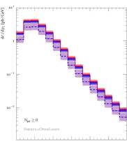
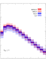
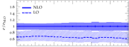
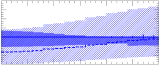
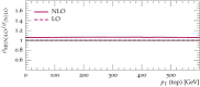
Figure 3: Distribution in the top-quark $p_{\mathrm{T}}$ for $pp\to t\bar{t}+0,1,2,3$ jets with $p_{\mathrm{T},\mathrm{jet}}\geq 25$ GeV.

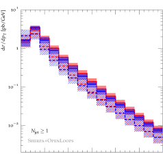
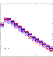
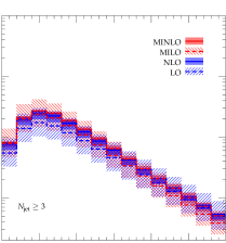
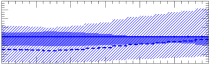
Figure 4: Distribution in the $p_{\mathrm{T}}$ of the $t\bar{t}$ system for $pp\to t\bar{t}+1,2,3$ jets with $p_{\mathrm{T},\mathrm{jet}}\geq 25$ GeV.

Figure 3 shows the transverse momentum spectrum of the top quark for varying jet multiplicities. From low to very high $p_{\mathrm{T}}$ NLO scale uncertainties remain at a similarly small level as for integrated cross sections. For $N_{\mathrm{jets}}\geq 1$, we observe significant shape corrections, which tend to decrease at high jet multiplicity in M I NLO, while in fixed order they remain important. We also observe a shape difference between fixed-order and M I NLO predictions, which tends to increase with increasing jet multiplicity but is clearly reduced at NLO. The overall agreement between fixed-order NLO and MINLO results is quite good, both in shape and normalization, with differences that lie within the individual scale uncertainties. Figure 4 shows the top-quark pair transverse momentum spectrum in 1-, 2- and 3-jet samples. We observe a large increase in the cross section between LO and NLO in the one-jet case, where the effect of additional radiation not modeled by the LO calculation is largest. At higher jet multiplicities correction effects tend to decrease. Fixed-order NLO uncertainties are similarly small as in Fig. 3, while MINLO scale uncertainties tend to be more pronounced in the tails. However, we find a very good overall agreement between fixed-order NLO and MINLO predictions, especially for $N_{\mathrm{jets}}\geq 2$ and 3.

The jet transverse momentum spectrum of the first, second and third jet, as predicted by $t\bar{t}+N$ jet calculations of corresponding jet multiplicity, is displayed in Fig. 5. In general we observe approximately constant NLO $K$-factors over the entire range of transverse momenta analyzed here, but in terms of perturbative convergence and scale uncertainties at NLO we find that the M I NLO approach performs better than fixed order. Comparing fixed-order and M I NLO results, at LO we find significant deviations that grow with $N_{\mathrm{jets}}$ and can reach 60% in the tails. Such differences are largely reduced by the transition to NLO. The fairly decent agreement between fixed-order NLO and MINLO results exemplifies nicely how the convergence of the perturbative series leads to a reduced dependence not only on constant scale variations, but also on the functional form of the scale.

Figure 6 shows inclusive $t\bar{t}+1,2,3$ jet predictions for the total light-jet transverse energy, which is defined as $H_{\mathrm{T}}^{\mathrm{jets}}=\sum_{j}|p_{\mathrm{T},j}|$, with the sum running over all reconstructed jets within acceptance. This observable is typically badly described by LO calculations, as a sizable fraction of events, especially at large $H_{\mathrm{T}}^{\mathrm{jets}}$, contains additional jets originating in initial-state radiation Rubin:2010xp . Correspondingly we observe a very large increase in the cross section between LO and NLO in the one-jet samples, where the effect of additional radiation not modeled by the calculation is largest. At higher jet multiplicities, the increase is smaller, but well visible. In M I NLO it tends to be more pronounced than at fixed order, and for $N_{\mathrm{jets}}\geq 3$ also MINLO uncertainties are larger than NLO ones. Nevertheless, we find good overall agreement between fixed-order NLO and MINLO predictions, independent of the jet multiplicity. However, given the strong sensitivity of $H_{\mathrm{T}}^{\mathrm{jets}}$ to multi-jet emissions, NLO or MINLO calculations with fixed jet multiplicity might significantly underestimate the effect of additional QCD radiation, and an approach like multijet merging at NLO Hoeche:2014qda would be more appropriate for this particular observable.

Studying differential distributions in several angular variables we did not find any sizable shape effect. We thus refrain from showing corresponding plots.

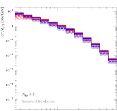
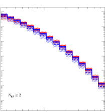
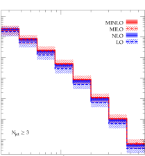
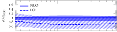
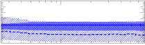
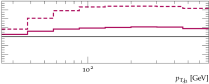
Figure 5: Distribution in the $p_{\mathrm{T}}$ of the $n$-th jet for $pp\to t\bar{t}+n$ jets with $p_{\mathrm{T},\mathrm{jet}}\geq 25$ GeV and $n=1,2,3$.

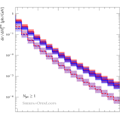
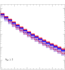
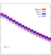
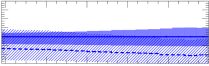
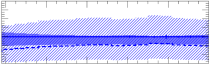
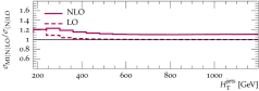
Figure 6: Distribution in the total transverse energy of light jets for $pp\to t\bar{t}+1,2,3$ jets with $p_{\mathrm{T},\mathrm{jet}}\geq 25$ GeV.

5 Conclusions

We have computed predictions for top-quark pair production with up to three additional jets at the next-to-leading order in perturbative QCD using the automated programs O PEN L OOPS and S HERPA . This is the first calculation of this complexity involving massive QCD partons in the final state. Given the multi-scale nature of $t\bar{t}$+multijet production, finding a scale that guarantees optimal perturbative convergence is not trivial. Moreover, standard factor-two scale variations might not provide a correct estimate of theoretical uncertainties related to missing higher-order effects. These issues have been addressed by comparing predictions obtained at fixed order using the scale $H_{\mathrm{T}}/2$ and, alternatively, with the M I NLO method. The hard scale $H_{\mathrm{T}}/2$ is known to yield good perturbative convergence for a large class of processes, while the M I NLO approach is more favorable from the theoretical point of view, as it implements NLL resummation for soft and collinear logarithms that emerge in the presence of large ratios of scales. For a rather wide range of observables at the 13 TeV LHC, we find very good agreement between the predictions generated at fixed order and with the M I NLO method. The differences turn out to be well consistent with factor-two scale variations of the respective predictions, which are typically at the 10% level. These observations suggest that the fixed-order NLO and MINLO approach can—to a large extent—be used interchangeably. Moreover, and most importantly, they significantly consolidate the picture of theoretical uncertainties that results from standard scale variations alone.

References

- (1) M. Czakon, P. Fiedler and A. Mitov, Phys.Rev.Lett. 110 (2013), 252004, [arXiv:1303.6254 [hep-ph]].
- (2) M. Czakon, D. Heymes and A. Mitov, Phys. Rev. Lett. 116 (2016), no. 8, 082003, [arXiv:1511.00549 [hep-ph]].
- (3) S. Dittmaier, P. Uwer and S. Weinzierl, Phys.Rev.Lett. 98 (2007), 262002, [hep-ph/0703120].
- (4) A. Bredenstein, A. Denner, S. Dittmaier and S. Pozzorini, Phys. Rev. Lett. 103 (2009), 012002, [arXiv:0905.0110 [hep-ph]].
- (5) A. Bredenstein, A. Denner, S. Dittmaier and S. Pozzorini, JHEP 03 (2010), 021, [arXiv:1001.4006 [hep-ph]].
- (6) G. Bevilacqua, M. Czakon, C. Papadopoulos, R. Pittau and M. Worek, JHEP 09 (2009), 109, [arXiv:0907.4723 [hep-ph]].
- (7) G. Bevilacqua, M. Czakon, C. Papadopoulos and M. Worek, Phys. Rev. Lett. 104 (2010), 162002, [arXiv:1002.4009 [hep-ph]].
- (8) G. Bevilacqua, M. Czakon, C. G. Papadopoulos and M. Worek, Phys. Rev. D84 (2011), 114017, [arXiv:1108.2851 [hep-ph]].
- (9) S. Frixione and B. R. Webber, JHEP 06 (2002), 029, [hep-ph/0204244].
- (10) S. Frixione, P. Nason and G. Ridolfi, JHEP 09 (2007), 126, [arXiv:0707.3088 [hep-ph]].
- (11) A. Kardos, C. Papadopoulos and Z. Trocsanyi, Phys.Lett. B705 (2011), 76–81, [arXiv:1101.2672 [hep-ph]].
- (12) S. Alioli, S.-O. Moch and P. Uwer, JHEP 01 (2012), 137, [arXiv:1110.5251 [hep-ph]].
- (13) R. Frederix and S. Frixione, JHEP 12 (2012), 061, [arXiv:1209.6215 [hep-ph]].
- (14) A. Kardos and Z. Trócsányi, J. Phys. G41 (2014), 075005, [arXiv:1303.6291 [hep-ph]].
- (15) F. Cascioli, P. Maierhoefer, N. Moretti, S. Pozzorini and F. Siegert, Phys. Lett. B734 (2014), 210–214, [arXiv:1309.5912 [hep-ph]].
- (16) S. Höche, J. Huang, G. Luisoni, M. Schönherr and J. Winter, Phys.Rev. D88 (2013), 014040, [arXiv:1306.2703 [hep-ph]].
- (17) S. Hoeche, F. Krauss, P. Maierhoefer, S. Pozzorini, M. Schonherr and F. Siegert, Phys. Lett. B748 (2015), 74–78, [arXiv:1402.6293 [hep-ph]].
- (18) M. Czakon, H. B. Hartanto, M. Kraus and M. Worek, JHEP 06 (2015), 033, [arXiv:1502.00925 [hep-ph]].
- (19) C. F. Berger, Z. Bern, L. J. Dixon, F. Febres-Cordero, D. Forde, T. Gleisberg, H. Ita, D. A. Kosower and D. Maître, Phys. Rev. Lett. 106 (2011), 092001, [arXiv:1009.2338 [hep-ph]].
- (20) H. Ita, Z. Bern, L. J. Dixon, F. Febres-Cordero, D. A. Kosower and D. Maître, Phys.Rev. D85 (2012), 031501, [arXiv:1108.2229 [hep-ph]].
- (21) Z. Bern, L. Dixon, F. Febres Cordero, S. Höche, H. Ita, D. A. Kosower, D. Maître and K. J. Ozeren, Phys.Rev. D88 (2013), 014025, [arXiv:1304.1253 [hep-ph]].
- (22) S. Badger, B. Biedermann, P. Uwer and V. Yundin, Phys.Rev. D89 (2013), 034019, [arXiv:1309.6585 [hep-ph]].
- (23) S. Badger, A. Guffanti and V. Yundin, JHEP 1403 (2014), 122, [arXiv:1312.5927 [hep-ph]].
- (24) A. Denner and R. Feger, JHEP 11 (2015), 209, [arXiv:1506.07448 [hep-ph]].
- (25) G. Bevilacqua, H. B. Hartanto, M. Kraus and M. Worek, Phys. Rev. Lett. 116 (2016), no. 5, 052003, [arXiv:1509.09242 [hep-ph]].
- (26) A. Denner and M. Pellen, arXiv:1607.05571 [hep-ph].
- (27) K. Hamilton, P. Nason and G. Zanderighi, JHEP 1210 (2012), 155, [arXiv:1206.3572 [hep-ph]].
- (28) C. F. Berger, Z. Bern, L. J. Dixon, F. Febres-Cordero, D. Forde, T. Gleisberg, H. Ita, D. A. Kosower and D. Maître, Phys. Rev. D80 (2009), 074036, [arXiv:0907.1984 [hep-ph]].
- (29) T. Gleisberg, S. Höche, F. Krauss, A. Schälicke, S. Schumann and J. Winter, JHEP 02 (2004), 056, [hep-ph/0311263].
- (30) T. Gleisberg, S. Höche, F. Krauss, M. Schönherr, S. Schumann, F. Siegert and J. Winter, JHEP 02 (2009), 007, [arXiv:0811.4622 [hep-ph]].
- (31) F. Cascioli, P. Maierhöfer and S. Pozzorini, Phys.Rev.Lett. 108 (2012), 111601, [arXiv:1111.5206 [hep-ph]].
- (32) F. Cascioli, J. Lindert, P. Maierhöfer and S. Pozzorini, The OpenLoops one-loop generator, publicly available at http://openloops.hepforge.org.
- (33) G. Ossola, C. G. Papadopoulos and R. Pittau, JHEP 0803 (2008), 042, [arXiv:0711.3596 [hep-ph]].
- (34) A. van Hameren, Comput.Phys.Commun. 182 (2011), 2427–2438, [arXiv:1007.4716 [hep-ph]].
- (35) A. Denner, S. Dittmaier and L. Hofer, arXiv:1604.06792 [hep-ph].
- (36) A. Denner and S. Dittmaier, Nucl. Phys. B658 (2003), 175–202, [hep-ph/0212259].
- (37) A. Denner and S. Dittmaier, Nucl. Phys. B734 (2006), 62–115, [arXiv:hep-ph/0509141 [hep-ph]].
- (38) A. Denner and S. Dittmaier, Nucl. Phys. B844 (2011), 199–242.
- (39) T. Gleisberg and S. Höche, JHEP 12 (2008), 039, [arXiv:0808.3674 [hep-ph]].
- (40) C. Duhr, S. Höche and F. Maltoni, JHEP 08 (2006), 062, [hep-ph/0607057].
- (41) S. Catani and M. H. Seymour, Nucl. Phys. B485 (1997), 291–419, [hep-ph/9605323].
- (42) S. Catani, S. Dittmaier, M. H. Seymour and Z. Trocsanyi, Nucl. Phys. B627 (2002), 189–265, [hep-ph/0201036].
- (43) T. Gleisberg and F. Krauss, Eur. Phys. J. C53 (2008), 501–523, [arXiv:0709.2881 [hep-ph]].
- (44) A. Buckley, J. Butterworth, L. Lönnblad, D. Grellscheid, H. Hoeth et al., Comput.Phys.Commun. 184 (2013), 2803–2819, [arXiv:1003.0694 [hep-ph]].
- (45) S. Dulat, T.-J. Hou, J. Gao, M. Guzzi, J. Huston, P. Nadolsky, J. Pumplin, C. Schmidt, D. Stump and C. P. Yuan, Phys. Rev. D93 (2016), no. 3, 033006, [arXiv:1506.07443 [hep-ph]].
- (46) Z. Bern et al., Comput.Phys.Commun. 185 (2014), 1443–1460, [arXiv:1310.7439 [hep-ph]].
- (47) D. Amati, A. Bassetto, M. Ciafaloni, G. Marchesini and G. Veneziano, Nucl. Phys. B173 (1980), 429.
- (48) S. Catani, Y. L. Dokshitzer, M. Olsson, G. Turnock and B. R. Webber, Phys. Lett. B269 (1991), 432–438.
- (49) S. Catani, Y. L. Dokshitzer, M. H. Seymour and B. R. Webber, Nucl. Phys. B406 (1993), 187–224.
- (50) S. Catani, B. R. Webber and G. Marchesini, Nucl. Phys. B349 (1991), 635–654.
- (51) F. Krauss and G. Rodrigo, Phys. Lett. B576 (2003), 135–142, [arXiv:hep-ph/0303038 [hep-ph]].
- (52) G. Rodrigo and F. Krauss, Eur. Phys. J. C33 (2004), 457–459, [hep-ph/0309325].
- (53) S. Catani, S. Dittmaier and Z. Trocsanyi, Phys. Lett. B500 (2001), 149–160, [hep-ph/0011222].
- (54) M. Cacciari, G. P. Salam and G. Soyez, JHEP 04 (2008), 063, [arXiv:0802.1189 [hep-ph]].
- (55) ATLAS collaboration, ATLAS-CONF-2015-065.
- (56) Z. Bern, L. Dixon, F. Febres Cordero, S. Höche, H. Ita, D. Kosower and D. Maître, Phys. Rev. D92 (2015), no. 1, 014008, [arXiv:1412.4775 [hep-ph]].
- (57) Z. Bern, L. J. Dixon, F. Febres Cordero, S. Höche, H. Ita, D. A. Kosower, D. Maître and K. J. Ozeren, BlackHat collaboration, 283–288, arXiv:1407.6564 [hep-ph], [PoSLL2014,011(2014)].
- (58) M. Rubin, G. P. Salam and S. Sapeta, JHEP 09 (2010), 084, [arXiv:1006.2144 [hep-ph]].