Department of Physics

Doctor of Philosophy and Master of Science

February 2014 March 9, 2024

Alok ShuklaProfessor

Ab initio Calculations of Optical Properties of Clusters

Atomic and molecular clusters have been a topic of great interest for last few decades, mainly because of their unusual properties, tunability and vast technological applications. In this thesis, we have explored the optical properties of few clusters using first principles calculations.

We have performed systematic large-scale all-electron correlated calculations on boron B_n, aluminum Al_n and magnesium Mg_n clusters (n=2–5), to study their linear optical absorption spectra. Several possible isomers of each cluster were considered, and their geometries were optimized at the coupled-cluster singles doubles (CCSD) level of theory. Using the optimized ground-state geometries, excited states of different clusters were computed using the multi-reference singles-doubles configuration-interaction (MRSDCI) approach, which includes electron correlation effects at a sophisticated level. These CI wavefunctions were used to compute the transition dipole matrix elements connecting the ground and various excited states of different clusters, eventually leading to their linear absorption spectra. The convergence of our results with respect to the basis sets, and the size of the CI expansion was carefully examined.

Isomers of a given cluster show a distinct signature spectrum, indicating a strong-structure property relationship. This fact can be used in experiments to distinguish between different isomers of a cluster. Owing to the sophistication of our calculations, our results can be used for benchmarking of the absorption spectra and be used to design superior time-dependent density functional theoretical (TDDFT) approaches. The contribution of configurations to many-body wavefunction of various excited states suggests that in most cases optical excitations involved are collective, and plasmonic in nature.

In addition, we have calculated the optical absorption in various isomers of neutral boron B₆ and cationic boron B${}_{6}^{+}$ clusters using computationally less expensive configuration interaction singles (CIS) approach, and benchmarked these results against more sophisticated equation-of-motion (EOM) CCSD based approach. In all closed shell systems, a complete agreement on the nature of configurations involved is observed in both methods. On the other hand, for open-shell systems, minor contribution from double excitations are observed, which are not captured in the CIS method.

Optical absorption in planar boron clusters in wheel shape, B₇, B₈ and B₉ computed using EOM-CCSD approach, have been compared to the results obtained from TDDFT approach with a number of functionals. This benchmarking reveals that range-separated functionals such as $\omega$B97xD and CAM-B3LYP give qualitatively as well as quantitatively the same results as that of EOM-CCSD.

List of Acronyms

HOMO

Highest Occupied Molecular Orbital

LUMO

Lowest Unoccupied Molecular Orbital

SOMO

Singly Occupied Molecular Orbital

SCF

Self-Consistent Field

HF

Hartree-Fock

RHF

Restricted Hartree-Fock

ROHF

Restricted Open Shell Hartree-Fock

UHF

Unrestricted Hartree-Fock

CI

Configuration Interaction

FCI

Full Configuration Interaction

CIS

Configuration Interaction Singles

CISD

Configuration Interaction Singles Doubles

MRSDCI

Multi-Reference Singles Doubles Configuration Interaction

DFT

Density Functional Theory

LDA

Local Density Approximation

GGA

Generalized Gradient Approximation

TDDFT

Time-Dependent Density Functional Theory

ALDA

Adiabatic Local Density Approximation

CCSD

Coupled Cluster Singles Doubles

EOM-CCSD

Equation-of-Motion Coupled Cluster Singles Doubles

NTO

Natural Transition Orbitals

MP4

Møller - Plesset Perturbation Theory 4^th order

ARPES

Angle-Resolved Photo-Emission Spectra

Chapter 1 Introduction

Clusters are nothing but a collection of atoms. Even in the medieval age, people had used the so-called clusters to make colored glasses, without any scientific knowledge. The number of atoms can vary from the lowest possible value of two to tens or hundreds of thousand atoms. These species bridge the gap between atoms and their respective bulk systems. There has been tremendous progress in the scientific exploration of properties of these clusters, especially in the recent few decades. ^{1, 2, 3, 4, 5, 6} Interestingly, the properties exhibited by clusters are often different from that of their bulk counterparts. Also, clusters offer a great tunability or tailoring the properties of materials, which is otherwise not possible in simple molecules. Owing to tremendous tunability of properties, clusters are favored in technological applications. A plethora of synthetic molecules can be explored to investigate science, which is otherwise difficult with normal elements. Many clusters have ability to store hydrogen molecules, thereby suggesting the possibility of solid-stage hydrogen energy storage devices. ⁷ Clusters are also promising candidates as catalysts. ⁸ Gold-coated silica nanoparticles have been found out to be useful in bioscience, as they absorb infrared light enough to locally destroy the cancer cells. ^{9, 10} For certain types of cancer, boron neutron capture therapy is used, which involves capture of thermal neutrons by boron nuclei ¹⁰B. Instead of administering boron to the tumor via conventional boron compounds, boron clusters are used, as they offer higher cell selectivity. ¹¹ Some clusters mimic the properties of elements in the periodic table. Hence, in the future they can be used instead of real elements, whose supply is ending. ¹² But what makes the clusters different from very well-known molecules? In principle, all molecules are clusters, but the reverse is not always true. In spite both being a collection of atoms, clusters are generally metastable as compared to molecules at ambient conditions. Molecules have a well-defined stoichiometry, whereas clusters’ composition depends on production conditions. Clusters tend to coalesce when brought in close vicinity of each other, and they often react with ambient gases.

1.1 Atomic and Molecular Clusters

Since clusters are constituted of atoms, a natural question arises: when will a cluster behave as bulk material of parent atoms? Owing to large number of electrons, bulk systems form bands of energy, whereas in atoms, energy levels are discrete. In case of clusters, these energy levels are neither too discrete nor do they form bands. The size at which the properties of clusters will approach their bulk counterparts, may depend upon which property is being investigated. The unusual electronic structure of clusters is due to the quantum confinement of electrons belonging to molecular orbitals. The energy gap between Highest Occupied Molecular Orbital (HOMO) and Lowest Unoccupied Molecular Orbital (LUMO) determines the various properties of clusters and their stability. The magnitude of this gap varies with size and composition of the cluster, and how the molecular orbitals are occupied by electrons.

1.1.1 Physical Properties

The evolution of electronic structure of various clusters was studied rigorously.^{13, 14, 15, 16, 17, 18, 19, 20, 21} For example, how metallic are the small sodium clusters or, at which size does non-jellium to jellium transition occur in aluminum clusters, are few topics to mention. However, there is no single answer to these questions in general because different materials display different evolution pattern. Also, the evolution trend too is different for different properties under consideration. Most of the covalently bonded carbon or silicon clusters form icosahedral structures. This five-fold symmetric nature is never seen in the bulk systems. Fullerene, for example, has buckyball structure, but its bulk system graphite or diamond have completely different structures. On the other hand, in many ionically bonded systems such as alkali halides and metal carbides, nitrides and oxides show symmetry similar to that of their bulk crystalline structures.^{13, 14} Evolution of electronic structure is relatively easier to define in metal clusters. Several groups have proposed different criteria to address this issue. For example, von Issendorff and Cheshnovsky suggested that the clusters can be considered metallic when the gap between occupied and unoccupied states at Fermi energy is consistently smaller than or equal to the Kubo band gap. ¹⁵ On the other hand, Walt de Heer studied the ability of sodium clusters to screen electric fields as a criterion for evolution of metallicity. ¹⁶ Rao and Jena studied evolution of various properties such as binding energy, relative stability, fragmentation channels, ionization potential and vertical and adiabatic electron affinities of neutral and cationic clusters of aluminum as a function of size. ¹⁷ The s–p band gaps were observed in anionic magnesium cluster at size n = 18, which suggests metallic behavior. ^{18, 19} In case of nickel clusters, binding energy per atom increases monotonically, but the clusters does not mimic the bulk structure. ²⁰ The onset of bulk behavior is observed at different sizes of beryllium clusters. The interatomic distance rapidly approaches the bulk value, but binding energies and ionization potential show a slow evolution towards cohesive energy and work function respectively. ²¹

An experimental mass spectra of Na clusters revealed that there are pronounced peaks for particular number of sodium atoms in a cluster. ²² The numbers for which the cluster was relatively stable resembled to that of nuclear shell fillings of 2, 8, 20, 40, etc. On similar lines, a jellium model was proposed in which electronic charges are taken as a uniform quantity spread evenly in space as do the positive background of atomic nuclei. The same model was applied to sodium clusters by considering a sphere of uniform positive background charge density and valence electrons fill the energy levels. It successfully showed that clusters containing 2, 8, 20, 40 electrons are very stable as they complete the shell. As Na atom has one valence electron, it was predicted that cationic clusters with 1, 3, 9, 21, etc. will have pronounced stability. This fact was later confirmed and also established that the stability of clusters can be altered by changing the number of valence electrons. ²³ Also, a bigger stable or magic cluster will fragment in such a way that the fragments will again be smaller magic clusters. ^{24, 25}

Even though many elements in the periodic table have partially filled valence orbitals, not all of them show magnetism. It can be well understood by knowing how net spin magnetic moments couple each other. Clusters offer a great flexibility of studying this phenomenon as it allows to change the its size as well as geometry. Rao and Jena predicted that geometry will play a role in determining the magnetism in lithium clusters. ^{26, 27} For up to five atom cluster of lithium, planar geometry is the most stable one. However, they are relatively less magnetic as compared to three-dimensional clusters as governed by Hund’s rule. Clusters of another set of non-magnetic transition elements such as V, Rh and Pd can also show magnetism. ^{28, 29, 30, 31} A highly symmetric rhodium cluster showed giant magnetic moments mainly due to enhanced electronic degeneracy caused by symmetry.³⁰ The antiferromagnetic bulk manganese shows ferromagnetism in small clusters. ³² Clusters of magnetic elements not only exhibit superparamagnetism, but their magnetic moments are also larger than that of bulk values. ^{33, 34, 35, 36}

Since clusters usually have high surface-to-volume ratio, their melting points should be lower as compared to bulk. This can be understood from the fact that surface atoms will have less coordination number, which melts much earlier than the core part. This phenomenon was widely studied and was confirmed in many cases. ^{37, 38} However, small clusters of gallium behave differently. These small Ga clusters have melting points much higher than their bulk counterparts. ^{39, 40, 41} The purely covalent nature of bonding between gallium atoms in the cluster as compared to covalent-metallic bonding in bulk, is responsible for such an anomaly.

A phenomenon analogous to thermionic emission in bulk systems can also be seen in clusters. Under certain circumstances, the ionization of clusters is delayed. This study also can help in understanding the evolution of cluster properties towards bulk. Two conditions must be met in order to observe the delayed ionization; first, the ionization potential of the cluster must be less than its dissociation energy, and cluster should be able to access vibrational and rotational states to store the energy in excess of the cluster’s ionization potential. The former condition favors ionization over dissociation, and is met in many systems such as, C₆₀ fullerene and transition metal carbides and oxides. ^{42, 43, 44}

1.1.2 Chemical Properties

One of the many interesting properties of clusters is, organic molecules can also bind to various sites of inorganic or metal clusters. It can have metal atoms, metal clusters and metal surfaces binding to various organic molecules. A wealth of information is now available in the field of organometallics. ^{45, 46, 47, 48, 49, 50, 51, 52} In most of the cases, transition metal clusters are passivated by such organic molecules to achieve exceptional stability. Favorite docking positions of metal atoms on a given organic molecule, or changes in the structure of clusters as multiple organic molecules attach to metal clusters are few examples that have been studied rigorously. For example, structures of various 3d transition metal atoms such as Sc, Ti, V, Cr, Mn, Fe, Co and Ni attached to benzene ring or coronene (a benzene ring surrounded by another six benzenes) were studied.^{45, 53} The mass spectra of $M_{n}(Bz)_{m}^{+}$ revealed that only those structures are favored with m= n + 1 for $M=$ Sc, Ti, V. For Cr and Mn, a single largest peak corresponding to (n=1, m=2) is observed. This indicates that transition metal is sandwiched between stacking of benzene rings. Also, the number of metal atoms can exceed the number of benzene rings, but the maximum number of benzene rings in a stable cluster seldom exceed four. Because of such intercalation, the reactivity of transition metal decreases. Magnetism in such organometallic complexes have also been found out to be unusual. Magnetic dipole moments of free atoms of Sc, V, Ti, Cr, Mn, Fe, Co and Ni are 1$\mu_{b}$, 2$\mu_{b}$, 3$\mu_{b}$, 6$\mu_{b}$, 5$\mu_{b}$, 4$\mu_{b}$, 3$\mu_{b}$ and 2$\mu_{b}$ respectively. When these atoms are supported on benzenes, the magnetic moments change dramatically. ^{49, 50, 54} Magnetic elements (Fe, Co and Ni) exhibit reduced magnetic moments whereas Sc, V, Ti show enhanced moments. Magnetism in Cr stays unchanged. This peculiar behavior suggests that magnesium in organometallic systems is greatly influenced by supporting molecules.

Certain clusters have such an electronic structure that they can be considered an artificial element, which mimics the physics and chemistry of a particular element in the periodic table. This is possible because many properties of cluster depend upon their size, shape, composition and charge. There have been a lot of theoretical predictions backed by experimental evidence that, clusters behave as atoms. Such clusters are called superatoms which serve as building blocks of new three-dimensional periodic table. ¹² Castleman and co-workers observed that Al${}_{13}^{-}$ has very less reactivity than its neighboring clusters. ⁵⁵ Since Al atom has three valence electrons, Al₁₃ will have 39 electrons, which is one short of magic abundance number 40, making electron affinity of Al₁₃ very large. It was proposed that this cluster can form salt by combining it with alkali metal, just as a normal salt. ⁵⁶ This was experimentally confirmed by Wang⁵⁷ and Bowen⁵⁸ and their co-workers. Hence, Al₁₃ became the first superatom, or rather superhalogen to mimic an element in the Mendeleev’s periodic table. This led to an enormous exploration of possibilities of various giant atoms. Li₃O cluster has ionization potential (3.54 eV), lower than that of any alkali metal, and H₁₂F₁₃ recorded highest electron affinity (13.87 eV), higher than any halogen. ^{59, 60} Some boron clusters mimic the properties hydrocarbons¹¹ while thiol protected gold cluster [Au₂₅(SR)₁₈]^- behaves as noble gas. ⁶¹ Clusters consisting of all-inorganic elements can be used as ligands. ^{62, 63}

Although jellium model is successful in describing the magical stability of alkali metal clusters, it cannot be applied to study the stability of covalently bonded systems, such as fullerene or planar boron clusters. However, for these systems a simple electron counting rule can give a great insight into the stability. The Hückel rule says that, if the system has delocalized $\pi$ electrons, and if they are equal to 4n + 2 ( n = 0, 1, 2 … ), then the system is said to be aromatic and will be extra stable. If it is equal to 4n, then it is called antiaromatic and will destabilize the system. A famous example of this is benzene, which has 6 $\pi$ electrons, and is aromatic. A planarity is also implied by the Hückel rule for aromaticity. This rule is successful applied to a large number of carbon- and boron-based clusters, and are found to be aromatic. ^{11, 64, 65, 66, 67, 68, 69, 62} Boron clusters B_n (n $\leq$ 20) prefer to be planar, and are governed by aromatic nature. A three-dimensional structure of B₁₂ also shows enhanced stability mainly because of largest HOMO–LUMO gap, and the most stable isomer of B₁₂ -a planar structure- having 6 $\pi$ electrons resembles to that of benzene. Based on the Hückel rule, several metallic clusters are also found to exhibit aromaticity. Al${}_{4}^{2-}$, for instance, is aromatic and square-planar owing to two $\pi$ electrons, whereas Al${}_{4}^{4-}$ with four $\pi$ electrons is antiaromatic. ^{70, 71} An aromatic, planar boron cluster having wheel shape rotates when shined by a circularly polarized light. ^{72, 73} This can be termed as the smallest aromatic nano-motor.

1.1.3 Optical Properties

Optical response of clusters can provide an insight into their electronic structure. An analogy is seen between photonuclear processes and optical responses of metal clusters. With valence electrons moving collectively against the jellium background, the photoabsorption in metal clusters exhibits excitation in dipole plasma mode. This is analogous to giant dipole resonance occurring in nuclei. ^{74, 75, 76} Mie theory of charge oscillations of classical metal spheres suggests that the photoabsorption spectra of alkali metal clusters will have single dominant peak. However, quantum chemical methods and other many-body techniques have shown that optical absorption in clusters like neutral Na₂₀ and Na₄₀ exhibit multi-peaks. ⁷⁷ Hence model calculations are not enough to study the photoabsorption spectra of all metal clusters and, of course, of that covalently bonded clusters. In past, there have been various experimental as well theoretical studies of photoabsorption in atomic and molecular clusters. ^{16, 77, 78, 79, 80, 81}

Conventional mass spectrometry can distinguish between different clusters only according to their mass, but not according to their geometry. One has to rely on other theoretical or experimental data to be able to differentiate one isomer from another. For example, using first principles calculations of vibrionic fine structure in C${}_{20}^{-}$, and comparing it with experimentally available data, Saito and Y. Miyamoto⁸² identified the cage and bowl structures. Optical absorption spectroscopy, coupled with extensive theoretical calculations of the optical absorption spectra, can be used to distinguish between distinct isomers of clusters produced experimentally because normally optical absorption spectra are sensitive to the geometries of the clusters.

An accurate description of both ground and excited states can lead to better understanding of photoabsorption processes. Accounting for electron correlation in the calculation of ground and excited states energies is of paramount importance. Also, the method of calculation should be independent of the nature of the system. Such criteria lead to adopting computationally extensive methods –to be presented here– for precise and accurate results. The results can then be used to benchmark other less accurate methods in order to study other larger systems.

To understand the nature of excitation in various photoabsorption spectra of metal as well as covalent clusters, we present a set of studies of optical absorption in clusters using state-of-the-art computational techniques. We have mainly used Configuration Interaction (CI), and its multi-reference version Multi-Reference Singles Doubles Configuration Interaction (MRSDCI) to compute ground and excited state energies. Unlike Density Functional Theory (DFT), this method gives us access to the many-body wavefunction of the system, thereby allowing us to compute transition probabilities, and various other expectation values. A large number of reference states were employed to incorporate electron correlation effects. Photoabsorption spectra of small boron, aluminum and magnesium clusters computed using this sophisticated method not only revealed the nature of excitations, also it can be used to guide future experiments and theoretical methods. We have also computed photoabsorption spectra using a popular Time-Dependent Density Functional Theory (TDDFT) approach and compared it with a single-reference wavefunction-based Equation-of-Motion Coupled Cluster Singles Doubles (EOM-CCSD) method. A benchmarking of various DFT functionals against EOM-CCSD is also carried out.

1.2 Summary

We carried out a relatively underexplored yet interesting and useful photoabsorption study of various types of clusters. A first principles calculations of optical absorption spectra can help in identifying different isomers of a cluster. The peculiar behavior of clusters –properties anomalous to that of bulk– is also observed in context of photoabsorption. Owing to a better description of electron-correlation effects, these calculations could be treated as benchmarks, and be used to design better TDDFT approaches.

We briefly summarize our main results presented in this thesis.

• Large-scale all-electron correlated calculations of photoabsorption spectra of small boron clusters indicate a strong structure-property relationship. The analysis of wavefunctions involved in photoabsorption spectra suggests plasmonic nature of photoexcited states. [Ravindra Shinde and Alok Shukla, Nano LIFE, 02, 1240004 (2012)]

• Several new isomers of neutral and cationic B₆ clusters were found using coalesce and kick geometry optimization technique. Natural Transition Orbitals (NTO) as well as wavefunction analysis of photoabsorption spectra computed using Configuration Interaction Singles (CIS) revealed that collective excitation take place in open-shell clusters. [Ravindra Shinde and Alok Shukla, Eur. Phys. J. D, 67, 98 (2013)]

• Photoabsorption spectra of planar boron clusters in wheel shape are computed. Most of the absorption takes place in high-energy range, thereby opening a possibility of using these clusters as ultra-violet absorbers. [Ravindra Shinde, Sridhar Sahu and Alok Shukla, to be submitted]

• A benchmarking of various DFT functionals against EOM-CCSD for calculating photoabsorption spectra of molecular boron wheel clusters is presented. Some functionals exhibit surprisingly similar spectra as that of EOM-CCSD with remarkably less computation. [Ravindra Shinde, to be submitted]

• Large-scale configuration interaction calculations of photoabsorption spectra of small aluminum clusters indicate collective excitation in some isomers of the clusters. These results could serve as theoretical tool to identify various isomers experimentally produced in the mass spectra. [Ravindra Shinde and Alok Shukla, submitted (arxiv: 1303.2511)]

• Large-scale configuration interaction calculations of photoabsorption spectra of magnesium clusters exhibit collective excitation in some isomers of the clusters. These results also could serve as theoretical tool to identify various isomers experimentally produced in the mass spectra. [Ravindra Shinde and Alok Shukla, to be submitted]

1.3 Outline

The rest of the thesis is organized as follows. In chapter 2 , we present theoretical approaches relevant to the calculations of ground and excited state energies as well as computation of photoabsorption spectra. We particularly focus on CI methods and its variants, as they do provide us with the main methodology for first principles photoabsorption calculations. Chapter 3 discusses the results of large-scale all electron correlated calculations of photoabsorption spectra of small boron clusters. Convergence of calculations with respect to basis sets, number of active orbitals and frozen-core approximation is also presented. In chapter 4 , CIS photoabsorption spectra of various isomers of neutral and cationic B₆ clusters are presented. Method of geometry optimization, NTO analysis, spin contamination is also discussed. The CIS optical absorption spectra of few isomers is compared with that of obtained from EOM-CCSD. Chapter 5 also presents an ab initio all-electron account of photoabsorption spectra of various isomers of aluminum clusters obtained using MRSDCI method. In chapter 6 , we discuss the benchmarking of various DFT exchange-correlation functionals against EOM-CCSD in light of photoabsorption spectra of planar boron clusters B₇, B₈ and B₉ in wheel shape. In chapter 7, we present effect of basis sets and number of active orbitals on photoabsorption spectra of magnesium dimer, computed using computationally demanding Full Configuration Interaction (FCI) method. Optical absorption spectra of various isomers of bigger magnesium clusters calculated using MRSDCI method, are also presented. Finally, in Chapter 8, we summarize our conclusions and discuss future directions. A detailed information about wavefunctions of excited states contributing to various photoabsorption peaks of the cluster, are presented in Appendix.

Chapter 2 Theory and Computational Methods

In this chapter, a brief introduction to the underlying theory and various computational methods is given. We discuss general electronic structure methods employed here, followed by, various methods used to compute optical properties.

2.1 Methods of Electronic Structure Calculations

A wealth of information about various properties of atomic and molecular systems can be obtained by solving the Schrödinger equation for that system. However, this is a daunting task for many of the real systems, as they involve many electrons. First principles electronic structure calculations deal with solving such equations without depending on external parameters and using very basic information. Here in this section, we briefly describe the methods of electronic structure calculations used for studying atomic clusters.

2.1.1 Hartree-Fock Approach

Atomic clusters are classic examples of a many electron systems, where we can benchmark the results of the available theoretical methods. Since our ultimate aim is to find the approximate solutions of the non-relativistic Schrödinger’s equation,

$$\mathscr{H}|\Phi\rangle=\mathscr{E}|\Phi\rangle$$ (2.1)

where $\mathscr{H}$ is Hamiltonian operator for the system of electrons and nuclei and $\Phi$ is the combined many-body wavefunction of the system. The Born – Oppenheimer approximation makes this Hamiltonian separable into two parts - nucleus and electronic. This approximation rests on the fact that kinetic energy of nuclei is much smaller than that of the electrons. Hence, effectively, we will be dealing with following kind of Hamiltonian (in atomic units),

$$\text{$\mathscr{H}$}_{elec}=-\frac{1}{2}\sum_{i=1}^{N}\nabla_{i}^{2}-\sum_{i=1}^{N}\sum_{A=1}^{M}\frac{Z_{A}}{r_{iA}}+\sum_{i=1}^{N}\sum_{j>i}^{N}\frac{1}{r_{ij}}$$ (2.2)

The electronic wavefunction now explicitly depends on electron coordinates and depends parametrically on nuclear coordinates.

Let $\psi(r)$ be spatial one-electron wavefunction and ${\alpha(\omega)}$ or ${\beta(\omega)}$ be the spin part of electron wavefunction. The combined spatial and spin wavefunction is called spin orbital and is given by ${\chi(\textbf{x})}$.

$$\chi(\mathbf{x})=\psi(\mathbf{r})\alpha(\omega)$$ (2.3)

The ground state of N-electron system can be approximated as a single antisymmetrized product known as Slater determinant. In general, the solution will be a linear combination of Slater determinants. It uses single electron wavefunctions (spin orbitals) i.e. $\chi_{i}(\textbf{x}_{1})$.

$$\Phi_{0}{(\textbf{x}_{1},\textbf{x}_{2},...,\textbf{x}_{N})}={\frac{1}{\sqrt{N!}}}\left|\begin{array}[]{cccc}\chi_{i}(\textbf{x}_{1})&\chi_{j}(\textbf{x}_{1})&\ldots&\chi_{k}(\textbf{x}_{1})\\ \chi_{i}(\textbf{x}_{2})&\chi_{j}(\textbf{x}_{2})&\ldots&\chi_{k}(\textbf{x}_{2})\\ \vdots&\vdots&&\vdots\\ \chi_{i}(\textbf{x}_{N})&\chi_{j}(\textbf{x}_{N})&\ldots&\chi_{k}(\textbf{x}_{N})\end{array}\right|$$ (2.4)

The rows of the determinant are labeled by electrons, and columns by spin orbitals. Interchanging the coordinates of two electrons corresponds to interchanging two rows of the determinant, which changes sign of the determinant. Hence the wavefunction is antisymmetric. Since, a determinant with two identical columns is zero, it naturally obeys Pauli exclusion principle. The variational method is used to choose best set of spin orbitals so as to minimize the ground state energy of many-body system. ⁸³

The energy functional is given by,

$$E[\chi]=\sum_{i}^{N}{\langle{i|h|i}\rangle}+\frac{1}{2}\sum_{i}\sum_{j}{\left({\langle{ij|ij}\rangle}-{\langle{ij|ji}\rangle}\right)}$$ (2.5)

The ${\langle{i|h|i}\rangle}$ denotes the matrix element of one-electron operator between the spin orbitals and so on. This functional is varied till we get lowest energy subjected to the constraint that the spin orbitals remain orthogonal. $\int\chi_{i}^{*}(1)\chi_{i}(1)\,dx_{1}=1$ Then we get the Hartree Fock equations,⁸³

$$h(1)\chi_{i}(1)+{\left[\sum_{i\neq j}^{N}\int dx_{2}\chi_{j}^{*}(2)\frac{1}{r_{12}}\chi_{j}(2)\right]}\chi_{i}(1)\quad\quad\quad\quad\quad\quad$$

$$-\left[\sum_{i\neq j}^{N}\int dx_{2}\chi_{j}^{*}(2)\frac{1}{r_{12}}\chi_{i}(2)\right]\chi_{j}(1)=\sum_{j=1}^{N}\varepsilon_{ji}\chi_{j}(1)$$ (2.6)

$$f|\chi_{i}\rangle=\sum_{j=1}^{N}\varepsilon_{ji}|\chi_{j}\rangle$$ (2.7)

The energy functional of a single determinant gives equation in a non standard (non-canonical) form, which can be transformed into a canonical one by unitary transformations on spin orbitals. These unitary transformations do not alter the total energy Fock operator $f$. The sum of Coulomb integrals and sum of exchange integrals also remain invariant. So, after unitary transformation, the Hartree-Fock equation takes the following form.

$$f|\chi_{i}^{{}^{\prime}}\rangle=\varepsilon_{i}^{{}^{\prime}}|\chi_{i}^{{}^{\prime}}\rangle$$ (2.8)

The description of electronic wavefunction in terms of a single Slater determinant is equivalent to saying that the electrons move independently of each other except the Coulomb repulsion due to average effect of all the electrons (also exchange interaction due to antisymmetrization). Exchange interaction prevents the electrons with same spin from occupying the same point in space. The Density functional theory also has a similar formulation. So we can say that electrons are correlated to each other in some way. But are we computing all possible correlation effects?

The correlation energy is defined as,

$$E_{corr}=\mathscr{E}_{0}-E_{HF}$$ (2.9)

where, $E_{HF}$ is energy in the Hartree-Fock limit and $\mathscr{E}_{0}$ is exact non-relativistic energy of the system. Since $E_{HF}$ is always an upper bound to $\mathscr{E}_{0}$, the correlation energy is always negative. Since Hartree-Fock treats inter-electron repulsion in an averaged manner, one would expect the magnitude of correlation energy going down, when atoms in a molecule are pulled apart. However, this is not always true. In the case of water molecule, the electron correlation energies (for DZ basis set) increases when H – O bonds are stretched.⁸⁴. So, the nature of correlation energy not only lies in the electrons “avoiding” each other, but also has some intrinsic nature. The former case accounts for the so-called dynamical electron correlation, and latter is termed as “static” or non-dynamical one. Hartree-Fock formulation takes just one Slater determinant in account, it implicitly assumes that this single reference configuration is the only dominant term in the expansion of the wavefunction, and it fails when it is not. For example, restricted Hartree Fock (closed shell) cannot describe the dissociation of a molecule in two open shell fragments. An open shell HF does it, incorrectly. Methods which are based on single reference description, such as single-reference perturbation theory, DFT, coupled cluster may fail at such points. It cannot also describe rearrangements of electrons in partially filled shells. The failure to account for the static electron correlation effects by these single reference electronic structure methods demands multi-reference description of the molecular state.

2.1.2 Configuration Interaction Approach

In general, instead of representing the N-electron wavefunction by a single determinant, we can expand the wavefunction in all possible determinants formed from complete set of spin orbitals. And if the set of spin orbitals is complete then we can get the exact ground state of the system. Each such Slater determinant is called a configuration. Since a combination of such determinants are taken, the method is called Configuration Interaction.

Let N-electron basis functions be denoted by $|\Phi_{i}\rangle$, the eigenvectors of $\mathscr{H}$ can be expressed as,

$$|\Psi_{j}\rangle=\sum_{i}^{L}c_{ij}|\Phi_{i}\rangle$$ (2.10)

But in practice, the number of N-electron basis functions are finite. A Hamiltonian matrix is constructed as $H_{ij}=\left\langle\Phi_{i}|H|\Phi_{j}\right\rangle$, and is diagonalized for obtaining eigenstates and eigenvalues. The above wavefunction can also be written in terms of the N-electron basis functions expressed as excitations or substitutions from the reference Hartree-Fock Determinant, i.e.

$$|\Psi\rangle=c_{0}|\Phi_{0}\rangle+\sum_{ra}c_{a}^{r}|\Phi_{a}^{r}\rangle+\sum_{r<s,a<b}c_{ab}^{rs}|\Phi_{ab}^{rs}\rangle+\sum_{r<s<t,a<b<c,}c_{abc}^{rst}|\Phi_{abc}^{rst}\rangle+\cdots$$ (2.11)

In $|\Phi_{a}^{r}\rangle$, a spin orbital $a$ is replaced by spin orbital $r$ in reference configuration $|\Phi_{0}\rangle$. ⁸³ So all such configurations made up of substitutions from reference Slater determinant constitutes “Configuration Interaction”. Since we are making the basis set bigger by considering all possible configurations, the system can now be accurately described. It should give exact results if we take into account all the terms in the above expansion. This formalism is also applicable to excited states, open shell systems and systems far from equilibrium geometries, in contrast to the other non-variational single reference approaches.

2.1.2.1 Full Configuration Interaction

If we take into account all possible N-electron basis functions {$\Phi_{i}$} with given set of one-particle functions {$\chi_{i}(\mathbf{x})$}, then the procedure is called FCI. It will be an exact solution to the Schrodinger’s equation within the space spanned by the specified one-electron basis. And if that one electron basis forms a complete set (not possible practically), then the method is called Complete-CI. Even after restricting the one particle basis set to a small number, the number of possible determinants in FCI are astronomically large. The number of determinants (considering the spin symmetry and ignoring the spatial symmetry) to be included are given by,

$$D_{mN_{\alpha}N_{\beta}}={}^{m}C_{N_{\alpha}}\times{}^{m}C_{N_{\beta}}$$ (2.12)

So for Boron dimer (10 electrons) with single electron wavefunction expanded in AUG-CC-PVDZ basis set, this number comes out to be of the order $10^{12}$. Hence the Hamiltonian matrix to be diagonalized is of the order $10^{12}\times 10^{12}$. The situation worsens for bigger systems. Hence, the applicability of this method is very limited.

2.1.2.2 Configuration Interaction Singles and Doubles

One can terminate the Eqn. 2.11 according to the excitation level. Suppose we only allow only single or double virtual excitations or substitutions from reference determinant, then the corresponding CI is called CIS or Configuration Interaction Singles Doubles (CISD) respectively. Owing to Brillouin’s theorem, $\langle\Phi_{a}^{a}|\mathscr{H}|\Phi_{0}\rangle=0$, the inclusion of singly-substituted Slater determinants cannot improve the ground state energy of the system. However, this approach can be used to describe excited states. ⁸⁵

The only type of excited state Slater determinant that interacts with Hartree-Fock (HF) ground state is doubly-substituted one. When, Eqn. 2.11 is terminated at 2^nd place (from Slater reference determinant), we get what is known as CISD. Since, the many-body Hamiltonian contains only one- and two-electron operators, terminating the CI expansion series at 2^nd place may be a very good first approximation for the ground state calculations. Indeed, in most of the cases CISD accounts for the 95% of electron correlation for the ground state.⁸⁴

2.1.2.3 Multi-Reference Singles Doubles Configuration Interaction

Including singly- and doubly-substituted determinants to describe the molecular ground state may not be enough if the ground state itself is near degenerate. So choosing only one “reference” Slater determinant would describe system inadequately. The same is true for excited states calculations. To overcome this issue, many such “references” can be included in the CI reference space, and subsequently singly- and doubly- substituted determinants can be formed. Such an inclusion of many references is called as “MRSDCI”.

Once the method to shortlist configurations in the reference space is known, MRSDCI is the most accurate and efficient method for electronic structure calculations. Choosing right configurations for reference space for MRSDCI calculations is a difficult task. Picking configurations before doing any calculations requires deep intuition about the system.

Having more than one configurations as reference for CI calculations, would naturally address the issue of static electron correlation. In the case of systems with nearly degenerate ground states, including more references would allow in describing electrons arranged in molecular states. We have mainly used this approach to get ground as well as excited state energies of various clusters.

To calculate ab initio photoabsorption using this method, a number of singly- and doubly-excited configurations from a set of reference configurations are considered in obtaining both ground as well as excited state energies of various geometries of clusters, as implemented in the computer program MELD. ⁸⁶

Using the ground- and excited-state wavefunctions obtained from these MRSDCI calculations, electric dipole matrix elements are computed. For finite systems, such as clusters or quantum dots, the ratio $\frac{a}{\lambda}$ $\ll$ 1, where $a$ is system size and $\lambda$ is incident wavelength of light. In this case, the optical absorption cross section of the system is given by,

$$\sigma_{n}(\omega)=4\pi\alpha\sum_{i}\frac{\omega_{in}\left|\langle i|\mathbf{\hat{e}}.\mathbf{r}|n\rangle\right|^{2}\gamma}{(\omega_{in}-\omega)^{2}+\gamma^{2}}$$ (2.13)

where, $\omega_{in}=\frac{\epsilon_{i}-\epsilon_{n}}{\hbar}$, $\alpha$ is fine structure constant, $\omega$ is frequency of incident radiation, $|i\rangle$ is final state, $|n\rangle$ is initial state and $\gamma$ is the assumed linewidth of absorption. In our calculations, we have fixed initial state as ground state of the system, and assumed that no multi-photon absorption takes place.

By analyzing the wavefunctions of the excited states contributing to the peaks of the computed spectrum obtained from a given calculation, bigger MRSDCI calculations were performed by including a larger number of reference states. The choice of the reference states to be included in a given calculation was based upon the magnitude of the corresponding coefficients in the CI wavefunction of the excited state (or states) contributing to a peak in the spectrum. This procedure was repeated until the computed spectrum converged within an acceptable tolerance, and all the configurations contributing significantly to various excited states were included in the list of the reference states. We used this approach for calculating linear optical absorption spectra of various isomers of B_n, Al_n and Mg_n (n = 2 – 5) clusters. Such an iterative MRSDCI approach has been used to perform large-scale correlated calculations of linear and nonlinear optical properties of a number of conjugated polymers.^{87, 88, 89, 90}

The number of molecular orbitals, and thus the size of the CI expansion, increases rapidly with the increasing number of atoms in the clusters. Such a proliferation in the size of calculations can essentially make high-quality MRSDCI calculations impossible even for clusters of the sizes discussed in this work. Therefore, wherever possible, we have used the point-group symmetries corresponding to $D_{2h}$, and its subgroups, at all levels of calculations to reduce the size of the CI expansions. During the MRSDCI calculations, the frozen-core approximation was employed, i.e., while constructing the CI expansion, no virtual excitations from the chemical core ($1s^{2}$ for boron and $1s^{2}2s^{2}2p^{6}$ for aluminum and magnesium) of the atoms of the cluster were considered. Similarly, excitations into very high energy virtual orbitals were not considered with the purpose of keeping the calculations manageable. The impact of both the frozen-core approximation, and the deletion of high-energy virtual orbitals, along with the influence of the choice of the basis sets on our calculations is examined carefully.

2.1.3 Coupled Cluster Method

Coupled cluster method is another popular and one of the most successful methods in quantum chemistry for electronic structure calculations.⁹¹ Unlike truncated CI, this method is size-extensive, which means that the correlation energy scales with number of electrons in the system. The coupled-cluster wavefunction is written as,⁹¹

$$|\Psi_{cc}\rangle=e^{\hat{T}}|\Phi_{0}\rangle$$ (2.14)

$$|\Psi_{cc}\rangle=\left(1+\hat{T}+\frac{\hat{T}^{2}}{2!}+\frac{\hat{T}^{3}}{3!}+...\right)|\Phi_{0}\rangle$$ (2.15)

where, the operator $\hat{T}$ is a series of connected operators, and $\Phi_{0}$ is a reference state.

$$\hat{T}=\hat{T}_{1}+\hat{T}_{2}+\hat{T}_{3}+...\hat{T}_{n}$$ (2.16)

The constituent operators in the above summation are given by,

$$\hat{T}_{1}|\Phi_{0}\rangle=\sum_{i,a}t_{i}^{a}|\Phi_{i}^{a}\rangle$$ (2.17)

$$\hat{T}_{2}|\Phi_{0}\rangle=\sum_{i>j,a>b}t_{ij}^{ab}|\Phi_{ij}^{ab}\rangle$$ (2.18)

$$\hat{T}_{3}|\Phi_{0}\rangle=\sum_{i>j>k,a>b>c}t_{ijk}^{abc}|\Phi_{ijk}^{abc}\rangle$$ (2.19)

The terms $t_{ij...}^{abc...}$ are called as cluster amplitudes. The operators are connected to each other, evident from the following relations.

$$\frac{1}{2}\hat{T}_{1}^{2}|\Phi_{0}\rangle=\sum_{ia,jb}t_{i}^{a}t_{j}^{b}|\Phi_{ij}^{ab}\rangle$$ (2.20)

$$\hat{T}_{1}\hat{T}_{2}|\Phi_{0}\rangle=\sum_{ia,k>l,c>d}t_{i}^{a}t_{kl}^{cd}|\Phi_{ijk}^{abc}\rangle$$ (2.21)

In the Eqn. 2.20, the operator introduces quadruple excitations into the reference state, still they can be greatly simplified as their coefficients are composed of products of just double excitation coefficients. In a shorthand notation, the wavefunctions of couple-cluster and configuration interaction can be written as,

$$|CC\rangle=\left[\prod_{i}(1+t_{i}\hat{T}_{i})\right]|\Phi_{0}\rangle$$ (2.22)

$$|CI\rangle=\left[\sum_{i}(1+c_{i}\hat{T}_{i})\right]|\Phi_{0}\rangle$$ (2.23)

Consider the non-relativistic time-independent Schrödinger equation.

$$\hat{H}|\Psi_{cc}\rangle=E|\Psi_{cc}\rangle$$ (2.24)

Since $|\Psi_{cc}\rangle=e^{\hat{T}}|\Phi_{0}\rangle$, substituting it in the above equation gives,

$$\hat{H}e^{\hat{T}}|\Phi_{0}\rangle=Ee^{\hat{T}}|\Phi_{0}\rangle$$ (2.25)

$$e^{-\hat{T}}\hat{H}e^{\hat{T}}|\Phi_{0}\rangle=Ee^{-\hat{T}}e^{\hat{T}}|\Phi_{0}\rangle$$ (2.26)

$$e^{-\hat{T}}\hat{H}e^{\hat{T}}|\Phi_{0}\rangle=E|\Phi_{0}\rangle$$ (2.27)

The energy and cluster amplitude equations can be obtained from Eqn. 2.27 by left multiplying by the reference and any excited state determinant, respectively, and integrating over all space.

$$\langle\Phi_{0}|e^{-\hat{T}}\hat{H}e^{\hat{T}}|\Phi_{0}\rangle=E$$ (2.28)

$$\langle\Phi_{ij..}^{ab..}|e^{-\hat{T}}\hat{H}e^{\hat{T}}|\Phi_{0}\rangle=0$$ (2.29)

These equations are true only if the cluster expansion includes all possible excitations in the summation. The Eqn. 2.27 can further be written in a simplified expression after Hausdorff expansion,⁹¹

$$E=E_{0}+\langle\Phi_{0}|[\hat{H},\hat{T}_{2}]|\Phi_{0}\rangle+\frac{1}{2}\langle\Phi_{0}|[[\hat{H},\hat{T}_{1}],\hat{T}_{1}|\Phi_{0}\rangle$$ (2.30)

where, $\Phi_{0}$ is reference state and $E_{0}$ is corresponding energy. Clearly, only singles and doubles amplitude contribute directly to the energy, but the singles and doubles are indirectly connected to all other remaining amplitudes. To a first approximation, we can terminate the series of coupled cluster expansion after doubles. The resultant method is known as Coupled Cluster Singles Doubles (CCSD).

2.1.3.1 Equation-of-Motion Coupled Cluster Singles Doubles

EOM-CCSD is one of the most accurate and compact single-reference electronic structure calculation methods. ^{92, 93} It is conceptually very similar to the method CI. Not just excitation energies, but also ionization potential, electron affinities, charge-transfer effects can be obtained using this approach. In equation-of-motion theory, one attempts to find excitation operators R_EE, which acting upon molecular ground state give wavefunctions of excited electronic states of the molecules or clusters.⁹⁴

$$|\Phi_{ex}\rangle=R_{EE}|\Phi_{g}\rangle$$ (2.31)

Since, both $\Phi_{g}$ and $\Phi_{ex}$ are eigenfunctions of the Born-Oppenheimer Hamiltonian H,

$$H|\Phi_{g}\rangle=E_{g}|\Phi_{g}\rangle$$ (2.32)

$$H|\Phi_{ex}\rangle=E_{ex}|\Phi_{ex}\rangle$$ (2.33)

we can write equations of motion in the following form.

$$[H,R_{EE}]|\Phi_{g}\rangle=(E_{ex}-E_{g})|\Phi_{g}\rangle$$ (2.34)

So, the application of commutator on ground state of the system gives the excitation energy. Thus, to apply this method one seeks a set of operators $R_{EE}$ whose commutator with electronic Hamiltonian operating on ground state of the system gives a constant times R_EE $|\Phi_{g}\rangle$. Such resulting operators are called as excitation operators and the constant multipliers are the excitation energies.

It is difficult to solve Eqn. 2.34 exactly for multi-electron systems, hence approximate solutions are used in practice. It involves calculations of ground state and excitation operators by self-consistent method.

The computational scaling of EOM-CCSD (i.e. equation-of-motion approach applied for only singles and doubles excitation in coupled cluster) is N⁶. If the wavefunction $|\Phi_{g}\rangle$ corresponds to ground state and operator $R$ conserves the number and total spin of electrons, then EOM-CCSD gives excited state description of the system. ⁹²

$$R_{EE}|\Phi_{g}\rangle=\sum_{i,a}t_{i}^{a}|\Phi_{i}^{a}\rangle+\frac{1}{(2!)^{2}}\sum_{ij,ab}t_{ij}^{ab}|\Phi_{ij}^{ab}\rangle+\frac{1}{(3!)^{2}}\sum_{ijk,abc}t_{ijk}^{abc}|\Phi_{ijk}^{abc}\rangle+...$$ (2.35)

The operator can be made to yield only $\alpha\rightarrow\alpha$ and $\beta\rightarrow\beta$ transitions, thereby conserving the total spin. The error in excitation energy obtained using EOM-CCSD is generally in the range of 0.1 – 0.3 eV with accurate reproduction of relative spacing between excited states .^{92, 95}

2.1.4 Density Functional Theory

All methods discussed above require wavefunction of electron. Sometimes working with wavefunction based methods becomes clumsy for large systems. Ignoring spin degree of freedom, for system of $N$ electrons, the many-body wavefunction is a complex function with $3N$ coordinates. For a simple carbon atom, this amounts to 18 coordinates. In a self-consistent method, evaluating and storing such a complex function is computationally extensive and time consuming. An altogether different approach was proposed by Hohenberg and Kohn, which does not use many-body wavefunction for description of system.⁹⁶ Rather it uses electronic density $n(\textbf{r})$ as primary variable. The theorem says, (a) The electronic density of an interacting system of electrons completely and uniquely determines the external potential $v(\textbf{r})$, that these electrons experience. Hence it also determines the Hamiltonian, the many-body wavefunction, and all the observables of the system. (b) The ground state energy of the system can be obtained by variationally minimizing the total energy with respect to density, and (c) There exists an universal functional $F[n]$ such that the total energy, $E[n]$ can be written in the form

$$E[n]=F[n]+\int n(\mathbf{r})v(\mathbf{r})d^{3}r$$ (2.36)

The same formalism is also applicable to spin-dependent version of DFT, in which total energy $E$ and universal functional $F$ are explicit functionals of the spin-up or spin-down electron densities.

The Hohenberg-Kohn theorem is exact, but it does not talk about the prescription to obtain energy from the density alone. Kohn and Sham proposed a method by constructing an auxiliary system of non-interacting electrons with same density as that of an interacting electron system.⁹⁷ This way, a non-interacting electrons problem can be solved by one-particle Schrödinger equation.

$$\left(-\frac{\nabla^{2}}{2}+v_{KS}[n(\mathbf{r})]\right)\phi_{i}(\mathbf{r})=\epsilon_{i}\phi_{i}(\mathbf{r})$$ (2.37)

This self-consistent equation can be solved for $\phi_{i}(\mathbf{r})$, which in turn gives ground state electronic density of $N$ electrons as,

$$n(\mathbf{r})=\sum_{i}^{N}{\left|\phi_{i}(\mathbf{r})\right|}^{2}$$ (2.38)

The Kohn-Sham potential term in the Eqn. 2.37 is conventionally split into three parts.

$$v_{KS}[n(\mathbf{r})]=v_{ext}(\mathbf{r})+\int\frac{n(\mathbf{r^{{}^{\prime}}})}{\left|\mathbf{r}-\mathbf{r^{{}^{\prime}}}\right|}d^{3}\mathbf{r^{{}^{\prime}}}+v_{xc}[n(\mathbf{r})]$$ (2.39)

The term $v_{ext}(\mathbf{r})$ is an external potential usually caused by nuclei in the system. Second term is electron-electron Coulomb interaction. The final term, $v_{xc}[n(\mathbf{r})]$ accounts for all other non-trivial many-body electron interactions, which are historically known as exchange-correlations. This is also written in the form of a functional derivative of so-called exchange-energy $E_{xc}$ as,

$$v_{xc}[n(\mathbf{r})]=\frac{\delta E_{xc}[n]}{\delta n(\mathbf{r})}$$ (2.40)

If the exchange-correlation energy functional $E_{xc}$ is exactly known, the Kohn-Sham equation would provide the exact density of the interacting many-body system. However, in practice, it is not known, and must be approximated to solve Kohn-Sham equations. Following are the two most popular approximations.

Local Density Approximation (LDA) This approximation was proposed by Kohn and Sham ⁹⁷. The exchange- correlation energy is approximated by using $\epsilon_{xc}^{uniform}$, which is energy per particle of the homogeneous (uniform) electron gas with constant density. So $E_{xc}$ is given by,

$$E_{xc}^{LDA}=\int n(\mathbf{r})\epsilon_{xc}^{uniform}(n(\mathbf{r}))d^{3}r$$ (2.41)

Since the energy density at point $\mathbf{r}$ depends on the electron density at the same point $\mathbf{r}$, this approach is called as local. Owing to a crude approximation of uniform density, this approach fails to describe highly inhomogeneous systems such as atoms or molecules. However, for calculations of some properties, it is well suited for inhomogeneous systems as well as systems with slowly varying densities for which it was originally proposed.

Generalized Gradient Approximation (GGA) The functional in this approximation is defined as,

$$E_{xc}^{GGA}=\int f\left(n(\mathbf{r}),\nabla n(\mathbf{r})\right)d^{3}r$$ (2.42)

The function $f$ now depends on both local density as well as gradient of the density. Hence this approach is also called as semi-local. Contrary to the exact form of $\epsilon_{xc}^{uniform}$ in LDA, the function $f$ must be parametrized to obtain the exchange-correlation energy, except in the limiting case of weakly inhomogeneous system, in which it is uniquely defined.⁹⁶ The parametrization is achieved by studying well known systems such as, uniform electron gas, or using sum rules or other features of the exact exchange functional, or fitting properties of well known smaller systems.

2.1.4.1 Time-Dependent Density Functional Theory

TDDFT is an extension of Hohenberg-Kohn density functional theory. It was formally derived by Gross and Runge. ⁹⁸ Suppose a system is subjected to a time-dependent perturbation (a laser pulse) to the external potential $v_{ext}(\mathbf{r},t)$

$$v_{ext}(\mathbf{r},t)=Ef(t)sin(\omega t)\mathbf{r}.\bm{\alpha}-\sum_{n=1}^{N}\frac{Z_{n}}{|\mathbf{r}-\mathbf{R_{n}}|}$$ (2.43)

where $\bm{\alpha}$, $\omega$ and E are polarization, frequency and amplitude of the laser pulse. The function $f(t)$ defines the envelope of the laser pulse. The Runge-Gross theorem in the TDDFT states that there is one-to-one correspondence between the external time-dependent potential, $v_{ext}(\mathbf{r},t)$, and time-dependent electron density, $n(\mathbf{r},t)$. ⁹⁸ This implies, if we know only the time-dependent density of the system, evolving from a given initial state, then the external potential that caused this density can be known up to a time-dependent constant.⁹⁹ The external potential, in turn, can identify the Hamiltonian of the system and all the operators of the observable quantities. The time-dependent constant does not alter the physics, as it only introduces a purely time-dependent phase factor to the wavefunction, and that gets nullified in the expectation values of Hermitian operators. This treatment is very much analogous to the Hohenberg-Kohn ground state DFT. However, the variational principle does not hold good for time-dependent case, as the total energy is not a conserved quantity. An analogous quantity to total energy called as quantum mechanical action is varied instead. ⁹⁹

$$\mathscr{A}[\Phi]=\int_{t_{1}}^{t_{2}}dt\langle\Phi(t)|i\frac{\partial}{\partial t}-\hat{H}(t)|\Phi(t)\rangle$$ (2.44)

where, $\Phi$ is some $N$-body function. The action $\mathscr{A}$ is varied and equated to zero to get stationary point of the functional $\mathscr{A}$. The function, say $\Psi(t)$ which makes the functional stationary will be the solution of the time-dependent Schrödinger equation.

Like in the ground-state theory, the problem of finding correct energy functional also arises here. To approximate the ground state electron density, Kohn – Sham proposed an equivalent density due to non-interacting electrons. Owing to one-to-one correspondence between external potential and electron density, the formalism of using non-interacting electron density can also be applied to time-dependent systems. In this auxiliary system, the Kohn-Sham electrons obey time-dependent Schrödinger equation, very similar to Eqn. 2.37,

$$\left(-\frac{\nabla^{2}}{2}+v_{KS}[n(\mathbf{r},t)]\right)\phi_{i}(\mathbf{r},t)=i\frac{\partial}{\partial t}\phi_{i}(\mathbf{r},t)$$ (2.45)

Along with the density of the interacting system can now be written in terms of time-dependent Kohn-Sham orbitals, given by,

$$n(\mathbf{r},t)=\sum_{i}^{N}{\left|\phi_{i}(\mathbf{r},t)\right|}^{2}$$ (2.46)

The Kohn-Sham potential for the time-dependent case takes the following form,

$$v_{KS}[n(\mathbf{r},t)]=v_{ext}(\mathbf{r},t)+\int\frac{n(\mathbf{r^{{}^{\prime}}},t)}{\left|\mathbf{r}-\mathbf{r^{{}^{\prime}}}\right|}d^{3}\mathbf{r^{{}^{\prime}}}+v_{xc}[n(\mathbf{r},t)]$$ (2.47)

where, exchange-correlation potential can conventionally be written as,¹⁰⁰

$$v_{xc}[n(\mathbf{r},t)]=\frac{\delta\mathscr{A^{\prime}}_{xc}[n]}{\delta n(\mathbf{r},\tau)}\Bigg{|}_{n(\mathbf{r},t)}$$ (2.48)

with modified action to avoid problems of causality. $\tau$ stands for Keldish pseudo-time. ¹⁰⁰

Since the exact form of $v_{xc}$ is not known, it is approximated on the similar lines of ground state DFT. However, for ground state DFT, there exists a vast number of energy functionals, as compared to a very few for the TDDFT. This is the only approximation made in the formalism of TDDFT. Adiabatic Local Density Approximation (ALDA), time-dependent exact exchange (EXX) functionals are the very few approximate methods developed for TDDFT functionals. In the ALDA, existing ground-state xc-functionals are used in adiabatic limit, i.e., the same functional form is used to evaluate $v_{xc}$ at each time with density $n(\mathbf{r},t)$. This local approximation in time appears to work exceedingly well for low-lying excited states of valence types when used with conventional DFT functionals. ^{101, 102}

The optical absorption in the clusters and other nanostructures is characterized by an weak external potential $v_{ext}(\mathbf{r},\omega)$ of time-dependent electric field. This perturbation causes instantaneous change in the electron density $\delta n(\mathbf{r},\omega)$. In the linear response regime, we can safely ignore contribution from magnetic field, giving a relation between change in the electron density to the external potential.

$$\delta n(\mathbf{r},\omega)=\int\chi(\mathbf{r,r^{\prime}},\omega)v_{ext}(\mathbf{r^{\prime}},\omega)d^{3}r^{\prime}$$ (2.49)

The term $\chi(\mathbf{r,r^{\prime}},\omega)$ is called dynamic susceptibility. From the change in electron density $\delta n(\mathbf{r},\omega)$, the dynamic polarizability can be obtained by taking ratio between induced dipole moment and magnitude of the applied electric field $E_{0}$. It is given by,

$$\alpha(\omega)=\frac{e}{E_{0}}\int v_{ext}(\mathbf{r},\omega)\delta n(\mathbf{r},\omega)d^{3}r$$ (2.50)

By applying Fermi’s golden rule, one can obtain the photoabsorption cross section as,

$$\sigma(\omega)=\frac{4\pi\omega}{c}\emph{Im}(\alpha(\omega))$$ (2.51)

where $\emph{Im}(\alpha(\omega))$ denotes the imaginary part of dynamical polarizability. The cross-section integrated over entire space should be equal to the number of electrons multiplied by a constant.

Chapter 3 Theory of Linear Optical Absorption in Various Isomers of Boron Clusters B_n ($n$=2 – 5)

This chapter is based on a published paper, Nano LIFE, 2, 1240004 (2012)
by Ravindra Shinde and Alok Shukla.

Boron clusters are attracting great attention because of their novel properties, and potential applications in nanotechnology and hydrogen storage related capabilities.^{103, 104, 105, 106} Boron atom, having $s^{2}p^{1}$ valence electronic configuration, has short covalent radius and tends to form strong directional bonds producing clusters of covalent nature. Because of this strong covalent bonding, it has hardness close to that of diamond. The ability of boron to form structures of any size due to catenation is only comparable to its neighbor carbon.¹⁰³ Planar boron clusters exhibit aromaticity⁶⁹ due to the presence of itinerant $\pi$ electrons, and some of them are analogous to aromatic hydrocarbons.¹¹ Boron fullerenes, boron sheets and single-sheet boron nitride—a graphene analogue—are the other examples of boron-based clusters.

As far as the studies of boron-based clusters are concerned, small ionic boron clusters B${}_{n}^{+}$ (n $\leqslant$ 20) were experimentally studied by Hanley, Whitten and Anderson.¹⁰⁷ Wang and coworkers have reported joint theoretical and experimental studies of the electronic structure of bare boron wheels, rings, tubes and large quasi-planar clusters.^{11, 64, 65, 66} Using the photoelectron spectroscopy, they predicted that tubular B₂₀ can act as the smallest boron single walled nanotube. Transition metal-centered boron ionic ring clusters were studied by Constantin et. al. ⁶⁵, in a photo-electron spectroscopy experiment, supported by first-principles calculations. The abundance spectrum of boron clusters generated by laser ablation of hexagonal boron nitride was studied by time of flight measurements performed by La Placa, Roland and Wynne.¹⁰⁸ They also postulated the existence of B₃₆N₂₄ cluster having a structure similar to that of C₆₀ fullerene. Lauret et al.¹⁰⁹ probed the optical transitions in single walled boron nitride nanotubes by means of optical absorption spectroscopy.

Larger pure boron clusters have also been investigated extensively. Cage-like structure of B₈₀—similar to C₆₀ fullerene—has been proposed theoretically.¹¹⁰ A density functional theory (DFT) study of pure boron sheets and nanotubes was carried out by Cabria, Lopez and Alonso to explore their potential hydrogen storage materials.¹⁰⁵ Chacko, Kanhere and Boustani investigated different equilibrium geometries of B₂₄ cluster using Born-Oppenheimer molecular dynamics within the framework of DFT.¹¹¹ Abdurahman et al.¹¹² studied the ladder-like planar boron chains B_n ($n$=4-14), and computed their static dipole polarizabilities using the ab initio CI method. Johansson discussed strong toroidal ring currents in B₂₀ and other toroidal boron clusters.¹¹³ Double aromaticity was proposed in toroidal boron clusters B_2n (n = 6,14) by Bean and Fowler.⁶⁷

Regarding the smaller sized boron clusters, an early theoretical study of boron dimer was carried out by Langhoff and Bauschlicher,¹¹⁴ who performed an extensive calculations using the complete-active-space self-consistent-field (CASSCF) multireference configuration interaction (MRCI) with a large basis set. A similar study was carried out by Bruna and Wright¹¹⁵ for the excited states of B₂, and by Howard and Ray¹¹⁶ using the many-body perturbation theory. A systematic geometry and electronic structure calculations of bare boron clusters was reported by Boustani.¹¹⁷ He performed all-electron calculations at the SDCI level, but the contracted Gaussian basis sets used were small. Niu, Rao and Jena,¹¹⁸ using DFT and quantum chemical methods, presented an account of electronic structures of neutral and charged boron clusters. In their study on small clusters, Möller-Plesset perturbation theory of fourth order (MP4) was used to account for the electron correlation effects. More recently, Atiş, Özdogan, and Güvenç investigated structure and energetics of boron clusters using the DFT.¹¹⁹ Aromaticity in planar boron clusters was addressed by Aihara, Kanno and Ishida.⁶⁸

In spite of many theoretical studies of boron clusters of various shapes and sizes, very little experimental information about their ground and excited states is available. Conventional mass spectrometry can distinguish between different clusters only according to their mass, but not according to their geometry. One has to rely on other theoretical or experimental data to be able to differentiate one isomer from another. For example, using first principles calculations of vibrionic fine structure in C${}_{20}^{-}$, and comparing it with experimentally available data, Saito and Y. Miyamoto⁸² identified the cage and bowl structures. Optical absorption spectroscopy, coupled with extensive theoretical calculations of the optical absorption spectra, can be used to distinguish between distinct isomers of clusters produced experimentally, because normally optical absorption spectra are sensitive to the geometries of the clusters. The optical absorption of alkali metal clusters has been extensively studied both experimentally and theoretically.^{16, 78, 79, 80, 81} However, a very few such studies exist for the case of boron clusters. Marques and Botti¹²⁰ calculated optical absorption on different B₂₀ isomers using time-dependent (TD) DFT. Boron fullerenes such as B₃₈, B₄₄, B₈₀ and B₉₂ were also studied by Botti and coworkers¹²¹ using the same technique. However, to the best of out knowledge, there are no experimental and theoretical study of optical absorption on other bare boron clusters, particularly the smaller ones. It is with the aim of filling this void that we undertake a systematic study of the optical absorption in small boron clusters B_n(n=2–5), employing the MRSDCI method, and high-quality Gaussian basis functions. We perform careful geometry optimization for each possible isomer, and compute the optical absorption spectra of various structures. We also analyze the many-body wavefunctions of various excited states contributing to the peaks in the computed spectra, and conclude that most of the excitations are collective in nature, signaling the presence of plasmons.

The remainder of this chapter is organized as follows. Next section describes the theoretical and computational details of the work, followed by section 3.2 in which our results are presented and discussed. In section 3.3 we present our conclusions and discuss possibilities for future work. Detailed information about various excited states contributing to optical absorption is presented in the Appendix A.

3.1 Theoretical and Computational Details

The geometry optimization of various isomers was done using the size-consistent coupled-cluster singles doubles (CCSD) based analytical gradient approach, as implemented in the package gamess-us.¹²² For the purpose, we used the 6-311G(d,p) basis set included in the program library,¹²² which is known to be well-suited for this task. The process of optimization was initiated by using the geometries reported by Atiş et al.¹¹⁹, based upon first principles DFT based calculations. For some simple geometries such as B₂, B₃ (D_3h symmetry), the optimization was carried out manually, by performing the MRSDCI calculations at different geometries, and locating the energy minima. Figure 3.1 shows the final optimized geometries of the isomers studied in this chapter.

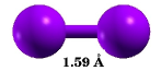
(a) B₂, D_∞h, ${}^{3}\Sigma_{g}^{-}$

(b) B₃, D_3h, ²A${}_{1}^{{}^{\prime}}$

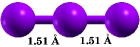
(c) B₃, D_∞h, ${}^{2}\Sigma_{g}^{-}$

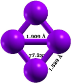
(d) B₄, D_2h, ¹A_g

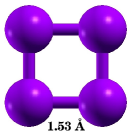
(e) B₄, D_4h, ¹A_1g

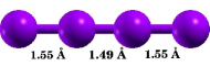
(f) B₄, D_∞h, ${}^{1}\Sigma_{g}^{-}$

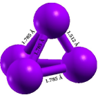
(g) B₄, C_2v, ¹A₁

(h) B₅, C_2v, ²B₂

(i) B₅, C_s, ²A

Figure 3.1: Geometry optimized structures of boron clusters with point group symmetry and the electronic ground state at the configuration interaction level.

The linear photoabsorption spectra of various isomers of the boron clusters were computed using MRSDCI method, as described in subsection 2.1.2.3.

3.2 Results and Discussion

In this section, first we discuss the convergence of our calculations with respect to various approximations and truncation schemes. Thereafter, we present and discuss the results of our calculations for various clusters.

3.2.1 Convergence of Calculations

Here, we carefully examine the convergence of the calculated absorption spectra with respect to the size and quality of the basis set, along with various truncation schemes in the CI calculations.

3.2.1.1 Choice of the basis set

In general, the results of electronic structure calculations depend upon the quality and the size of the basis set employed. While several contracted Gaussian basis functions have been devised which can deliver high-quality results on various quantities such as the total energy, correlation energy, and the static polarizabilities of molecules, to the best of our knowledge the basis set dependence of linear optical absorption has not been explored. Since boron shows strong covalent bondings, the basis set used for calculations should have diffuse Gaussian contractions. Therefore, to explore the basis set dependence of computed spectra, we used several basis sets^{123, 124} to compute the optical absorption spectrum of the smallest cluster, i.e., B₂. For the purpose, we used correlation-consistent basis sets named AUG-CC-PVTZ, DAUG-CC-PVDZ, AUG-CC-PVDZ, CC-PVDZ, and DZP, which consist of polarization functions along with diffuse exponents, and were designed specifically for post Hartree-Fock correlation calculations^{123, 124}. From the calculated spectra presented in Fig. 3.2 the following trends emerge: the spectra computed by various augmented basis sets (AUG-CC-PVTZ, DAUG-CC-PVDZ, AUG-CC-PVDZ) are in good agreement with each other in the energy range up to 8 eV, while those obtained using the nonaugmented sets (CC-PVDZ and DZP) disagree with them substantially, particularly in the higher energy range. Given the fact that augmented basis sets are considered superior for molecular calculations, we decided to perform calculations on the all the clusters using the AUG-CC-PVDZ basis set. This is the smallest of the augmented basis sets considered by us, and, therefore, does not cause excessive computational burden when used for larger clusters.

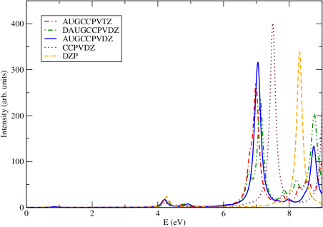
Figure 3.2: Optical absorption in B₂ calculated using various Gaussian contracted basis sets. Increasing more and more diffuse d type Gaussians shows negligible effect on optical spectra.

3.2.1.2 Orbital Truncation Schemes

If the total number of orbitals used in a CI expansion is $N$, the number of configurations in the calculation proliferates as $\approx N^{6}$, which can become intractable for large values of $N$. Therefore, it is very important to reduce the number of orbitals used in the CI calculations. The occupied orbitals are reduced by employing the so-called “frozen-core approximation” described earlier, while the unoccupied (virtual) set is reduced by removing very high-energy orbitals.

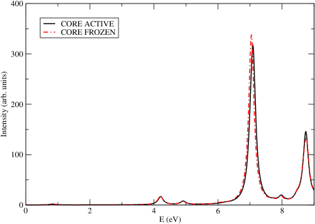
Figure 3.3: The effect of freezing the core orbitals ($1s$) of boron atoms on optical absorption spectrum of B₂. It renders almost no effect on optical absorption spectrum.

The influence of freezing the $1s$ core orbitals on the optical absorption spectrum of B₂ cluster is displayed in Fig. 3.3, from which it is obvious that it makes virtually no difference to the results whether or not the core orbitals are frozen. The effect of removing the high-energy virtual orbitals on the absorption spectrum of B₂ is examined in Fig. 3.4. From the figure it is obvious that if all the orbitals above the energy of 1 Hartree are removed, the absorption spectrum stays unaffected. Therefore, in rest of the calculations, wherever needed, orbitals above this energy cutoff were removed from the list of active orbitals. Theoretically speaking this cutoff is sound, because we are looking for absorption features in the energy range much smaller than 1 Hartree.

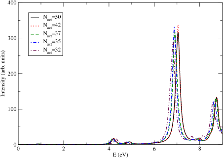
Figure 3.4: The effect of the number of active orbitals (N_act) on the optical absorption spectrum of B₂. Until N_act=42, the optical spectrum does not exhibit any significant change. It corresponds to 1.0 Hartree ($\approx 27.2$ eV) virtual orbital energy.

3.2.1.3 Size of the CI expansion

As mentioned earlier that the electron correlation effects in both the ground and the excited states were accounted in our calculations by including the relevant configurations in the reference list of the MRSDCI expansion. The greater numerical accuracy demands the inclusion of a large number of configurations in the reference list, but that leads to a rapid growth in the size of the CI expansion, making the calculations numerically prohibitive. However, here we are interested in computing the energy differences rather than the absolute energies of various states, for which good accuracy can be achieved even with moderately large CI expansions. In Table 3.1 we present the average number of reference states (N_ref) included in the MRSDCI expansion and average number of configurations (N_total) for different isomers. For a given isomer, the average has been calculated across different irreducible representations which were needed in these symmetry adapted calculations in order to compute the ground and various excited states. The extensiveness of our calculations can be seen from the number N_total, which is $\approx$ 77000 for the simplest cluster, and around four million for each symmetry subspace of B₅. This makes us believe that our results are fairly accurate.

Before we discuss the absorption spectrum for each isomer, we present the ground state energies along with the relative energies of each isomer are given in Table 3.1. The MRSDCI energy convergence threshold was 10^-5 for all the isomers, with 10^-4 as convergence threshold for configuration coefficients. From the results it is obvious that as far as the energetics are concerned, for the B₃ the triangular structure is most stable, while for B₄ and B₅ the rhombus and pentagonal structures, respectively, are favorable.

Table 3.1: The average number of reference configurations (N_ref), and average number of total configurations (N_total) involved in MRSDCI calculations, ground state (GS) energies (in Hartree) at the MRSDCI level, relative energies and correlation energies (in eV) of various isomers of boron clusters.

Cluster	Isomer	Nref	Ntotal	GS energy	Relative
				(Ha)	energy (eV)
B2	Linear	24	77245	-49.27844	0.0
B3	Triangular	36	596798	-73.98998	0.00
	Linear	41	671334	-73.92906	1.66
B4	Rhombus	37	1127918	-98.74004	0.00
	Square	40	1070380	-98.73785	0.06
	Linear	34	1232803	-98.66575	2.02
	Distorted Tetrahedron	28	1253346	-98.63213	2.94
B5	Pentagon	22	3936612	-123.42652	0.00
	Distorted Tri. bipyramid1	7	3927508	-123.31485	3.04

• C_s symmetry of isomer converted to C₁ in calculations.

3.2.2 MRSDCI Photoabsorption Spectra of Boron Clusters

Next we present and discuss the results of our photoabsorption calculations for each isomer.

3.2.2.1 B₂

The simplest and most widely studied cluster of boron is B₂ with D_∞h point group symmetry. Using the CISD method, we obtained its optimized bond length to be 1.59 Å (cf. Fig. 3.1LABEL:sub@fig:b2geom), which is in excellent agreement with the experimental value 1.589 Å.¹²⁵. Using a DFT based methodology, Atiş et al.¹¹⁹, obtained a bond length of 1.571 Å, while Howard and Ray calculated it to be 1.61 Å, using the fourth-order perturbation theory (MP4).¹¹⁶

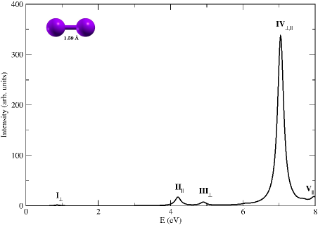
Figure 3.5: The linear optical absorption spectrum of B₂, calculated using the MRSDCI approach. The peaks corresponding to the light polarized along the molecular axis are labeled with the subscript $\parallel$, while those polarized perpendicular to it are denoted by the subscript $\perp$. For plotting the spectrum, a uniform linewidth of 0.1 eV was used.

Because the ground state of B₂ is a spin triplet, its many-particle wavefunction predominantly consists of a configuration with two degenerate Singly Occupied Molecular Orbital (SOMO) referred to as $H_{1}$ and $H_{2}$ in rest of the discussion. The excited state wavefunctions will naturally consist of configurations involving electronic excitations from the occupied MOs to the unoccupied MOs starting from LUMO ($L$ for short). Our calculated photoabsorption spectrum shown in Fig. 3.5 is characterized by weaker absorptions at low energies, and a very intense one at high energy. The many-particle wavefunctions of excited states contributing to various peaks are presented in Table LABEL:Tab:table_b2_lin. A feeble peak appears near 0.85 eV, dominated by $H_{2}\rightarrow L$ and $H_{2}\rightarrow L+4$ excitations compared to the HF reference configuration. It is followed by a couple of smaller peaks at 4.20 and 4.91 eV. The most intense peak is found at 7.05 eV, to which two closely spaced states contribute. Transition to the state near 6.97 eV is polarized transverse to the bond length, while the one close to 7.05 eV carries the bulk of oscillator strength, and is reached by longitudinally polarized photons. All these states exhibit strong mixing of singly-excited configurations. Near 8 eV, a smaller peak appears which has strong contributions from doubly-excited configurations $H-1\rightarrow L$; $H_{1}\rightarrow L+2$ and $H-1\rightarrow L$; $H_{2}\rightarrow L+2$. The wavefunctions of the excited states contributing to all the peaks exhibit strong configuration mixing, instead of being dominated by single configurations, pointing to the plasmonic nature of the optical excitations.¹²⁶

3.2.2.2 B₃

Boron trimer has two possible isomers, triangular and the linear one shown in Figs. 3.1LABEL:sub@fig:b3trgeom and 3.1LABEL:sub@fig:b3lingeom. We found equilateral triangle with D_3h symmetry to be the most stable isomer. The optimized bond length for triangular isomer is 1.55 Å, with the ground state (${}^{2}A_{1}^{{}^{\prime}}$) energy 1.66 eV lower than that of its linear counterpart. We also explored the possibility of isosceles triangular structure as a favorable one, because B₃ is an open-shell system, making it a possible candidate for Jann-Teller distortion. However, the CCSD optimized geometry corresponding to the isosceles structure is so slightly different compared to the equilateral one, that it is unlikely to affect the optical absorption spectrum in a significant manner. Our calculated bond length is in good agreement with experimental value 1.57 Ź⁰⁷, as well as with other reported theoretical values of 1.553 Å,¹¹⁷ 1.56 Å ¹¹⁶ and 1.548 Å.¹¹⁹

The linear B₃ isomer with the D_∞h symmetry, and the ${}^{2}\Sigma_{g}^{-}$ as ground state, was found to have equal bond lengths. Our CISD optimized bond length of 1.51 Å agrees well with the value 1.518 Å reported by Atiş et al.¹¹⁹

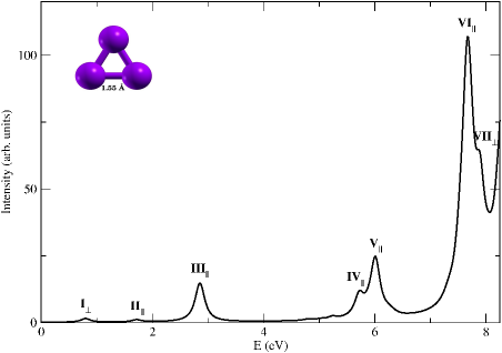
Figure 3.6: The linear optical absorption spectrum of triangular B₃ calculated using the MRSDCI approach. Peaks corresponding to light polarized in the plane of the molecule are labeled with subscript $\parallel$, while those polarized perpendicular to the plane are denoted by the subscript $\perp$. For plotting the spectrum, a uniform linewidth of 0.1 eV was used.

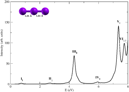
Figure 3.7: The linear optical absorption spectrum of linear B₃, calculated using the MRSDCI approach. The peaks corresponding to the light polarized along the molecular axis are labeled with subscript $\parallel$, while those polarized perpendicular to it are denoted by the subscript $\perp$. For plotting the spectrum, a uniform linewidth of 0.1 eV was used.

The photoabsorption spectra of two isomers of B₃ are presented in Figs. 3.6 and 3.7. The corresponding many-particle wavefunctions of excited states contributing to various peaks are presented in Table LABEL:Tab:table_b3_tri and LABEL:Tab:table_b3_lin. It is obvious that in the linear structure, absorption begins at a lower energy as compared to the triangular one, although the intensity of its low-energy peaks is very small. In the triangular isomer on the other hand, most of the intensity is concentrated at rather high energies, except for a weaker peak close to 3 eV. The optical spectra of linear isomer begins with very weak peaks at 0.7 eV (longitudinal polarization) and 2.7 eV (transverse polarization), with their many-particle wavefunctions dominated by singly-excited configurations. The relatively intense peak at 4.3 eV corresponding to a longitudinally polarized transition, is dominated by doubly-excited configurations. It is followed by a small peak mainly due to single excitation $H-2\rightarrow L$, near 5.9 eV. The most intense peak of the spectrum occurs at 7.4 eV, followed by another strong peak close to 7.7 eV. Both the features correspond to longitudinally polarized transitions, with the many particle wavefunctions of the concerned states being strong mixtures of single and double excitations with respect to the HF reference state. We note that in the absorption spectrum of the linear cluster, quite expectedly, the bulk of the oscillator strength is carried by longitudinally polarized transitions.

Because the triangular cluster is a planar cluster, its orbitals can be classified as in-plane $\sigma$ orbitals, and the out-of-plane $\pi$ orbitals. Both the HOMO (a singly occupied orbital, in this case) and the LUMO for this isomer are $\sigma$-type orbitals. For this system, two types of optical absorptions are possible: (a) those polarized in the plane of the cluster, and (b) the ones polarized perpendicular to that plane. Our calculations reveal that the transitions corresponding to perpendicular polarization ($z$ direction), except for a couple of peaks, have negligible intensities. From Fig. 3.6 it is obvious that the optical absorption in the triangular isomer starts with a very weak $z-$polarized feature near 0.8 eV (peak I), corresponding to a state with the wavefunction dominated by single excitations ($\pi\rightarrow\sigma^{*}$). This is followed by a series of peaks ranging from II to VI which correspond to the photons polarized in the plane of the cluster. All these peaks are dominated by states consisting primarily of singly-excited configurations of the $\sigma\rightarrow\sigma^{*}$ type. The most intense peak VI is followed by a shoulder-like feature (VII) corresponding to a $z$-polarized absorption.

If we compare the absorption spectra of the linear and the triangular B₃, the peak at 4.34 eV in the spectrum of the linear cluster is the distinguishing feature, and can be used to differentiate between the two isomers.

3.2.2.3 B₄

For the B₄ cluster, we investigated the rhombus, square, linear and tetrahedral structures. While the rhombus shaped isomer was found to have the lowest energy, but the square isomer is higher in energy only by a small amount. As a matter of fact, at the HF level the energies of the two isomers were found to be almost degenerate. It was only after the electron correlation effects were included at the CI level that the rhombus stabilized by $\approx$ 0.06 eV (cf. Table 3.1)with respect to the square. For the rhombus, the ground state was ${}^{1}A_{g}$, with the optimized bond length 1.529 Å, and the short diagonal length 1.909 Å. These results are in good agreement with with the corresponding lengths of 1.528 Å and 1.885 Å reported by Boustani,¹¹⁷, and 1.523 Å and 1.884 Å computed by Atiş et al.¹¹⁹ Both HOMO and LUMO of rhombus isomer are $\sigma$ orbitals.

For the square isomer, with D_4h symmetry, the electronic ground state is expectedly ¹A_1g. As shown in Fig. 3.1LABEL:sub@fig:b4sqrgeom, our optimized bound length is 1.53 Å, which agrees well with the values 1.527 Å and 1.518 Å as reported in Refs. ¹¹⁷ and ¹¹⁹. In this isomer, HOMO is a $\sigma$ orbital while LUMO is a $\pi$ orbital.

Linear B₄, with the D_∞h symmetry, has the electronic ground state of ${}^{1}\Sigma_{g}^{-}$. However, energetically linear structure is 2.02 eV higher than the rhombus one (cf. Table 3.1) which rules out its existence at the room temperatures. As per Fig. 3.1LABEL:sub@fig:b4lingeom , the central bond length was found to be 1.49 Å, with the two outer bonds being 1.55 Å in length. For the same bonds, Atiş et al. reported these lengths to be 1.487 Å and 1.568 Å, respectively.¹¹⁹

The distorted tetrahedral structure having C_3v symmetry, made up of four isosceles triangular faces with lengths 1.785 Å, 1.785 Å and 1.512 Å. This isomer also lies much higher in energy as compared to the most stable rhombus structure.

The absorption spectra of rhombus, square, linear, and tetrahedral isomers are presented in Figs. 3.8, 3.9, 3.10, and 3.11 respectively. From the figures it is obvious that the general features of the absorption spectra of rhombus and square isomers are similar, except that the rhombus spectrum, with the onset of the absorption near 4 eV, is red-shifted by about 1 eV as compared to the square. The absorption spectrum of the linear structure is blue-shifted as compared to the rhombus and square shaped isomers, with the majority of absorption occurring in the energy range 5–8 eV. This aspect of the photoabsorption in B₄ is similar to the case of B₃ for which also the linear structure exhibited a red-shifted absorption compared to the triangular one.

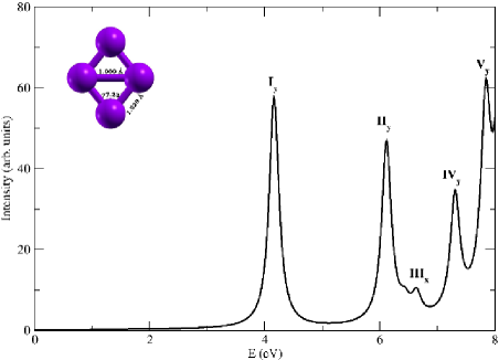
Figure 3.8: The linear optical absorption spectrum of B₄ rhombus geometry using the MRSDCI approach. Isomer is aligned in $x-y$ plane with short diagonal along $x$-axis. Peaks corresponding to light polarized along $x$ and $y$-axis are labeled with subscript $x$ and $y$. For plotting the spectrum, a uniform linewidth of 0.1 eV was used.

Since B₄ rhombus isomer has $D_{2h}$ symmetry, we can represent the absorption due to light polarized in different directions in terms of irreducible representations of $D_{2h}$. So absorption due to in-plane polarized light corresponds to $B_{1u}$ and $B_{2u}$, while $B_{3u}$ corresponds to light polarized in the direction perpendicular to the plane of the isomer.

The polarization resolved absorption spectrum of rhombus B₄, as shown in Fig. 3.8, exhibits a rather red-shifted nature as compared to the linear isomer. The many-particle wavefunctions of excited states contributing to various peaks are presented in Table LABEL:Tab:table_b4_rho. The onset of spectrum is seen at 4.15 eV followed by a peak at around 6.12 eV. Both of them are due to $y-$polarized component, i.e. along the larger diagonal. The dominant contribution to these peaks come from $\sigma\rightarrow\pi^{*}$ for former, and $\pi\rightarrow\pi^{*}$ for latter. The $x$-component does not contribute much in the whole spectrum, except for minor peaks at 4.2 eV and 6.6 eV. It is characterized by mainly $\pi\rightarrow\pi^{*}$ type transitions. It is followed by a relatively low intensity peak at 7.3 eV due to $y$-polarized component with leading contribution from $\sigma\rightarrow\pi^{*}$ transitions. The most intense peak, at 7.84 eV, having $y$-polarization component, is characterized by $\sigma\rightarrow\pi^{*}$ type of transitions. There are no direct $H\rightarrow L$ transitions for this isomer, because they are dipole forbidden. The absorption due to light polarized in the direction perpendicular to the plane of isomer is negligible.

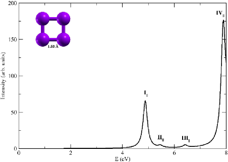
Figure 3.9: The linear optical absorption spectrum of B₄ square geometry using MRSDCI approach. Isomer is aligned in $x-y$ plane. Spectrum represents the equal contribution from light polarized in $x$ and $y$ direction. Peaks corresponding to light polarized in the plane of the molecule are labeled with subscript $\parallel$. For plotting the spectrum, a uniform linewidth of 0.1 eV was used.

The square B₄ isomer, because of its symmetry, gets equal contribution to absorption spectrum from both $x-$ and $y-$component. It corresponds to in-plane polarization due to $B_{1u}$ and $B_{2u}$ irreducible representation, while $B_{3u}$ corresponds to light polarized in the direction perpendicular to the plane of the isomer. However, in this isomer also, the contribution due to latter is quite negligible. The many-particle wavefunctions of excited states contributing to various peaks are presented in Table LABEL:Tab:table_b4_sqr. It shows just one major peak at 4.88 eV below 7 eV, characterized by $\sigma\rightarrow\pi^{*}$;$\sigma\rightarrow\pi^{*}$ double excitation. Two smaller peaks appear in this range at 5.5 eV and 6.4 eV, with leading contributions from $\sigma\rightarrow\pi^{*}$;$\sigma\rightarrow\pi^{*}$ and $\sigma\rightarrow\pi^{*}$;$\pi\rightarrow\pi^{*}$ excitations respectively. Beyond 7 eV, there are many closely spaced peaks including the most intense one at 7.89 eV. It is characterized by double excitation $\sigma\rightarrow\pi^{*}$;$\pi\rightarrow\pi^{*}$. In this isomer also, a direct $H\rightarrow L$ transition is forbidden. Though, there is very little difference in total energies of rhombus and square isomers of B₄, their optical absorption spectra are completely different. They can be easily identified from each other by looking at number of peaks below 7 eV energy. Rhombus exhibits two major peaks, while square has just one.

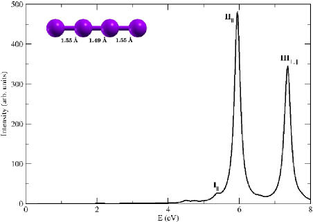
Figure 3.10: The optical absorption spectrum of linear B₄, calculated using the MRSDCI approach. The peaks corresponding to the light polarized along the molecular axis are labeled with subscript $\parallel$, while those polarized perpendicular to it are denoted by the subscript $\perp$. For plotting the spectrum, a uniform linewidth of 0.1 eV was used.

Linear B₄ isomer exhibits absorption with few, but sharp peaks. The many-particle wavefunctions of excited states contributing to various peaks are presented in Table LABEL:Tab:table_b4_lin. The onset of optical absorption occurs near 4.5 eV, due to absorption of long-axis polarized light, followed by two major peaks at 5.95 eV, and 7.36 eV. The first of these two intense peaks, peak II is dominated by singly-excited configurations, while the second one (peak III) is a strong mixture of both singly- and doubly-excited configurations with respect to the HF reference configuration.

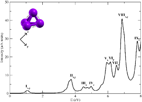
Figure 3.11: The linear optical absorption spectrum of B₄ distorted tetrahedral geometry using the MRSDCI approach. Peaks corresponding to light polarized along $x$, $y$ and $z$-axis are labeled with subscript $x$, $y$ and $z$ respectively. For plotting the spectrum, a uniform linewidth of 0.1 eV was used.

The 3D structure, a distorted tetrahedral isomer, exhibits an absorption spectrum very different from other isomers, as displayed in Fig. 3.11. The many-particle wavefunctions of excited states contributing to various peaks are presented in Table LABEL:Tab:table_b4_tetra. It is the only B₄ isomer to exhibit peaks below 4 eV. The absorption spectrum is spread over a much larger energy range, and is almost continuous. The oscillator strengths associated with various peaks are much smaller than in other isomers, and most of the peaks appear pairwise. The onset of absorption spectrum is seen at around 1.1 eV, characterized mainly by an excited dominated by single-excitation $H\rightarrow L$ (cf. Table LABEL:Tab:table_b4_tetra). In this isomer, in contrast to other B₄ isomers, direct $H\rightarrow L$ transitions are allowed. Higher energy peaks in this isomer are dominated by doubly-excited configurations, and, are, therefore, sensitive to the electron-correlation effects.

3.2.2.4 B₅

We investigated two isomers of B₅: a Jahn-Teller distorted pentagon with the C_2v symmetry, and (b) a triangular bipyramid with the C_s point group symmetry. The latter one is the second 3-D structure of the boron clusters probed in this work. The lowest lying pentagon isomer, has ²B₂ electronic ground state, and is 3.04 eV lower in energy as compared to the bipyramid structure. For the pentagon, the symmetry of ground state at the Self-Consistent Field (SCF) level was A₁, however, at the MRSDCI level the B₂ state became lower in energy, in agreement with the previous calculations of Boustani.¹¹⁷ Our optimized geometry for the pentagon (Fig. 3.1LABEL:sub@fig:b5pengeom) corresponds to an average bond length of 1.56 Å, as against 1.57 Å reported by Boustani¹¹⁷, and 1.644 Å reported by Atiş et al.¹¹⁹. The singly occupied molecular orbital (denoted by $H$) and LUMO of pentagon isomers are of $\pi$ and $\sigma$ type, respectively. The bond lengths for the bipyramid structure are shown in Fig. 3.1LABEL:sub@fig:b5tetgeom, with an average bond length of 1.704 Å. The triangular base was found to be isosceles with 1.97 Å as equal sides, and 1.75 Å as the other side.

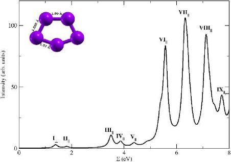
Figure 3.12: The linear photo-absorption spectrum of pentagon B₅, calculated using the MRSDCI approach. The peaks corresponding to the light polarized in the plane of the molecule are labeled with subscript $\parallel$, while those polarized perpendicular to it are denoted by the subscript $\perp$. For plotting the spectrum, a uniform linewidth of 0.1 eV was used.

The absorption spectra of the two isomers are presented in Figs. 3.12 and 3.13. The many-particle wavefunctions of excited states contributing to various peaks are presented in Table LABEL:Tab:table_b5_pen and LABEL:Tab:table_b5_tet respectively. From the figures it is obvious that the intense absorption in the bipyramid starts at much lower energies as compared to the pentagonal isomer. Intense absorption peaks in pentagon B₅ are located at energies higher than 5 eV, with three equally intense peaks at 5.58 eV, 6.30 eV and 7.16 eV, with the photons polarized along the plane of the molecule direction. It has an underlying low intensity absorption contribution from photons polarized along $z-$ direction, which is perpendicular to the molecular plane. The major contribution to the peak at 5.58 eV comes from $\pi\rightarrow\sigma^{*}$ and $\sigma\rightarrow\sigma^{*}$, single excitations. The latter configuration also contributes to the most intense peak at 6.30 eV. The peak at 7.16 eV is mainly due to $\sigma\rightarrow\sigma^{*}$ type transitions.

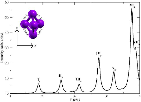
Figure 3.13: The linear photo-absorption spectrum of distorted triangular bipyramid B₅, calculated using the MRSDCI approach. Peaks corresponding to light polarized along $x$, $y$ and $z$-axis are labeled with subscript $x$, $y$ and $z$ respectively. For plotting the spectrum, a uniform linewidth of 0.1 eV was used.

Since the B₅ triagonal bipyramid isomer is not a symmetric one, the calculations were done using C₁ symmetry, thereby increasing the difficulty in diagonalizing the Hamiltonian. Hence, in order to reduce the matrix size, we have used a smaller number of reference configurations, and also relaxed the energy convergence threshold criterion a little.

The optical absorption spectrum of B₅ triangular bipyramid isomer is exhibited by almost equally spaced peaks at relatively lower energies. The optical absorption starts at 1.74 eV characterized by $H-1\rightarrow L+4$ configuration. It is followed by two equal intensity peaks at 3.16 eV and 4.27 eV with contributions from single excitations $H-2\rightarrow H\mbox{ and }H-1\rightarrow L+2$, respectively. The most intense peak is found at 7.52 eV dominated by the doubly excited configuration $H-2\rightarrow H\>;\>H-1\rightarrow L+2$. There are two distinguishing features as far as the optical absorption in the two isomers is concerned: (a) presence of three intense peaks in the higher energy region of the absorption spectrum of the pentagonal isomer, and (b) occurrence of equally spaced absorption peaks at lower energies in the spectrum of bipyramidal isomer.

3.3 Summary

We presented systematic large-scale all-electron correlated calculations of photoabsorption spectra of boron clusters B_n, ($n=$2–5) with several possible isomers of each cluster. The calculations were performed using the MRSDCI method which takes electron correlations into account at a sophisticated level, both for the ground and the excited states. For a cluster consisting of a given number of atoms, significant changes were observed in absorption spectra for different isomers, indicating a strong structure-property relationship. Therefore, our computed spectra can be used in the future photoabsorption experiments to distinguish between different isomers of a cluster, something which is not possible with the conventional mass spectrometry. We also analyzed the many-particle wavefunctions of various excited states and found them to be a mixture of a large number of configurations, indicating the nature of photoexcited states in these clusters to be plasmonic.¹²⁶ A noteworthy aspect of the ground state photoabsorption of various clusters was the absence of high-intensity peaks in the low-energy region of the spectrum. The most intense peaks occurred at higher energies involving orbitals away from the Fermi level, consistent with the fact that the bulk boron is an indirect bandgap semiconductor, with no optical absorption at the gap. In other words, optical absorption features of bulk boron were already evident in smaller clusters.

Chapter 4 Theory of Linear Optical Absorption in Various Isomers of Boron Clusters B₆ and B${}_{6}^{+}$

This chapter is based on a published paper, Eur. Phys. J. D, 67, 98 (2013)
by Ravindra Shinde and Alok Shukla.

Boron clusters exhibit a number of interesting properties, comparable only to its neighbor, carbon. The study of smaller boron clusters has unraveled a great potential for applications in nanotechnology. For example, some planar boron structures are also found to be analogous to hydrocarbons ¹¹. The all-boron clusters are found promising candidates as inorganic ligands ^{62, 63}. A circular B${}_{19}^{-}$ cluster, with a unit of B₆ wheel in the center behaves as a Wankel motor, i.e. the inner B₆ wheel rotating opposite to the outer B₁₃ ring ^{127, 128}. As far as optical properties of boron clusters are concerned, only a small number of reports available. Marques and Botti studied the optical absorption spectra of B₂₀, B₃₈, B₄₄, B₈₀ and B₉₂ using time-dependent DFT ¹²¹. To the best of our knowledge, no other experimental results are available on the optical absorption of boron clusters.

In the previous chapter, we studied the optical absorption in boron clusters B_n (n=2 – 5) using a large-scale multi-reference configuration interaction method ¹²⁹. This method is quite expensive and scales as N⁶, where N is the number of orbitals used in the calculations, it becomes more and more computationally demanding for large clusters, or clusters with no symmetry. However good insights can be achieved with much less expensive method known as CIS, containing only one electron excitations from the Hartree-Fock ground state ⁸⁵. This method has been extensively used for the study of the excited states and optical absorption in various other systems ^{130, 131, 132, 133, 134, 135}. Since optical absorption spectra is very sensitive to the structural geometry, the optical absorption spectroscopy along with the extensive calculations of optical absorption spectra, can be used to distinguish between distinct isomers of a cluster. In this report, we present extensive calculations of the linear optical absorption spectrum of low-lying isomers of B₆ and B${}_{6}^{+}$ clusters with different structures. This study, along with the experimental absorption spectra, can lead to identification of these distinct isomers. Also, in the interpretation of the measured spectra, the theoretical understanding of the excited states of clusters plays an important role ¹³⁶.

The remainder of this chapter is organized as follows. Next section describes the theoretical and computational details of the work, followed by section 4.2, in which results are presented and discussed. In the last section we summarize our findings. A Detailed information regarding the excited states contributing to the optical absorption is presented in the Appendix B.

4.1 Theoretical and Computational Details

Different possible arrangements and orientations of atoms of the B₆ cluster (both neutral and cationic) were randomly selected for the initial configurational search of geometries of isomers. For a given spin multiplicity, the geometry optimization was done at a correlated level, i.e., at the CCSD level ¹³⁷ with 6-311G(d,p) basis set as implemented in gaussian09¹³⁸. Since neutral cluster can have singlet or higher spin multiplicity, the optimization was repeated for different spin configurations to get the lowest energy isomer. Similarly for cationic clusters with odd number of electrons, spin multiplicities of 2 and 4 were considered in the optimization. In total, we have obtained 11 neutral B₆ and 8 cationic B${}_{6}^{+}$ low-lying isomers. These optimized geometries of neutral B₆ cluster, as shown in Fig. 4.1, are found to be in good agreement with other available reports. Figure 4.15 shows the corresponding geometries of cationic B${}_{6}^{+}$ cluster. The unique bond lengths, point group symmetry and the electronic ground states are given in respective sub-figures.

The excited state energies of isomers are obtained using the ab initio CIS approach. In this method, different configurations are constructed by promoting an electron from an occupied orbital to a virtual orbital. For open-shell systems, we have used unrestricted Hartree-Fock formalism for constructing CIS configurations. Excited states of the system will have a linear combination of all such substituted configurations, with corresponding variational coefficients. The energies of the excited states will then be obtained by diagonalizing the Hamiltonian in this configurational space ⁸⁶. The dipole matrix elements are calculated using the ground state and the excited state wavefunctions. This is subsequently used for calculating the optical absorption cross section assuming Lorentzian lineshape, with some artificial finite linewidth.

EOM-CCSD calculations were done on few representative clusters in order to justify the use of CIS method for optical absorption calculations ^{92, 139}. Details are discussed in the next section. The contribution of wavefunction of the excited states to the absorption peaks as well as an analysis based on natural transition orbitals gives an insight into the nature of optical excitation.

As discussed in the chapter 3, we have extensively studied the dependence of basis sets, freezing of 1s² chemical core on the computed photoabsorption spectra of neutral boron clusters ¹²⁹. We have shown that the optical absorption spectra of small boron clusters do not change even if we freeze the chemical core of boron atoms. Therefore, in all these calculations $1s^{2}$ chemical core of each boron atom has been frozen.

4.2 Results and Discussion

In this section, we discuss the structure and energetics of various isomers of neutral and cationic B₆ cluster, followed by discussion of results of computed absorption spectra and nature of photo-excitations.

In the many-particle wavefunction analysis of excited states contributing to the various peaks , we have used following convention. For doublet systems $H_{1\alpha}$ denotes the singly occupied molecular orbital. For triplet systems, two SOMOs are denoted by $H_{1\alpha}$ and $H_{2\alpha}$, while $H$ and $L$ stands for highest occupied molecular orbital and lowest unoccupied molecular orbital respectively. For quartets, the third singly occupied molecular orbital is denoted by $H_{3\alpha}$.

4.2.1 B₆

We have found a total of 11 isomers of neutral B₆ cluster with stable geometries as shown in the Fig. 4.1. ¹⁴⁰ The relative standings in energy are presented in the Table 4.1, along with point group symmetries and electronic states.

Table 4.1: Point group, electronic state, total energies and values of $\langle S^{2}\rangle$ before and after ($\langle S^{2}_{a}\rangle$) spin annihilation operation for different isomers of of B₆ cluster.

Sr.	Isomer	Point	Elect.	Total	$\langle S^{2}\rangle$	$\langle S^{2}_{a}\rangle$
no.		group	State	Energy (Ha)
1	Planar ring (triplet)	C2h	${}^{3}A_{u}$	-147.795051	2.720	2.180
2	Incomplete wheel	C2v	${}^{3}B_{1}$	-147.774166	2.750	2.217
3	Bulged wheel	C5v	${}^{1}A_{1}$	-147.764477	0.000	0.000
4	Planar ring (singlet)	Cs	${}^{1}A^{{}^{\prime}}$	-147.720277	0.000	0.000
5	Octahedron	Oh	${}^{3}A_{1g}$	-147.678302	2.082	2.003
6	Threaded tetramer	C1	${}^{3}A$	-147.676776	2.019	2.000
7	Threaded trimer	C2v	${}^{3}B_{1}$	-147.667709	2.087	2.001
8	Twisted trimers	C1	${}^{1}A$	-147.645847	0.000	0.000
9	Planar trimers	D2h	${}^{1}A_{g}$	-147.645522	0.000	0.000
10	Convex bowl	C1	${}^{1}A$	-147.612607	0.000	0.000
11	Linear	D∞h	${}^{1}\Sigma_{g}$	-147.449013	0.000	0.000

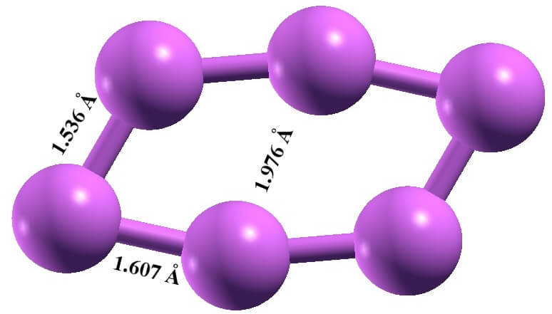
(a) C_2h, ${}^{3}A_{u}$
Planar ring (Tp)

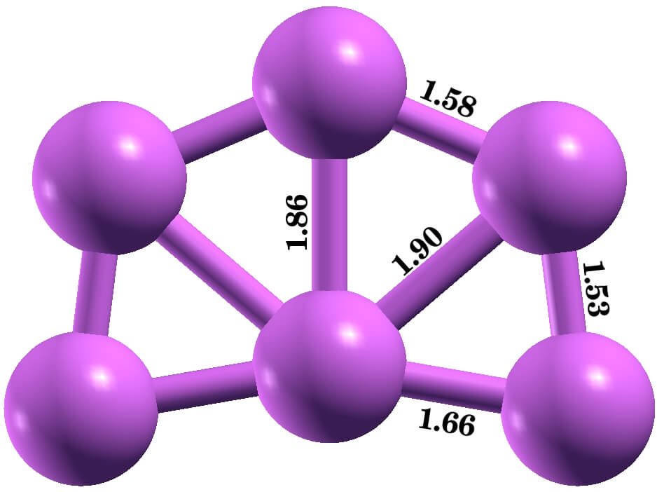
(b) C_2v, ${}^{3}B_{1}$
Incomplete Wheel

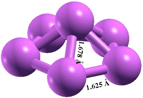
(c) C_5v, ${}^{1}A_{1}$ Bulged wheel

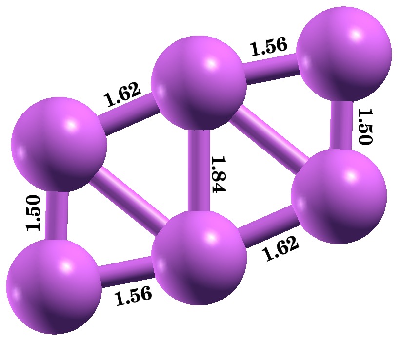
(d) C_s, ${}^{1}A^{{}^{\prime}}$
Planar ring (Sg)

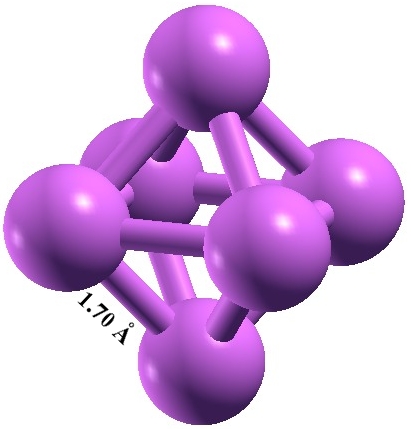
(e) O_h, ${}^{3}A_{1g}$ Octahedron

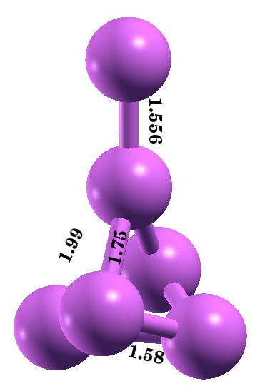
(f) C₁, ${}^{3}A$ Threaded tetramer

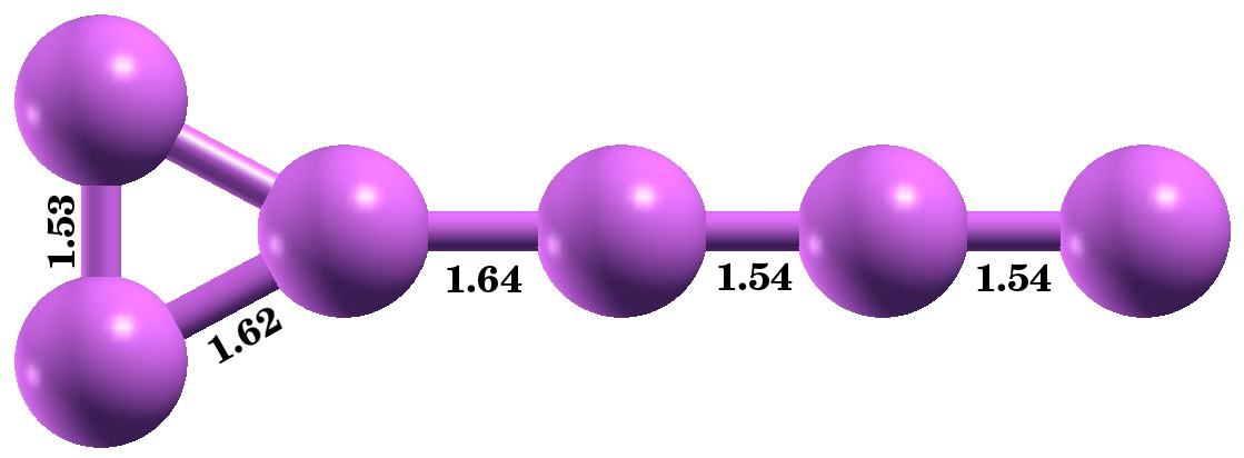
(g) C_2v, ${}^{3}B_{1}$ Threaded trimer

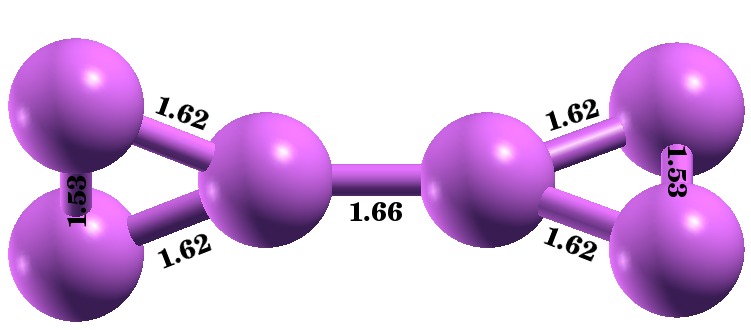
(h) C₁, ${}^{1}A$
Twisted trimers

(i) D_2h, ${}^{1}A_{g}$ Planar trimers

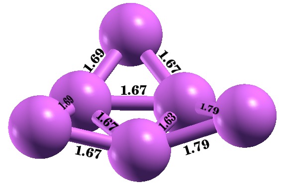
(j) C₁, ${}^{1}A$ Convex bowl

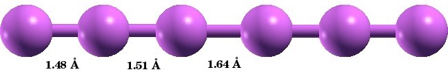
(k) D_∞h, ${}^{1}\Sigma_{g}$ Linear

Figure 4.1: Geometry optimized ground state structures of different isomers of neutral B₆ clusters, along with the point group symmetries obtained at the CCSD level.

The most stable isomer of B₆ cluster has ring-like planar structure, with C_2h point group symmetry. Although B₆ has an even number of electrons, the electronic ground state of this isomer is a triplet – an open shell system. The equilibrium geometry obtained in our calculation is in good agreement with the recently reported values.^{119, 141, 142, 143} The optical absorption spectrum calculated using the CIS approach is as shown in the Fig. 4.2. It is mainly characterized by feeble absorption in the visible range, but much stronger absorption at higher energies. The many particle wave-functions of excited states contributing to various peaks are presented in Table LABEL:Tab:table-neutral-planar-ring-triplet. The first absorption peak at 2.85 eV with very low intensity is characterized by $H_{\alpha}-2\rightarrow L_{\alpha}$ and $H_{1\alpha}\rightarrow L_{\alpha}$ transitions. The natural transition orbital analysis of the peak at 3.42 eV shows that this is dominated by a $\pi\rightarrow\pi^{*}$ transition. Due to planar nature of the isomer, we can classify the absorption into two categories: (a) those with polarization along the direction of the plane and (b) polarization perpendicular to the plane. In this case, it is seen that, in most of the cases, the absorption is due to polarizations along the plane of the isomer. Also, instead of being dominated by single configurations, the wavefunctions of the excited states contributing to all the peaks exhibit strong configuration mixing. This is an indicator of plasmonic nature of the optical excitations.¹²⁶

The optical absorption spectrum for the same isomer is calculated using a sophisticated EOM-CCSD method, as shown in Fig. 4.3. A complete one-to-one mapping of configurations involved in excited states of CIS and EOM-CCSD calculations is observed, along with some double excitations with minor contribution. The spectrum of EOM-CCSD is red-shifted, as expected, because this method takes electron correlations into account at a high level.

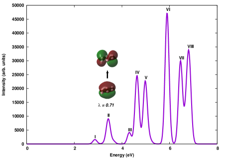
Figure 4.2: The linear optical absorption spectrum of planar ring (triplet) B₆ isomer, calculated using the CIS approach, along with the natural transition orbitals involved in the excited states corresponding to the peak II (3.42 eV). Parameter $\lambda$ refers to a fraction of the NTO pair contribution to a given electronic excitation.

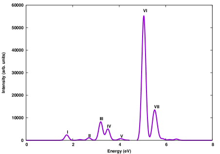
Figure 4.3: The linear optical absorption spectrum of planar ring (triplet) B₆ isomer, calculated using the EOM-CCSD approach.

The second low lying isomer of B₆ is another planar structure resembling an incomplete wheel, i.e. one outer atom removed from B₇ wheel cluster. This isomer is also a triplet system with C_2v symmetry, lying 0.56 eV above the global minimum structure. The optimized geometry is in good agreement with the other previously available reports ^{142, 144}. This is one of the isomers showing feeble optical absorption at lower energies (cf. Fig. 4.4). The many particle wave-functions of excited states contributing to various peaks are presented in Table LABEL:Tab:table-neutral-incomplete-wheel. Degenerate $\pi$ orbitals are involved in the excitations at peak I and II as evident from the NTOs shown in Fig. 4.4.

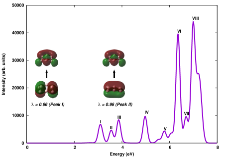
Figure 4.4: The linear optical absorption spectrum of incomplete-wheel B₆ isomer, calculated using the CIS approach, along with the natural transition orbitals involved in the excited states corresponding to the peaks I (3.09 eV) and II (3.55 eV) respectively. Parameter $\lambda$ refers to a fraction of the NTO pair contribution to a given electronic excitation.

A wheel kind of structure, with its center slightly bulged out, is found to be the next stable isomer of B₆. A singlet system with C_5v point group symmetry, lies just 0.83 eV above in energy as compared to the most stable isomer. The pentagonal base has bond length of 1.625 Å and the vertex atom is 1.678 Å away from the corners of the pentagon. Other reported values for those bond lengths are 1.61 Å, 1.66 Å ^{119, 144} and 1.61 Å, 1.659 Å ^{141, 142} respectively. The optical absorption spectrum calculated using CIS approach is presented in Fig. 4.5. The many-particle wavefunctions of excited states contributing to various peaks are presented in Table LABEL:Tab:table-neutral-bulged-wheel. The onset of the spectrum occurs near 3.76 eV, with polarization in the plane of the pentagonal base, characterized by excitations $H-1\rightarrow L+6$ and $H\rightarrow L+6$ with equal contribution.

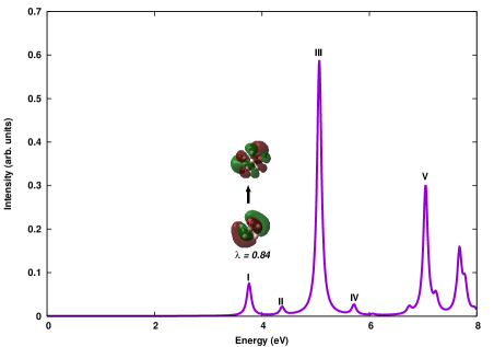
Figure 4.5: The linear optical absorption spectrum of bulged-wheel B₆ isomer, calculated using the CIS approach, along with the natural transition orbitals involved in the excited states corresponding to the peak I (3.76 eV). Parameter $\lambda$ refers to a fraction of the NTO pair contribution to a given electronic excitation.

The spectrum of this singlet isomer is calculated again using EOM-CCSD approach to investigate any involvement of double excitation. The spectrum appears to be red-shifted but the configurations contributing to the excited states corresponding to the peaks of the spectrum are the same as observed in the case of CIS. This makes us confident to use CIS method only to investigate optical absorption spectrum of other isomers.

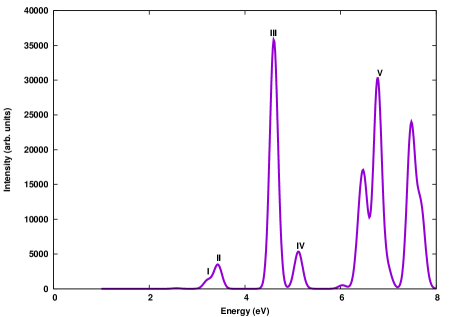
Figure 4.6: The linear optical absorption spectrum of bulged-wheel B₆ isomer, calculated using the EOM-CCSD approach.

A planar ring like structure, resembling the global minimum one; however, with singlet state and C_s symmetry, is the next low lying isomer of B₆ cluster. The optimized geometry is in good agreement with Ref. ¹⁴⁴. The absorption spectrum is presented in Fig. 4.7 and corresponding many-particle wavefunctions of various excited states are presented in Table LABEL:Tab:table-neutral-planar-ring-singlet. The absorption onset occurs at 3.1 eV, characterized by delocalized orbitals with $H-1\rightarrow L$ and $H\rightarrow L+23$ configurations.

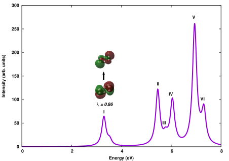
Figure 4.7: The linear optical absorption spectrum of planar-ring B₆ isomer, calculated using the CIS approach, along with the natural transition orbitals involved in the excited states corresponding to the peak I (3.13 eV). Parameter $\lambda$ refers to a fraction of the NTO pair contribution to a given electronic excitation.

An octahedron structure with O_h point group symmetry is the next stable isomer of neutral B₆. Each side of the octahedron is found to be 1.7 Å as compared to the 1.68 Å reported by Atiş et al.¹¹⁹ and Jun et al.¹⁴⁴ The many-particle wavefunctions of the excited states corresponding to various peaks (cf. Fig. 4.8) are presented in Table LABEL:Tab:table-neutral-octahedron. A very feeble absorption at 0.92 eV opens the spectrum, mainly characterized by excitations $H_{1\alpha}\rightarrow L_{\alpha}$ and $H_{2\alpha}\rightarrow L_{\alpha}+1$ with equal contribution. The transition orbitals corresponding to peaks at 0.92 eV and 2.50 eV are as shown in Fig. 4.8.

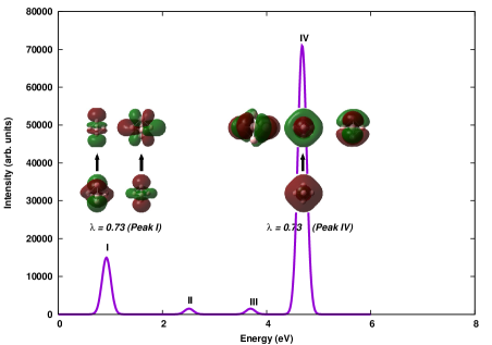
Figure 4.8: The linear optical absorption spectrum of octahedron B₆ isomer, calculated using the CIS approach, along with the natural transition orbitals involved in the excited states corresponding to the peaks I (0.92 eV) and IV (4.68 eV) respectively. Parameter $\lambda$ refers to a fraction of the NTO pair contribution to a given electronic excitation.

Next isomer is previously unreported, with structure of a saddle threaded with dimer from top. It lies just 0.04 eV above the previous octahedron isomer. However the optical absorption spectrum (cf. Fig. 4.9) is completely different. A narrow energy range hosts all the peaks. The onset of intense absorption occurs near 3.06 eV, with major contribution from H${}_{2\alpha}\rightarrow L_{\alpha}+2$ (cf. Table LABEL:Tab:table-neutral-threaded-tetramer). The NTO analysis shows that excitation occurs from the tail end to the saddle section of the isomer.

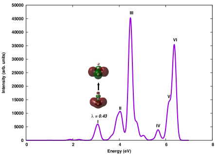
Figure 4.9: The linear optical absorption spectrum of threaded-tetramer B₆ isomer, calculated using the CIS approach, along with the natural transition orbitals involved in the excited states corresponding to the peak I (3.06 eV). Parameter $\lambda$ refers to a fraction of the NTO pair contribution to a given electronic excitation.

An isosceles triangle connected to a linear chain of boron atoms forms the next isomer. This structure with C_2v symmetry and a triplet electronic state has been reported in Ref. ¹⁴⁴, which is in close agreement with our results. The optical absorption spectrum (cf. Fig. 4.10) has distinctive closely lying peaks at 4.03 eV and 4.73 eV. The many-particle wavefunctions of excited states corresponding to various peaks are presented in Table LABEL:Tab:table-neutral-threaded-trimer. As evident from the NTOs involved in transitions at peak I, the electrons tend to be localized at the triangular end of the isomer.

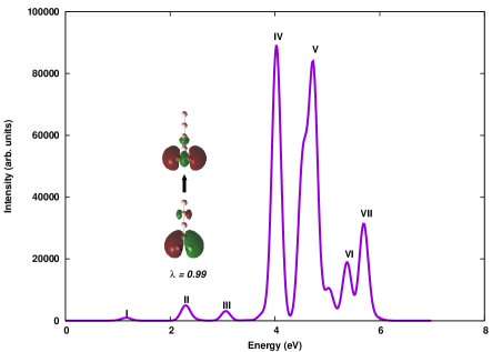
Figure 4.10: The linear optical absorption spectrum of threaded-trimer B₆ isomer, calculated using the CIS approach, along with the natural transition orbitals involved in the excited states corresponding to the peak II (2.28 eV). Parameter $\lambda$ refers to a fraction of the NTO pair contribution to a given electronic excitation.

A structure with two out of plane isosceles triangles joined together is found to be one of the isomers. The geometry has isosceles triangle with lengths 1.62 Å, 1.62 Å and 1.53 Å, while two such triangles are joined by a bond of length 1.66 Å. The respective numbers reported by Ref. ¹⁴⁴ are 1.60 Å, 1.60 Å, 1.50 Å and 1.647 Å respectively. The optical absorption spectrum contains many low intensity peaks except for strongest one at 5.87 eV, as presented in Fig. 4.11. A $\pi\rightarrow\pi^{*}$ transition is observed at 2.22 eV. (cf. Table LABEL:Tab:table-neutral-twisted-trimers).

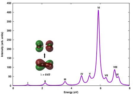
Figure 4.11: The linear optical absorption spectrum of twisted trimers B₆ isomer, calculated using the CIS approach, along with the natural transition orbitals involved in the excited states corresponding to the peak I (2.22 eV). Parameter $\lambda$ refers to a fraction of the NTO pair contribution to a given electronic excitation.

An almost degenerate structure forms the next isomer, lying just 0.009 eV above the previous isomer. Contrary to the previous one, this geometry is completely planar and is a triplet system, with C_2v point group symmetry. Probably because of such a strong near-degeneracy, this isomer has not been reported in the literature before. The many-particle wavefunctions of the excited states corresponding to various peaks (cf. Fig. 4.12) are presented in Table LABEL:Tab:table-neutral-planar-trimers. The spectrum opens with feeble peak. First major peak at 4.69 eV is characterized by $\pi\rightarrow\pi^{*}$ transition, as is evident from the natural transition orbital analysis. First four peaks in the absorption spectra of this isomer are identical to that of twisted trimers isomer. The effect of twisting has effect only on the high energy excitations.

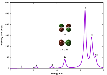
Figure 4.12: The linear optical absorption spectrum of planar trimers B₆ isomer, calculated using the CIS approach, along with the natural transition orbitals involved in the excited states corresponding to the peak IV (4.69 eV). Parameter $\lambda$ refers to a fraction of the NTO pair contribution to a given electronic excitation.

Convex bowl shaped isomer and a perfect linear chain are found very high in energy, ruling out their existence at room temperature. The optical spectra are presented in Figs. 4.13 and 4.14 respectively. The corresponding many-particle wavefunctions of excited states of various peaks are presented in Table LABEL:Tab:table-neutral-convex-bowl and LABEL:Tab:table-neutral-linear. Peak at 2.43 eV in the absorption spectrum of convex bowl isomer shows partially delocalized to fully delocalized nature of transition. The bulk of the oscillator strength of the spectrum of linear isomer is carried by $H-1\rightarrow L+3$ and $H\rightarrow L+2$ having equal contributions. The NTOs corresponding to the excitations involved in the spectrum are shown in Fig. 4.14.

Figure 4.13: The linear optical absorption spectrum of convex-bowl B₆ isomer, calculated using the CIS approach, along with the natural transition orbitals involved in the excited states corresponding to the peaks III (2.43 eV) and IV (2.88 eV) respectively. Parameter $\lambda$ refers to a fraction of the NTO pair contribution to a given electronic excitation.

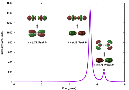
Figure 4.14: The linear optical absorption spectrum of linear B₆ isomer, calculated using the CIS approach, along with the natural transition orbitals involved in the excited states corresponding to the peaks I (5.51 eV) and II (6.51 eV) respectively. Parameter $\lambda$ refers to a fraction of the NTO pair contribution to a given electronic excitation.

4.2.2 B${}_{6}^{+}$

We have found a total of 8 isomers of cationic (B${}_{6}^{+}$) cluster with stable geometries as shown in the Fig. 4.15. The relative standings in energy are presented in the Table 4.2, along with point group symmetries, electronic states and expectation value of $S^{2}$ operator. Since this is a case of an open-shell system, the spin contamination may induce large errors in he computed absorption spectra. We have reported $\langle S^{2}\rangle$ values for excited states corresponding to each peak in the spectra. In most of the cases the geometry of the neutral isomer is retained, reflected in the fact that some peaks show up in the optical absorption spectra at the same energies as those in the neutral cluster.

Table 4.2: Point group, electronic state, total energies and values of $\langle$ S² $\rangle$ before and after spin annihilation operation for different isomers of B${}_{6}^{+}$ cluster.

Sr.	Isomer	Point	Elect.	Total	$\langle$ S2 $\rangle$	$\langle$ S${}^{2}_{a}$ $\rangle$
no.		group	State	Energy (Ha)
1	Planar ring (I)	Cs	${}^{2}A^{{}^{\prime\prime}}$	-147.492831	0.8410	0.7524
2	Bulged wheel	C1	${}^{2}A$	-147.491994	1.0450	0.7909
3	Planar ring (II)	D2h	${}^{2}A_{g}$	-147.480796	0.8503	0.7531
4	Incomplete wheel	C2v	${}^{4}A_{2}$	-147.454234	4.6090	3.9490
5	Threaded trimer	C2v	${}^{4}A_{2}$	-147.429627	3.7671	3.7501
6	Tetra. bipyramid	D4h	${}^{2}B_{1g}$	-147.413145	1.2565	0.8742
7	Linear	D∞h	${}^{4}\Sigma_{u}$	-147.392263	4.8354	4.0712
8	Planar trimers	D2h	${}^{2}B_{2g}$	-147.358494	1.0000	0.7808

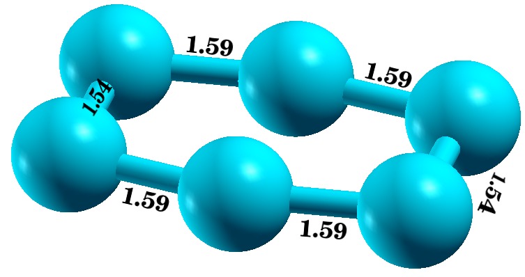
(a) C_s, ${}^{2}A^{{}^{\prime\prime}}$
Planar ring (I)

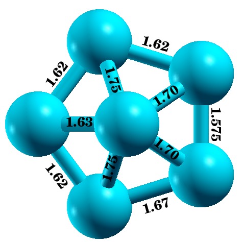
(b) C₁, ${}^{2}A$
Bulged wheel

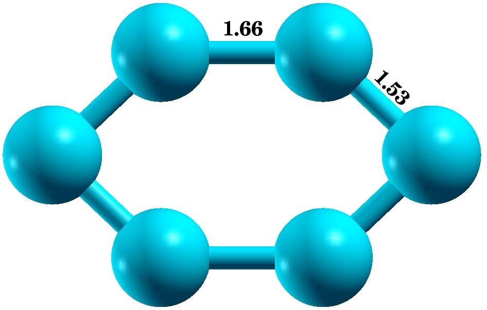
(c) D_2h, ${}^{2}A_{g}$
Planar ring (II)

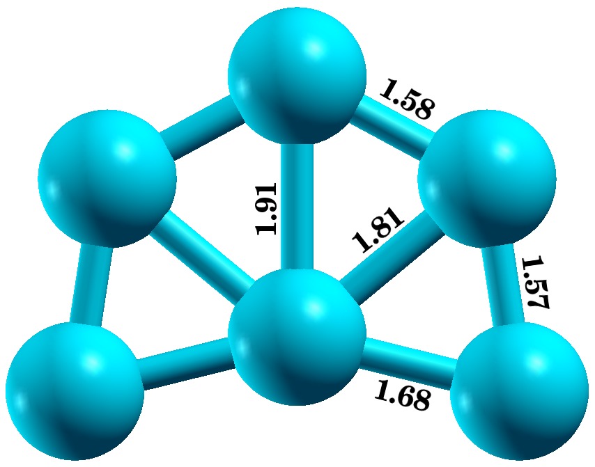
(d) C_2v, ${}^{4}A_{2}$
Incomplete wheel

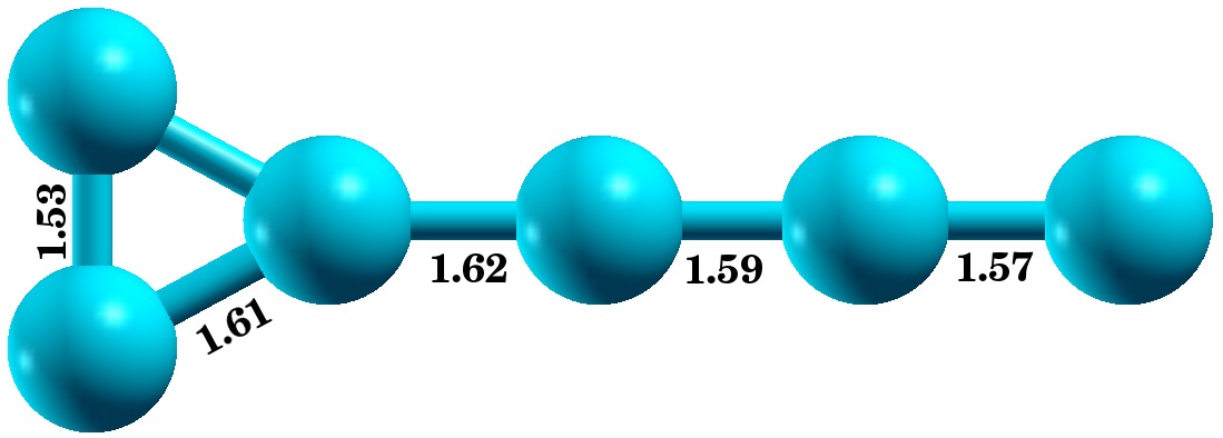
(e) C_2v, ${}^{4}A_{2}$ Threaded trimer

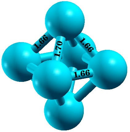
(f) D_4h, ${}^{2}B_{1g}$ Bipyramid

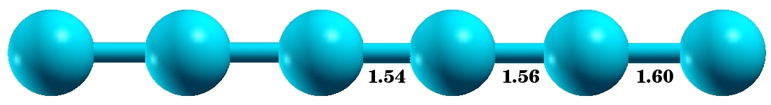
(g) D_∞h, ${}^{4}\Sigma_{u}$ Linear

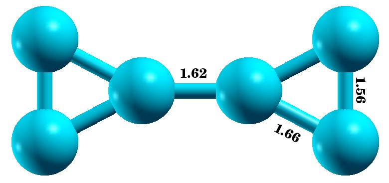
(h) D_2h, ${}^{2}B_{2g}$ Planar trimers

Figure 4.15: Geometry optimized ground state structures of different isomers of cationic B${}_{6}^{+}$ clusters, along with the point group symmetries obtained at the CCSD level.

The most stable isomer of B${}_{6}^{+}$ cluster is a planar ring-type of structure, with C_s point group symmetry. This is in contrast to the other reported geometries which have D_2h symmetry ^{142, 143, 144}. A slight difference in the orientation makes it less symmetric. However, the bonds lengths obtained are in good agreement with those with D_2h symmetric geometry cited above. The optical absorption spectrum calculated using CIS approach is as shown in the Fig. 4.16 and corresponding many-particle wavefunctions of excited states contributing to the various peaks are presented in Table LABEL:Tab:table-cationic-planar-ring. Similar to the neutral counterpart, this isomer also has very feeble absorption in the visible range, with polarization perpendicular to the plane of the isomer. Transitions involved corresponding to peak 4.44 eV are from completely delocalized orbitals to the localized ones on each corner of the isomer.

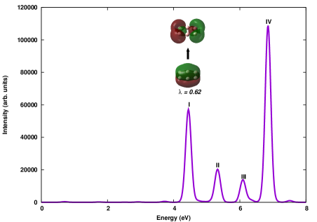
Figure 4.16: The linear optical absorption spectrum of planar ring B${}_{6}^{+}$ isomer (I), calculated using the CIS approach, along with the natural transition orbitals involved in the excited states corresponding to the peak I (4.44 eV). Parameter $\lambda$ refers to a fraction of the NTO pair contribution to a given electronic excitation.

Bulged wheel structure is the next low lying isomer of B${}_{6}^{+}$ with just 0.023 eV above the global minimum. However, as compared to the neutral one, this geometry has C₁ symmetry due to the significant bond length reordering. Our computed geometries are consistent with the results of Refs. ¹⁴², ¹⁴⁴. The optical absorption spectrum is presented in Fig. 4.17. The many-particle wavefunctions of excited states contributing to various peaks are presented in Table LABEL:Tab:table-cationic-bulged-wheel. The spectrum is distinctly different with a large number of smaller peaks and a stronger peak at 6.24 eV. The onset of spectrum occurs at 1.76 eV dominated by $H_{\beta}\rightarrow L_{\beta}$ and $H_{\beta}-1\rightarrow L_{\beta}$ configurations.

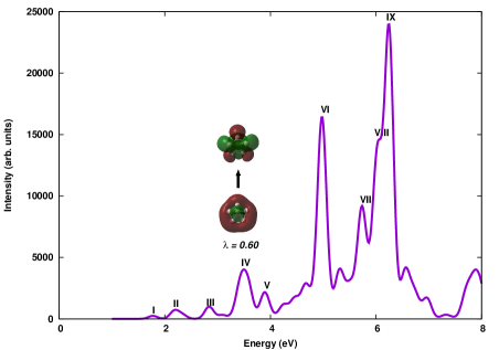
Figure 4.17: The linear optical absorption spectrum of bulged wheel B${}_{6}^{+}$ isomer, calculated using the CIS approach, along with the natural transition orbitals involved in the excited states corresponding to the peak IV (3.58 eV). Parameter $\lambda$ refers to a fraction of the NTO pair contribution to a given electronic excitation.

Another ring-like structure with D_2h symmetry and doublet multiplicity lies next in the energy order. The hexagonal benzene type structure has 1.66 Å and 1.53 Å as unique bond lengths, which are somewhat larger than those reported in the literature ^{142, 144}. The optical absorption spectrum presented in Fig. 4.18, is fairly simple and has well resolved peaks. The many-particle wavefunctions of excited states contributing to various peaks are presented in Table LABEL:Tab:table-cationic-planar-d2h-ring. All absorption peaks are due to the polarization along the plane of the isomer. The strongest absorption is seen at 3.52 eV with fully delocalized to partially localized nature of transition.

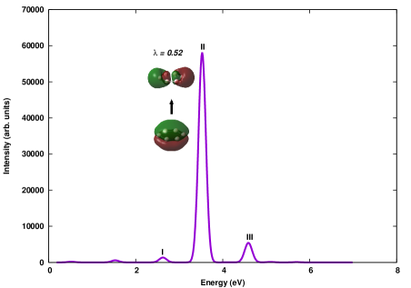
Figure 4.18: The linear optical absorption spectrum of planar ring B${}_{6}^{+}$ isomer II, calculated using the CIS approach, along with the natural transition orbitals involved in the excited states corresponding to the peak II (3.52 eV). Parameter $\lambda$ refers to a fraction of the NTO pair contribution to a given electronic excitation.

Next low lying isomer is a planar incomplete wheel structure with C_2v point group symmetry and quartet multiplicity. This multiplicity and computed geometry is consistent with results of Ref. ¹⁴⁴. The optical absorption (cf. Fig. 4.19) starts at 1.69 eV, with polarization transverse to the plane of the isomer. The many particle wave-functions of excited states contributing to various peaks are presented in Table LABEL:Tab:table-cationic-incomplete-wheel. The configurations contributing to the first peak are $H_{\beta}-2\rightarrow L_{\beta}$.

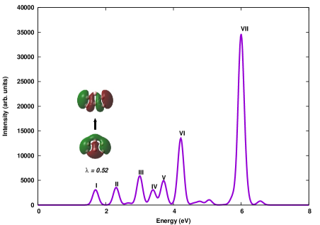
Figure 4.19: The linear optical absorption spectrum of incomplete wheel B${}_{6}^{+}$ isomer, calculated using the CIS approach, along with the natural transition orbitals involved in the excited states corresponding to the peak I (1.69 eV). Parameter $\lambda$ refers to a fraction of the NTO pair contribution to a given electronic excitation.

Another isomer with the same point group symmetry and multiplicity as that of the previous one, but having a geometry of linear chain with an isosceles triangle at the end, is the next low lying isomer of cationic B${}_{6}^{+}$. Our results about geometry are in good agreement with the Ref. ¹⁴⁴. The optical absorption spectrum (cf. Fig. 4.20) has three major peaks, coupled with a number of minor peaks. The first major peak occurs at 3.90 eV, with polarization along the plane of the isomer, and has dominant contribution from $H_{3\alpha}\rightarrow L_{\alpha}+1$ (cf. Table LABEL:Tab:table-cationic-threaded-trimer).

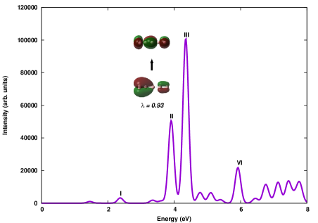
Figure 4.20: The linear optical absorption spectrum of threaded trimer B${}_{6}^{+}$ isomer, calculated using the CIS approach, along with the natural transition orbitals involved in the excited states corresponding to the peak II (3.90 eV). Parameter $\lambda$ refers to a fraction of the NTO pair contribution to a given electronic excitation.

Tetragonal bipyramid forms the next stable isomer of cationic B${}_{6}^{+}$, with D_4h point group symmetry and doublet multiplicity. This is in good agreement with the geometries reported in Refs. ¹⁴² and ¹⁴⁴. The optical absorption spectrum (cf. Fig. 4.21) has well defined small number of peaks. $H_{1\alpha}\rightarrow L_{\alpha}$ and $H_{\alpha}-4\rightarrow L_{\alpha}$ contributes dominantly to peaks in the visible range at 1.23 eV and 2.55 eV, respectively (cf. Table LABEL:Tab:table-cationic-triangular-bipyramid).

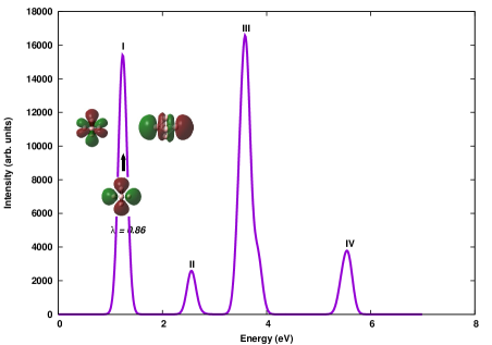
Figure 4.21: The linear optical absorption spectrum of triangular bipyramid B${}_{6}^{+}$ isomer , calculated using the CIS approach, along with the natural transition orbitals involved in the excited states corresponding to the peak I (1.23 eV). Parameter $\lambda$ refers to a fraction of the NTO pair contribution to a given electronic excitation.

Two more structures were found stable i.e. (a) a planar structure with two trimers joined together and, (b) a linear one. These isomers are much above the global minimum energy, it rules out their room temperature existence. In the linear isomer the absorption spectrum (cf. Fig. 4.22) is red-shifted as compared to the neutral one, with major peak at 4.25 eV with dominant contribution from $H_{\beta}-1\rightarrow L_{\beta}+1$ and $H_{\beta}\rightarrow L_{\beta}$ configurations. In case of planar trimers structure, the spectrum (cf. Fig. 4.23) also seems to be red shifted as compared to the neutral one. The first peak is found at 1.40 eV with $H_{\beta}\rightarrow L_{\beta}$ and $H_{\beta}-2\rightarrow L_{\beta}+1$, characterized by $\pi\rightarrow\pi^{*}$ transition, as dominant contribution to the wavefunction of the excited state.

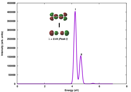
Figure 4.22: The linear optical absorption spectrum of linear B${}_{6}^{+}$ isomer , calculated using the CIS approach, along with the natural transition orbitals involved in the excited states corresponding to the peak I (4.25 eV). Parameter $\lambda$ refers to a fraction of the NTO pair contribution to a given electronic excitation.

Figure 4.23: The linear optical absorption spectrum of planar trimers B${}_{6}^{+}$ isomer , calculated using the CIS approach, along with the natural transition orbitals involved in the excited states corresponding to the peak I (1.40 eV). Parameter $\lambda$ refers to a fraction of the NTO pair contribution to a given electronic excitation.

4.3 Summary

A large number of randomly selected initial structures of neutral B₆ and cationic B${}_{6}^{+}$ clusters are taken into consideration for locating the global and local minimas on the potential energy curves. A careful geometry optimization is done for all those structures at a correlated level. The optical absorption spectra of different low-lying isomers of both neutral and cationic isomers are reported here. A singles configuration interaction approach was used to compute excited state energies and the absorption spectra of various clusters. Spectra of cationic clusters appear slightly red-shifted with respect to the neutral one. A comparison of spectra with CIS as well as more sophisticated EOM-CCSD method is presented in light of nature of excitations involved in the spectra. In all closed shell systems, a complete agreement on the nature of configurations involved is observed in both methods. On the other hand, for open-shell systems, minor contribution from double excitations are observed. Also, the spectra computed using EOM-CCSD approach is generally red-shifted as compared to the CIS ones. Such comparisons can be used to benchmark the CIS results.

Different isomers exhibit distinct optical response, even though they are isoelectronic and many of them are almost degenerate. This signals a strong-structure property relationship, which can be exploited for experimental identification of these isomers; something which is not possible with the conventional mass spectrometry. A strong mixture of configurations in the many-body wavefunctions of various excited states are observed, indicating the plasmonic nature of the photoexcited states ¹²⁶.

Chapter 5 Theory of Linear Optical Absorption in Various Isomers of Aluminum Clusters Al_n ($n$=2 – 5)

This chapter is based on a submitted manuscript, available on arxiv.org:1303.2511
by Ravindra Shinde and Alok Shukla.

Metal clusters are promising candidates in the era of nanotechnology. The reason behind growing interest in clusters lies in their interesting properties, applicability of simple theoretical models to describe their properties, and a vast variety of potential technological applications ^{1, 2, 3, 6, 16}.

Various jellium models have successfully described electronic structures of alkali metal clusters, because alkali metals have free valence electrons ⁶. This beautifully explains the higher abundance of certain clusters. However, in case of aluminum clusters, the experimental results often provide conflicting evidence about the size at which the jellium model would work ^{57, 145}. The theoretical explanation also depends on the valency of aluminum atoms considered. Since s - p orbital energy separation in aluminum atom is 4.99 eV, and it decreases with the cluster size, the valency should be changed from one to three ¹⁷. Perturbed jellium model, which takes orbital anisotropy into account, has successfully explained the mass abundance of aluminum clusters ^{146, 147}.

Shell structure and s - p hybridization in anionic aluminum clusters were probed using photoelectron spectroscopy by Ganteför and Eberhardt ¹⁴⁸, and Li et al. ⁵⁷. Evolution of electronic structure and other properties of aluminum clusters has been studied in many reports ^{17, 57, 146, 149, 150, 151, 152, 153, 154, 155, 156, 157, 158}. Structural properties of aluminum clusters were studied using density functional theory by Rao and Jena ¹⁷. An all electron and model core potential study of various Al clusters was carried out by Martinez et al. ¹⁵⁷. Upton performed chemisorption calculations on aluminum clusters and reported that Al₆ is the smallest cluster that will absorb H₂. DFT alongwith molecular dynamics were used to study electronic and structural properties of aluminum clusters ¹⁵⁴.

Although the photoabsorption in alkali metal clusters has been studied by many authors at various levels of theory ^{77, 78, 79, 81, 159, 160, 161, 162}, very few similar studies exist for aluminum clusters ^{163, 164}. Optical absorption in several aluminum clusters corresponding to the minimum energy configurations has been studied by Deshpande et al. using TDDFT ¹⁶³. Xie et al. presented TDDFT optical absorption spectra of various caged icosahedral aluminum clusters ¹⁶⁴. However, no theoretical or experimental study has been done on optical absorption in various low lying isomers of aluminum clusters. The distinction of different isomers of a cluster has to be made using an experimental or theoretical technique in which the properties are size, as well as shape, dependent. Conventional mass spectrometry only distinguishes clusters according to the masses. Hence, our theoretical results can be coupled with the experimental measurements of optical absorption, to distinguish between different isomers of a cluster. We have recently reported results of such calculation on small boron clusters ¹⁶⁵.

In this chapter, we present results of systematic calculations of optical absorption in various low lying isomers of small aluminum clusters using ab initio large-scale MRSDCI method. The nature of optical excitations involved in absorption has also been investigated by analyzing the wavefunctions of the excited states.

Remainder of the chapter is organized as follows. Next section discusses theoretical and computational details of the calculations, followed by section 5.2, in which results are presented and discussed. Conclusions and future directions are presented in section 5.3. A detailed information about wavefunctions of excited states contributing to various photoabsorption peaks is presented in the Appendix D.

5.1 Theoretical and Computational Details

The geometry of various isomers were optimized using the size-consistent coupled-cluster singles-doubles (CCSD) method, as implemented in the gaussian09 package ¹³⁸. A basis set of 6-311++G(2d,2p) was used which was included in the gaussian 09 package itself. This basis set is optimized for the ground state calculations. Since an even numbered electron system can have singlet, triplet, or higher spin multiplicity, we repeated the optimization for singlet and triplet systems to look for the true ground state geometry. Similarly, for odd numbered electron systems, doublet and quartet multiplicities were considered in the geometry optimization. To initiate the optimization, raw geometries, reported by Rao and Jena, based on density functional method were used ¹⁷. Figure 5.1 shows the final optimized geometries of the isomers studied in this chapter.

The linear photoabsorption spectra of various isomers of the boron clusters were computed using MRSDCI method, as described in subsection 2.1.2.3.

Our group has extensively used such approach in performing large-scale correlated calculations of linear optical absorption spectra of conjugated polymers ^{87, 88, 89, 90}, and atomic clusters ^{165, 166}. We have also frozen the chemical core of aluminum atom from virtual excitations and have put a cap on total number of virtual orbitals taking part in optical absorption based on the energy of the orbital, as done previously with boron clusters.¹⁶⁵

(a) Al₂, D_∞h, ${}^{\mathbf{3}}\mathbf{\bm{\Pi_{u}}}$

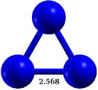
(b) Al₃, D_3h, $\bm{{}^{2}A_{1}^{{}^{\prime}}}$

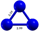
(c) Al₃, C_2v, $\bm{{}^{4}A_{2}}$

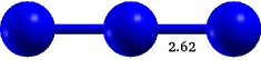
(d) Al₃, D_∞h, $\bm{{}^{4}\Sigma_{u}}$

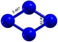
(e) Al₄, D_2h, $\bm{{}^{3}B{}_{2g}}$

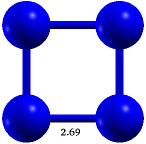
(f) Al₄, D_4h, $\bm{{}^{3}B{}_{3u}}$

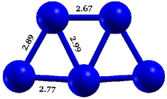
(g) Al₅, C_2v, $\bm{{}^{2}A{}_{1}}$

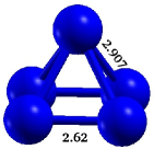
(h) Al₅, C_4v, $\bm{{}^{2}A{}_{1}}$

Figure 5.1: Geometry optimized structures of aluminum clusters with point group symmetry and the electronic ground state at the CCSD level. All numbers are in Å unit.

5.2 Results and Discussion

In this section, first we present a systematic study of the convergence of our results and various approximations used. In the latter part, we discuss the results of our calculations on various clusters.

5.2.1 Convergence of calculations

In this section we discuss the convergence of photoabsorption calculations with respect to the choice of the basis set, and the size of the active orbital space.

5.2.1.1 Choice of basis set

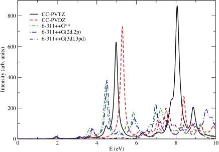
Figure 5.2: Optical absorption in Al₂ calculated using various Gaussian contracted basis sets.

In the literature several optimized basis sets are available for specific purposes, such as ground state optimization, excited state calculations etc. In an earlier work (see chapter 3), we have reported a systematic basis set dependence of photoabsorption of boron cluster ¹⁶⁵. Similarly, here we have checked the dependence of photoabsorption spectrum of aluminum dimer on basis sets used ^{123, 124} as shown in Fig. 5.2. The 6-311 type Gaussian contracted basis sets are known to be good for ground state calculations. The correlation consistent (CC) basis sets, namely, CC-polarized valence double-zeta and CC-polarized valence triple zeta (cc-pVTZ) give a good description of excited states of various systems. The latter is found to be more sophisticated in describing the high energy excitations, which were also confirmed using results of an independent TDDFT calculation ¹⁶⁷. Therefore, in this work, we have used the cc-pVTZ basis set for the optical absorption calculations.

5.2.1.2 Orbital truncation scheme

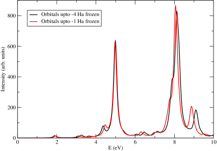
Figure 5.3: The effect of freezing the core orbitals of aluminum atoms on optical absorption spectrum of Al₂. It renders little effect on optical absorption spectrum, with significant reduction in the computational cost.

With respect to the total number of orbitals N in the system, the computational time in configuration interaction calculations scales as $\thickapprox$ N⁶. Therefore, such calculations become intractable for moderately sized systems, such as those considered here. So, in order to ease those calculations, the lowest lying molecular orbitals are constrained to be doubly occupied in all the configurations, implying that no optical excitation can occur from those orbitals. It reduces the size of the CI Hamiltonian matrix drastically. In fact, this approach is recommended in quantum chemical calculations, because the basis sets used are not optimized to incorporate the correlations in core electrons ⁸³. The effect of this approximation on the spectrum is as shown in Fig. 5.3. Since, calculations with all electrons in active orbitals were unfeasible, we have frozen occupied orbitals upto -4 Hartree of energy for the purpose of demonstration. The effect of freezing the core is negligibly small in the low energy regime, but shows disagreement in the higher energy range. However, for very high energy excitations, photodissociation may occur, hence absorption spectra at those energies will cease to have meaning. Thus, the advantage of freezing the core subdues this issue. Therefore, in all the calculations, we have frozen the chemical core from optical excitations.

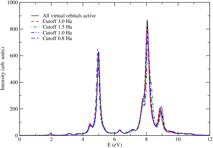
Figure 5.4: The effect of the number of active orbitals (N_act) on the optical absorption spectrum of Al₂. Until N_act=46, the optical spectrum does not exhibit any significant change. It corresponds to 1.0 Hartree ($\approx 27.2$ eV) virtual orbital energy.

Not only occupied, but high energy virtual (unoccupied) orbitals can also be removed from the calculations to make them tractable. In this case the high lying orbitals are constrained to be unoccupied in all the configurations. This move is justifiable, because it is unlikely that electrons would prefer partial filling of high energy orbitals in an attempt to avoid other electrons. However, this will only be applicable if the orbitals are sufficiently high in energy. Fig. 5.4 shows the effect of removing orbitals having more than the specified energy. From the figure it is clear that photoabsorption spectra exhibits no difference at all upto 1 Hartree cutoff on virtual orbitals. Below 0.8 Ha cutoff, the spectra start deviating from each other. Hence, we have ignored the virtual orbitals having energy more than 1 Ha.

5.2.1.3 Size of the CI expansion

[b]

Table 5.1: The average number of reference configurations (N_ref), and average number of total configurations (N_total) involved in MRSDCI calculations, ground state (GS) energies (in Hartree) at the MRSDCI level, relative energies and correlation energies (in eV) of various isomers of aluminum clusters.

Cluster	Isomer	Nref	Ntotal	GS energy	Relative	Correlation energy2
				(Ha)	energy (eV)	per atom(eV)
Al2	Linear	40	445716	-483.9063281	0.00	1.69
Al3	Equilateral triangular	40	1917948	-725.9053663	0.00	2.38
	Isosceles triangular	22	1786700	-725.8748996	0.83	2.36
	Linear	18	1627016	-725.8370397	1.85	2.16
Al4	Rhombus	13	3460368	-967.8665897	0.00	1.82
	Square	21	1940116	-967.8258673	1.11	1.80
Al5	Pentagonal	7	3569914	-1209.8114803	0.00	1.73
	Pyramidal	8	3825182	-1209.7836568	0.76	1.77

• The difference in Hartree-Fock energy and MRSDCI correlated energy of the ground state.

In the multi-reference CI method, the size of the Hamiltonian matrix increases exponentially with the number of molecular orbitals in the system. Also, accurate correlated results can only be obtained if sufficient number of reference configurations are included in the calculations. In our calculations, we have included those configurations which are dominant in the wavefunctions of excited states for a given absorption peak. Also, for ground state calculations, we included configurations until the total energy converges within a pre-defined tolerance. Table 5.1 shows the average number of reference configurations and average number of total configurations involved in the CI calculations of various isomers. For a given isomer, the average is calculated across different irreducible representations needed in these symmetry adapted calculations of the ground and various excited states. For the simplest cluster, the total configurations are about half a million and for the biggest cluster considered here, it is around four million for each symmetry subspace of Al₅. The superiority of our calculations can also be judged from the correlation energy defined here (cf. Table 5.1), which is the difference in the total energy of a system at the MRSDCI level and the Hartree-Fock level. The correlation energy per atom seems to be quite high for all the clusters, making our calculations stand out among other electronic structure calculations, especially single reference DFT based calculations.

5.2.2 MRSDCI photoabsorption spectra of various clusters

In this section, we describe the photoabsorption spectra of various isomers of the aluminum clusters studied. Graphical presentation of molecular orbitals involved are also given in each subsection below.

5.2.2.1 Al₂

Aluminum dimer is the most widely studied cluster of aluminum. It has now been confirmed that the Al₂ (cf. Fig. 5.1LABEL:sub@subfig:subfig-al2) has ${}^{3}\Pi_{u}$ ground state. The bond length obtained using geometry optimization at CCSD level was 2.72 Å with D_∞h point group symmetry. This is in very good agreement with available data, such as Martinez et al. obtained 2.73 Å as dimer length using all electron calculations ¹⁵⁷, 2.71 Å ¹⁵⁵ and 2.75 Å ¹⁶⁸ as bond lengths using DFT and configuration interaction methods, and 2.86 Å obtained using DFT with generalized gradient approximation ¹⁷. The experimental bond length of aluminum dimer is 2.70 Å ¹⁶⁹. Another metastable state of the dimer exists with ${}^{3}\Sigma_{g}^{-}$ electronic state, and 2.48 Å in bond length.

(a)

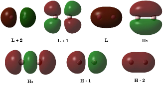
(b)

Figure 5.5: LABEL:sub@subfig:al2-lin-plot The linear optical absorption spectrum of Al₂, calculated using the MRSDCI approach. The peaks corresponding to the light polarized along the molecular axis are labeled with the subscript $\parallel$, while those polarized perpendicular to it are denoted by the subscript $\perp$. For plotting the spectrum, a uniform linewidth of 0.1 eV was used. LABEL:sub@subfig:al2-lin-mo Molecular orbitals of aluminum dimer. $H$ and $L$ stands for HOMO and LUMO respectively, and $H_{1}$ and $H_{2}$ are singly occupied degenerate molecular orbitals.

The many-particle wavefunction of Al₂ consists of two degenerate singly occupied molecular orbitals (to be denoted by $H_{1}$ and $H_{2}$, henceforth), because it is a spin triplet system. Similarly, the configurations involving excitations from occupied molecular orbitals to the unoccupied orbitals, form excited state wavefunctions. The computed photoabsorption spectrum of Al₂, as shown in Fig. 5.5LABEL:sub@subfig:al2-lin-plot, is characterized by weaker absorption at lower energies and couple of intense peaks at higher energies. The many-particle wavefunctions of excited states contributing to the peaks are presented in Table LABEL:Tab:table_al2_lin.

The spectrum starts with a small absorption peak at around 2 eV, characterized by $H_{2}\rightarrow L+1$ and light polarized along the direction of axis of the dimer. It is followed by a couple of small intensity peaks, until a dominant absorption is seen at 5 eV. This is characterized by $H_{1}\rightarrow L+3$. Another dominant peak is observed at 8 eV having $H-2\rightarrow L$ as dominant configuration, with absorption due to light polarized perpendicular to the axis of the dimer.

Our spectrum differs from the one obtained with the time-dependent local density approximation (TDLDA) method ¹⁶³ in both the intensity and the number of peaks. However, we agree with TDLDA¹⁶³ in predicting two major peaks at 5 eV and 8 eV. Unlike our calculations, the number of peaks is much more in TDLDA results and the spectrum is almost continuous. Minor peaks at 3.2 eV and 6.3 eV are also observed in the TDLDA spectrum of dimer. The latter one is, contrary to TDLDA spectrum, found to be a small peak in our calculations.

5.2.2.2 Al₃

Among the possible isomers of aluminum cluster Al₃, the equilateral triangular isomer is found to be the most stable. We have considered three isomers of Al₃, namely, equilateral triangle, isosceles triangle, and a linear chain. The most stable isomer has $D{}_{3h}$ point group symmetry, and ${}^{2}A_{1}^{{}^{\prime}}$ electronic state. The optimized bond length 2.57 Å, is in good agreement with reported theoretical values 2.61 Å ¹⁷, 2.62 Å ¹⁴⁶, 2.56 Å ¹⁵⁷, and 2.52 Å ^{150, 151}. The doublet ground state is also confirmed with the results of magnetic deflection experiments ¹⁵³.

The next isomer, which lies 0.83 eV higher in energy, is the isosceles triangular isomer. The optimized geometry has 2.59 Å, 2.59 Å and 2.99 Å as sides of triangle, with a quartet ground state (${}^{4}A_{2}$). Our results are in agreement with other theoretical results ^{146, 157, 154}.

Linear Al₃ isomer again with quartet multiplicity is the next low-lying isomer. The optimized bond length is 2.62 Å. This is in good agreement with few available reports ^{157, 154, 150}.

The photoabsorption spectra of these isomers are presented in Figs. 5.6LABEL:sub@subfig:plot-al3-equil, 5.7LABEL:sub@subfig:plot-al3-iso and 5.8LABEL:sub@subfig:plot-al3-lin. The corresponding many-body wavefunctions of excited states corresponding to various peaks are presented in Table LABEL:Tab:table_al3_equil_tri, LABEL:Tab:table_al3_iso_tri and LABEL:Tab:table_al3_lin_tri respectively. In the equilateral triangular isomer, most of the intensity is concentrated at higher energies. The same is true for the isosceles triangular isomer. However, the spectrum of isosceles triangular isomer appears slightly red shifted with respect to the equilateral counterpart. Along with this shift, there appears a split pair of peaks at 5.8 eV. This splitting of oscillator strengths might be due to distortion accompanied by symmetry breaking. The absorption spectrum of linear isomer is altogether different with bulk of the oscillator strength carried by peaks in the range 4 – 5 eV, and, due to the polarization of light absorbed parallel to the axis of the trimer.

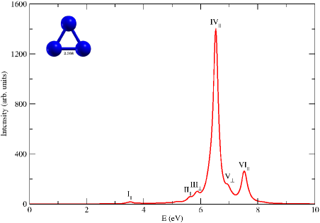
(a)

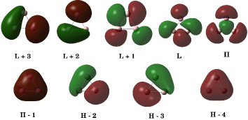
(b)

Figure 5.6: LABEL:sub@subfig:plot-al3-equil The linear optical absorption spectrum of Al₃ equilateral triangle isomer, calculated using the MRSDCI approach. The peaks corresponding to the light polarized along the molecular plane are labeled with the subscript $\parallel$, while those polarized perpendicular to it are denoted by the subscript $\perp$. For plotting the spectrum, a uniform linewidth of 0.1 eV was used. LABEL:sub@subfig:al3-equil-mo Molecular orbitals of equilateral triangular aluminum trimer. $H$ and $L$ stands for HOMO and LUMO respectively. ($H-2$, $H-3$), ($L$, $L+1$) and ($L+2$, $L+3$) are degenerate pairs.

The optical absorption spectrum of equilateral triangular isomer consists of very feeble low energy peaks at 3.5 eV, 5.6 eV and 5.8 eV characterized by $H-3\rightarrow L+5$, a double excitation $H-2\rightarrow L+5;H-1\rightarrow L+5$, and $H-3\rightarrow L+2$ respectively. The latter peak is due to the light polarized perpendicular to the plane of the isomer. It is followed by an intense peak at around 6.5 eV with dominant contribution from $H\rightarrow L+6$ and $H\rightarrow L+4$ configurations. A semi-major peak is observed at 7.5 eV characterized mainly due to double excitations.

Two major peaks at 6.5 eV and 7.5 eV in the spectrum of Al₃ equilateral isomer, obtained in our calculations are also found in the spectrum of TDLDA calculations, with the difference that the latter does not have a smaller intensity in TDLDA ¹⁶³. Other major peaks obtained by Deshpande et al. ¹⁶³ in the spectrum of aluminum trimer are not observed, or have very small intensity in our results.

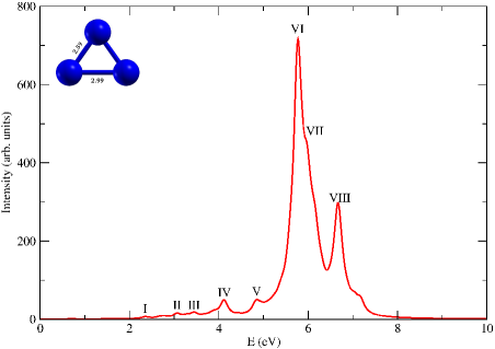
(a)

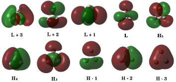
(b)

Figure 5.7: LABEL:sub@subfig:plot-al3-iso The linear optical absorption spectrum of Al₃ isosceles triangle isomer, calculated using the MRSDCI approach. All peaks labeled above correspond to the light polarized along the molecular plane. For plotting the spectrum, a uniform linewidth of 0.1 eV was used. LABEL:sub@subfig:mo-al3-iso Molecular orbitals of isosceles triangular aluminum trimer. $H$ and $L$ stands for HOMO and LUMO respectively, and $H_{1}$, $H_{2}$, and $H_{3}$ are singly occupied molecular orbitals.

As compared to the equilateral triangle spectra, the isosceles triangular isomer exhibit several small intensity peaks (cf. Fig. 5.7) in the low energy regime. The majority of contribution to peaks of this spectrum comes from in-plane polarized transitions, with negligible contribution from transverse polarized light. The spectrum starts with a feeble peak at 2.4 eV with contribution from doubly-excited configuration $H\rightarrow L+1;H-2\rightarrow L+2$. One of the dominant contribution to the oscillator strength comes from two closely-lying peaks at 5.8 eV. The wavefunctions of excited states corresponding to this peak show a strong mixing of doubly-excited configurations, such as $H-3\rightarrow L+1;H-2\rightarrow L$ and $H-2\rightarrow L+1;H-4\rightarrow L$. The peak at 6.7 eV shows absorption mainly due to $H\rightarrow L+10$.

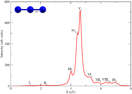
(a)

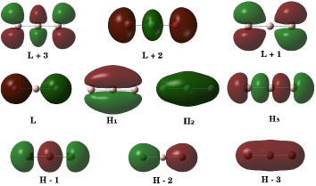
(b)

Figure 5.8: LABEL:sub@subfig:plot-al3-lin The linear optical absorption spectrum of Al₃ linear isomer, calculated using the MRSDCI approach. The peaks corresponding to the light polarized along the molecular axis are labeled with the subscript $\parallel$, while those polarized perpendicular to it are denoted by the subscript $\perp$. For plotting the spectrum, a uniform linewidth of 0.1 eV was used. LABEL:sub@subfig:mo-al3-lin Molecular orbitals of linear aluminum trimer. $H$ and $L$ stands for HOMO and LUMO respectively, and $H_{1}$, $H_{2}$, and $H_{3}$ are singly occupied molecular orbitals.

Linear trimer of aluminum cluster also shows low activity in the low energy range. Very feeble peaks are observed at 1.2 eV and 2.3 eV, both characterized by $H-3\rightarrow H-2$. This configuration also contributes to the semi-major peak at 4 eV along with $H-4\rightarrow H$. Two closely lying peaks at 4.3 eV and 4.6 eV carry the bulk of the oscillator strength. Major contribution to the former comes from $H-1\rightarrow L+2$ along with $H-3\rightarrow H-2$ being dominant in both the peaks. Again, as expected, the absorption due to light polarized along the trimer contributes substantially to the spectrum.

It is obvious from the spectra presented above that the location of the most intense absorption is quite sensitive to the structure, and thus can be used to distinguish between the three isomers.

5.2.2.3 Al₄

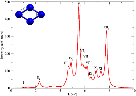
(a)

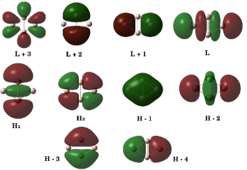
(b)

Figure 5.9: LABEL:sub@subfig:plot-al4-rho The linear optical absorption spectrum of rhombus Al₄, calculated using the MRSDCI approach. The peaks corresponding to the light polarized along the molecular axis are labeled with the subscript $\parallel$, while those polarized perpendicular to it are denoted by the subscript $\perp$. For plotting the spectrum, a uniform linewidth of 0.1 eV was used.LABEL:sub@subfig:mo-al4-rho Molecular orbitals of rhombus-shaped aluminum tetramer. $H$ and $L$ stands for HOMO and LUMO respectively, and $H_{1}$ and $H_{2}$ are singly occupied molecular orbitals.

Tetramer of aluminum cluster has many low lying isomers due to its flat potential energy curves. Among them, rhombus structure is the most stable with ${}^{3}B_{2g}$ electronic ground state. Our optimized bond length for rhombus structure is 2.50 Å and $63.8^{\circ}$ as the acute angle. This is to be compared with corresponding reported values of 2.56 Å and $69.3^{\circ}$ reported by Martinez et al. ¹⁵⁷, 2.51 Å and $56.5^{\circ}$ computed by Jones ¹⁵⁵, 2.55 Å and $67.6^{\circ}$ obtained by Schultz et al ¹⁵¹. We note that bond lengths are in good agreement but bond angles appear to vary a bit.

The other isomer studied here is an almost square shaped tetramer with optimized bond length of 2.69 Å. The electronic ground state of this $D_{4h}$ symmetric cluster is ${}^{3}B{}_{3u}$. This optimized geometry is in accord with 2.69 Å reported by Martinez et al. ¹⁵⁷, however, it is somewhat bigger than 2.57 Å calculated by Yang et al. ¹⁵⁰ and 2.61 Å obtained by Jones ¹⁵⁴.

For planar clusters, like rhombus and square shaped Al₄, two types of optical absorptions are possible: (a) planar – those polarized in the plane of the cluster, and (b) transverse – the ones polarized perpendicular to that plane. The many-particle wavefunctions of excited states contributing to the peaks are presented in Table LABEL:Tab:table_al4_rho and LABEL:Tab:table_al4_sqr. The onset of optical absorption in rhombus isomer occurs at around 1 eV with transversely polarized absorption characterized by $H_{1}\rightarrow L+1$. It is followed by an in-plane polarized absorption peak at 2.3 eV with dominant contribution from $H-2\rightarrow H_{1}$. Several closely lying peaks are observed in a small energy range of 4.5 – 8 eV. Peaks split from each other are seen in this range confirming that after shell closure, in perturbed droplet model, Jahn Teller distortion causes symmetry breaking usually associated with split absorption peaks. The most intense peak is observed at 5.5 eV characterized by $H-3\rightarrow L+4$.

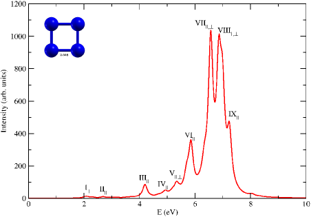
(a)

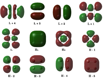
(b)

Figure 5.10: LABEL:sub@subfig:plot-al4-sqr The linear optical absorption spectrum of square Al₄, calculated using the MRSDCI approach. The peaks corresponding to the light polarized along the molecular plane are labeled with the subscript $\parallel$, while those polarized perpendicular to it are denoted by the subscript $\perp$. For plotting the spectrum, a uniform linewidth of 0.1 eV was used. LABEL:sub@subfig:mo-al4-sqr Molecular orbitals of square-shaped aluminum tetramer. $H$ and $L$ stands for HOMO and LUMO respectively, and $H_{1}$ and $H_{2}$ are singly occupied molecular orbitals.

The absorption spectrum of square shaped isomer begins with a couple of low in-plane polarized absorption peaks at 2.1 eV and 2.7 eV characterized by $H-1\rightarrow L$ and $H_{2}\rightarrow L+1$ respectively. The peak at 4.2 and 4.9 eV have $H-2\rightarrow L$ and $H_{1}\rightarrow L+2$ as respective dominant configurations. A major peak at 5.85 eV is observed with absorption due to in-plane polarization having $H-2\rightarrow L+2$ and a double excitation $H_{1}\rightarrow L+2;H-2\rightarrow L+2$ as dominant configurations. These configurations also make dominant contribution to the peak at 6.5 eV. This peak along with the one at 6.9 eV are two equally and most intense peaks of the spectrum. The latter has additional contribution from $H_{1}\rightarrow L+1;H-2\rightarrow L$. A shoulder peak is observed at 7.2 eV.

The TDLDA spectrum ¹⁶³ of aluminum rhombus tetramer differs from the one presented here. Peaks labeled III to XII in our calculated spectrum are also observed in the TDLDA results¹⁶³, however, the relative intensities tend to disagree. For example, the strongest absorption peak of TDLDA calculations is located around 7.9 eV, while in our spectrum we obtain the second most intense peak at that location. The highest absorption peak in our calculations is at 5.5 eV, while TDLDA does report a strong peak at the same energy¹⁶³, it is not the highest of the spectrum.

Our calculations also reveal a strong structure-property relationship as far as the location of the most intense peak in the absorption spectra of the two isomers is considered, a feature which can be utilized in their optical detection.

5.2.2.4 Al₅

The lowest lying pentagonal isomer of aluminum has $C_{2v}$ symmetry and has an electronic ground state of ${}^{2}A_{1}$. The bond lengths are as shown in Fig. 5.1LABEL:sub@subfig:geom-pentagon. These are slightly bigger than those obtained by Rao and Jena ¹⁷ and Yang et al. ¹⁵⁰ using the DFT approach. Many other reports have confirmed that the planar pentagon is the most stable isomer of $\textrm{Al}_{{}_{5}}$.

The other optimized structure of pentamer is perfect pyramid with $C_{4v}$ symmetry and ${}^{2}A_{1}$ electronic ground state. This lies 0.76 eV above the global minimum structure. This is the only three dimensional structure of Al cluster studied for optical absorption. The optimized geometry is consistent with those reported earlier by Jones ¹⁵⁴. However, it should be noted that there exists many more similar or slightly distorted structure lying equally close the the global minimum.

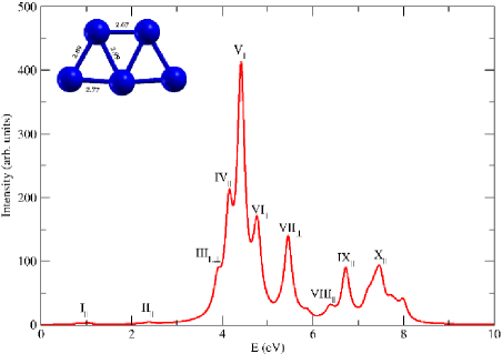
(a)

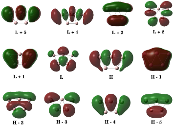
(b)

Figure 5.11: LABEL:sub@subfig:plot-al5-penta The linear optical absorption spectrum of pentagonal Al₅, calculated using the MRSDCI approach. The peaks corresponding to the light polarized along the molecular axis are labeled with the subscript $\parallel$, while those polarized perpendicular to it are denoted by the subscript $\perp$. For plotting the spectrum, a uniform linewidth of 0.1 eV was used. LABEL:sub@subfig:mo-al5-penta Molecular orbitals of pentagonal aluminum pentamer. $H$ and $L$ stands for HOMO and LUMO respectively.

The many-particle wavefunctions of excited states contributing to the peaks are presented in Table LABEL:Tab:table_al5_pentagon and LABEL:Tab:table_al5_pyramid. The optical absorption spectrum of pentagonal Al₅ has few low energy peaks followed by major absorption at 4.4 eV. It has dominant contribution from $H-1\rightarrow L+5$ configuration. Pentagonal isomer shows more optical absorption in the high energy range, with peaks within regular intervals of energy.

Few feeble peaks occur in the low energy range in the optical absorption of pyramidal isomer. The major absorption peak at 4.2 eV is slightly red-shifted as compared to the pentagonal counterpart. It is characterized by $H-3\rightarrow L+2$. A peak at 6 eV is seen in this absorption spectrum having dominant contribution from $H\rightarrow L+13$, which is missing in the spectrum of pentagon. These differences can lead to identification of isomers produced experimentally.

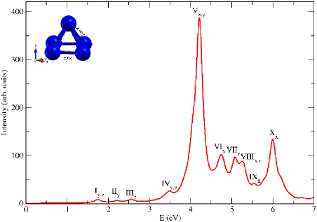
(a)

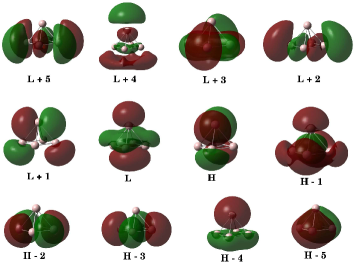
(b)

Figure 5.12: LABEL:sub@subfig:plot-al5-pyra The linear optical absorption spectrum of pyramidal Al₅, calculated using the MRSDCI approach. The peaks corresponding to the light polarized along the Cartesian axes are labeled accordingly. For plotting the spectrum, a uniform linewidth of 0.1 eV was used. LABEL:sub@subfig:plot-al5-pyra Molecular orbitals of pyramidal aluminum pentamer. $H$ and $L$ stands for HOMO and LUMO respectively.

In the range of spectrum studied in our calculations, the TDLDA calculated spectrum ¹⁶³ of pentagonal isomer is found to be similar to the one presented here as far as the peak locations are concerned, albeit the intensity profile differs at places. A small peak at 2.4 eV is observed in both the spectra, followed by peaks at 3.9 eV, 4.2 eV and 4.4 eV. These three peaks are also observed in TDLDA results with a little bit of broadening. Again, the peak at 5.4 eV matches with each other calculated from both the approaches. Peak found at 6.7 eV is also observed in the TDLDA calculation¹⁶³. Within the energy range studied here, the strongest peak position and intensity of this work is in good agreement with that of its TDLDA counterpart¹⁶³.

5.2.3 Nature of Optical Excitations

If an absorption peak is caused by an interaction among many particle-hole excitations (i.e. configurations) with comparable weights, it suggests a plasmon-like collective excitation as compared to molecular excitation dominated by a single configuration.¹²⁶ The wavefunctions of the excited states contributing to most of the peaks in the optical absorption spectra of clusters studied here exhibit strong configuration mixing, instead of being dominated by single configurations, pointing to the plasmonic nature of the optical excitations ¹²⁶.

In order to draw a distinction between two cases, we provide the results of calculations of Al₂H₂ cluster. The MRSDCI calculated optical absorption spectrum is as shown Fig. 5.13.

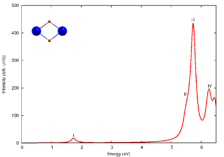
Figure 5.13: The linear optical absorption spectrum of Al₂H₂, calculated using the MRSDCI approach. For plotting the spectrum, a uniform linewidth of 0.1 eV was used.

Table 5.2: Excitation energies ($E$) and many-particle wavefunctions of excited states corresponding to the peaks in the linear absorption spectrum of Al₂H₂, along with the oscillator strength ($f_{12}$) of the transitions. In the wavefunction, the bracketed numbers are the CI coefficients of a given electronic configuration. Symbols $H$, and $L$, denote HOMO and LUMO orbitals respectively. $HF$ denotes the Hartree-Fock configuration.

Peak	$E$ (eV)	$f_{12}$	Wave Function
GS			$|HF\rangle$ (0.8961)
			$|H\rightarrow L+6\rangle$(0.1234)
I	1.73	0.1455	$|H\rightarrow L\rangle$(0.8874)
			$|H\rightarrow L+8\rangle$(0.1654)
II	5.57	0.3465	$|H\rightarrow L+3\rangle$(0.8000)
			$|H-1\rightarrow L+1\rangle$(0.2991)
III	5.74	3.5591	$|H\rightarrow L+4\rangle$(0.8041)
			$|H\rightarrow L;H\rightarrow L+2\rangle$(0.2745)
IV	6.23	0.5937	$|H-1\rightarrow L+2\rangle$(0.7316)
			$|H\rightarrow L+4;H\rightarrow L+2\rangle$(0.3112)

The many-particle wavefunctions of the excited states contributing to the peaks of Al₂H₂ (cf. Table 5.2) do not show a strong configuration mixing, rather, one single hole-particle excitation is seen to be dominant till 6.2 eV. Therefore, the nature of excitation in Al₂H₂ is of molecular type. Comparing the excited state wave functions of Al₂H₂ with those of the Al₂ cluster, we see a clear indication of strong configuration mixing in the latter, suggesting plasmonic nature of optical excitations. In other words, the closed-shell hydrogenated Al dimer has molecular type of optical excitations, while the open-shell bare Al dimer exhibits plasmonic type excitations.

5.3 Summary

In this study, we have presented large-scale all-electron correlated calculations of optical absorption spectra of several low-lying isomers of aluminum clusters Al_n, (n=2–5). Both ground and excited state calculations were performed at MRSDCI level, which take electron correlations into account at a sophisticated level. We have analyzed the nature of low-lying excited states. Isomers of a given cluster show a distinct signature spectrum, indicating a strong-structure property relationship. This fact can be used in experiments to distinguish between different isomers of a cluster. Owing to the sophistication of our calculations, our results can be used for benchmarking of the absorption spectra. The optical excitations involved are found to be collective type, and plasmonic in nature.

Our results were found to be significantly different as compared to the TDLDA results¹⁶³, for the clusters studied here. Given the fact that the MRSDCI calculations incorporate electron-correlation effect quite well both for the ground and the excited states, they could be treated as benchmarks, and be used to design superior TDDFT approaches.

Chapter 6 Linear Optical Absorption in Boron Wheel-Like Clusters B₇, B₈ and B₉: Benchmarking TDDFT against EOM-CCSD

Planar boron clusters, in particular, have proven to be interesting because of the multiple aromaticities and extreme coordination environments.^{11, 62, 63, 64, 128} Atoms of boron can adopt such an arrangement that they form a miniature wheel, with one atom at the center. B${}_{13}^{+}$ and B${}_{19}^{-}$ perform Wankel motor action when shined by circularly polarized light.^{72, 73, 127} Such clusters have been synthesized and their electronic structure is now well known.⁶⁴ Boron with seven, eight and nine atoms form such truly planar wheel structures with radii of 1.65 Å, 1.80 Å and 2.0 Å respectively. Although a lot of information about planarity, electronic structure and chemical bonding is now available, optical absorption of these clusters remains unexplored.

In order to describe the ground state of a system, normally, a reference state is used, which is a good approximation to the exact ground state of the system. Typically, one prefers variational approaches, although that is not the only possible way. This single reference state may not be the natural choice when it comes to the computation of excited states. Coupled cluster methods offer insensitivity to such single reference state for excited state calculations owing to the exponential treatment of single excitation effects.¹⁷⁰

Equation-of-motion coupled cluster (EOM-CC) is one of the approaches which can effectively and unambiguously describe excited states of molecules, polyradicals where ground or excited state is often degenerate. Since it does not make any assumptions about nature of the states, it is easy to use single reference method. It is most accurate in calculating one electron vertical transition states. Often, the cluster expansion is terminated at doubles, for computational feasibility without serious compromise on quality of results. The results can always be systematically improved by including more excitation levels. However, the method scales as N⁶, N being the number of basis functions, thereby making it intractable for large molecules.

We give here an account of other less expensive excited state calculation methods that can approximate the accurate EOM-CCSD results. In particular, the time-dependent density functional theory with adiabatic approximation continues to remain favorite for study of large variety of systems. The exact exchange and correlation functional required in this approach is not known, several approximations are made in that respect. This adds to the puzzle to choose the right functional for a given type of calculation. This work will provide qualitative as well as quantitative analysis of benchmarking results of single reference quantum chemical methods – TDDFT with different functionals against EOM-CCSD method. This study will help in identifying computationally the least expensive functional which mimic more accurate EOM-CCSD results of optical absorption.

The rest of the chapter is organized as follows. Next section discusses theoretical and computational details of the calculations, followed by section 6.2, in which results are presented and discussed. Conclusions and future directions are presented in section 6.3.

6.1 Theoretical and Computational Details

6.1.1 Geometry Optimization

The geometries of the boron wheel clusters, B₇, B₈ and B₉ were optimized using the computer code gaussian 09¹³⁸ employing a 6-311++G(2d,2p) basis set, and using the size-consistent CCSD method. To initiate the optimization, raw geometries, reported by Wang et al, based on density functional method were used.⁶⁴ The results of optimization are in accordance with the available report. ⁶⁴ These optimized geometries were further used in the calculations of optical absorption spectra. Figure 6.1 shows the final optimized geometries of the clusters studied in this paper.

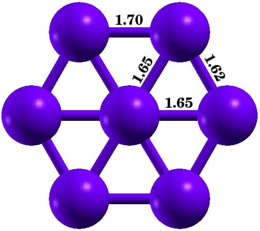
(a) B₇, D_2h, ${}^{2}B_{2g}$

(b) B₈, D_7h, ${}^{3}A_{g}$

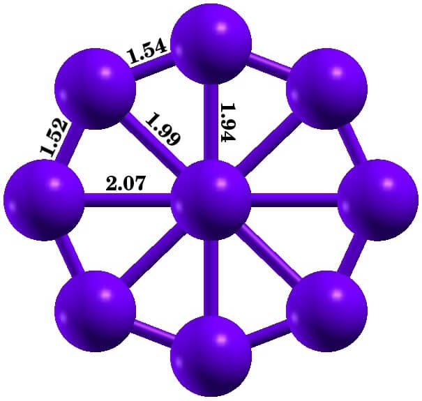
(c) B₉, D_2h, ${}^{2}B_{1g}$

Figure 6.1: Geometry optimized structures of boron wheels with point group symmetry and the electronic ground state. All numbers are in Angstrom unit.

The optical absorption spectra of these optimized geometries of the clusters are then calculated using EOM-CCSD and TDDFT. Various exchange and correlation functionals were used to compute the optical absorption spectra using TDDFT approach. An augmented correlation consistent polarized valence double zeta (aug-cc-pVDZ) basis set was used for all methods mentioned above.

6.1.2 Excited State Calculation Methods

Coupled cluster method is known to include electron correlation in a systematic manner. Coupled cluster is an exact formalism if all possible excitation are taken into account. Often, the excitation level is terminated at doubles, which gives rise to CCSD method. This method is extended to excited state calculations through what is known as Equation-of-Motion CCSD (EOM-CCSD).^{139, 92} The EOM-CC approach amounts to diagonalizing the effective Hamiltonian $e^{-T}He^{-T}$. The computational time for this approach scales as N⁶, where N is the number of basis functions, thereby limiting its use to smaller molecules.

Development of Density functional theory has led to enormous progress in the understanding of properties of various systems. However, the main drawback is, results depend upon the choice of energy functional used to perform the calculation. Many different functionals are proposed for various kinds of calculations and the number is still increasing. In the adiabatic approximation, the time-dependent counterpart of DFT, also uses the same functionals to investigate excited state properties. Here, we have considered various DFT functionals of various types to study the excited state properties and optical absorption in boron clusters. The set of functionals includes (a) Hybrid Generalized-Gradient Approximation (H-GGA) – PBE0¹⁷¹, B3LYP¹⁷², B3PW91¹⁷³ (b) Global Hybrid-Meta GGA (HM-GGA) – M06¹⁷⁴, M06-2X¹⁷⁴ (c) Long-range corrected – $\omega$B97xD¹⁷⁵, CAM-B3LYP¹⁷⁶, LC-$\omega$PBE¹⁷⁷.

6.2 Benchmarking: Photoabsorption Spectra of Wheel Clusters

In this section, we present the photoabsorption spectra of boron wheel clusters studied. Graphical presentation of natural transition orbitals involved in the case of TDDFT calculations are also given below. The many-particle wavefunctions of excited states contributing to the peaks of EOM-CCSD spectra are presented in Table LABEL:Tab:table-b7-eomccsd, LABEL:Tab:table-b8-eomccsd and LABEL:Tab:table-b9-eomccsd.

6.2.1 B₇

Figure 6.2: The linear optical absorption spectrum of boron wheel B₇ cluster, calculated using the EOM-CCSD approach.

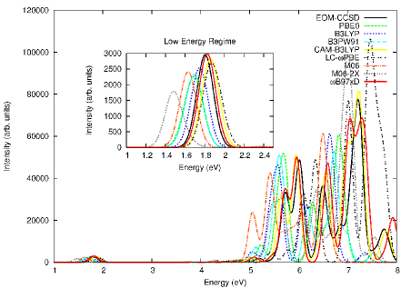
(a) Optical absorption spectrum of B₇ cluster

Figure 6.3: LABEL:sub@subfig:subfig-b7-eom-tddft-plot The linear optical absorption spectrum of boron wheel B₇ cluster, calculated using the TDDFT approach using various functionals, and compared to the spectrum calculated using EOM-CCSD. LABEL:sub@subfig:subfig-b7-nto-1-2 and LABEL:sub@subfig:subfig-b7-nto-3-4: Natural transition orbitals (NTO) involved in the excited states of B₇ cluster, calculated using PBE0 method corresponding to the peak at 1.63 eV with $\lambda$ = 0.56 ($H_{\alpha}-1\rightarrow L_{\alpha}$) and to the peak at 5.72 eV with $\lambda$ = 0.35 ($H_{1\alpha}\rightarrow L_{\alpha}+4$). Parameter $\lambda$ refers to a fraction of the NTO pair contribution to a given electronic excitation.

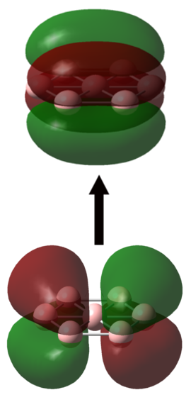
(b) $\lambda$ = 0.56 at 1.63eV

(c) $\lambda$ = 0.35 at 5.72eV

An excellent agreement is observed between EOM-CCSD and TDDFT results (cf. Fig. 6.3aLABEL:sub@subfig:subfig-b7-eom-tddft-plot) with $\omega$B97xD and CAM-B3LYP functionals. This agreement holds good both for excitation energies and oscillator strengths. However, $\omega$B97xD deviates from CAM-B3LYP spectra after 7 eV. M06 and M06-2X functionals show consistently red-shifted absorption throughout the spectrum. Other functionals, such as, PBE0 and B3PW91 almost overlap to each other in the low energy regime. However, former blue-shifts from B3PW91 at higher energies. NTO analysis of PBE0 spectrum (cf. Fig. 6.3aLABEL:sub@subfig:subfig-b7-nto-1-2, 6.3aLABEL:sub@subfig:subfig-b7-nto-3-4) reveals that the nature of excitation for the peak at 1.63 eV is $\pi\rightarrow\pi^{*}$, and at 5.72 eV, $\sigma\rightarrow\sigma^{*}$ dominates the excitation.

6.2.2 B₈

Figure 6.4: The linear optical absorption spectrum of boron wheel B₈ cluster, calculated using the EOM-CCSD approach.

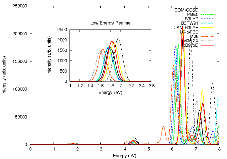
(a)

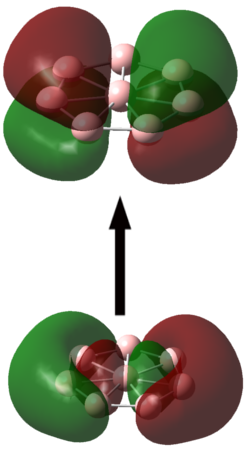
(b) $\lambda$ = 0.99 at 1.77eV

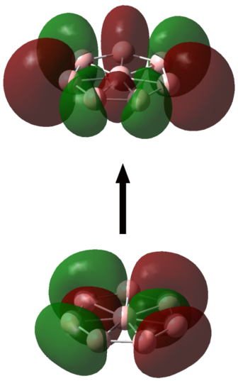
(c) $\lambda$ = 0.11 at 6.28eV

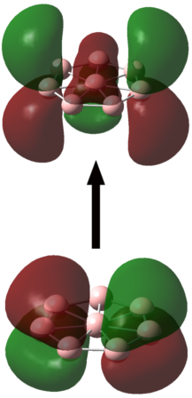
(d) $\lambda$ = 0.25 at 6.28eV

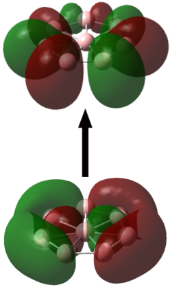
(e) $\lambda$ = 0.29 at 6.28eV

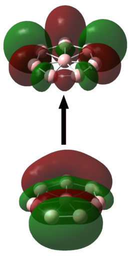
(f) $\lambda$ = 0.29 at 6.28eV

Figure 6.5: LABEL:sub@subfig:b8-eom-tddft-plot The linear optical absorption spectrum of boron wheel B₈ cluster, calculated using the TDDFT approach using various functionals, and compared to the spectrum calculated using EOM-CCSD. Natural transition orbitals involved in the excited states of B₈ cluster, calculated using PBE0 method corresponding to LABEL:sub@subfig:subfig-b8-nto-1-2 the peak at 1.77 eV with $\lambda$ = 0.99 ($H_{\beta}-1\rightarrow H_{1\beta}$ and $H_{\beta}-2\rightarrow H_{2\beta}$) and LABEL:sub@subfig:subfig-b8-nto-5-6 to the peak at 6.28 eV with $\lambda$ = 0.11 ($H_{\alpha}-2\rightarrow L_{\alpha}+3$), LABEL:sub@subfig:subfig-b8-nto-7-8 0.25 ($H_{\alpha}-1\rightarrow L_{\alpha}+2$) , LABEL:sub@subfig:subfig-b8-nto-9-10 0.29 ($H_{\beta}-2\rightarrow L_{\beta}+1$), LABEL:sub@subfig:subfig-b8-nto-11-12 0.29 ($H_{\beta}-1\rightarrow L_{\beta}$). Parameter $\lambda$ refers to a fraction of the NTO pair contribution to a given electronic excitation.

The optical absorption spectrum of B₈, Figs. 6.4 and 6.5, shows a small number of well-separated peaks. CAM-B3LYP and $\omega$B97xD gives an excellent agreement on absorption spectrum when compared to EOM-CCSD results. At the strongest absorption peak, both energies and intensity of spectrum of these functionals match very well with each other in this case. M06 provide poor performance in this case, with bands are shifted to lower energies. Also, there are extra peaks observed at higher energies for this functional. M06-2X seems to correct the latter behavior, while retaining the red-shift of bands. PBE0, B3LYP and B3PW91 spectra agree with each other at lower energies, but start deviating afterwards. The long-range corrected functional LC-$\omega$PBE has same intensity profile as that of EOM-CCSD, but the peaks are generally blue-shifted by 0.2–0.4 eV. A pair of $\sigma\rightarrow\pi^{*}$ transition takes place at 1.77 eV, as seen in the PBE0 NTO analysis in Fig. 6.5LABEL:sub@subfig:subfig-b8-nto-1-2.

6.2.3 B₉

Figure 6.6: The linear optical absorption spectrum of boron wheel B₉ cluster, calculated using the EOM-CCSD approach.

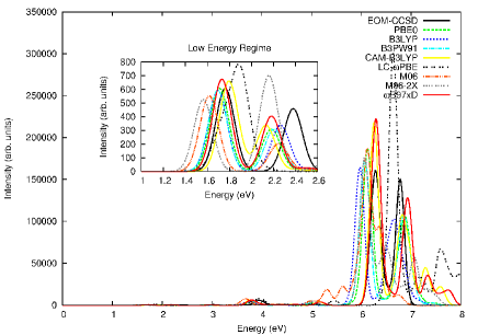
(a)

Figure 6.7: LABEL:sub@subfig:subfig-b9-eom-tddft-plot The linear optical absorption spectrum of boron wheel B₉ cluster, calculated using the TDDFT approach using various functionals, and compared to the spectrum calculated using EOM-CCSD approach. LABEL:sub@subfig:subfig-b9-nto-1-2 Natural transition orbitals (NTO) involved in the excited states of B₉ cluster, calculated using PBE0 method corresponding to the peak at 1.71 eV with $\lambda$ = 0.99 ($H_{\beta}-3\rightarrow H_{1\beta}$), and LABEL:sub@subfig:subfig-b9-nto-3-4 to the peak at 6.15 eV with $\lambda$ = 0.25 ($H_{\beta}-3\rightarrow L_{\beta}+1$) and LABEL:sub@subfig:subfig-b9-nto-5-6 $\lambda$ = 0.32 ($H_{\beta}-2\rightarrow L_{\beta}$). Parameter $\lambda$ refers to a fraction of the NTO pair contribution to a given electronic excitation.

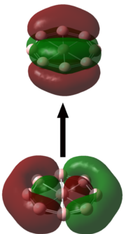
(b) $\lambda$ = 0.99 at 1.71eV

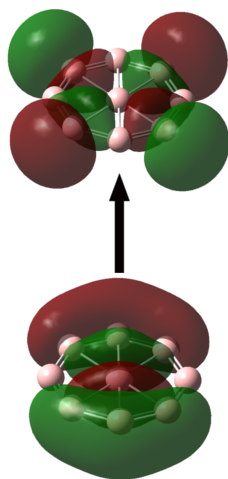
(c) $\lambda$ = 0.25 at 6.15eV

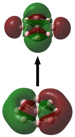
(d) $\lambda$ = 0.32 at 6.15eV

The optical absorption spectrum of B₉ also has a very few intense peaks. Almost negligible absorption is seen at lower energies. Compared to EOM-CCSD results, the functionals PBE0, B3LYP, B3PW91, M06 and M06-2X underestimate the peak position (cf. Fig. 6.7aLABEL:sub@subfig:subfig-b9-eom-tddft-plot). The spectrum of B₉ is extremely overestimated by LC-$\omega$PBE both in position and in the oscillator strengths. CAM-B3LYP and $\omega$B97xD again provides an excellent agreement with EOM-CCSD results on intensities as well as position of energy bands. Peak at 1.71 eV is dominated by $\sigma\rightarrow\pi^{*}$ and at 6.15 eV, $\sigma\rightarrow\sigma^{*}$ transitions take place, as evident from the NTO analysis shown in Fig. 6.7a.

6.3 Summary

The goal of the present study is to benchmark various exchange-correlation functionals used in TDDFT for calculating optical absorption spectra of planar boron wheel clusters. We compared results of TDDFT with eight different functionals to the results of a wavefunction based EOM-CCSD approach.

Hybrid GGA functionals – PBE0, B3LYP and B3PW91 – are poor performers as they tend to underestimate the excitations energies. Meta-GGA functionals M06 and M06-2X –which includes terms that depend on kinetic energy density – also underestimate the excitation energies. Among the long-range corrected functionals CAM-B3LYP provides the best agreement with EOM results on the basis of excitation energies as well as spectrum profile. This fact has also been confirmed in other benchmarking studies done previously.^{178, 179}

The contribution of configurations to the many-body wavefunctions of various excited states suggest that the excitations involved are of molecular type.^{126, 136} Since most of the absorption takes place at higher energies, these clusters could potentially be used as ultraviolet absorbers.

Although this study neither includes all the functionals available nor does the test cases are comprehensive, it helps in providing reasonable comparison between the current gold standard single reference method, namely, EOM-CCSD and TDDFT, by identifying the functionals which provide results as good as EOM-CCSD in light of optical absorption calculations. These findings can be tested against more sophisticated multi-reference calculations. Such high-level calculations are necessary to design superior yet less time-consuming TDDFT approaches.

Chapter 7 Theory of Linear Optical Absorption in Various Isomers of Magnesium Clusters Mg_n ($n$=2 – 5)

Clusters of group II elements, such as magnesium, are of special interest because they have two valence electrons, quasi-filled closed shells, and in bulk they are metals. In the case of small clusters, the bonding between atoms is expected to be of van der Walls type. This is evident in the case of extensively studied magnesium dimer. It exhibits large bond length of 3.92 Å and 0.034 eV/atom binding energy. However it is seen that, for larger clusters this bonding becomes stronger. Thus, study of divalent metals is appropriate for evolution of various cluster properties and to test various theoretical methods. Involvement of metal atoms in the clusters makes theoretical treatment a demanding task, mainly because of several nearly degenerate electronic states. In such situations, only multi-reference configuration interaction methods or coupled cluster singles doubles with perturbative triples (CCSD(T)) is known to provide best qualitative results. ¹⁸⁰ Since in this chapter, we are dealing with small sized clusters of magnesium, treated at a large-scale multi-reference configuration interaction singles doubles level of theory, the results will be superior to other ab initio quantum chemical methods.

There has been an enormous study of equilibrium geometry and electronic structure of small magnesium clusters. ^{180, 181, 182, akola_mg_epjd, 183, 184, 185, 186, 187} Andrey et al.¹⁸⁷ studied evolution of electronic structure of magnesium clusters with cluster size using all-electron density functional theoretical method. An evolution from non-metal to metal was explained using a gradient-corrected DFT calculations by Jellinek and Acioli¹⁸⁴ and by Akola et al. ¹⁸⁵ Larger clusters were studied at DFT level by Köhn et al.¹⁸⁰ Kumar and Car performed ab initio density functional molecular dynamics study of smaller magnesium clusters within local density approximation.¹⁸¹ Stevens and Krauss calculated electronic structure of ground and excited states of Mg dimer using multi-configurational self consistent field method. ¹⁸³ Kaplan, Roszak and Leszczynski investigated the nature of binding in the magnesium trimer at Møller - Plesset Perturbation Theory 4^th order (MP4) level.¹⁸⁶

The optical absorption in dimer was studied experimentally by McCaffrey and Ozin in Ar, Kr and Xe matrices ¹⁸² and by Balfour and Douglas. ¹⁸⁸ Solov’yov et al. calculated optical absorption spectra of global minimum structures of magnesium clusters using TDDFT and compared the spectra with results of classical Mie theory.¹⁸⁹ However, to best of our knowledge, no other experimental or theoretical study exists for optical absorption and excited states calculations of various low-lying isomers of magnesium clusters. The distinction of different isomers of a cluster has to be made using an experimental or theoretical technique in which the properties are size, as well as shape, dependent. Conventional mass spectrometry only distinguishes clusters according to the masses. We have addressed this issue by performing large-scale correlated calculations of optical absorption spectra of various isomers of magnesium clusters Mg_n (n=2–5), at MRSDCI level of theory. Hence, our theoretical results can be coupled with the experimental measurements of optical absorption, to distinguish between different isomers of a cluster. Using this approach, we have reported results of such calculation on small boron and aluminum clusters ^{165, 190}.

In this chapter, we present results of systematic calculations of optical absorption in various low-lying isomers of magnesium clusters using ab initio large-scale MRSDCI method. The nature of optical excitations involved in absorption has also been investigated by analyzing the wavefunctions of the excited states. Also, wherever possible, the results are compared with available literature.

Remainder of the chapter is organized as follows. Next section discusses theoretical and computational details of the calculations, followed by section 7.2, in which results are presented and discussed. Conclusions and future directions are presented in section 7.3. A detailed information about wavefunctions of excited states contributing to various photoabsorption peaks is presented in the Appendix Table LABEL:Tab:table_mg2_lin – LABEL:Tab:table_mg5_param.

7.1 Theoretical and Computational Details

The geometry of various isomers were optimized using the size-consistent coupled-cluster singles-doubles (CCSD) method, as implemented in the gaussian09 package ¹³⁸. A basis set of 6-311+G(d) was used which was included in the gaussian 09 package itself. This basis set is optimized for the ground state calculations. Different spin multiplicities of the isomers were taken into account for the optimization to determine the true ground state geometry. The process of optimization was initiated by using the geometries reported by Lyalin et al.¹⁸⁷, based upon first principles DFT based calculations. Figure 7.1 shows the final optimized geometries of the isomers studied in this chapter.

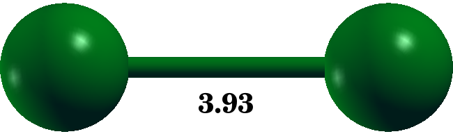
(a) Mg₂, D_∞h, ${}^{\mathbf{1}}\mathbf{\bm{\Sigma_{g}}}$

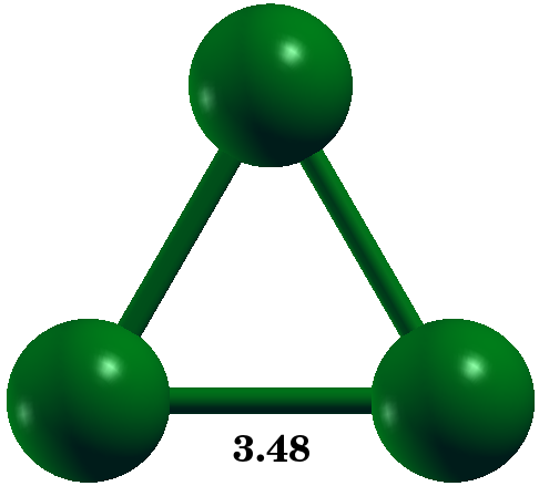
(b) Mg₃, D_3h, $\bm{{}^{1}A_{1}^{{}^{\prime}}}$

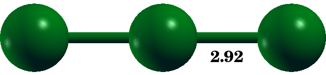
(c) Mg₃, D_∞h, $\bm{{}^{3}\Pi_{u}}$

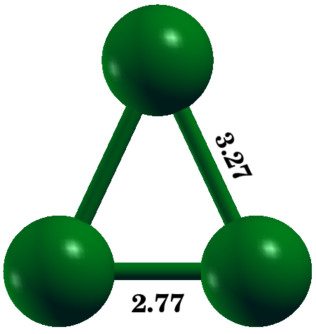
(d) Mg₃, C_2v, $\bm{{}^{3}A_{2}}$

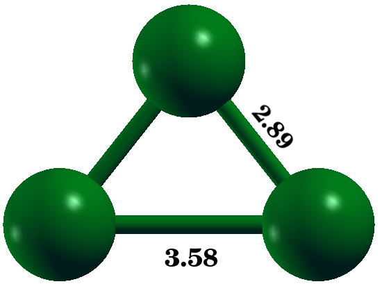
(e) Mg₃, C_2v, $\bm{{}^{3}B_{1}}$

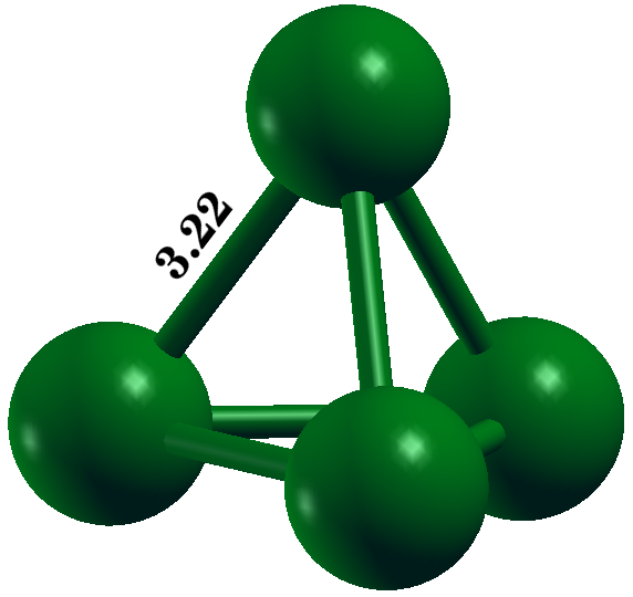
(f) Mg₄, T_d, $\bm{{}^{1}A{}_{1}}$

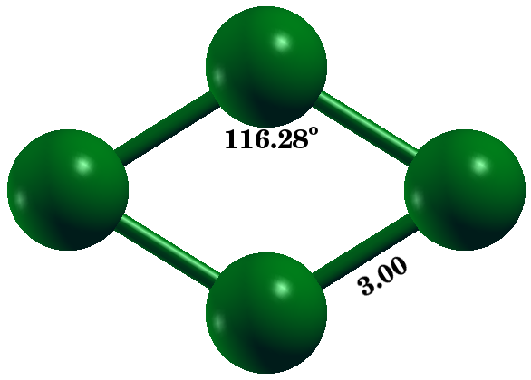
(g) Mg₄, D_2h, $\bm{{}^{3}B{}_{3u}}$

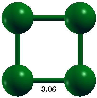
(h) Mg₄, D_4h, $\bm{{}^{3}B{}_{2u}}$

(i) Mg₅, D_3h, $\bm{{}^{1}A{}_{1}^{{}^{\prime}}}$

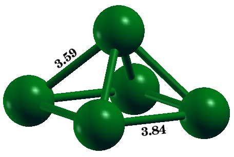
(j) Mg₅, C_4v, $\bm{{}^{1}A{}_{1}}$

Figure 7.1: Geometry optimized structures of magnesium clusters with point group symmetry and the electronic ground state at the CCSD level. All numbers are in Å unit.

If the total number of orbitals used in a CI expansion is $N$, the number of configurations in the calculation proliferates as $\approx N^{6}$, which can become intractable for large values of $N$. To reduce the computation, we employed the so-called “frozen-core approximation”, in which no virtual transitions are allowed from the chemical core orbitals of magnesium.

The linear photoabsorption spectrum of magnesium dimer was computed using full configuration interaction method. The spectra of various isomers of the remaining magnesium clusters were computed using MRSDCI method, as described in subsection 2.1.2.3.

7.1.1 Choice of Basis Set

Electronic structure calculations generally depend upon the size and the quality of basis set used. To explore the basis set dependence of computed spectra, we used several basis sets^{123, 124} to compute the optical absorption spectrum of the magnesium dimer. For the purpose, we used basis sets named aug-cc-pVDZ, cc-pVDZ, cc-pVTZ, 6-311++G(2d,2p), 6-311++G(d,p) and 6-311G(d,p), which consist of polarization functions along with diffuse exponents.^{123, 124} From the calculated spectra presented in Fig. 7.2 the following trends emerge: the spectra computed by various correlation consistent basis sets (aug-cc-pVDZ, cc-pVDZ, cc-pVTZ) are in good agreement with each other in the energy range up to 5 eV, while those obtained using the other basis sets (6-311++G(2d,2p), 6-311++G(d,p) and 6-311G(d,p)) disagree with them substantially, particularly in the higher energy range. Peaks at 5.6 eV and 6.5 eV are seen only in the spectrum calculated using augmented basis set. Because of the fact that augmented basis sets are considered superior for molecular calculations, we decided to perform calculations on the all the clusters using the aug-cc-pVDZ basis set.

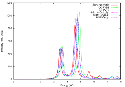
Figure 7.2: Optical absorption in Mg₂ calculated using various Gaussian contracted basis sets.

7.1.2 Size of the CI Expansion

The electron correlation effects, both in ground state as well as excited states, were taken into account in our calculations by inclusion of relevant configurations in the reference space of MRSDCI expansion. Larger the reference configuration space, larger will be the CI expansion, which is prohibitive for bigger systems. A good chemical accuracy is obtained by moderately sized CI expansion. In Table 7.1 we present the average number of reference states (N_ref) included in the MRSDCI expansion and average number of configurations (N_total) for different isomers. For a given isomer, the average has been calculated across different irreducible representations needed in the calculations in order to compute the ground and various excited states. The extensiveness of our calculations can be seen from the number N_total, which is $\approx$ 45000 for the simplest cluster, and around three million for each symmetry subspace of Mg₅.

Before we discuss the absorption spectrum for each isomer, we present the ground state energies along with the relative energies of each isomer are given in Table 7.1.

Table 7.1: The average number of reference configurations (N_ref), and average number of total configurations (N_total) involved in MRSDCI calculations, ground state (GS) energies (in Hartree) at the MRSDCI level, relative energies and correlation energies (in eV) of various isomers of magnesium clusters.

Cluster	Isomer	Nref	Ntotal	GS energy	Relative
				(Ha)	energy (eV)
Mg2	Linear	11	44796	-399.2847413	0.00
Mg3	Equilateral Triangular	30	239465	-598.9270344	0.00
	Linear	55	460187	-598.8759291	1.39
	Isosceles Triangular-1	34	516337	-598.8569875	1.91
	Isosceles Triangular-2	32	359780	-598.8093768	3.20
Mg4	Pyramidal	32	2962035	-798.5781385	0.00
	Rhombus	29	1278632	-798.5405148	1.02
	Square	35	1319301	-798.5278160	1.37
Mg5	Bipyramidal	11	3242198	-998.2044402	0.00
	Pyramidal	28	2215749	-998.1980062	0.18

• Full Configuration Interaction calculation performed for Mg dimer.

7.2 MRSDCI Photoabsorption Spectra of Magnesium Clusters

Next we present and discuss the results of our photoabsorption calculations for each isomer.

7.2.1 Mg₂

The simplest cluster of magnesium is Mg₂ with D_∞h point group symmetry. We obtained its CCSD optimized bond length to be 3.93 Å (cf. Fig. 7.1LABEL:sub@subfig:subfig-mg2), which is in excellent agreement with the experimental value 3.89 Å.^{180, 182} Using a DFT based methodology, several other theoretical values reported are in excellent agreement with our optimized bond length of magnesium dimer, i.e., Kumar and Car reported dimer bond length to be 3.88 Å ¹⁸¹ using density functional molecular dynamics with simulated annealing, Janecek et al. computed bond length to be 3.70 Ź⁹¹ using DFT with LDA approximation, 3.8 Å bond length was reported by Stevens and Krauss using multi-configuration self-consistent field approach¹⁸³, 3.91 Å bond length of dimer was computed by Jellinek and Acioli using DFT with BP86 exchange-correlation functional¹⁸⁴ and Lyalin et al. reported 3.926 Å bond length using DFT with B3LYP exchange-correlation functional¹⁸⁷.

The computed photoabsorption spectra of Mg₂, as shown in Fig. 7.3, is characterized couple of intense peaks in the 3 – 5 eV range and by weaker absorption at higher energies. The many-particle wavefunctions of excited states contributing to the peaks are presented in Table LABEL:Tab:table_mg2_lin. The first peak at 3.46 eV with absorption due to longitudinally polarized absorption is characterized by $H\rightarrow L+1$ followed by a weaker absorption at 4 eV characterized by a transverse polarized $H\rightarrow L+8$. The most intense peak occurs at 4.6 eV with dominant contribution from $H-1\rightarrow L$ and $H\rightarrow L+3$. This peak is also observed in the experimental photoabsorption spectrum at 4.62 eV ¹⁸². All these states exhibit strong mixing of singly-excited configurations. The wavefunctions of the excited states contributing to all the peaks exhibit strong configuration mixing, instead of being dominated by single configurations, pointing to the plasmonic nature of the optical excitations.¹²⁶

The spectrum calculated using TDDFT by Solov’yov et al.¹⁸⁹ is in excellent agreement with our results. In their calculations, first peak is seen at 3.3 eV followed by the most intense peak at 4.6 eV. The overall photoabsorption profile is also in accordance with our results.

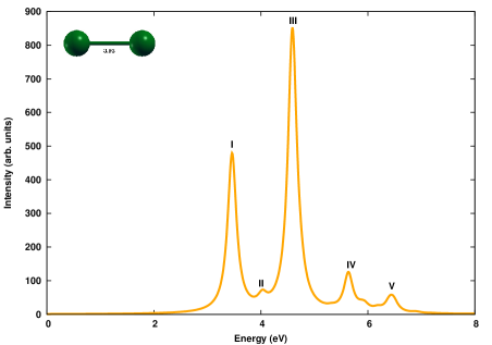
Figure 7.3: The linear optical absorption spectrum of Mg₂, calculated using the MRSDCI approach. For plotting the spectrum, a uniform linewidth of 0.1 eV was used.

7.2.2 Mg₃

We have optimized four low-lying geometries of magnesium trimer. The lowest energy structure at CCSD optimized level has equilateral triangular shape with D_3h symmetry and bond lengths of 3.48 Å. This is in good agreement with other theoretical results reported, 3.51 Å ¹⁹¹, 3.48 Å ¹⁸⁴, and 3.475 Å ¹⁸⁷. The next low-lying isomer of magnesium trimer is linear with D_∞h symmetry. The optimized bond length is found to be 2.92 Å. The remaining two low-lying isomers have isosceles triangular shape, with C_2v point group symmetry. Not much has yet been reported on the bond lengths and electronic structure of these isomers.

The photoabsorption spectra of these isomers are presented in Figs. 7.4, 7.5, 7.6 and 7.7. The corresponding many-body wavefunctions of excited states corresponding to various peaks are presented in Table LABEL:Tab:table_mg3_equil, LABEL:Tab:table_mg3_lin, LABEL:Tab:table_mg3_iso1 and LABEL:Tab:table_mg3_iso2 respectively. In the equilateral triangular isomer, bulk of the oscillator strength carried by peak at 3.7 eV. The absorption spectrum of linear isomer is altogether different with a number of peaks spread out in wide energy range, and, due to the polarization of light absorbed both parallel and perpendicular the axis of the trimer. On contrary, most of the oscillator strength in the absorption spectrum of isosceles triangular isomer-I is carried in the range of 3 – 5 eV. The spectrum of isosceles triangular isomer-II shows a slightly red shifted with respect to the isosceles isomer-I, while peaks are observed in the entire ultraviolet range.

The optical absorption spectrum of equilateral triangular isomer consists of a weaker absorption peak at 2.6 eV characterized by $H\rightarrow L$ and $H\rightarrow L+4$. This is followed by the most intense peak at 3.7 eV due to the light polarized both parallel and perpendicular to the plane of the isomer, and with dominant contribution from $H\rightarrow L$, $H\rightarrow L+2$ and $H-1\rightarrow L$. This is confirmed by an experimental result of photoabsorption of Mg trimer in argon matrix, which shows a peak at 3.64 eV. ¹⁸² Semi-major peaks at around 4.7 eV and 5.8 eV get dominant contribution from $H\rightarrow L+7$, $H\rightarrow L+5$ and $H\rightarrow L+9$ configurations. The latter being characterized by light polarized perpendicular to the plane of isomer.

Comparing our results with the spectrum obtained by TDDFT calculations¹⁸⁹, we see a good agreement on overall profile of spectrum and excitation energies. First peak is observed at 2.5 eV followed by most intense one at 3.7 eV in the TDDFT spectrum. Excitation energies and relative oscillator strengths are also in good agreement with our results.

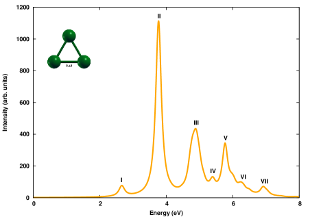
Figure 7.4: The linear optical absorption spectrum of Mg₃ equilateral triangle isomer, calculated using the MRSDCI approach. For plotting the spectrum, a uniform linewidth of 0.1 eV was used.

Because the ground state of Mg₃ linear isomer is a spin triplet, its many-particle wavefunction predominantly consists of a configuration with two degenerate singly occupied molecular orbitals referred to as $H_{1}$ and $H_{2}$ in rest of the discussion. Naturally, the excited state wavefunctions will consist of configurations involving electronic excitations from the occupied MOs (including singly occupied) to the unoccupied MOs starting from LUMO. Linear trimer of magnesium cluster records absorption in the entire energy range. Very feeble peaks are observed at 0.9 eV and 2.3 eV, characterized by $H_{1}\rightarrow L+8$ and $H_{1}\rightarrow L+4$ respectively. The semi-major peak at 2.9 eV get dominant contribution from $H_{1}\rightarrow L+3$. The most intense peak at 5.4 eV has almost equal contribution from $H-2\rightarrow L$ and $H-1\rightarrow L+2$. The absorption due to light polarized along the trimer contributes to the lower energy part of the spectrum, while light polarized perpendicular to the trimer contributes to the remaining higher energy part of the spectrum.

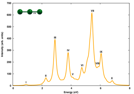
Figure 7.5: The linear optical absorption spectrum of Mg₃ linear isomer, calculated using the MRSDCI approach. For plotting the spectrum, a uniform linewidth of 0.1 eV was used.

Both isosceles triangular isomers have a spin triplet ground state, hence their excited state wavefunctions will consist of configurations involving electronic excitations from singly occupied $H_{1}$ and $H_{2}$ molecular orbitals, in addition to other doubly occupied orbitals. In the case of isosceles triangular isomer - I, the spectrum starts with a very feeble peak at 1.1 eV with contribution from $H_{1}\rightarrow L+1$ configuration. However, most of the absorption takes place in the energy range of 3 – 5 eV, with two equally intense peaks at 3.4 eV and 4.2 eV. The former is characterized by $H-2\rightarrow L$, $H_{1}\rightarrow L+3$ and $H-1\rightarrow L+1$. The wavefunctions of excited states corresponding to most of the peaks show a strong mixing of doubly-excited configurations, as is the case with the strongest peak at 4.2 eV.

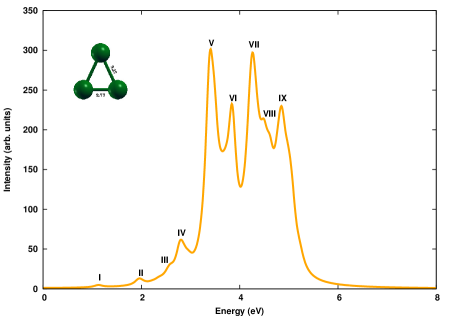
Figure 7.6: The linear optical absorption spectrum of Mg₃ isosceles triangle isomer-I, calculated using the MRSDCI approach. For plotting the spectrum, a uniform linewidth of 0.1 eV was used.

The isosceles triangular isomer -II shows a red-shifted spectrum in comparison to the former isomer, with a distinction of well separated peaks. The most intense peak at 2.6 eV gets dominant contribution from $H_{2}\rightarrow L$ and a doubly-excited configuration $H_{2}\rightarrow L;H_{1}\rightarrow L+10$. Two almost equally intense peaks of absorption due to in-plane polarization at 3.5 eV and 3.9 eV are characterized by $H-2\rightarrow H_{1}$ configurations, along with $H_{1}\rightarrow L+7$ and $H_{1}\rightarrow L+17$ respectively. This isomer also exhibits a strong mixing of doubly-excited configurations in the excited states.

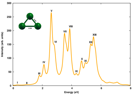
Figure 7.7: The linear optical absorption spectrum of Mg₃ isosceles triangle isomer-II, calculated using the MRSDCI approach. For plotting the spectrum, a uniform linewidth of 0.1 eV was used.

7.2.3 Mg₄

The most stable isomer of Mg₄ cluster is a pyramidal / tetrahedron type isomer, with T_d point group symmetry and 3.22 Å optimized bond length. Previously reported bond lengths 3.09 Å ¹⁸⁰, 3.33 Å ¹⁹¹, 3.18 Å ¹⁸⁴, 3.31 Å ¹⁸⁵ and 3.32 Å ¹⁸⁶ are in very good agreement with our results. The rhombus isomer with D_2h point group symmetry lies 1.02 eV above the global minimum structure. The optimized bond length is 3.0 Å with acute angle of 63.5. Square isomer with D_4h point group symmetry and ${}^{3}B_{2u}$ electronic ground state lies 1.37 eV from the most stable structure.

The absorption spectra of pyramidal, rhombus and square isomers are presented in Figs. 7.8, 7.9, and 7.10 respectively and many-particle wavefunctions of excited states contributing to various peaks are presented in Table LABEL:Tab:table_mg4_pyra, LABEL:Tab:table_mg4_rho and LABEL:Tab:table_mg4_sqr respectively. The onset of absorption spectrum of pyramidal isomer is seen at 2.6 eV with dominant contribution coming from $H-1\rightarrow L$, $H\rightarrow L$ and $H-2\rightarrow L$ configurations. The absorption spectrum of pyramidal isomer shows a very strong absorption at 4.5 eV due to light polarized in all three directions. It is exhibited by $H\rightarrow L+2$, $H-1\rightarrow L+1$ etc. electronic excitations.

The TDDFT absorption spectrum reported by Solov’yov et al.¹⁸⁹, is slightly red-shifted, however its absorption pattern is similar compared to our calculated spectrum. A single most intense peak is seen at 4.2 eV followed by several less intense peaks.

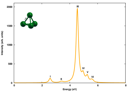
Figure 7.8: The linear optical absorption spectrum of pyramidal Mg₄ isomer, calculated using the MRSDCI approach. For plotting the spectrum, a uniform linewidth of 0.1 eV was used.

In case of rhombus isomer, the bulk of the oscillator strength is distributed in the energy range 4 – 6 eV. Several equally intense and closely-lying peaks are observed in this range. The most intense peak, at 4.7 eV, is characterized by $H-1\rightarrow L+1$ along with its shoulder at 4.6 eV, which gets dominant contribution from $H_{2}\rightarrow L+8$. Both are due to light polarized in the plane of the isomer.

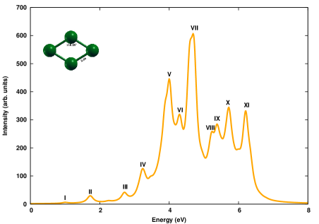
Figure 7.9: The linear optical absorption spectrum of rhombus Mg₄, calculated using the MRSDCI approach. For plotting the spectrum, a uniform linewidth of 0.1 eV was used.

The absorption spectrum of the square structure is slightly blue-shifted as compared to the rhombus and red-shifted as compared to pyramidal isomer, with the majority of absorption occurring in the energy range 3–6 eV. The onset of absorption spectrum occurs at 1.5 eV with peak due to light polarized in the plane of isomer, and characterized by $H_{1}\rightarrow L+15$ and $H_{1}\rightarrow L+10$. Square isomer also exhibits two very closely spaced most intense peaks, as is observed in rhombus counterpart. These peaks at 4.5 eV and 4.7 eV have contribution from singly-excited configurations such as $H-1\rightarrow L$ and $H_{1}\rightarrow L+24$ respectively as well as doubly-excited configurations.

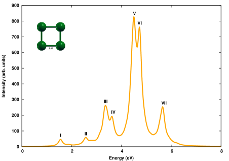
Figure 7.10: The linear optical absorption spectrum of square Mg₄, calculated using the MRSDCI approach. For plotting the spectrum, a uniform linewidth of 0.1 eV was used.

7.2.4 Mg₅

We optimized geometries of two isomers of Mg₅: (a) bipyramid with the D_3h symmetry, and (b) a pyramidal with the C_4v point group symmetry. The lowest lying pentagon isomer, has ¹A${}_{1}^{{}^{\prime}}$ electronic ground state, and is just 0.18 eV lower in energy as compared to the pyramid structure. Our optimized geometry for the bipyramid corresponds to unique bond lengths of 3.15 Å and 3.52 Å, as against 3.00 Å, 3.33 Å reported by J. Jellinek and Acioli ¹⁸⁴; and 3.09 Å, 3.44 Å reported by Andrey et al. ¹⁸⁷

The bipyramidal isomer of Mg₅ cluster, exhibits an absorption spectrum very different from other isomers, as displayed in Fig. 7.11. The many-particle wavefunctions of excited states contributing to the peaks are presented in Table LABEL:Tab:table_mg5_biprism. The optical absorption spectrum of bipyramidal Mg₅ has no absorption until 3.5 eV, while most of the absorption takes place in a narrow energy range 5.3 – 6.3 eV. The absorption spectrum begins at 3.6 eV, with a very feeble peak with contribution from $H-1\rightarrow L+4$ configuration. This is followed by several such smaller peaks. The most intense peak at 5.4 eV has dominant contribution from $H\rightarrow L+1$ and $H-1\rightarrow L+3$ with absorption polarized along $y-$direction, which is in the plane of the triangle of the pyramid. A shoulder peak at 5.6 eV however has absorption due to light polarized along $z-$ direction, which is along the larger dimension of the isomer.

The TDDFT spectrum computed by Solov’yov et al.¹⁸⁹ shows optical activity in the energy range of 2 –4 eV, which is not observed in our calculated spectrum. However, a quasi-continuous spectrum is seen at higher energies in both calculations.

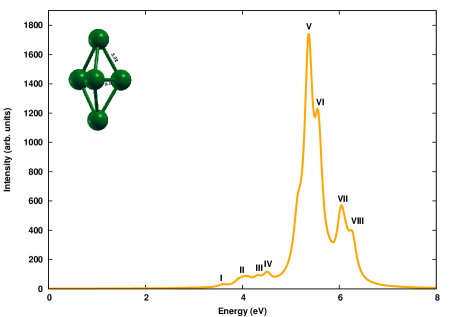
Figure 7.11: The linear optical absorption spectrum of bipyramidal Mg₅ isomer, calculated using the MRSDCI approach. For plotting the spectrum, a uniform linewidth of 0.1 eV was used.

The entire absorption spectrum of pyramidal isomer is highly red-shifted as compared to the bipyramidal isomer. A few feeble peaks occur in the low energy range in the optical absorption of pyramidal isomer. The many-particle wavefunctions of excited states contributing to the peaks are presented in Table LABEL:Tab:table_mg5_param. The onset of spectrum occurs at 2.2 eV with absorption due to polarization both perpendicular as well as in the plane of base of pyramid. It is characterized by $H-1\rightarrow L$ and $H\rightarrow L+2$. An intense peak at 3.5 eV separates itself from the most intense one at 4.2 eV. The former gets dominant contribution from $H-1\rightarrow L+3$ and $H-2\rightarrow L$ configurations. While the most intense peak is due to light polarized perpendicular to the basal plane of pyramid, and contributed from $H-2\rightarrow L+1$ and $H-2\rightarrow L+3$. Pyramidal isomer shows more optical absorption in the high energy range, with peaks within regular intervals of energy with declining intensities, in contrast to single major peak observed in the spectrum of bipyramidal isomer. These differences can lead to identification of isomers produced experimentally.

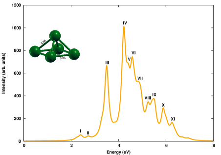
Figure 7.12: The linear optical absorption spectrum of pyramidal Mg₅, calculated using the MRSDCI approach. For plotting the spectrum, a uniform linewidth of 0.1 eV was used.

7.3 Summary

we have presented large-scale all-electron correlated calculations of optical absorption spectra of several low-lying isomers of magnesium clusters Mg_n, (n=2–5). We computed the ground state and excited states of magnesium dimer using one of the best possible electronic structure methods, namely full configuration interaction with frozen-core approximation. In case of remaining clusters, both ground and excited state calculations were performed at MRSDCI level, which take electron correlations into account at a sophisticated level. We have analyzed the nature of low-lying excited states. Isomers of a given cluster show a distinct signature spectrum, indicating a strong-structure property relationship. This fact can be used in experiments to distinguish between different isomers of a cluster. Our calculations suggests that the optical excitations involved are found to be collective type because of a strong mixing of configurations, and hence are plasmonic in nature. Owing to the sophistication of our calculations, our results can be used for benchmarking of the absorption spectra as well as for designing functionals for superior TDDFT results.

Chapter 8 Conclusions and Outlook

We performed systematic large-scale all-electron correlated calculations on boron B_n, aluminum Al_n and magnesium Mg_n clusters (n=2–5), to study their linear optical absorption spectra. Several possible isomers of each cluster were considered, and their geometries were optimized at the coupled-cluster singles doubles (CCSD) level of theory. Using the optimized ground-state geometries, excited states of different clusters were computed using the multi-reference singles-doubles configuration-interaction (MRSDCI) approach, which includes electron correlation effects at a sophisticated level. These CI wavefunctions were used to compute the transition dipole matrix elements connecting the ground and various excited states of different clusters, eventually leading to their linear absorption spectra. The convergence of our results with respect to the basis sets, and the size of the CI expansion was carefully examined. Isomers of a given cluster show a distinct signature spectrum, indicating a strong-structure property relationship. This fact can be used in experiments to distinguish between different isomers of a cluster. Owing to the sophistication of our calculations, our results can be used for benchmarking of the absorption spectra and be used to design superior time-dependent density functional theoretical (TDDFT) approaches. The contribution of configurations to many-body wavefunction of various excited states suggests that in most cases optical excitations involved are collective, and plasmonic in nature.

In addition, we calculated the optical absorption in various isomers of neutral boron B₆ and cationic boron B${}_{6}^{+}$ clusters using computationally less expensive configuration interaction singles (CIS) approach, and benchmarked these results against more sophisticated equation-of-motion (EOM) CCSD based approach. In all closed shell systems, a complete agreement on the nature of configurations involved is observed in both methods. On the other hand, for open-shell systems, minor contribution from double excitations are observed, which are not captured in the CIS method.

Optical absorption in planar boron clusters in wheel shape, B₇, B₈ and B₉ computed using EOM-CCSD approach, have been compared to the results obtained from TDDFT approach with a number of functionals. Hybrid GGA functionals – PBE0, B3LYP and B3PW91 – are also poor performers as they tend to underestimate the excitations energies. Meta-GGA functionals M06 and M06-2X –which includes terms that depend on kinetic energy density – also underestimate the excitation energies. Among the long-range corrected functionals CAM-B3LYP provides the best agreement with EOM results on the basis of excitation energies as well as spectrum profile. The contribution of configurations to the many-body wavefunctions of various excited states suggest that the excitations involved are of molecular type. Since most of the absorption takes place at higher energies, these clusters could potentially be used as ultraviolet absorbers. Although this study neither includes all the functionals available nor does the test cases are comprehensive, it helps in providing reasonable comparison between the current gold standard single reference method, namely, EOM-CCSD and TDDFT, by identifying the functionals which provide results as good as EOM-CCSD in light of optical absorption calculations. These findings can be tested against more sophisticated multi-reference calculations. Such high-level calculations are necessary to design superior yet less time-consuming TDDFT approaches.

The large-scale configuration interaction based approach can be extended to study non-linear optical phenomenon in clusters, such as excited state absorption, multi-photon absorption, higher-harmonic generation etc. We also look forward to use such a sophisticated approach to study ab initio photo-emission spectra of atomic and molecular clusters.

For large and extended systems, such as, clusters of ceramic materials (BeO)_n, (Li₂O)_n and (B₂O₃)_n (n = 2 – 20) calculations of linear optical absorption using TDDFT approach are currently under consideration. Results for these systems will be communicated soon. Some of these clusters also show reversible hydrogen adsorption properties. For instance, (BeO)_n shows remarkable hydrogen adsorption, meeting US Department of Energy ultimate goal of 7.5 wt/% hydrogen adsorption. This study was performed in collaboration, whose results are now under revision.

An ab initio description of Angle-Resolved Photo-Emission Spectra (ARPES) of 2-D surfaces and 3-D bulk, using TDDFT, is also under consideration. This will help enormously in explaining the experimental ARPES spectra, which are usually obtained for bulk or 2-D samples.

Appendix A Boron Clusters B_n (n = 2 – 5)

In the following tables, we have given the excitation energies (with respect to the ground state), and the many-body wavefunctions of the excited states, corresponding to the peaks in the MRSDCI photoabsorption spectra of various boron cluster isomers listed in Fig. 3.1, and discussed in Chapter 3. along with the oscillator strength $f_{12}$ of the transitions,

$$f_{12}=\frac{2}{3}\frac{m_{e}}{\hbar^{2}}(E_{2}-E_{1})\sum_{i}|\langle m|d_{i}|G\rangle|^{2}$$ (A.1)

where, $|m\rangle$ denotes the excited state in question, $|G\rangle$, the ground state, and $d_{i}$ is the $i$-th Cartesian component of the electric dipole operator. The single excitations are with respect to the reference state as given in respective tables.

Excited State CI Wavefunctions, Energies and Oscillator Strengths

Table A.1: Excitation energies, $E$, and many-particle wavefunctions of excited states corresponding to the peaks in the linear absorption spectrum of B₂ (cf. Fig. 3.5), along with the oscillator strength of the transitions. Longitudinal and transverse polarization corresponds to the absorption due to light polarized along and perpendicular to the molecular axis respectively. In the wavefunction, the bracketed numbers are the CI coefficients of a given electronic configuration. Symbols $H_{1}$,$H_{2}$ denote SOMOs discussed earlier, and $H$, and $L$, denote HOMO and LUMO orbitals respectively. $HF$ denotes the Hartree-Fock configuration.

Peak	$E$ (eV)	$f_{12}$	Pol.	Wave Function
GSa				$|HF\rangle$ (0.8673)
				$|H-1\rightarrow L;H-1\rightarrow L\rangle$(0.2706)
				$|H-1\rightarrow L;H-1\rightarrow L+4\rangle$(0.1283)
I	0.845	0.0156	transverse	$|H_{2}\rightarrow L\rangle$(0.8742)
				$|H_{2}\rightarrow L+4\rangle$(0.2194)
II	4.207	0.1463	longitudinal	$|H-1\rightarrow L\rangle$(0.7599)
				$|H_{1}\rightarrow L+7\rangle$(0.2873)
				$|H_{2}\rightarrow L+7\rangle$(0.2873)
III	4.914	0.0558	transverse	$|H-1\rightarrow L;H-1\rightarrow L+2\rangle$(0.7553)
				$|H-2\rightarrow L+2\rangle$(0.3186)
				$|H-1\rightarrow L+7\rangle$(0.266)
IV	6.97	0.5651	transverse	$|H_{2}\rightarrow L+4\rangle$(0.5600)
				$|H_{2}\rightarrow L+5\rangle$(0.5150)
	7.05	2.3743	longitudinal	$|H-1\rightarrow L\rangle$(0.4462)
				$|H_{2}\rightarrow L+3\rangle$(0.3346)
				$|H_{1}\rightarrow L+3\rangle$(0.3346)
				$|H-1\rightarrow L+4\rangle$(0.2921)
V	7.973	0.0906	longitudinal	$|H-1\rightarrow L;H_{2}\rightarrow L+2\rangle$(0.5613)
				$|H-1\rightarrow L;H_{1}\rightarrow L+2\rangle$(0.5613)
				$|H-1\rightarrow L+4\rangle$(0.2303)

Table A.2: Excitation energies, $E$, and many-particle wavefunctions of excited states corresponding to the peaks in the linear absorption spectrum of triangular B₃ (cf. Fig. 3.6), along with oscillator strength of transition. The polarization $\|$ corresponds to the absorption due to light polarized in the plane of isomer, while $\bot$ corresponds to the polarization perpendicular to that plane. In the wavefunction, the bracketed numbers are the CI coefficients of a given electronic configuration. Symbol $L$ and $H$ denote LUMO and SOMO orbitals discussed earlier. $HF$ denotes the Hartree-Fock configuration.

Peak	$E$ (eV)	$f_{12}$	Pol.	Wave Function
GSa				$|HF\rangle$ (0.8229)
				$|H-3\rightarrow L\rangle$(0.2162)
				$|H\rightarrow L\rangle$(0.2072)
				$|H-3\rightarrow H\rangle$(0.1544)
I	0.797	0.0119	$\bot$	$|H-1\rightarrow H\rangle$(0.7357)
				$|H-1\rightarrow L\rangle$(0.4693)
				$|H-1\rightarrow L+8\rangle$(0.1142)
II	1.710	0.0035	$\|$	$|H\rightarrow L+1\rangle$(0.4816)
				$|H-2\rightarrow H\rangle$(0.4315)
				$|H-2\rightarrow L\rangle$(0.3757)
				$|H-3\rightarrow L+1\rangle$(0.3709)
		0.0037	$\|$	$|H\rightarrow L\rangle$(0.5041)
				$|H-3\rightarrow H\rangle$(0.4703)
III	2.840	0.0679	$\|$	$|H-2\rightarrow H\rangle$(0.5374)
				$|H\rightarrow L+1\rangle$(0.5199)
				$|H-2\rightarrow L\rangle$(0.3306)
				$|H-3\rightarrow L+1\rangle$(0.2216)
	2.872	0.0622	$\|$	$|H\rightarrow L\rangle$(0.4906)
				$|H-3\rightarrow L\rangle$(0.4499)
IV	5.710	0.0428	$\|$	$|H-2\rightarrow L\rangle$(0.4114)
				$|H-2\rightarrow H\rangle$(0.3474)
	5.730	0.0269	$\|$	$|H-3\rightarrow L\rangle$(0.4202)
				$|H-2\rightarrow H;H-3\rightarrow L\rangle$(0.2050)
V	5.988	0.0663	$\|$	$|H-3\rightarrow L+1\rangle$(0.3968)
				$|H-2\rightarrow L\rangle$(0.3057)
				$|H-2\rightarrow H\rangle$(0.1578)
	6.02	0.1270	$\|$	$|H-3\rightarrow L\rangle$(0.2578)
				$|H\rightarrow L\rangle$(0.1908)
VI	7.657	0.2151	$\|$	$|H\rightarrow L+2\rangle$(0.5863)
				$|H-3\rightarrow L+2\rangle$(0.2497)
				$|H\rightarrow L+14\rangle$(0.2431)
				$|H\rightarrow L+4\rangle$(0.2093)
	7.697	0.1409	$\|$	$|H\rightarrow L+3\rangle$(0.2991)
				$|H-3\rightarrow L+1\rangle$(0.2648)
				$|H-2\rightarrow H\rangle$(0.1794)
				$|H-2\rightarrow L\rangle$(0.1521)
VII	7.893	0.2797	$\bot$	$|H\rightarrow L+5\rangle$(0.7611)
				$|H-3\rightarrow L+4\rangle$(0.3477)

Table A.3: Excitation energies, $E$, and many-particle wavefunctions of excited states corresponding to the peaks in the linear absorption spectrum of linear B₃ (cf. Fig. 3.7), along with oscillator strength of transition. Longitudinal and transverse polarization corresponds to the absorption due to light polarized along and perpendicular to the molecular axis respectively. In the wavefunction, the bracketed numbers are the CI coefficients of a given electronic configuration. Symbols $H$ and $L$ denote HOMO and LUMO orbitals respectively, and $H_{1}$ denotes SOMOs discussed earlier. $HF$ denotes the Hartree-Fock configuration.

Peak	$E$ (eV)	$f_{12}$	Pol.	Wave Function
GSa				$|HF\rangle$ (0.6650)
				$|H-1\rightarrow L;H-1\rightarrow L\rangle$(0.3286)
				$|H-1\rightarrow L;H-1\rightarrow L\rangle$(0.3277)
				$|H\rightarrow L;H-1\rightarrow L+1\rangle$(0.2158)
				$|H\rightarrow L;H-1\rightarrow L+1\rangle$(0.2157)
I	0.723	0.0199	longitudinal	$|H\rightarrow L\rangle$(0.8222)
II	2.707	0.0175	transverse	$|H-1\rightarrow L\rangle$(0.5360)
III	4.338	0.5930	longitudinal	$|H-1\rightarrow L;H-1\rightarrow H\rangle$(0.5826)
				$|H-1\rightarrow L;H-1\rightarrow H\rangle$(0.5826)
IV	5.937	0.0301	longitudinal	$|H-2\rightarrow L\rangle$(0.2497)
V	7.359	1.1053	longitudinal	$|H-1\rightarrow L+1\rangle$(0.3683)
				$|H-1\rightarrow L+1\rangle$(0.3683)
				$|H-3\rightarrow L;H\rightarrow L\rangle$(0.3301)
				$|H-3\rightarrow H\rangle$(0.2364)
VI	7.731	0.3921	longitudinal	$|H-2\rightarrow L\rangle$(0.3858)
				$|H\rightarrow L;H-1\rightarrow L+4\rangle$(0.2851)
				$|H\rightarrow L;H-1\rightarrow L+4\rangle$(0.2851)
	7.786	0.3062	transverse	$|H-1\rightarrow L;H-1\rightarrow L+4\rangle$(0.6438)
				$|H-1\rightarrow L;H-1\rightarrow L+4\rangle$(0.3905)

Table A.4: Excitation energies, $E$, and many-particle wavefunctions of excited states corresponding to the peaks in the linear absorption spectrum of rhombus B₄ (cf. Fig. 3.8), along with oscillator strength of transition. The polarization in-plane corresponds to the absorption due to light polarized in the plane of isomer. In the wavefunction, the bracketed numbers are the CI coefficients of a given electronic configuration. Symbols $H$/$L$ denote HOMO/LUMO orbitals. $HF$ denotes the Hartree-Fock configuration.

Peak	$E$ (eV)	$f_{12}$	Pol.	Wave Function
GSa				$|HF\rangle$ (0.8787)
				$|H\rightarrow L;H\rightarrow L\rangle$(0.1147)
I	4.159	0.4684	in-plane	$|H\rightarrow L+2\rangle$(0.6566)
				$|H\rightarrow L+10\rangle$(0.3210)
				$|H-1\rightarrow L+6\rangle$(0.2773)
				$|H-1\rightarrow L+17\rangle$(0.1850)
II	6.118	0.3925	in-plane	$|H-1\rightarrow L+6\rangle$(0.5786)
				$|H-1\rightarrow L+17\rangle$(0.3285)
				$|H-3\rightarrow L\rangle$(0.2656)
				$|H-2\rightarrow L+11\rangle$(0.2544)
				$|H-2\rightarrow L+18\rangle$(0.2492)
III	6.639	0.0490	in-plane	$|H-1\rightarrow L+3\rangle$(0.4496)
				$|H-1\rightarrow L+13\rangle$(0.4485)
				$|H-4\rightarrow L\rangle$(0.4052)
				$|H\rightarrow L+11\rangle$(0.2766)
				$|H\rightarrow L+1\rangle$(0.2329)
				$|H\rightarrow L+18\rangle$(0.1905)
IV	7.311	0.2528	in-plane	$|H\rightarrow L+2\rangle$(0.3055)
				$|H-2\rightarrow L+11\rangle$(0.2892)
				$|H-3\rightarrow L\rangle$(0.2834)
				$|H-2\rightarrow L+18\rangle$(0.2487)
				$|H-2\rightarrow L+1\rangle$(0.2029)
				$|H-2\rightarrow L+5\rangle$(0.1509)
V	7.842	0.3951	in-plane	$|H\rightarrow L+2\rangle$(0.4233)
				$|H\rightarrow L+10\rangle$(0.3270)
				$|H-2\rightarrow L+11\rangle$(0.2049)
				$|H\rightarrow L+20\rangle$(0.1946)
				$|H-2\rightarrow L+1\rangle$(0.1594)
				$|H-2\rightarrow L+18\rangle$(0.1582)

Table A.5: Excitation energies, $E$, and many-particle wavefunctions of excited states corresponding to the peaks in the linear absorption spectrum of square B₄ (cf. Fig. 3.9), along with oscillator strength of transition. The polarization in-plane corresponds to the absorption due to light polarized in the plane of isomer. In the wavefunction, the bracketed numbers are the CI coefficients of a given electronic configuration. Symbols $H$/$L$ denote HOMO/LUMO orbitals. $HF$ denotes the Hartree-Fock configuration.

Peak	$E$ (eV)	$f_{12}$	Pol.	Wave Function
GSa				$|HF\rangle$ (0.8682)
				$|H\rightarrow L;H\rightarrow L\rangle$(0.1765)
				$|H-2\rightarrow L;H-2\rightarrow L\rangle$(0.0920)
I	4.879	0.5678	in-plane	$|H\rightarrow L;H\rightarrow L+1\rangle$(0.2946)
				$|H\rightarrow L;H-3\rightarrow L\rangle$(0.1909)
				$|H-2\rightarrow L;H-3\rightarrow L\rangle$(0.1651)
II	5.462	0.0235	in-plane	$|H\rightarrow L;H\rightarrow L+1\rangle$(0.5893)
				$|H\rightarrow L;H\rightarrow L+6\rangle$(0.2477)
III	6.418	0.2842	in-plane	$|H\rightarrow L;H-3\rightarrow L\rangle$(0.5379)
				$|H\rightarrow L;H\rightarrow L+1\rangle$(0.2922)
				$|H-2\rightarrow L;H-3\rightarrow L\rangle$(0.1744)
IV	7.890	1.3888	in-plane	$|H\rightarrow L+1;H-1\rightarrow L\rangle$(0.2351)

Table A.6: Excitation energies, $E$, and many-particle wavefunctions of excited states corresponding to the peaks in the linear absorption spectrum of linear B₄ (cf. Fig. 3.10), along with oscillator strength of transition. Longitudinal and transverse polarization corresponds to the absorption due to light polarized along and perpendicular to the molecular axis respectively. In the wavefunction, the bracketed numbers are the CI coefficients of a given electronic configuration. Symbols $H$/$L$ denote HOMO/LUMO orbitals. $HF$ denotes the Hartree-Fock configuration.

Peak	$E$ (eV)	$f_{12}$	Pol.	Wave Function
GSa				$|HF\rangle$ (0.5636)
				$|H\rightarrow L\rangle$(0.4737)
				$|H-1\rightarrow L;H\rightarrow L+1\rangle$(0.2291)
				$|H-1\rightarrow L;H\rightarrow L+1\rangle$(0.2289)
I	5.363	0.0976	longitudinal	$|H\rightarrow L;H-1\rightarrow L+9\rangle$(0.3005)
				$|H\rightarrow L;H-1\rightarrow L+9\rangle$(0.3005)
				$|H\rightarrow L;H-1\rightarrow L+8\rangle$(0.2702)
				$|H\rightarrow L;H-1\rightarrow L+8\rangle$(0.2702)
				$|H\rightarrow L;H-1\rightarrow L+4\rangle$(0.2439)
				$|H\rightarrow L;H-1\rightarrow L+4\rangle$(0.2439)
II	5.947	4.1752	longitudinal	$|H-1\rightarrow L+1\rangle$(0.2957)
				$|H-1\rightarrow L+1\rangle$(0.2957)
III	7.352	1.8444	longitudinal	$|H\rightarrow L;H-2\rightarrow L\rangle$(0.6477)
				$|H-3\rightarrow L\rangle$(0.2966)
				$|H-1\rightarrow L+1\rangle$(0.2091)
				$|H-1\rightarrow L+1\rangle$(0.2091)
	7.380	1.0202	transverse	$|H-1\rightarrow L+13\rangle$(0.5253)

Table A.7: Excitation energies, $E$, and many-particle wavefunctions of excited states corresponding to the peaks in the linear absorption spectrum of distorted tetrahedron B₄ (cf. Fig. 3.11), along with oscillator strength of transition. The polarization $x$,$y$ and $z$ corresponds to the absorption due to light polarized along $x-$,$y-$ and $z-$ axis respectively. In the wavefunction, the bracketed numbers are the CI coefficients of a given electronic configuration. Symbols $H$/$L$ denote HOMO/LUMO orbitals. $HF$ denotes the Hartree-Fock configuration.

Peak	$E$ (eV)	$f_{12}$	Pol.	Wave Function
GSa				$|HF\rangle$ (0.6493)
				$|H\rightarrow L;H\rightarrow L+2\rangle$(0.4695)
				$|H\rightarrow L;H-3\rightarrow L+2\rangle$(0.1547)
I	1.000	0.0068	x	$|H\rightarrow L\rangle$(0.8127)
				$|H\rightarrow L;H-1\rightarrow L+2\rangle$(0.2364)
	1.111	0.0094	y	$|H\rightarrow L+2;H\rightarrow L+1\rangle$(0.5944)
				$|H\rightarrow L;H\rightarrow L+1\rangle$(0.5121)
II	3.609	0.0364	x	$|H\rightarrow L;H-1\rightarrow L+2\rangle$(0.5094)
				$|H\rightarrow L;H-1\rightarrow L\rangle$(0.4535)
				$|H\rightarrow L+2\rangle$(0.3480)
	3.754	0.0519	y	$|H\rightarrow L+1;H\rightarrow L+2\rangle$(0.2391)
III	4.48	0.0632	z	$|H-1\rightarrow L\rangle$(0.4418)
IV	4.96	0.0767	z	$|H-1\rightarrow L\rangle$(0.2678)
				$|H\rightarrow L;H-3\rightarrow L\rangle$(0.2227)
V	5.92	0.0913	x	$|H-3\rightarrow L\rangle$(0.2191)
				$|H\rightarrow L+2;H-4\rightarrow L\rangle$(0.2191)
VI	6.15	0.0895	y	$|H\rightarrow L;H-3\rightarrow L+1\rangle$(0.2526)
VII	6.508	0.0159	z	$|H-1\rightarrow L+2\rangle$(0.7131)
				$|H-1\rightarrow L\rangle$(0.2104)
				$|H\rightarrow L+2;H\rightarrow L+2\rangle$(0.2030)
VIII	6.858	0.1881	x	$|H\rightarrow L;H\rightarrow L+10\rangle$(0.6912)
				$|H\rightarrow L+2;H\rightarrow L+10\rangle$(0.3415)
				$|H\rightarrow L+18;H\rightarrow L\rangle$(0.2759)
	6.99	0.1488	y	$|H\rightarrow L;H\rightarrow L+5\rangle$(0.4169)
				$|H\rightarrow L+2;H\rightarrow L+5\rangle$(0.3770)
				$|H\rightarrow L+3;H-1\rightarrow L\rangle$(0.2403)
				$|H-1\rightarrow L+1\rangle$(0.2156)
IX	7.80	0.0686	z	$|H-1\rightarrow L;H-1\rightarrow L+2\rangle$(0.3386)
				$|H\rightarrow L;H-4\rightarrow L+2\rangle$(0.3164)
				$|H\rightarrow L;H-4\rightarrow L+2\rangle$(0.2987)
				$|H-1\rightarrow L;H-1\rightarrow L\rangle$(0.2722)
				$|H\rightarrow L+1;H-1\rightarrow L+3\rangle$(0.2174)

Table A.8: Excitation energies, $E$, and many-particle wavefunctions of excited states corresponding to the peaks in the linear absorption spectrum of pentagon B₅ (cf. Fig. 3.12), along with oscillator strength of transition. The polarization in-plane corresponds to the absorption due to light polarized in the plane of isomer. In the wavefunction, the bracketed numbers are the CI coefficients of a given electronic configuration. Symbols $H$ and $L$ denote HOMO and LUMO orbitals respectively. $HF$ denotes the Hartree-Fock configuration.

Peak	$E$ (eV)	$f_{12}$	Pol.	Wave Function
GSa				$|HF\rangle$ (0.8541)
				$|H-1\rightarrow L\rangle$(0.1906)
I	1.394	0.0237	$\bot$ to the plane	$|H\rightarrow L+1\rangle$(0.8536)
				$|H\rightarrow L+11\rangle$(0.1779)
II	1.818	0.0096	in-plane	$|H\rightarrow L\rangle$(0.6524)
				$|H-1\rightarrow H\rangle$(0.4900)
				$|H\rightarrow L+3\rangle$(0.2218)
III	3.504	0.0848	in-plane	$|H-2\rightarrow L+1\rangle$(0.5804)
				$|H-1\rightarrow H\rangle$(0.5131)
				$|H\rightarrow L\rangle$(0.3441)
IV	3.868	0.0372	in-plane	$|H-2\rightarrow L+1\rangle$(0.7968)
				$|H-1\rightarrow H\rangle$(0.3416)
V	4.379	0.0247	in-plane	$|H-3\rightarrow H\rangle$(0.8185)
				$|H-4\rightarrow L\rangle$(0.1900)
VI	5.378	0.1642	in-plane	$|H-1\rightarrow L\rangle$(0.7309)
				$|H-4\rightarrow L\rangle$(0.3583)
				$|H-1\rightarrow L+3\rangle$(0.1994)
				$|H-3\rightarrow H\rangle$(0.1808)
	5.576	0.6640	in-plane	$|H-2\rightarrow L+1\rangle$(0.4415)
				$|H-3\rightarrow L\rangle$(0.4045)
				$|H-4\rightarrow H\rangle$(0.4000)
				$|H\rightarrow L\rangle$(0.2399)
				$|H-1\rightarrow L+4\rangle$(0.2039)
VII	6.305	0.6453	in-plane	$|H-3\rightarrow L\rangle$(0.4073)
				$|H-1\rightarrow L+4\rangle$(0.3328)
				$|H-1\rightarrow L+9\rangle$(0.2952)
				$|H-2\rightarrow L+1\rangle$(0.2870)
				$|H-4\rightarrow L+4\rangle$(0.2772)
				$|H-4\rightarrow L+9\rangle$(0.2531)
	6.528	0.1049	in-plane	$|H-1\rightarrow L\rangle$(0.5596)
				$|H-4\rightarrow L\rangle$(0.3400)
				$|H-2\rightarrow L+2\rangle$(0.2761)
				$|H-3\rightarrow L+4\rangle$(0.2667)
				$|H-3\rightarrow L+9\rangle$(0.2598)
VIII	7.161	0.2561	in-plane	$|H-4\rightarrow L+4\rangle$(0.4305)
				$|H-4\rightarrow L+9\rangle$(0.3859)
				$|H-3\rightarrow L\rangle$(0.3776)
				$|H-1\rightarrow L+4\rangle$(0.2487)
	7.283	0.0781	in-plane	$|H\rightarrow L+6\rangle$(0.7102)
				$|H\rightarrow L+9\rangle$(0.3359)
				$|H-3\rightarrow L+4\rangle$(0.2091)
				$|H-3\rightarrow L+9\rangle$(0.1854)
IX	7.702	0.1345	$\bot$ to the plane	$|H\rightarrow L+11\rangle$(0.7980)
				$|H\rightarrow L+14\rangle$(0.2692)
	7.750	0.1150	in-plane	$|H-1\rightarrow L+3\rangle$(0.8332)
				$|H-1\rightarrow L+19\rangle$(0.1555)

Table A.9: Excitation energies, $E$, and many-particle wavefunctions of excited states corresponding to the peaks in the linear absorption spectrum of distorted triangular-bipyramid B₅ (cf. Fig. 3.13), along with oscillator strength of transition. The polarization $x$,$y$ and $z$ corresponds to the absorption due to light polarized along $x-$,$y-$ and $z-$ axis respectively. In the wavefunction, the bracketed numbers are the CI coefficients of a given electronic configuration. Symbols $H$ and $L$ denote HOMO and LUMO orbitals respectively. $HF$ denotes the Hartree-Fock configuration.

Peak	$E$ (eV)	$f_{12}$	Pol.	Wave Function
GSa				$|HF\rangle$ (0.8615)
				$|H-1\rightarrow H\rangle$(0.2165)
				$|H-1\rightarrow H;H-1\rightarrow L\rangle$(0.1371)
				$|H-2\rightarrow H;H-1\rightarrow L\rangle$(0.1143)
I	1.774	0.0548	z	$|H-1\rightarrow L+4\rangle$(0.8689)
II	3.161	0.0763	y	$|H-2\rightarrow H\rangle$(0.8734)
				$|H-1\rightarrow H;H-1\rightarrow L\rangle$(0.2303)
III	4.274	0.0509	z	$|H-1\rightarrow L+2\rangle$(0.8666)
				$|H-1\rightarrow L+6\rangle$(0.1775)
IV	5.487	0.1949	y	$|H-1\rightarrow H;H-1\rightarrow L\rangle$(0.7812)
				$|H-2\rightarrow H\rangle$(0.2336)
				$|H-2\rightarrow H;H-1\rightarrow L\rangle$(0.2332)
V	6.408	0.1170	z	$|H-4\rightarrow H\rangle$(0.7837)
				$|H-2\rightarrow L+2\rangle$(0.3357)
				$|H-2\rightarrow H;H-1\rightarrow L+1\rangle$(0.2274)
VI	7.519	0.4523	x	$|H-2\rightarrow H;H-1\rightarrow L+2\rangle$(0.8133)
				$|H-2\rightarrow H;H-1\rightarrow L+6\rangle$(0.2669)
VII	7.744	0.0177	x	$|H-1\rightarrow L;H-1\rightarrow L+1\rangle$(0.6105)
				$|H-1\rightarrow L+4\rangle$(0.4305)
				$|H-2\rightarrow L+1\rangle$(0.2271)

Appendix B Boron Clusters B₆ and B${}_{6}^{+}$

In the following tables, we have given the excitation energies (with respect to the ground state), and the many-body wavefunctions of the excited states, corresponding to the peaks in the CIS photoabsorption spectra of various isomers listed in Fig. 4.1 and Fig. 4.15 , along with the oscillator strength $f_{12}$ of the transitions,

$$f_{12}=\frac{2}{3}\frac{m_{e}}{\hbar^{2}}(E_{2}-E_{1})\sum_{i}|\langle m|d_{i}|G\rangle|^{2}$$ (B.1)

where, $|m\rangle$ denotes the excited state in question, $|G\rangle$, the ground state, and $d_{i}$ is the $i$-th Cartesian component of the electric dipole operator. The single excitations are with respect to the reference state as given in respective tables.

Similar tables corresponding to the results of select EOM-CCSD calculations are also given below.

Excited State CIS Wavefunctions, Energies and Oscillator Strengths

Table B.1: Excitation energies, $E$, and many-particle wavefunctions of excited states corresponding to the peaks in the CIS linear absorption spectrum of B₆ – planar ring (triplet) isomer (cf. Fig. 4.2). The subscript $\|$ in the peak number denotes the absorption due to light polarized in the plane of isomer. In the wavefunction, the bracketed numbers are the CI coefficients of a given electronic configuration. Symbols $H_{1\alpha}$,$H_{2\alpha}$ denote SOMOs discussed earlier, and $H$, and $L$, denote HOMO and LUMO orbitals respectively. Note that, the reference state does not correspond to any peak, instead it represents the reference state from which singles excitations are occurring.

Peak	$E$ (eV)	$f_{12}$	$\langle S^{2}\rangle$	Wave Function
Reference				$|H_{1\alpha}^{1};H_{2\alpha}^{1}\rangle$
I∥	2.85	0.0099	3.01	$|H_{\alpha}-2\rightarrow L_{\alpha}\rangle$(0.6589)
				$|H_{1\alpha}\rightarrow L_{\alpha}\rangle$(0.6102)
II∥	3.42	0.0634	2.90	$|H_{1\alpha}\rightarrow L_{\alpha}\rangle$(0.5415)
				$|H_{\beta}\rightarrow L_{\beta}\rangle$(0.4719)
III∥	4.31	0.0306	2.78	$|H_{\beta}-1\rightarrow L_{\beta}+1\rangle$(0.7253)
				$|H_{\beta}-2\rightarrow L_{\beta}+12\rangle$(0.3011)
IV∥	4.62	0.1830	3.30	$|H_{\beta}-3\rightarrow L_{\beta}+1\rangle$(0.6176)
				$|H_{2\alpha}\rightarrow L_{\alpha}+10\rangle$(0.3007)
V∥	4.98	0.1673	2.94	$|H_{\beta}-3\rightarrow L_{\beta}+1\rangle$(0.4591)
				$|H_{\beta}-2\rightarrow L_{\beta}+16\rangle$(0.3334)
VI∥	5.89	0.3505	2.99	$|H_{\alpha}-3\rightarrow L_{\alpha}+1\rangle$(0.4911)
				$|H_{2\alpha}\rightarrow L_{\alpha}+5\rangle$(0.3587)
VII∥	6.45	0.2201	3.31	$|H_{\alpha}-5\rightarrow L_{\alpha}\rangle$(0.3976)
				$|H_{\alpha}-3\rightarrow L_{\alpha}+1\rangle$(0.3848)
VIII∥	6.81	0.1848	2.88	$|H_{2\alpha}\rightarrow L_{\alpha}+10\rangle$(0.4423)
				$|H_{\beta}-1\rightarrow L_{\beta}+3\rangle$(0.3970)

Table B.2: Excitation energies, $E$, and many-particle wavefunctions of excited states corresponding to the peaks in the EOM-CCSD linear absorption spectrum of B₆ – planar ring (triplet) isomer (cf. Fig. 4.3). The subscript $\|$ in the peak number denotes the absorption due to light polarized in the plane of isomer. In the wavefunction, the bracketed numbers are the coupled-cluster amplitudes of a given electronic configuration. Symbols $H_{1\alpha}$,$H_{2\alpha}$ denote SOMOs discussed earlier, and $H$, and $L$, denote HOMO and LUMO orbitals respectively. Note that, the reference state does not correspond to any peak, instead it represents the reference state from which singles excitations are occurring.

Peak	$E$ (eV)	$f_{12}$	Wave Function
Reference			$|H_{1\alpha}^{1};H_{2\alpha}^{1}\rangle$
I∥	1.74	0.0179	$|H_{1\alpha}\rightarrow L_{\alpha}\rangle$(0.7968)
			$|H_{\alpha}-2\rightarrow L_{\alpha}\rangle$(0.2623)
			$|H_{\alpha}-1\rightarrow L_{\alpha};H_{\beta}-1\rightarrow L_{\beta}+1\rangle$(0.1149)
II∥	2.71	0.0082	$|H_{\beta}\rightarrow L_{\beta}\rangle$(0.6442)
			$|H_{1\alpha}\rightarrow L_{\alpha}\rangle$(0.2320)
III∥	3.20	0.0603	$|H_{\beta}-1\rightarrow L_{\beta}+1\rangle$(0.3111)
			$|H_{\beta}-2\rightarrow L_{\beta}\rangle$(0.4768)
IV∥	3.50	0.0371	$|H_{\beta}-3\rightarrow L_{\beta}+1\rangle$(0.5933)
			$|H_{2\alpha}\rightarrow L_{\alpha}+10\rangle$(0.1421)
V∥	4.03	0.0046	$|H_{\beta}-3\rightarrow L_{\beta}+1\rangle$(0.2861)
			$|H_{\beta}-2\rightarrow L_{\beta}+16\rangle$(0.1968)
			$|H_{1\alpha}\rightarrow L_{\alpha};H_{\beta}-2\rightarrow L_{\beta}+1\rangle$(0.1102)
VI∥	5.05	0.4106	$|H_{2\alpha}\rightarrow L_{\alpha}+5\rangle$(0.3573)
			$|H_{\alpha}-3\rightarrow L_{\alpha}+1\rangle$(0.1820)
			$|H_{1\alpha}\rightarrow L_{\alpha};H_{\beta}-2\rightarrow L_{\beta}+1\rangle$(0.1612)
VII∥	5.50	0.0801	$|H_{\alpha}-5\rightarrow L_{\alpha}\rangle$(0.2023)
			$|H_{\alpha}-4\rightarrow L_{\alpha}+7\rangle$(0.1358)
			$|H_{\alpha}-1\rightarrow L_{\alpha};H_{\beta}-3\rightarrow L_{\beta}+1\rangle$(0.1157)
			$|H_{1\alpha}\rightarrow L_{\alpha};H_{\beta}-3\rightarrow L_{\beta}+16\rangle$(0.1025)

Table B.3: Excitation energies, $E$, and many-particle wavefunctions of excited states corresponding to the peaks in the CIS linear absorption spectrum of B₆ – incomplete wheel isomer (cf. Fig. 4.4). The subscripts $\|$ and $\bot$, in the peak number denote the absorption due to light polarized in, and perpendicular to the plane of wheel base, respectively. The rest of the information is the same as given in the caption for Table LABEL:Tab:table-neutral-planar-ring-triplet.

Peak	$E$ (eV)	$f_{12}$	$\langle S^{2}\rangle$	Wave Function
Reference				$|H_{1\alpha}^{1};H_{2\alpha}^{1}\rangle$
I∥	3.09	0.0447	2.68	$|H_{1\alpha}\rightarrow L_{\alpha}\rangle$(0.6251)
				$|H_{2\alpha}\rightarrow L_{\alpha}+1\rangle$(0.5904)
II∥	3.55	0.0346	2.83	$|H_{\alpha}-2\rightarrow L_{\alpha}\rangle$(0.8721)
III⊥	3.85	0.0623	2.69	$|H_{\beta}\rightarrow L_{\beta}\rangle$(0.9095)
				$|H_{\beta}\rightarrow L_{\beta}+11\rangle$(0.2045)
IV∥	4.96	0.0651	3.00	$|H_{\beta}\rightarrow L_{\beta}+2\rangle$(0.3971)
				$|H_{\alpha}-3\rightarrow L_{\alpha}+1\rangle$(0.3695)
V∥	5.77	0.0320	2.817	$|H_{2\alpha}\rightarrow L_{\alpha}+25\rangle$(0.5802)
				$|H_{2\alpha}\rightarrow L_{\alpha}+7\rangle$(0.3785)
VI∥	6.35	0.2942	3.10	$|H_{2\alpha}\rightarrow L_{\alpha}+7\rangle$(0.5776)
				$|H_{\alpha}-5\rightarrow L_{\alpha}\rangle$(0.3245)
VII∥	6.69	0.0321	2.82	$|H_{2\alpha}\rightarrow L_{\alpha}+2\rangle$(0.7301)
				$|H_{2\alpha}\rightarrow L_{\alpha}+5\rangle$(0.4955)

Table B.4: Excitation energies, $E$, and many-particle wavefunctions of excited states corresponding to the peaks in the CIS linear absorption spectrum of B₆ – bulged wheel isomer (cf. Fig. 4.5). The subscripts $\|$ and $\bot$, in the peak number denote the absorption due to light polarized in, and perpendicular to the plane of wheel base, respectively. In the wavefunction, the bracketed numbers are the CI coefficients of a given electronic configuration. Symbols $H$ and $L$ denote HOMO and LUMO orbitals respectively. Excitations are with respect to the closed-shell Hartree Fock reference state.

Peak	$E$ (eV)	$f_{12}$	Wave Function
I∥	3.76	0.2625	$|H-1\rightarrow L+6\rangle$(0.5622)
			$|H\rightarrow L+6\rangle$(0.5622)
			$|H-1\rightarrow L+2\rangle$(0.4459)
			$|H\rightarrow L+2\rangle$(0.4459)
II∥	4.38	0.0657	$|H-1\rightarrow L+3\rangle$(0.4998)
			$|H\rightarrow L+3\rangle$(0.4998)
			$|H-1\rightarrow L+4\rangle$(0.4981)
			$|H\rightarrow L+4\rangle$(0.4981)
III∥	5.07	2.1039	$|H-2\rightarrow L+1\rangle$(0.7653)
			$|H-2\rightarrow L\rangle$(0.7653)
			$|H-2\rightarrow L+8\rangle$(0.2857)
			$|H-2\rightarrow L+7\rangle$(0.2857)
IV⊥	5.71	0.0810	$|H-2\rightarrow L+6\rangle$(0.6266)
			$|H-2\rightarrow L+2\rangle$(0.5564)
V∥	7.05	1.0550	$|H\rightarrow L+5\rangle$(0.7645)
			$|H-1\rightarrow L+5\rangle$(0.7645)
			$|H\rightarrow L+6\rangle$(0.4763)
			$|H-1\rightarrow L+6\rangle$(0.4763)

Table B.5: Excitation energies, $E$, and many-particle wavefunctions of excited states corresponding to the peaks in the EOM-CCSD linear absorption spectrum of B₆ – bulged wheel isomer (cf. Fig. 4.6) calculated using EOM-CCSD approach. The subscripts $\|$ and $\bot$, in the peak number denote the absorption due to light polarized in, and perpendicular to the plane of wheel base, respectively. In the wavefunction, the bracketed numbers are the coupled-cluster amplitudes of a given electronic configuration. Symbols $H$ and $L$ denote HOMO and LUMO orbitals respectively. Excitations are with respect to the closed-shell Hartree Fock reference state.

Peak	$E$ (eV)	$f_{12}$	Wave Function
I∥	3.21	0.0088	$|H-1\rightarrow L+6\rangle$(0.3898)
			$|H\rightarrow L+6\rangle$(0.3898)
			$|H-1\rightarrow L+2\rangle$(0.3519)
			$|H\rightarrow L+2\rangle$(0.3519)
II∥	3.43	0.0256	$|H-1\rightarrow L+3\rangle$(0.3604)
			$|H\rightarrow L+3\rangle$(0.3604)
			$|H-1\rightarrow L+4\rangle$(0.3604)
			$|H\rightarrow L+4\rangle$(0.3604)
III∥	4.61	0.2658	$|H-2\rightarrow L+1\rangle$(0.5074)
			$|H-2\rightarrow L\rangle$(0.5074)
			$|H-2\rightarrow L+8\rangle$(0.2183)
			$|H-2\rightarrow L+7\rangle$(0.2183)
IV⊥	5.25	0.0004	$|H-2\rightarrow L+6\rangle$(0.3675)
			$|H-2\rightarrow L+2\rangle$(0.3473)
V∥	6.77	0.224	$|H\rightarrow L+5\rangle$(0.5106)
			$|H-1\rightarrow L+5\rangle$(0.5106)
			$|H\rightarrow L+6\rangle$(0.3575)
			$|H-1\rightarrow L+6\rangle$(0.3575)

Table B.6: Excitation energies, $E$, and many-particle wavefunctions of excited states corresponding to the peaks in the CIS linear absorption spectrum of B₆ – planar ring (singlet) isomer (cf. Fig. 4.7). The subscripts $\|$ and $\bot$, in the peak number denote the absorption due to light polarized in, and perpendicular to the plane of the isomer, respectively. The rest of the information is the same as given in the caption for Table LABEL:Tab:table-neutral-bulged-wheel.

Peak	$E$ (eV)	$f_{12}$	Wave Function
I∥	3.12	0.5397	$|H-1\rightarrow L\rangle$(0.9174)
			$|H\rightarrow L+23\rangle$(0.2504)
II∥	5.28	1.0153	$|H\rightarrow L+7\rangle$(0.4991)
			$|H\rightarrow L+23\rangle$(0.4093)
III∥	5.61	0.1380	$|H-1\rightarrow L+2\rangle$(0.5479)
			$|H-1\rightarrow L+8\rangle$(0.5181)
IV∥,⊥	5.88	0.8199	$|H\rightarrow L+7\rangle$(0.7472)
			$|H\rightarrow L+12\rangle$(0.3140)
V∥	6.77	2.2212	$|H\rightarrow L+16\rangle$(0.4623)
			$|H\rightarrow L+12\rangle$(0.4600)
VI∥	7.15	0.6003	$|H\rightarrow L+16\rangle$(0.6363)
			$|H\rightarrow L+12\rangle$(0.5687)

Table B.7: Excitation energies, $E$, and many-particle wavefunctions of excited states corresponding to the peaks in the CIS linear absorption spectrum of B₆ – octahedron isomer (cf. Fig. 4.8). The subscripts $\|$ and $\bot$, in the peak number denote the absorption due to light polarized in, and perpendicular to the plane of pyramidal base, respectively. The rest of the information is the same as given in the caption for Table LABEL:Tab:table-neutral-planar-ring-triplet.

Peak	$E$ (eV)	$f_{12}$	$\langle S^{2}\rangle$	Wave Function
Reference				$|H_{1\alpha}^{1};H_{2\alpha}^{1}\rangle$
I∥,⊥	0.92	0.1110	2.25	$|H_{1\alpha}\rightarrow L_{\alpha}\rangle$(0.8790)
				$|H_{2\alpha}\rightarrow L_{\alpha}+2\rangle$(0.8612)
				$|H_{2\alpha}\rightarrow L_{\alpha}+1\rangle$(0.6610)
				$|H_{1\alpha}\rightarrow L_{\alpha}+1\rangle$(0.6128)
II∥,⊥	2.50	0.0111	3.37	$|H_{\alpha}-2\rightarrow L_{\alpha}+1\rangle$ (0.6637)
				$|H_{\alpha}-2\rightarrow L_{\alpha}+2\rangle$ (0.6637)
				$|H_{\alpha}-1\rightarrow L_{\alpha}\rangle$ (0.6637)
				$|H_{\alpha}-1\rightarrow L_{\alpha}+1\rangle$ (0.6637)
III∥,⊥	3.69	0.0111	3.65	$|H_{\alpha}-4\rightarrow L_{\alpha}\rangle$ (0.8186)
				$|H_{\alpha}-4\rightarrow L_{\alpha}+1\rangle$ (0.8032)
				$|H_{\alpha}-4\rightarrow L_{\alpha}+2\rangle$ (0.8032)
				$|H_{\beta}\rightarrow L_{\beta}+2\rangle$ (0.3117)
IV∥,⊥	4.69	0.5265	2.55	$|H_{\beta}\rightarrow L_{\beta}+2\rangle$ (0.5448)
				$|H_{\beta}\rightarrow L_{\beta}+3\rangle$ (0.5448)
				$|H_{\beta}\rightarrow L_{\beta}+4\rangle$ (0.5448)
				$|H_{\beta}\rightarrow L_{\beta}+10\rangle$ (0.3673)

Table B.8: Excitation energies, $E$, and many-particle wavefunctions of excited states corresponding to the peaks in the CIS linear absorption spectrum of B₆ – threaded tetramer isomer (cf. Fig. 4.9). The subscript $x$ in the peak number denote the absorption due to light polarized along the long axis, and, $y,z$ denotes polarization perpendicular to it. The rest of the information is the same as given in the caption for Table LABEL:Tab:table-neutral-planar-ring-triplet.

Peak	$E$ (eV)	$f_{12}$	$\langle S^{2}\rangle$	Wave Function
Reference				$|H_{1\alpha}^{1};H_{2\alpha}^{1}\rangle$
Ix	3.06	0.0297	2.61	$|H_{2\alpha}\rightarrow L_{\alpha}+2\rangle$(0.7532)
				$|H_{\beta}\rightarrow L_{\beta}+1\rangle$(0.2966)
IIx	4.03	0.0687	2.07	$|H_{1\alpha}\rightarrow L_{\alpha}+2\rangle$(0.5156)
				$|H_{\beta}\rightarrow L_{\beta}\rangle$(0.3829)
				$|H_{\beta}-1\rightarrow L_{\beta}+2\rangle$(0.3347)
IIIz	4.48	0.3363	2.05	$|H_{\beta}\rightarrow L_{\beta}+2\rangle$(0.6089)
				$|H_{2\alpha}\rightarrow L_{\alpha}+1\rangle$(0.5316)
IVz	5.67	0.0283	3.13	$|H_{\beta}\rightarrow L_{\beta}+5\rangle$(0.5808)
				$|H_{\beta}\rightarrow L_{\beta}+20\rangle$(0.4305)
Vy	6.16	0.0384	2.05	$|H_{1\alpha}\rightarrow L_{\alpha}+3\rangle$(0.5497)
				$|H_{1\alpha}\rightarrow L_{\alpha}+5\rangle$(0.5357)
VIy	6.36	0.2072	2.32	$|H_{\beta}-3\rightarrow L_{\beta}\rangle$(0.5076)
				$|H_{\beta}-1\rightarrow L_{\beta}+2\rangle$(0.2922)

Table B.9: Excitation energies, $E$, and many-particle wavefunctions of excited states corresponding to the peaks in the CIS linear absorption spectrum of B₆ – threaded trimer isomer (cf. Fig. 4.10). The subscript $\|$ , in the peak number denotes the absorption due to light polarized along the long axis of the isomer. The rest of the information is the same as given in the caption for Table LABEL:Tab:table-neutral-planar-ring-triplet.

Peak	$E$ (eV)	$f_{12}$	$\langle S^{2}\rangle$	Wave Function
Reference				$|H_{1\alpha}^{1};H_{2\alpha}^{1}\rangle$
I∥	1.16	0.0063	2.08	$|H_{\beta}-1\rightarrow L_{\beta}\rangle$(0.6839)
				$|H_{\alpha}-1\rightarrow L_{\alpha}\rangle$(0.6061)
II∥	2.28	0.0313	2.083	$|H_{\alpha}-2\rightarrow L_{\alpha}\rangle$(0.6226)
				$|H_{\beta}-2\rightarrow L_{\beta}\rangle$(0.6329)
III∥	3.06	0.0214	2.12	$|H_{2\alpha}\rightarrow L_{\alpha}\rangle$(0.6536)
				$|H_{\beta}\rightarrow L_{\beta}\rangle$(0.5487)
IV∥	4.03	0.6573	2.08	$|H_{\beta}\rightarrow L_{\beta}+1\rangle$(0.5280)
				$|H_{2\alpha}\rightarrow L_{\alpha}+1\rangle$(0.4969)
V∥	4.73	0.596	2.99	$|H_{\beta}\rightarrow L_{\beta}+7\rangle$(0.3826)
				$|H_{\alpha}-3\rightarrow L_{\alpha}+1\rangle$(0.3516)
VI∥	5.37	0.1391	2.07	$|H_{2\alpha}\rightarrow L_{\alpha}+7\rangle$(0.5799)
				$|H_{\beta}\rightarrow L_{\beta}+8\rangle$(0.4231)
VII∥	5.69	0.2293	2.19	$|H_{\beta}\rightarrow L_{\beta}+4\rangle$(0.5125)
				$|H_{2\alpha}\rightarrow L_{\alpha}+3\rangle$(0.4084)

Table B.10: Excitation energies, $E$, and many-particle wavefunctions of excited states corresponding to the peaks in the CIS linear absorption spectrum of B₆ – twisted trimers isomer (cf. Fig. 4.11). The subscripts $\|$ and $\bot$, in the peak number denote the absorption due to light polarized along, and perpendicular to the long axis of the isomer, respectively. The rest of the information is the same as given in the caption for Table LABEL:Tab:table-neutral-bulged-wheel.

Peak	$E$ (eV)	$f_{12}$	Wave Function
I∥	1.02	0.0422	$|H\rightarrow L\rangle$(0.6550)
			$|H-1\rightarrow L\rangle$(0.6550)
			$|H\rightarrow L+1\rangle$(0.5612)
			$|H-1\rightarrow L+1\rangle$(0.5612)
II⊥	2.22	0.1279	$|H-2\rightarrow L\rangle$(0.7650)
			$|H-3\rightarrow L+1\rangle$(0.5316)
III∥	3.58	0.1870	$|H-2\rightarrow L+2\rangle$(0.4374)
			$|H-5\rightarrow L\rangle$(0.4374)
			$|H-4\rightarrow L\rangle$(0.4371)
			$|H-2\rightarrow L+3\rangle$(0.4371)
IV∥	4.72	0.4337	$|H-2\rightarrow L+2\rangle$(0.4874)
			$|H-2\rightarrow L+3\rangle$(0.4874)
			$|H\rightarrow L+26\rangle$(0.3268)
			$|H-1\rightarrow L+26\rangle$(0.3268)
V⊥	5.26	0.3570	$|H-5\rightarrow L+3\rangle$(0.5117)
			$|H-4\rightarrow L+2\rangle$(0.5010)
VI⊥	5.87	3.4368	$|H\rightarrow L+3\rangle$(0.5962)
			$|H-1\rightarrow L+2\rangle$(0.5962)
VII∥	6.39	0.2265	$|H-3\rightarrow L+2\rangle$(0.4908)
			$|H-3\rightarrow L+3\rangle$ (0.4908)
			$|H-2\rightarrow L+3\rangle$(0.4561)
			$|H-2\rightarrow L+2\rangle$ (0.4561)
VIII⊥	6.98	0.6645	$|H-3\rightarrow L+1\rangle$(0.6479)
			$|H-2\rightarrow L\rangle$(0.5508)
IX∥	7.25	0.3140	$|H\rightarrow L+4\rangle$ (0.5209)
			$|H-1\rightarrow L+4\rangle$ (0.5209)
			$|H\rightarrow L+7\rangle$ (0.4072)
			$|H-1\rightarrow L+7\rangle$ (0.4072)

Table B.11: Excitation energies, $E$, and many-particle wavefunctions of excited states corresponding to the peaks in the CIS linear absorption spectrum of B₆ – planar trimers isomer (cf. Fig. 4.12). The subscripts $\|$ and $\bot$, in the peak number denote the absorption due to light polarized in, and perpendicular to the plane of the isomer, respectively. The rest of the information is the same as given in the caption for Table LABEL:Tab:table-neutral-bulged-wheel.

Peak	$E$ (eV)	$f_{12}$	Wave Function
I⊥	0.97	0.0393	$|H\rightarrow L\rangle$ (0.7804)
			$|H-1\rightarrow L+1\rangle$(0.5529)
II∥	2.22	0.1261	$|H-2\rightarrow L\rangle$(0.7603)
			$|H-4\rightarrow L+1\rangle$(0.5634)
III∥	3.57	0.1293	$|H-2\rightarrow L+2\rangle$ (0.6070)
			$|H-3\rightarrow L\rangle$(0.5440)
IV∥	4.67	0.7257	$|H-3\rightarrow L+2\rangle$ (0.7242)
			$|H\rightarrow L+12\rangle$ (0.3824)
			$|H-2\rightarrow L+2\rangle$ (0.5131)
			$|H-3\rightarrow L\rangle$ (0.4653)
V∥	6.43	4.5721	$|H\rightarrow L+12\rangle$(0.5256)
			$|H-3\rightarrow L+2\rangle$(0.4859)
VI∥	6.99	1.8466	$|H-4\rightarrow L+1\rangle$(0.5794)
			$|H\rightarrow L+7\rangle$(0.5156)
VII∥	7.34	0.6386	$|H\rightarrow L+12\rangle$(0.6754)
			$|H\rightarrow L+7\rangle$(0.4922)

Table B.12: Excitation energies, $E$, and many-particle wavefunctions of excited states corresponding to the peaks in the CIS linear absorption spectrum of B₆ – convex bowl isomer (cf. Fig. 4.13). The subscripts $\|$ and $\bot$, in the peak number denote the absorption due to light polarized in, and perpendicular to the plane of the isomer, respectively. The rest of the information is the same as given in the caption for Table LABEL:Tab:table-neutral-bulged-wheel.

Peak	$E$ (eV)	$f_{12}$	Wave Function
I∥	1.58	0.0486	$|H-1\rightarrow L+1\rangle$ (0.9774)
II∥,⊥	1.80	0.0679	$|H\rightarrow L+2\rangle$(0.9079)
			$|H-1\rightarrow L+3\rangle$(0.2748)
III∥	2.43	0.6023	$|H\rightarrow L\rangle$ (0.8644)
			$|H-4\rightarrow L+1\rangle$(0.4364)
IV∥	2.89	0.1811	$|H-1\rightarrow L\rangle$ (0.8058)
			$|H-3\rightarrow L+1\rangle$ (0.5421)
V∥	4.09	0.1602	$|H-4\rightarrow L\rangle$(0.5608)
			$|H-3\rightarrow L+1\rangle$(0.5347)
VI∥,⊥	5.13	0.0649	$|H-4\rightarrow L+3\rangle$(0.9070)
			$|H-3\rightarrow L+2\rangle$(0.1753)
VII∥	6.21	1.4363	$|H\rightarrow L+7\rangle$(0.4118)
			$|H\rightarrow L+4\rangle$(0.3622)
VIII⊥	6.39	2.2019	$|H\rightarrow L+6\rangle$(0.4335)
			$|H-2\rightarrow L+3\rangle$(0.4081)
IX∥	6.90	0.1476	$|H\rightarrow L+8\rangle$(0.4435)
			$|H\rightarrow L+13\rangle$(0.3534)

Table B.13: Excitation energies, $E$, and many-particle wavefunctions of excited states corresponding to the peaks in the CIS linear absorption spectrum of B₆ – linear isomer (cf. Fig. 4.14). The subscripts $\|$ and $\bot$, in the peak number denote the absorption due to light polarized along, and perpendicular to the axis of the isomer, respectively. The rest of the information is the same as given in the caption for Table LABEL:Tab:table-neutral-bulged-wheel.

Peak	$E$ (eV)	$f_{12}$	Wave Function
I∥	5.51	12.8358	$|H-1\rightarrow L+3\rangle$(0.6510)
			$|H\rightarrow L+2\rangle$(0.6489)
II⊥	6.51	1.6532	$|H\rightarrow L+4\rangle$(0.7148)
			$|H-1\rightarrow L+4\rangle$(0.7148)
			$|H-3\rightarrow L+8\rangle$(0.3847)
			$|H-2\rightarrow L+8\rangle$(0.3847)

Table B.14: Excitation energies, $E$, and many-particle wavefunctions of excited states corresponding to the peaks in the CIS linear absorption spectrum of B${}_{6}^{+}$ – planar ring isomer (cf. Fig. 4.16). The subscripts $\|$ and $\bot$, in the peak number denote the absorption due to light polarized in, and perpendicular to the plane of the isomer, respectively. In the wavefunction, the bracketed numbers are the CI coefficients of a given electronic configuration. Symbols $H$, $H_{1}$ and $L$ denote HOMO, SOMO and LUMO orbitals respectively.

Peak	$E$ (eV)	$f_{12}$	$\langle S^{2}\rangle$	Wave Function
Reference				$|H_{1\alpha}^{1}\rangle$
I⊥	4.44	0.4236	0.84	$|H_{\beta}-1\rightarrow L_{\beta}\rangle$(0.5530)
				$|H_{\alpha}-1\rightarrow L_{\alpha}\rangle$(0.5077)
II∥	5.32	0.1504	1.02	$|H_{\beta}-1\rightarrow L_{\beta}+3\rangle$(0.4780)
				$|H_{\alpha}-3\rightarrow L_{\alpha}+3\rangle$(0.4433)
III∥	6.09	0.0987	0.88	$|H_{\alpha}-5\rightarrow L_{\alpha}\rangle$(0.5713)
				$|H_{\beta}-4\rightarrow L_{\beta}\rangle$(0.5595)
IV∥	6.85	0.8066	0.87	$|H_{1\alpha}\rightarrow L_{\alpha}+6\rangle$(0.6347)
				$|H_{\alpha}\rightarrow L_{\alpha}+9\rangle$(0.3584)

Table B.15: Excitation energies, $E$, and many-particle wavefunctions of excited states corresponding to the peaks in the CIS linear absorption spectrum of B${}_{6}^{+}$ – bulged wheel isomer (cf. Fig. 4.17). The subscripts $\|$ and $\bot$, in the peak number denote the absorption due to light polarized in, and perpendicular to the plane of the wheel, respectively. The rest of the information is the same as given in the caption for Table LABEL:Tab:table-cationic-planar-ring.

Peak	$E$ (eV)	$f_{12}$	$\langle S^{2}\rangle$	Wave Function
Reference				$|H_{1\alpha}^{1}\rangle$
I∥	1.76	0.0018	1.53	$|H_{\beta}\rightarrow L_{\beta}\rangle$(0.7618)
				$|H_{\beta}-1\rightarrow L_{\beta}\rangle$(0.5218)
II∥	2.19	0.0049	1.02	$|H_{\beta}-1\rightarrow L_{\beta}\rangle$(0.8082)
				$|H_{\beta}\rightarrow L_{\beta}\rangle$(0.5406)
III∥	2.84	0.0074	2.43	$|H_{1\alpha}\rightarrow L_{\alpha}\rangle$(0.5381)
				$|H_{\beta}\rightarrow L_{\beta}+1\rangle$(0.4385)
IV∥	3.58	0.0183	1.80	$|H_{\alpha}-2\rightarrow L_{\alpha}+7\rangle$(0.4521)
				$|H_{1\alpha}\rightarrow L_{\alpha}\rangle$(0.4594)
V∥	3.90	0.0114	1.74	$|H_{1\alpha}\rightarrow L_{\alpha}+1\rangle$(0.6233)
				$|H_{\alpha}-2\rightarrow L_{\alpha}+2\rangle$(0.5090)
VI∥	4.97	0.1173	1.98	$|H_{\alpha}-1\rightarrow L_{\alpha}\rangle$(0.5925)
				$|H_{\alpha}-3\rightarrow L_{\alpha}\rangle$(0.3915)
VII∥	5.74	0.0364	2.04	$|H_{\alpha}-4\rightarrow L_{\alpha}+1\rangle$(0.3974)
				$|H_{\alpha}-2\rightarrow L_{\alpha}+3\rangle$(0.3930)
VIII∥	6.05	0.0054	2.19	$|H_{\alpha}-4\rightarrow L_{\alpha}+1\rangle$(0.4416)
				$|H_{\alpha}-3\rightarrow L_{\alpha}\rangle$(0.3428)
IX∥,⊥	6.24	0.1731	1.53	$|H_{\beta}-2\rightarrow L_{\beta}+2\rangle$(0.4368)
				$|H_{\alpha}-1\rightarrow L_{\alpha}+3\rangle$(0.3700)

Table B.16: Excitation energies, $E$, and many-particle wavefunctions of excited states corresponding to the peaks in the CIS linear absorption spectrum of B${}_{6}^{+}$ – planar ring (II) isomer (cf. Fig. 4.18). The subscript $\|$ in the peak number denote the absorption due to light polarized in the plane of the isomer. The rest of the information is the same as given in the caption for Table LABEL:Tab:table-cationic-planar-ring.

Peak	$E$ (eV)	$f_{12}$	$\langle S^{2}\rangle$	Wave Function
Reference				$|H_{1\alpha}^{1}\rangle$
I∥	2.62	0.0100	2.30	$|H_{\beta}\rightarrow L_{\beta}+2\rangle$(0.8930)
				$|H_{\alpha}-2\rightarrow L_{\alpha}+1\rangle$(0.3196)
II∥	3.52	0.4311	0.86	$|H_{\beta}-1\rightarrow L_{\beta}\rangle$(0.5075)
				$|H_{\beta}\rightarrow L_{\beta}+1\rangle$(0.5047)
III∥	4.59	0.0377	0.96	$|H_{\beta}-3\rightarrow L_{\beta}\rangle$(0.6407)
				$|H_{\alpha}-4\rightarrow L_{\alpha}\rangle$(0.4707)

Table B.17: Excitation energies, $E$, and many-particle wavefunctions of excited states corresponding to the peaks in the CIS linear absorption spectrum of B${}_{6}^{+}$ – incomplete wheel (quartet) isomer (cf. Fig. 4.19). The subscripts $\|$ and $\bot$, in the peak number denote the absorption due to light polarized in, and perpendicular to the plane of the isomer, respectively. In the wavefunction, the bracketed numbers are the CI coefficients of a given electronic configuration. Symbols $H$, $H_{1\alpha}$, $H_{2\alpha}$, $H_{3\alpha}$ and $L$ denote HOMO, SOMOs and LUMO orbitals respectively.

Peak	$E$ (eV)	$f_{12}$	$\langle S^{2}\rangle$	Wave Function
Reference				$|H_{1\alpha}^{1};H_{2\alpha}^{1};H_{3\alpha}^{1}\rangle$
I⊥	1.69	0.0228	4.38	$|H_{\beta}-2\rightarrow L_{\beta}\rangle$(0.7070)
				$|H_{\beta}-1\rightarrow L_{\beta}\rangle$(0.5707)
II∥	2.31	0.0263	4.27	$|H_{\beta}-2\rightarrow L_{\beta}\rangle$(0.6484)
				$|H_{\beta}-1\rightarrow L_{\beta}\rangle$(0.5313)
III⊥	3.00	0.0438	4.35	$|H_{\alpha}-1\rightarrow L_{\alpha}\rangle$(0.6704)
				$|H_{2\alpha}\rightarrow L_{\alpha}\rangle$(0.3992)
IV∥	3.39	0.0227	4.64	$|H_{1\alpha}\rightarrow L_{\alpha}\rangle$(0.8546)
				$|H_{2\alpha}\rightarrow L_{\alpha}+2\rangle$(0.2748)
V∥	3.71	0.0365	4.32	$|H_{3\alpha}\rightarrow L_{\alpha}+1\rangle$(0.5299)
				$|H_{\alpha}-1\rightarrow L_{\alpha}\rangle$(0.5106)
VI∥	4.21	0.0987	4.56	$|H_{\beta}\rightarrow L_{\beta}+1\rangle$(0.8754)
				$|H_{3\alpha}\rightarrow L_{\alpha}+9\rangle$(0.2200)
VII⊥	5.99	0.2462	5.33	$|H_{\beta}-1\rightarrow L_{\beta}+5\rangle$(0.5679)
				$|H_{3\alpha}\rightarrow L_{\alpha}+4\rangle$(0.4243)

Table B.18: Excitation energies, $E$, and many-particle wavefunctions of excited states corresponding to the peaks in the CIS linear absorption spectrum of B${}_{6}^{+}$ – threaded trimer (quartet) isomer (cf. Fig. 4.20). The subscripts $\|$ and $\bot$, in the peak number denote the absorption due to light polarized along, and perpendicular to the long axis of the isomer, respectively. The rest of the information is the same as given in the caption for Table LABEL:Tab:table-cationic-incomplete-wheel.

Peak	$E$ (eV)	$f_{12}$	$\langle S^{2}\rangle$	Wave Function
Reference				$|H_{1\alpha}^{1};H_{2\alpha}^{1};H_{3\alpha}^{1}\rangle$
I∥	2.36	0.6487	3.98	$|H_{\alpha}-1\rightarrow L_{\alpha}+2\rangle$(0.6487)
				$|H_{\beta}-1\rightarrow L_{\beta}+2\rangle$(0.5646)
II∥,⊥	3.90	0.3729	4.00	$|H_{3\alpha}\rightarrow L_{\alpha}+1\rangle$(0.6329)
				$|H_{\beta}\rightarrow L_{\beta}+1\rangle$(0.4181)
III∥	4.34	0.7430	3.79	$|H_{2\alpha}\rightarrow L_{\alpha}\rangle$(0.6197)
				$|H_{1\alpha}\rightarrow L_{\alpha}+1\rangle$(0.6053)
III∥	5.92	0.1573	3.91	$|H_{\beta}-2\rightarrow L_{\beta}\rangle$(0.3742)
				$|H_{\alpha}-2\rightarrow L_{\alpha}\rangle$(0.3477)

Table B.19: Excitation energies, $E$, and many-particle wavefunctions of excited states corresponding to the peaks in the CIS linear absorption spectrum of B${}_{6}^{+}$ – tetragonal bipyramid isomer (cf. Fig. 4.21). The subscripts $\|$ and $\bot$, in the peak number denote the absorption due to light polarized in, and perpendicular to the square plane of bipyramid, respectively. The rest of the information is the same as given in the caption for Table LABEL:Tab:table-cationic-planar-ring.

Peak	$E$ (eV)	$f_{12}$	$\langle S^{2}\rangle$	Wave Function
Reference				$|H_{1\alpha}^{1}\rangle$
I⊥	1.23	0.1144	1.29	$|H_{1\alpha}\rightarrow L_{\alpha}\rangle$(0.9530)
				$|H_{1\alpha}\rightarrow L_{\alpha}+1\rangle$(0.9530)
				$|H_{\beta}\rightarrow L_{\beta}+3\rangle$(0.1202)
II∥	2.55	0.0191	2.40	$|H_{\alpha}-4\rightarrow L_{\alpha}\rangle$(0.6498)
				$|H_{\alpha}-3\rightarrow L_{\alpha}+1\rangle$(0.6498)
				$|H_{\beta}\rightarrow L_{\beta}+1\rangle$(0.2971)
III∥,⊥	3.61	0.1002	2.10	$|H_{\beta}\rightarrow L_{\beta}+1\rangle$(0.8844)
				$|H_{\alpha}-4\rightarrow L_{\alpha}\rangle$(0.2133)
				$|H_{\alpha}-3\rightarrow L_{\alpha}+1\rangle$(0.2133)
IV∥	5.54	0.0223	1.36	$|H_{1\alpha}\rightarrow L_{\alpha}+5\rangle$(0.8524)
				$|H_{\beta}-3\rightarrow L_{\beta}+3\rangle$(0.2325)
				$|H_{\beta}-2\rightarrow L_{\beta}+4\rangle$(0.2325)

Table B.20: Excitation energies, $E$, and many-particle wavefunctions of excited states corresponding to the peaks in the CIS linear absorption spectrum of B${}_{6}^{+}$ – linear (quartet) isomer (cf. Fig. 4.22). The subscripts $\|$ and $\bot$, in the peak number denote the absorption due to light polarized along, and perpendicular to the long axis of the isomer, respectively. The rest of the information is the same as given in the caption for Table LABEL:Tab:table-cationic-incomplete-wheel.

Peak	$E$ (eV)	$f_{12}$	$\langle S^{2}\rangle$	Wave Function
Reference				$|H_{1\alpha}^{1};H_{2\alpha}^{1};H_{3\alpha}^{1}\rangle$
I∥	4.25	2.9960	5.43	$|H_{\beta}-1\rightarrow L_{\beta}+1\rangle$(0.5588)
				$|H_{\beta}\rightarrow L_{\beta}\rangle$(0.5588)
				$|H_{\alpha}-4\rightarrow L_{\alpha}\rangle$(0.3565)
II⊥	4.66	1.1384	5.62	$|H_{\alpha}-4\rightarrow L_{\alpha}\rangle$(0.5669)
				$|H_{1\alpha}\rightarrow L_{\alpha}+2\rangle$(0.4295)
				$|H_{2\alpha}\rightarrow L_{\alpha}+1\rangle$(0.4295)

Table B.21: Excitation energies, $E$, and many-particle wavefunctions of excited states corresponding to the peaks in the CIS linear absorption spectrum of B${}_{6}^{+}$ – planar trimers isomer (cf. Fig. 4.23). The subscripts $\|$ and $\bot$, in the peak number denote the absorption due to light polarized in, and perpendicular to the plane of the isomer, respectively. The rest of the information is the same as given in the caption for Table LABEL:Tab:table-cationic-planar-ring.

Peak	$E$ (eV)	$f_{12}$	$\langle S^{2}\rangle$	Wave Function
Reference				$|H_{1\alpha}^{1}\rangle$
I∥	1.40	0.1363	1.17	$|H_{\beta}\rightarrow L_{\beta}\rangle$(0.8954)
				$|H_{\beta}-2\rightarrow L_{\beta}+1\rangle$(0.2557)
II⊥	2.36	0.0293	1.03	$|H_{\alpha}-2\rightarrow L_{\alpha}\rangle$(0.6214)
				$|H_{\alpha}-4\rightarrow L_{\alpha}+1\rangle$(0.4845)
III⊥	3.66	0.0507	1.03	$|H_{\alpha}-2\rightarrow L_{\alpha}+2\rangle$(0.5121)
				$|H_{\beta}-1\rightarrow L_{\beta}+1\rangle$(0.3618)
IV⊥	4.74	0.0891	1.26	$|H_{1\alpha}\rightarrow L_{\alpha}+6\rangle$(0.4977)
				$|H_{\alpha}-1\rightarrow L_{\alpha}+5\rangle$(0.4270)
V∥	5.19	0.1498	1.09	$|H_{\alpha}-3\rightarrow L_{\alpha}+2\rangle$(0.6496)
				$|H_{1\alpha}\rightarrow L_{\alpha}+4\rangle$(0.4993)

Appendix C Boron Clusters B₇, B₈ and B₉

Excited State Wavefunctions, Energies and Oscillator Strengths

Table C.1: Excitation energies, $E$, and many-particle wavefunctions of excited states corresponding to the peaks in the EOM-CCSD linear absorption spectrum of B₇ boron wheel cluster (cf. Fig. 6.1LABEL:sub@subfig:subfig-geom-b7). The subscripts $\|$ and $\bot$, in the peak number denote the absorption due to light polarized in, and perpendicular to the plane of wheel base, respectively. In the wavefunction, the bracketed numbers are the CI coefficients of a given electronic configuration. Symbols $H_{1\alpha}$ denotes SOMO discussed earlier, and $H$, and $L$, denote HOMO and LUMO orbitals respectively. Note that, the reference state does not correspond to any peak, instead it represents the reference state from which singles excitations are occurring.

Peak	$E$ (eV)	$f_{12}$	Wave Function
Reference			$|H_{1\alpha}^{1}\rangle$
I⊥	1.80	0.0219	$|H_{\alpha}-1\rightarrow L_{\alpha}\rangle$(0.4824)
			$|H_{\beta}-2\rightarrow H_{1\beta}\rangle$(0.6132)
			$|H_{\beta}-1\rightarrow L_{\beta}\rangle$(0.5092)
II∥	4.72	0.0054	$|H_{\alpha}-2\rightarrow L_{\alpha}+3\rangle$(0.3384)
			$|H_{\alpha}-1\rightarrow L_{\alpha}+2\rangle$(0.3169)
			$|H_{1\alpha}\rightarrow L_{\alpha}+26\rangle$(0.3076)
			$|H_{\beta}-2\rightarrow L_{\beta}+14\rangle$(0.3325)
			$|H_{\beta}-2\rightarrow L_{\beta}+6\rangle$(0.2516)
III∥	5.18	0.0142	$|H_{\alpha}-1\rightarrow L_{\alpha}+2\rangle$(0.3310)
			$|H_{\alpha}-2\rightarrow L_{\alpha}+3\rangle$(0.2395)
			$|H_{\beta}-2\rightarrow L_{\beta}+14\rangle$(0.4377)
			$|H_{\beta}-2\rightarrow L_{\beta}+6\rangle$(0.3537)
IV∥	5.72	0.2362	$|H_{\alpha}-1\rightarrow L_{\alpha}+3\rangle$(0.4398)
			$|H_{1\alpha}\rightarrow L_{\alpha}+7\rangle$(0.3412)
			$|H_{\beta}-2\rightarrow L_{\beta}+1\rangle$(0.3830)
V∥	5.90	0.0573	$|H_{\alpha}-3\rightarrow L_{\alpha}+2\rangle$(0.4912)
			$|H_{\alpha}-3\rightarrow L_{\alpha}+9\rangle$(0.3730)
			$|H_{\beta}-4\rightarrow L_{\beta}+14\rangle$(0.2564)
VI∥	5.98	0.0415	$|H_{\alpha}-3\rightarrow L_{\alpha}+3\rangle$(0.3226)
			$|H_{\alpha}-2\rightarrow L_{\alpha}+2\rangle$(0.3100)
			$|H_{\beta}-1\rightarrow L_{\beta}+14\rangle$(0.3539)
			$|H_{\beta}-1\rightarrow L_{\beta}+6\rangle$(0.3390)
VII∥	6.02	0.3001	$|H_{\beta}-4\rightarrow L_{\beta}+14\rangle$(0.4346)
			$|H_{\beta}-2\rightarrow L_{\beta}+14\rangle$(0.3512)
VIII∥	6.49	0.2356	$|H_{1\alpha}\rightarrow L_{\alpha}+7\rangle$(0.3764)
			$|H_{1\alpha}\rightarrow L_{\alpha}+3\rangle$(0.3727)
			$|H_{\beta}-4\rightarrow L_{\beta}+1\rangle$(0.2666)
IX∥	6.66	0.0443	$|H_{\alpha}-1\rightarrow L_{\alpha}+8\rangle$(0.5698)
			$|H_{\alpha}-1\rightarrow L_{\alpha}+9\rangle$(0.4799)
X∥	6.84	0.1057	$|H_{\beta}-2\rightarrow L_{\beta}+9\rangle$(0.7094)
			$|H_{\beta}-2\rightarrow L_{\beta}+3\rangle$(0.5419)
XI∥	6.91	0.0227	$|H_{\alpha}-2\rightarrow L_{\alpha}+8\rangle$(0.5593)
			$|H_{\alpha}-2\rightarrow L_{\alpha}+9\rangle$(0.4252)
XII∥	7.09	0.2532	$|H_{1\alpha}\rightarrow L_{\alpha}+14\rangle$(0.2937)
			$|H_{1\alpha}\rightarrow L_{\alpha}+31\rangle$(0.2827)
			$|H_{\beta}-6\rightarrow L_{\beta}+2\rangle$(0.2682)
			$|H_{\beta}-4\rightarrow L_{\beta}+1\rangle$(0.2429)
XIII∥	7.23	0.4993	$|H_{\alpha}-3\rightarrow L_{\alpha}+2\rangle$(0.3017)
			$|H_{1\alpha}\rightarrow L_{\alpha}+15\rangle$(0.2026)
			$|H_{\beta}-4\rightarrow L_{\beta}+14\rangle$(0.3452)
			$|H_{\beta}-4\rightarrow L_{\beta}+6\rangle$(0.3046)

Table C.2: Excitation energies, $E$, and many-particle wavefunctions of excited states corresponding to the peaks in the EOM-CCSD linear absorption spectrum of B₈ boron wheel cluster (cf. Fig. 6.1LABEL:sub@subfig:subfig-geom-b8). The subscripts $\|$ and $\bot$, in the peak number denote the absorption due to light polarized in, and perpendicular to the plane of wheel base, respectively. In the wavefunction, the bracketed numbers are the CI coefficients of a given electronic configuration. Symbols $H_{1\alpha}$ and $H_{2\alpha}$ denotes SOMOs discussed earlier, and $H$, and $L$, denote HOMO and LUMO orbitals respectively. Note that, the reference state does not correspond to any peak, instead it represents the reference state from which singles excitations are occurring.

Peak	$E$ (eV)	$f_{12}$	Wave Function
Reference			$|H_{1\alpha}^{1};H_{2\alpha}^{1}\rangle$
I⊥	1.80	0.0123	$|H_{\beta}-2\rightarrow H_{1\beta}\rangle$(0.6609)
			$|H_{\beta}-1\rightarrow H_{2\beta}\rangle$(0.6609)
II∥	4.45	0.0264	$|H_{2\alpha}\rightarrow L_{\alpha}+5\rangle$(0.5112)
			$|H_{1\alpha}\rightarrow L_{\alpha}+6\rangle$(0.5112)
			$|H_{\beta}-3\rightarrow H_{2\beta}\rangle$(0.3395)
III∥	4.45	0.0264	$|H_{1\alpha}\rightarrow L_{\alpha}+5\rangle$(0.5112)
			$|H_{2\alpha}\rightarrow L_{\alpha}+6\rangle$(0.5112)
			$|H_{\beta}-3\rightarrow H_{1\beta}\rangle$(0.3395)
IV∥	6.27	0.0131	$|H_{\alpha}-5\rightarrow L_{\alpha}+1\rangle$(0.2415)
			$|H_{\alpha}-6\rightarrow L_{\alpha}\rangle$(0.2415)
			$|H_{\beta}-5\rightarrow L_{\beta}+2\rangle$(0.3207)
			$|H_{\beta}-6\rightarrow L_{\beta}+1\rangle$(0.3207)
V∥	6.27	0.0131	$|H_{\alpha}-5\rightarrow L_{\alpha}\rangle$(0.2415)
			$|H_{\alpha}-6\rightarrow L_{\alpha}+1\rangle$(0.2415)
			$|H_{\beta}-5\rightarrow L_{\beta}+1\rangle$(0.3207)
			$|H_{\beta}-6\rightarrow L_{\beta}+2\rangle$(0.3207)
VI∥	6.47	0.7062	$|H_{2\alpha}\rightarrow L_{\alpha}+7\rangle$(0.3368)
			$|H_{\alpha}-1\rightarrow L_{\alpha}+1\rangle$(0.2666)
			$|H_{\alpha}-2\rightarrow L_{\alpha}\rangle$(0.2666)
			$|H_{\beta}-2\rightarrow L_{\beta}+2\rangle$(0.2435)
			$|H_{\beta}-1\rightarrow L_{\beta}+1\rangle$(0.2435)
VII∥	6.47	0.7032	$|H_{1\alpha}\rightarrow L_{\alpha}+7\rangle$(0.3368)
			$|H_{\alpha}-1\rightarrow L_{\alpha}\rangle$(0.2666)
			$|H_{\alpha}-2\rightarrow L_{\alpha}+1\rangle$(0.2666)
			$|H_{\beta}-2\rightarrow L_{\beta}+1\rangle$(0.2435)
			$|H_{\beta}-1\rightarrow L_{\beta}+2\rangle$(0.2435)
VIII⊥	6.65	0.0586	$|H_{2\alpha}\rightarrow L_{\alpha}+4\rangle$(0.6256)
			$|H_{1\alpha}\rightarrow L_{\alpha}+3\rangle$(0.6256)
IX∥	6.95	0.0423	$|H_{\beta}-2\rightarrow L_{\beta}+8\rangle$(0.6389)
			$|H_{\beta}-2\rightarrow L_{\beta}\rangle$(0.6067)
X∥	6.95	0.0423	$|H_{\beta}-1\rightarrow L_{\beta}+8\rangle$(0.6389)
			$|H_{\beta}-1\rightarrow L_{\beta}\rangle$(0.6067)
XI∥	7.08	0.0186	$|H_{\alpha}-2\rightarrow L_{\alpha}+10\rangle$(0.6548)
			$|H_{\alpha}-2\rightarrow L_{\alpha}+2\rangle$(0.5472)
XII∥	7.08	0.0186	$|H_{\alpha}-1\rightarrow L_{\alpha}+10\rangle$(0.6548)
			$|H_{\alpha}-1\rightarrow L_{\alpha}+2\rangle$(0.5472)
XIII∥	7.18	0.2174	$|H_{\alpha}-5\rightarrow L_{\alpha}+1\rangle$(0.2584)
			$|H_{\alpha}-6\rightarrow L_{\alpha}\rangle$(0.2584)
			$|H_{2\alpha}\rightarrow L_{\beta}+7\rangle$(0.2437)
			$|H_{\beta}-5\rightarrow L_{\beta}+2\rangle$(0.2437)
			$|H_{\beta}-6\rightarrow L_{\beta}+1\rangle$(0.2521)
XIV∥	7.18	0.2174	$|H_{\alpha}-5\rightarrow L_{\alpha}\rangle$(0.2584)
			$|H_{\alpha}-6\rightarrow L_{\alpha}+1\rangle$(0.2584)
			$|H_{1\alpha}\rightarrow L_{\beta}+7\rangle$(0.2437)
			$|H_{\beta}-5\rightarrow L_{\beta}+1\rangle$(0.2437)
			$|H_{\beta}-6\rightarrow L_{\beta}+2\rangle$(0.2521)

Table C.3: Excitation energies, $E$, and many-particle wavefunctions of excited states corresponding to the peaks in the EOM-CCSD linear absorption spectrum of B₉ boron wheel cluster (cf. Fig. 6.1LABEL:sub@subfig:subfig-geom-b9). Rest of the information is same as given in the caption for Table LABEL:Tab:table-b7-eomccsd

.
Peak	$E$ (eV)	$f_{12}$	Wave Function
Reference			$|H_{1\alpha}^{1}\rangle$
I∥	3.90	0.0247	$|H_{\alpha}-1\rightarrow L_{\alpha}\rangle$(0.3911)
			$|H_{1\alpha}\rightarrow L_{\alpha}+1\rangle$(0.4562)
			$|H_{\alpha}-2\rightarrow L_{\alpha}+2\rangle$(0.3107)
			$|H_{\beta}-1\rightarrow L_{\beta}+5\rangle$(0.4079)
			$|H_{\beta}-1\rightarrow L_{\beta}+6\rangle$(0.2668)
II∥	4.00	0.0243	$|H_{1\alpha}\rightarrow L_{\alpha}\rangle$(0.4492)
			$|H_{\alpha}-1\rightarrow L_{\alpha}+1\rangle$(0.3673)
			$|H_{\beta}-1\rightarrow L_{\beta}+7\rangle$(0.4330)
III∥	5.02	0.0148	$|H_{\alpha}-3\rightarrow L_{\alpha}+3\rangle$(0.4830)
			$|H_{\alpha}-2\rightarrow L_{\alpha}+2\rangle$(0.3530)
			$|H_{\beta}-2\rightarrow L_{\beta}\rangle$(0.3695)
			$|H_{\beta}-2\rightarrow L_{\beta}+1\rangle$(0.3441)
IV∥	6.17	0.0231	$|H_{\alpha}-2\rightarrow L_{\alpha}+26\rangle$(0.4842)
			$|H_{\beta}-2\rightarrow L_{\beta}+26\rangle$(0.4492)
V⊥	6.20	0.0113	$|H_{1\alpha}\rightarrow L_{\alpha}+6\rangle$(0.2252)
			$|H_{\beta}-1\rightarrow L_{\beta}+4\rangle$(0.8200)
∥	6.20	0.2518	$|H_{\alpha}-2\rightarrow L_{\alpha}+3\rangle$(0.2805)
			$|H_{\alpha}-3\rightarrow L_{\alpha}+26\rangle$(0.2702)
			$|H_{\beta}-3\rightarrow L_{\beta}+26\rangle$(0.3121)
			$|H_{\beta}-3\rightarrow L_{\beta}\rangle$(0.2965)
VI∥	6.29	0.2542	$|H_{\alpha}-3\rightarrow L_{\alpha}+2\rangle$(0.2638)
			$|H_{\alpha}-3\rightarrow L_{\alpha}+26\rangle$(0.2496)
			$|H_{\beta}-7\rightarrow L_{\beta}\rangle$(0.3701)
			$|H_{\beta}-2\rightarrow L_{\beta}+1\rangle$(0.2570)
	6.29	0.6647	$|H_{1\alpha}\rightarrow L_{\alpha}+7\rangle$(0.2724)
			$|H_{\alpha}-3\rightarrow L_{\alpha}+3\rangle$(0.2535)
			$|H_{\beta}-1\rightarrow L_{\beta}+5\rangle$(0.4263)
			$|H_{\beta}-1\rightarrow L_{\beta}+6\rangle$(0.3587)
VII⊥	6.33	0.0504	$|H_{1\alpha}\rightarrow L_{\alpha}+6\rangle$(0.8079)
			$|H_{\beta}-1\rightarrow L_{\beta}+4\rangle$(0.2667)
VIII∥	6.37	0.0500	$|H_{1\alpha}\rightarrow L_{\alpha}+7\rangle$(0.3945)
			$|H_{\alpha}-2\rightarrow L_{\alpha}+4\rangle$(0.3056)
			$|H_{\beta}-2\rightarrow L_{\beta}+2\rangle$(0.3094)
IX∥	6.46	0.0152	$|H_{1\alpha}\rightarrow L_{\alpha}+7\rangle$(0.4715)
			$|H_{\alpha}-2\rightarrow L_{\alpha}+4\rangle$(0.3076)
			$|H_{\beta}-1\rightarrow L_{\beta}+6\rangle$(0.3902)
X∥	6.51	0.0877	$|H_{\alpha}-3\rightarrow L_{\alpha}+4\rangle$(0.3536)
			$|H_{\alpha}-3\rightarrow L_{\alpha}+12\rangle$(0.2843)
			$|H_{\beta}-3\rightarrow L_{\beta}+2\rangle$(0.3392)
			$|H_{\beta}-3\rightarrow L_{\beta}+12\rangle$(0.2590)
XI⊥	6.63	0.0222	$|H_{\alpha}-1\rightarrow L_{\alpha}+5\rangle$(0.8459)
			$|H_{\alpha}-1\rightarrow L_{\alpha}+30\rangle$(0.2594)
XII∥	6.77	0.8520	$|H_{1\alpha}\rightarrow L_{\alpha}+7\rangle$(0.2633)
			$|H_{1\alpha}\rightarrow L_{\alpha}+20\rangle$(0.2568)
			$|H_{\beta}-1\rightarrow L_{\beta}+6\rangle$(0.2881)
			$|H_{\beta}-2\rightarrow L_{\beta}\rangle$(0.2459)
XIII∥	6.79	0.2611	$|H_{\alpha}-1\rightarrow L_{\alpha}+7\rangle$(0.6406)
			$|H_{\alpha}-1\rightarrow L_{\alpha}+20\rangle$(0.4094)
			$|H_{\beta}-3\rightarrow L_{\beta}+2\rangle$(0.2385)
			$|H_{\beta}-3\rightarrow L_{\beta}+12\rangle$(0.2018)

Appendix D Aluminum Clusters Al_n (n = 2 – 5)

Excited State CI Wavefunctions, Energies and Oscillator Strengths

Table D.1: Excitation energies ($E$) and many-particle wavefunctions of excited states corresponding to the peaks in the linear absorption spectrum of Al₂ (cf. Fig. 5.5LABEL:sub@subfig:al2-lin-plot) , along with the oscillator strength ($f_{12}$) of the transitions. Longitudinal and transverse polarization corresponds to the absorption due to light polarized along and perpendicular to the molecular axis respectively. In the wavefunction, the bracketed numbers are the CI coefficients of a given electronic configuration. Symbols $H_{1}$,$H_{2}$ denote SOMOs discussed earlier, and $H$, and $L$, denote HOMO and LUMO orbitals respectively. $HF$ denotes the Hartree-Fock configuration.

Peak	$E$ (eV)	$f_{12}$	Pol.	Wave Function
GS				$|H_{1}^{1},\,H_{2}^{1}\rangle$ (0.9096)
				$|H-1\rightarrow H_{1};H_{2}\rightarrow L\rangle$(0.1139)
				$|H-2\rightarrow L;H-1\rightarrow L+2\rangle$(0.0889)
I	1.96	0.1027	longitudinal	$|H_{2}\rightarrow L+1\rangle$(0.8120)
				$|H-1\rightarrow H_{1}\rangle$(0.3685)
II	3.17	0.1249	longitudinal	$|H-1\rightarrow H_{1}\rangle$(0.6172)
				$|H_{1}\rightarrow L+3\rangle$(0.4068)
				$|H_{1}\rightarrow L;H-1\rightarrow L\rangle$(0.3190)
III	4.47	0.5149	transverse	$|H_{2}\rightarrow L+4\rangle$(0.8313)
				$|H_{2}\rightarrow L+6\rangle$(0.2024)
IV	4.99	5.4531	longitudinal	$|H_{1}\rightarrow L+3\rangle$(0.7353)
				$|H-1\rightarrow H_{1}\rangle$(0.4104)
V	6.31	0.2554	transverse	$|H_{2}\rightarrow L+6\rangle$(0.4683)
				$|H-1\rightarrow L+1\rangle$(0.3894)
				$|H-1\rightarrow L;H_{2}\rightarrow L+2\rangle$(0.3886)
VI	7.17	0.1549	transverse	$|H_{2}\rightarrow L+2;H-1\rightarrow L\rangle$(0.4782)
				$|H-1\rightarrow L+1\rangle$(0.4327)
				$|H_{1}\rightarrow L;H_{2}\rightarrow L+8\rangle$(0.3867)
VII	7.79	1.2530	transverse	$|H-1\rightarrow H_{1};H_{2}\rightarrow L+3\rangle$(0.4833)
				$|H_{1}\rightarrow L+7\rangle$(0.3917)
				$|H_{1}\rightarrow L;H_{2}\rightarrow L+8\rangle$(0.3791)
VIII	8.05	3.5391	transverse	$|H-2\rightarrow L\rangle$(0.5316)
				$|H-1\rightarrow L+2\rangle$(0.3756)
				$|H_{1}\rightarrow L+8\rangle$(0.3531)
	8.10	1.1418	transverse	$|H-1\rightarrow H_{1};H_{2}\rightarrow L+3\rangle$(0.4788)
				$|H_{2}\rightarrow L+6\rangle$(0.4095)
IX	8.87	0.7044	transverse	$|H_{1}\rightarrow L+11\rangle$(0.5061)
				$|H_{1}\rightarrow L;H_{2}\rightarrow L+7\rangle$(0.4162)
	8.95	0.6872	transverse	$|H_{1}\rightarrow L+7\rangle$(0.4932)
				$|H_{2}\rightarrow L;H_{1}\rightarrow L+8\rangle$(0.4414)
				$|H_{1}\rightarrow L+4;H-1\rightarrow L+1\rangle$(0.3262)

Table D.2: Excitation energies ($E$) and many-particle wavefunctions of excited states corresponding to the peaks in the linear absorption spectrum of Al₃ equilateral triangle isomer (cf. Fig. 5.6LABEL:sub@subfig:plot-al3-equil) , along with the oscillator strength ($f_{12}$) of the transitions. In-plane and transverse polarization corresponds to the absorption due to light polarized in and perpendicular to the plane of the triangular isomer respectively. In the wavefunction, the bracketed numbers are the CI coefficients of a given electronic configuration. Symbols $H$ and $L$, denote HOMO (singly occupied, in this case) and LUMO orbitals respectively. $HF$ denotes the Hartree-Fock configuration.

Peak	$E$ (eV)	$f_{12}$	Pol.	Wave Function
GS				$|HF\rangle$ (0.8373)
				$|H-2\rightarrow L+5\rangle$(0.1329)
I	3.42	0.0376	in-plane	$|H-3\rightarrow L+5\rangle$(0.2908)
				$|H-2\rightarrow L+1\rangle$(0.2439)
	3.54	0.1080	in-plane	$|H-2\rightarrow L+5\rangle$(0.3686)
				$|H-2\rightarrow H\rangle$(0.3403)
II	5.61	0.2565	in-plane	$|H-2\rightarrow L+5;H-1\rightarrow L+5\rangle$(0.4854)
				$|H\rightarrow L+1;H-1\rightarrow L+1\rangle$(0.4476)
III	5.87	0.3413	transverse	$|H-3\rightarrow L+2\rangle$(0.2915)
				$|H-2\rightarrow L\rangle$(0.2842)
IV	6.53	6.3289	in-plane	$|H\rightarrow L+6\rangle$(0.4044)
				$|H-3\rightarrow L+1\rangle$(0.3965)
				$|H-2\rightarrow L+5\rangle$(0.3158)
	6.53	5.7925	in-plane	$|H\rightarrow L+4\rangle$(0.3842)
				$|H-3\rightarrow L+5\rangle$(0.2834)
				$|H-4\rightarrow L+1\rangle$(0.2256)
V	6.96	0.4145	transverse	$|H-2\rightarrow L\rangle$(0.3140)
				$|H-3\rightarrow L+2\rangle$(0.2626)
VI	7.50	0.9430	in-plane	$|H-2\rightarrow L+1;H\rightarrow L+5\rangle$(0.3136)
				$|H-3\rightarrow L+5\rangle$(0.2864)
	7.57	0.8630	in-plane	$|H\rightarrow L+5;H-3\rightarrow L+1\rangle$(0.3838)
				$|H-3\rightarrow L+1\rangle$(0.2651)
				$|H-2\rightarrow L+5\rangle$(0.2590)

Table D.3: Excitation energies ($E$) and many-particle wavefunctions of excited states corresponding to the peaks in the linear absorption spectrum of Al₃ isosceles triangle isomer (cf. Fig. 5.7LABEL:sub@subfig:plot-al3-iso), along with the oscillator strength ($f_{12}$) of the transitions. In-plane and transverse polarization corresponds to the absorption due to light polarized in and perpendicular to the plane of the triangular isomer respectively. In the wavefunction, the bracketed numbers are the CI coefficients of a given electronic configuration. Symbols $H_{1}$, $H_{2}$ and $H_{3}$ denote SOMOs discussed earlier, $H$ and $L$, denote HOMO and LUMO orbitals respectively.

Peak	$E$ (eV)	$f_{12}$	Pol.	Wave Function
GS				$|H_{1}^{1},H_{2}^{1},H_{3}^{1}\rangle$ (0.8670)
				$|H-1\rightarrow L+10\rangle$(0.1213)
I	2.37	0.0358	in-plane	$|H_{1}\rightarrow L+1;H_{3}\rightarrow L+2\rangle$(0.7066)
				$|H-1\rightarrow L+1;H_{1}\rightarrow L\rangle$(0.4052)
II	3.06	0.0992	in-plane	$|H_{3}\rightarrow H_{2};H-2\rightarrow L\rangle$(0.4691)
				$|H-1\rightarrow L+1;H_{3}\rightarrow H_{2}\rangle$(0.4070)
III	3.45	0.0967	in-plane	$|H_{1}\rightarrow L+3\rangle$(0.5566)
				$|H-1\rightarrow L+1;H_{1}\rightarrow L\rangle$(0.5209)
IV	4.11	0.3208	in-plane	$|H_{1}\rightarrow L+4\rangle$(0.6038)
				$|H_{3}\rightarrow L+1;H-2\rightarrow L\rangle$(0.5272)
V	4.83	0.2242	in-plane	$|H_{1}\rightarrow L+1;H-2\rightarrow L+1\rangle$(0.5321)
				$|H_{1}\rightarrow L+5\rangle$(0.2611)
VI	5.76	5.0792	in-plane	$|H-1\rightarrow L+1;H_{3}\rightarrow L\rangle$(0.3479)
				$|H-3\rightarrow L+1;H_{1}\rightarrow L\rangle$(0.2875)
				$|H_{2}\rightarrow L+1;H_{1}\rightarrow L+3\rangle$(0.2800)
	5.85	0.8553	in-plane	$|H_{3}\rightarrow L+1;H-2\rightarrow L\rangle$(0.4081)
				$|H-1\rightarrow L;H_{3}\rightarrow L\rangle$(0.2400)
VII	5.95	1.7094	in-plane	$|H-1\rightarrow L+2\rangle$(0.3296)
				$|H-1\rightarrow L+1;H_{3}\rightarrow L\rangle$(0.3138)
	6.15	0.7827	in-plane	$|H_{1}\rightarrow L+7\rangle$(0.7827)
VIII	6.68	1.7774	in-plane	$|H_{1}\rightarrow L+10\rangle$(0.4548)
				$|H_{2}\rightarrow L+1;H_{1}\rightarrow L+6\rangle$(0.2705)
				$|H_{1}\rightarrow L+6\rangle$(0.2447)

Table D.4: Excitation energies ($E$) and many-particle wavefunctions of excited states corresponding to the peaks in the linear absorption spectrum of Al₃ linear isomer, (cf. Fig. 5.8LABEL:sub@subfig:plot-al3-lin), along with the oscillator strength ($f_{12}$) of the transitions. Longitudinal and transverse polarization corresponds to the absorption due to light polarized along and perpendicular to the axis of the linear isomer respectively. In the wavefunction, the bracketed numbers are the CI coefficients of a given electronic configuration. Symbols $H_{1}$, $H_{2}$ and $H_{3}$ denote SOMOs discussed earlier, $H$ and $L$, denote HOMO and LUMO orbitals respectively. $HF$ denotes the Hartree-Fock configuration.

Peak	$E$ (eV)	$f_{12}$	Pol.	Wave Function
GS				$|H_{1}^{1},H_{2}^{1},H_{3}^{1}\rangle$ (0.8010)
				$|H-3\rightarrow H-1;H-2\rightarrow L\rangle$(0.1913)
I	1.24	0.0317	longitudinal	$|H_{2}\rightarrow L+1\rangle$(0.6602)
				$|H-1\rightarrow H_{3}\rangle$(0.3636)
II	2.25	0.0489	longitudinal	$|H-1\rightarrow H_{3}\rangle$(0.6856)
				$|H-2\rightarrow H_{1}\rangle$(0.3230)
III	4.01	0.9019	longitudinal	$|H-2\rightarrow H_{1}\rangle$(0.5249)
				$|H-1\rightarrow H_{3}\rangle$(0.3471)
IV	4.43	2.8593	longitudinal	$|H-1\rightarrow H_{3}\rangle$(0.4070)
				$|H-1\rightarrow L+4;H_{2}\rightarrow L+6\rangle$(0.2409)
	4.47	0.0960	transverse	$|H_{2}\rightarrow L+2\rangle$(0.5402)
				$|H-1\rightarrow H_{3};H_{2}\rightarrow L+6\rangle$(0.3068)
V	4.62	5.1747	longitudinal	$|H-1\rightarrow H_{3}\rangle$(0.4600)
				$|H-1\rightarrow L+4;H_{2}\rightarrow L+6\rangle$(0.2862)
VI	5.29	0.1070	transverse	$|H_{2}\rightarrow L+5\rangle$(0.4951)
				$|H-1\rightarrow H_{3};H-1\rightarrow L+1\rangle$(0.3284)
				$|H-1\rightarrow L+3\rangle$(0.3091)
VII	5.83	0.1412	longitudinal	$|H-1\rightarrow L+2;H_{1}\rightarrow L\rangle$(0.6637)
				$|H-2\rightarrow H_{1}\rangle$(0.2225)
				$|H-1\rightarrow H_{3}\rangle$(0.2073)
VIII	6.31	0.0459	longitudinal	$|H_{1}\rightarrow L+6;H_{3}\rightarrow L\rangle$(0.5099)
				$|H_{1}\rightarrow L;H_{3}\rightarrow L+6\rangle$(0.2706)
	6.37	0.0740	transverse	$|H-1\rightarrow L+3\rangle$(0.3989)
				$|H-1\rightarrow H_{2};H_{3}\rightarrow L+6\rangle$(0.2266)
IX	6.89	0.1311	longitudinal	$|H-5\rightarrow L+6\rangle$(0.3920)
				$|H_{1}\rightarrow L+4;H_{3}\rightarrow L+6\rangle$(0.3086)

Table D.5: Excitation energies ($E$) and many-particle wavefunctions of excited states corresponding to the peaks in the linear absorption spectrum of Al₄ rhombus isomer, (cf. Fig. 5.9LABEL:sub@subfig:plot-al4-rho), along with the oscillator strength ($f_{12}$) of the transitions. In-plane and transverse polarization corresponds to the absorption due to light polarized in and perpendicular to the plane of the rhombus isomer respectively. In the wavefunction, the bracketed numbers are the CI coefficients of a given electronic configuration. Symbols $H_{1}$,$H_{2}$ denote SOMOs discussed earlier, and $H$, and $L$, denote HOMO and LUMO orbitals respectively.

Peak	$E$ (eV)	$f_{12}$	Pol.	Wave Function
GS				$|H_{1}^{1},H_{2}^{1}\rangle$ (0.8724)
				$|H-3\rightarrow L;H-3\rightarrow L\rangle$(0.1050)
I	1.07	0.0247	transverse	$|H_{1}\rightarrow L+1\rangle$(0.8489)
				$|H-2\rightarrow L+5\rangle$(0.1601)
II	2.31	0.3087	in-plane	$|H-2\rightarrow H_{1}\rangle$(0.7645)
				$|H_{2}\rightarrow L+1\rangle$(0.3113)
III	4.67	0.5709	in-plane	$|H-2\rightarrow L;H-1\rightarrow L+3\rangle$(0.6036)
				$|H-1\rightarrow L+3\rangle$(0.4213)
				$|H_{1}\rightarrow L+7\rangle$(0.3113)
IV	4.88	0.9622	in-plane	$|H-1\rightarrow L;H-1\rightarrow L+3\rangle$(0.6036)
				$|H-3\rightarrow L\rangle$(0.4699)
V	5.51	3.8316	in-plane	$|H-3\rightarrow L+4\rangle$(0.7378)
				$|H-2\rightarrow H_{1}\rangle$(0.2161)
VI	5.84	0.4900	in-plane	$|H-2\rightarrow L+3\rangle$(0.3889)
				$|H-2\rightarrow L;H-3\rightarrow L\rangle$(0.3758)
				$|H-3\rightarrow L\rangle$(0.3594)
				$|H-1\rightarrow L;H-1\rightarrow L+3\rangle$(0.3591)
VII	6.01	0.5332	transverse	$|H_{2}\rightarrow L+7\rangle$(0.7268)
				$|H-3\rightarrow L+2\rangle$(0.3050)
VIII	6.20	0.7477	in-plane	$|H-2\rightarrow L+3\rangle$(0.5195)
				$|H-2\rightarrow L;H-3\rightarrow L\rangle$(0.4189)
IX	6.51	0.2928	transverse	$|H-3\rightarrow L+2\rangle$(0.7001)
				$|H-2\rightarrow H_{1};H-1\rightarrow L+2\rangle$(0.2232)
				$|H-2\rightarrow L;H-3\rightarrow L+2\rangle$(0.2070)
X	6.92	0.6053	transverse	$|H-3\rightarrow L+2\rangle$(0.5144)
				$|H-2\rightarrow L;H-3\rightarrow L+2\rangle$(0.3549)
				$|H-2\rightarrow L+5\rangle$(0.2676)
XI	7.31	0.4328	transverse	$|H-2\rightarrow L+5\rangle$(0.4033)
				$|H-3\rightarrow L;H-1\rightarrow L+1\rangle$(0.3787)
XII	7.76	2.7450	in-plane	$|H_{1}\rightarrow L+8\rangle$(0.4387)
				$|H_{1}\rightarrow L+1;H-1\rightarrow L+2\rangle$(0.3435)

Table D.6: Excitation energies ($E$) and many-particle wavefunctions of excited states corresponding to the peaks in the linear absorption spectrum of Al₄ square isomer, (cf. Fig. 5.10LABEL:sub@subfig:plot-al4-sqr), along with the oscillator strength ($f_{12}$) of the transitions. In-plane and transverse polarization corresponds to the absorption due to light polarized in and perpendicular to the plane of the rhombus isomer respectively. In the wavefunction, the bracketed numbers are the CI coefficients of a given electronic configuration. Symbols $H_{1}$,$H_{2}$ denote SOMOs discussed earlier, and $H$, and $L$, denote HOMO and LUMO orbitals respectively.

Peak	$E$ (eV)	$f_{12}$	Pol.	Wave Function
GS				$|H_{1}^{1},H_{2}^{1}\rangle$(0.8525)
				$|H_{1}\rightarrow L;H-2\rightarrow L\rangle$(0.0972)
I	2.08	0.0278	in-plane	$|H-1\rightarrow L\rangle$(0.7191)
				$|H-1\rightarrow H_{1};H_{2}\rightarrow L+1\rangle$(0.2645)
				$|H_{2}\rightarrow L+1\rangle$(0.2536)
				$|H_{1}\rightarrow L\rangle$(0.2443)
II	2.68	0.0301	in-plane	$|H_{2}\rightarrow L+1\rangle$(0.4757)
				$|H-1\rightarrow L\rangle$(0.4358)
				$|H-1\rightarrow H_{1};H_{2}\rightarrow L+1\rangle$(0.3608)
III	4.19	0.3420	in-plane	$|H-2\rightarrow L\rangle$(0.5889)
				$|H-1\rightarrow L+2\rangle$(0.4283)
				$|H_{1}\rightarrow L\rangle$(0.2329)
IV	4.92	0.1131	in-plane	$|H_{1}\rightarrow L+2\rangle$(0.5780)
				$|H-1\rightarrow L+2\rangle$(0.4083)
				$|H-2\rightarrow L\rangle$(0.3198)
V	5.17	0.1238	transverse	$|H-2\rightarrow L;H_{1}\rightarrow L+1\rangle$(0.3693)
				$|H-2\rightarrow L;H_{1}\rightarrow L+1\rangle$(0.3692)
	5.33	0.2470	in-plane	$|H-2\rightarrow H_{1};H-2\rightarrow L\rangle$(0.5193)
				$|H-1\rightarrow L+2\rangle$(0.3915)
				$|H-2\rightarrow L+2\rangle$(0.3335)
VI	5.85	1.2446	in-plane	$|H-2\rightarrow L+2\rangle$(0.7184)
				$|H-1\rightarrow H_{1};H-2\rightarrow L+2\rangle$(0.2587)
				$|H-1\rightarrow L+2\rangle$(0.2579)
VII	6.55	3.7894	in-plane	$|H-2\rightarrow L+2\rangle$(0.5706)
				$|H-1\rightarrow H_{1};H-2\rightarrow L+2\rangle$(0.4089)
				$|H-1\rightarrow L+2\rangle$(0.3325)
	6.58	0.2634	transverse	$|H_{1}\rightarrow L+1;H-2\rightarrow L\rangle$(0.4375)
				$|H_{1}\rightarrow L+1;H-2\rightarrow L\rangle$(0.4375)
				$|H-2\rightarrow L+3\rangle$(0.4183)
VIII	6.87	2.9702	in-plane	$|H-2\rightarrow L+2\rangle$(0.5100)
				$|H-1\rightarrow L+2\rangle$(0.3495)
	6.93	0.2483	transverse	$|H_{1}\rightarrow L+1;H-2\rightarrow L\rangle$(0.3558)
				$|H_{1}\rightarrow L+1;H-2\rightarrow L\rangle$(0.3558)
				$|H-2\rightarrow L+3\rangle$(0.2929)
IX	7.22	1.4267	in-plane	$|H-1\rightarrow H_{1};H-2\rightarrow L+2\rangle$(0.4039)
				$|H-3\rightarrow H_{1}\rangle$(0.2900)
				$|H-1\rightarrow H_{1};H-1\rightarrow L+2\rangle$(0.2848)

Table D.7: Excitation energies ($E$) and many-particle wavefunctions of excited states corresponding to the peaks in the linear absorption spectrum of Al₅ pentagonal isomer, (cf. Fig. 5.11LABEL:sub@subfig:plot-al5-penta), along with the oscillator strength ($f_{12}$) of the transitions. In-plane and transverse polarization corresponds to the absorption due to light polarized in and perpendicular to the plane of the pentagonal isomer respectively. In the wavefunction, the bracketed numbers are the CI coefficients of a given electronic configuration. Symbols $H$ and $L$, denote HOMO and LUMO orbitals respectively.

Peak	$E$ (eV)	$f_{12}$	Pol.	Wave Function
GS				$|(H-2)^{1}\rangle$ (0.8679)
				$|H-2\rightarrow L+1;H\rightarrow L+2\rangle$(0.1045)
I	1.03	0.0195	in-plane	$|H-1\rightarrow L\rangle$(0.8635)
				$|H-1\rightarrow L;H\rightarrow L+3\rangle$(0.0880)
II	2.38	0.0219	in-plane	$|H-3\rightarrow H-2\rangle$(0.8560)
				$|H-1\rightarrow L+4\rangle$(0.1387)
III	3.90	0.1042	transverse	$|H\rightarrow L+4\rangle$(0.8387)
				$|H\rightarrow L;H-1\rightarrow L+2\rangle$(0.1944)
		0.3362	in-plane	$|H-4\rightarrow L\rangle$(0.8140)
				$|H-2\rightarrow L+9\rangle$(0.1841)
IV	4.16	1.3144	in-plane	$|H-1\rightarrow L+4\rangle$(0.7276)
				$|H-1\rightarrow L+5\rangle$(0.4478)
V	4.42	3.3339	in-plane	$|H-1\rightarrow L+5\rangle$(0.7096)
				$|H-1\rightarrow L+4\rangle$(0.4490)
				$|H-1\rightarrow L+9\rangle$(0.1535)
VI	4.78	1.0471	in-plane	$|H-2\rightarrow L+9\rangle$(0.7992)
				$|H-2\rightarrow L;H\rightarrow L+6\rangle$(0.2058)
VII	5.46	1.1014	transverse	$|H\rightarrow L+13\rangle$(0.8156)
				$|H\rightarrow L;H-2\rightarrow L\rangle$(0.1708)
VIII	6.37	0.1270	in-plane	$|H-3\rightarrow L\rangle$(0.7632)
IX	6.73	0.7104	in-plane	$|H-3\rightarrow L\rangle$(0.7370)
				$|H\rightarrow L+1\rangle$(0.3698)
				$|H-1\rightarrow L;H\rightarrow L+3\rangle$(0.1225)
X	7.49	0.3989	in-plane	$|H\rightarrow L+3\rangle$(0.5087)
				$|H-2\rightarrow L+16\rangle$(0.3508)
				$|H\rightarrow L;H-1\rightarrow L+1\rangle$(0.2937)

Table D.8: Excitation energies ($E$) and many-particle wavefunctions of excited states corresponding to the peaks in the linear absorption spectrum of Al₅ pyramid isomer, (cf. Fig. 5.12LABEL:sub@subfig:plot-al5-pyra), along with the oscillator strength ($f_{12}$) of the transitions. In the wavefunction, the bracketed numbers are the CI coefficients of a given electronic configuration. Symbols $H$ and $L$, denote HOMO and LUMO orbitals respectively.

Peak	$E$ (eV)	$f_{12}$	Pol.	Wave Function
GS				$|(H-2)^{1}\rangle$ (0.8591)
				$|H-3\rightarrow L+1;H-3\rightarrow L+1\rangle$(0.1138)
I	1.72	0.0046	y	$|H-3\rightarrow L+1\rangle$(0.6849)
				$|H-2\rightarrow L+1\rangle$(0.2887)
	1.75	0.0521	z	$|H\rightarrow L+3\rangle$(0.2887)
II	2.21	0.0296	y	$|H-3\rightarrow L+1\rangle$(0.7170)
				$|H-2\rightarrow L+2\rangle$(0.3402)
				$|H-3\rightarrow L+2\rangle$(0.2290)
III	2.55	0.0477	z	$|H\rightarrow L+3\rangle$(0.5390)
				$|H-4\rightarrow H-2\rangle$(0.1296)
IV	3.46	0.0399	y	$|H-3\rightarrow L;H-2\rightarrow L+1\rangle$(0.6131)
				$|H-3\rightarrow L+2\rangle$(0.4975)
	3.48	0.0769	z	$|H-4\rightarrow H-2\rangle$(0.7340)
				$|H-4\rightarrow L\rangle$(0.3735)
V	4.04	0.6432	x	$|H\rightarrow L+7\rangle$(0.5929)
				$|H\rightarrow L+4\rangle$(0.4432)
	4.22	3.0735	y	$|H-3\rightarrow L+2\rangle$(0.8272)
				$|H-3\rightarrow L+1\rangle$(0.1580)
VI	4.74	0.3474	x	$|H\rightarrow L\rangle$(0.7617)
				$|H\rightarrow L+7\rangle$(0.2542)
VII	5.08	0.5494	z	$|H-2\rightarrow L;H\rightarrow L+2\rangle$(0.5540)
				$|H-4\rightarrow L\rangle$(0.4833)
VIII	5.26	0.3175	z	$|H-2\rightarrow L;H\rightarrow L+5\rangle$(0.6251)
				$|H-4\rightarrow L\rangle$(0.3902)
	5.27	0.1267	x	$|H-6\rightarrow H-2;H\rightarrow L+1\rangle$(0.6056)
				$|H\rightarrow L\rangle$(0.3242)
IX	5.56	0.1384	x	$|H\rightarrow L+11\rangle$(0.7819)
				$|H\rightarrow L+13\rangle$(0.3051)
X	6.00	1.0052	x	$|H\rightarrow L+13\rangle$(0.8132)
				$|H\rightarrow L+11\rangle$(0.1852)

Appendix E Magnesium Clusters Mg_n (n = 2 – 5)

Excited State CI Wavefunctions, Energies and Oscillator Strengths

Table E.1: Excitation energies ($E$) and many-particle wavefunctions of excited states corresponding to the peaks in the linear absorption spectrum of Mg₂ (cf. Fig. 7.3) , along with the oscillator strength ($f_{12}$) of the transitions. Longitudinal and transverse polarization corresponds to the absorption due to light polarized along and perpendicular to the molecular axis respectively. In the wavefunction, the bracketed numbers are the CI coefficients of a given electronic configuration. Symbols $H$, and $L$, denote HOMO and LUMO orbitals respectively. $HF$ denotes the Hartree-Fock configuration. $GS$ does not correspond to any peak, rather it corresponds to the ground state wavefunction of the isomer.

Peak	$E$ (eV)	$f_{12}$	Polarization	Wave Function
GS				$|HF\rangle$ (0.9272)
				$|H-1\rightarrow L+6;H\rightarrow L+8\rangle$(0.0821)
I	3.46	4.1237	longitudinal	$|H\rightarrow L+1\rangle$(0.7556)
				$|H\rightarrow L+11\rangle$(0.4578)
II	4.02	0.1395	transverse	$|H\rightarrow L+8\rangle$(0.4705)
				$|H\rightarrow L+3\rangle$(0.3968)
				$|H-1\rightarrow L\rangle$(0.2963)
III	4.59	3.6556	transverse	$|H-1\rightarrow L\rangle$(0.5891)
				$|H\rightarrow L+3\rangle$(0.4821)
				$|H\rightarrow L+8\rangle$(0.3344)
IV	5.64	0.4934	transverse	$|H\rightarrow L+3\rangle$(0.6531)
				$|H\rightarrow L+8\rangle$(0.4114)
V	6.46	0.1223	transverse	$|H-1\rightarrow L+11\rangle$(0.4476)
				$|H-1\rightarrow L+6\rangle$(0.2648)

Table E.2: Excitation energies ($E$) and many-particle wavefunctions of excited states corresponding to the peaks in the linear absorption spectrum of Mg₃ equilateral triangle isomer (cf. Fig. 7.4) , along with the oscillator strength ($f_{12}$) of the transitions. In-plane and transverse polarization corresponds to the absorption due to light polarized in and perpendicular to the plane of the triangular isomer respectively. The rest of the information is the same as given in the caption for Table LABEL:Tab:table_mg2_lin.

Peak	$E$ (eV)	$f_{12}$	Polarization	Wave Function
GS				$|HF\rangle$ (0.8963)
				$|H-1\rightarrow L;H\rightarrow L+9\rangle$(0.0573)
I	2.65	0.2867	in-plane	$|H\rightarrow L\rangle$(0.6687)
				$|H\rightarrow L+4\rangle$(0.2850)
	2.67	0.3023	in-plane	$|H\rightarrow L\rangle$(0.6765)
				$|H\rightarrow L+4\rangle$(0.2840)
II	3.76	4.7767	in-plane	$|H\rightarrow L\rangle$(0.4324)
				$|H\rightarrow L+2\rangle$(0.3967)
	3.78	4.7859	in-plane	$|H\rightarrow L\rangle$(0.4297)
				$|H\rightarrow L+2\rangle$(0.4051)
	3.78	0.2401	transverse	$|H-1\rightarrow L\rangle$(0.3863)
				$|H\rightarrow L+9\rangle$(0.3334)
III	4.73	0.8483	in-plane	$|H\rightarrow L+7\rangle$(0.7134)
				$|H\rightarrow L+4\rangle$(0.2517)
	4.78	0.8654	in-plane	$|H\rightarrow L+7\rangle$(0.7140)
				$|H\rightarrow L+4\rangle$(0.2327)
	4.89	1.6579	transverse	$|H\rightarrow L+5\rangle$(0.4874)
				$|H\rightarrow L+3\rangle$(0.3940)
IV	5.39	0.3035	in-plane	$|H\rightarrow L+6\rangle$(0.5376)
				$|H\rightarrow L+2\rangle$(0.3842)
	5.40	0.3192	in-plane	$|H\rightarrow L+6\rangle$(0.5362)
				$|H\rightarrow L+2\rangle$(0.3223)
V	5.77	2.5002	transverse	$|H\rightarrow L+9\rangle$(0.5042)
				$|H\rightarrow L+9\rangle$(0.4931)
VI	6.92	0.2915	transverse	$|H-1\rightarrow L+5\rangle$(0.4447)
				$|H\rightarrow L;H\rightarrow L+1\rangle$(0.2492)

Table E.3: Excitation energies ($E$) and many-particle wavefunctions of excited states corresponding to the peaks in the linear absorption spectrum of Mg₃ linear isomer (cf. Fig. 7.5), along with the oscillator strength ($f_{12}$) of the transitions. Symbols $H_{1}$ and $H_{2}$ denote SOMOs discussed earlier. The rest of the information is the same as given in the caption for Table LABEL:Tab:table_mg2_lin.

Peak	$E$ (eV)	$f_{12}$	Polarization	Wave Function
GS				$|H_{1}^{1},H_{2}^{1}\rangle$ (0.9143)
				$|H-1\rightarrow H_{1}\rangle$(0.0776)
I	0.91	0.0662	transverse	$|H_{1}\rightarrow L+8\rangle$(0.5898)
				$|H_{1}\rightarrow L+2\rangle$(0.5022)
II	2.27	0.4539	longitudinal	$|H_{1}\rightarrow L+4\rangle$(0.7559)
				$|H-1\rightarrow L+4\rangle$(0.2878)
III	2.89	3.3232	longitudinal	$|H_{1}\rightarrow L+3\rangle$(0.6158)
				$|H_{1}\rightarrow L+9\rangle$(0.3922)
IV	3.80	1.8806	longitudinal	$|H_{1}\rightarrow L+12\rangle$(0.5049)
				$|H_{1}\rightarrow L+3\rangle$(0.3629)
V	4.13	0.1273	longitudinal	$|H_{1}\rightarrow L+9\rangle$(0.5919)
				$|H_{1}\rightarrow L+12\rangle$(0.3121)
VI	4.74	0.3048	transverse	$|H_{2}\rightarrow L+4;H_{1}\rightarrow L+8\rangle$(0.4072)
				$|H_{2}\rightarrow L+4;H_{1}\rightarrow L+2\rangle$(0.3208)
		0.5016	transverse	$|H-2\rightarrow L\rangle$(0.3005)
				$|H-1\rightarrow L+8\rangle$(0.2711)
VII	5.43	4.2854	transverse	$|H-2\rightarrow L\rangle$(0.4131)
				$|H-1\rightarrow L+2\rangle$(0.4130)
VIII	5.83	0.1316	transverse	$|H_{1}\rightarrow L+7;H-1\rightarrow H_{2}\rangle$(0.2611)
				$|H_{2}\rightarrow L\rangle$(0.2524)
IX	6.05	0.9742	transverse	$|H-1\rightarrow L+8\rangle$(0.4630)
				$|H-1\rightarrow L+2\rangle$(0.4365)
X	6.82	0.2656	transverse	$|H-2\rightarrow L+11\rangle$(0.3064)
				$|H-2\rightarrow L+5\rangle$(0.2136)

Table E.4: Excitation energies ($E$) and many-particle wavefunctions of excited states corresponding to the peaks in the linear absorption spectrum of Mg₃ isosceles triangle isomer – I (cf. Fig. 7.6), along with the oscillator strength ($f_{12}$) of the transitions. Symbols $H_{1}$ and $H_{2}$ denote SOMOs discussed earlier. The rest of the information is the same as given in the caption for Table LABEL:Tab:table_mg3_equil.

Peak	$E$ (eV)	$f_{12}$	Polarization	Wave Function
GS				$|H_{1}^{1},H_{2}^{1}\rangle$ (0.8533)
				$|H-1\rightarrow H_{2};H-1\rightarrow L+4\rangle$(0.1728)
				$|H-1\rightarrow H_{2};H-1\rightarrow L+11\rangle$(0.1539)
I	1.13	0.0243	in-plane	$|H_{1}\rightarrow L+1\rangle$(0.6636)
				$|H_{1}\rightarrow L+12\rangle$(0.3636)
II	1.94	0.0415	in-plane	$|H-1\rightarrow L+1\rangle$(0.5335)
				$|H-1\rightarrow H_{1}\rangle$(0.4266)
	1.96	0.0178	in-plane	$|H-2\rightarrow H_{2}\rangle$(0.5213)
				$|H-1\rightarrow L+2\rangle$(0.3225)
	1.99	0.0132	transverse	$|H-1\rightarrow L;H-1\rightarrow H_{2}\rangle$(0.5661)
				$|H_{2}\rightarrow L\rangle$(0.3167)
III	2.59	0.0455	in-plane	$|H-1\rightarrow H_{1}\rangle$(0.3585)
				$|H-1\rightarrow H_{2};H_{1}\rightarrow L+3\rangle$(0.3553)
IV	2.78	0.3038	in-plane	$|H_{1}\rightarrow L+3\rangle$(0.4121)
				$|H_{1}\rightarrow L+13\rangle$(0.3549)
	2.95	0.0913	in-plane	$|H-1\rightarrow H_{2};H_{1}\rightarrow L+6\rangle$(0.6290)
				$|H-1\rightarrow H_{2};H_{1}\rightarrow L+16\rangle$(0.3040)
V	3.36	0.1739	transverse	$|H-2\rightarrow L\rangle$(0.3532)
				$|H-1\rightarrow L+1;H-1\rightarrow L\rangle$(0.3185)
	3.40	1.5229	in-plane	$|H_{1}\rightarrow L+3\rangle$(0.4774)
				$|H-1\rightarrow L+4\rangle$(0.3656)
	3.49	0.9137	in-plane	$|H-1\rightarrow L+1\rangle$(0.4090)
				$|H_{1}\rightarrow L+2\rangle$(0.3670)
VI	3.83	1.3497	in-plane	$|H-1\rightarrow L+1\rangle$(0.3930)
				$|H-1\rightarrow H_{2};H_{1}\rightarrow L+13\rangle$(0.2977)
	3.85	0.0181	transverse	$|H_{1}\rightarrow L;H-1\rightarrow L+4\rangle$(0.3416)
				$|H_{1}\rightarrow L+5\rangle$(0.3208)
VII	4.19	0.2361	in-plane	$|H-1\rightarrow L+12\rangle$(0.3806)
				$|H-1\rightarrow H_{2};H_{1}\rightarrow L+18\rangle$(0.3183)
	4.28	0.8469	in-plane	$|H_{1}\rightarrow L;H-1\rightarrow L+16\rangle$(0.2572)
				$|H-1\rightarrow L+4\rangle$(0.2451)
VIII	4.47	0.0581	transverse	$|H_{1}\rightarrow L;H-1\rightarrow L+2\rangle$(0.3326)
				$|H_{1}\rightarrow L;H-1\rightarrow L+4\rangle$(0.2381)
	4.48	0.4692	in-plane	$|H-1\rightarrow L+10\rangle$(0.2582)
				$|H-1\rightarrow L+3\rangle$(0.2328)
IX	4.83	0.0606	transverse	$|H_{1}\rightarrow L+12;H-1\rightarrow H_{2}\rangle$(0.3662)
				$|H-1\rightarrow L+6\rangle$(0.2672)
	4.86	0.4879	in-plane	$|H-1\rightarrow L+7\rangle$(0.3323)
				$|H_{1}\rightarrow L+21;H-1\rightarrow H_{2}\rangle$(0.2667)

Table E.5: Excitation energies ($E$) and many-particle wavefunctions of excited states corresponding to the peaks in the linear absorption spectrum of Mg₃ isosceles triangle isomer – II (cf. Fig. 7.7), along with the oscillator strength ($f_{12}$) of the transitions. The rest of the information is the same as given in the caption for Table LABEL:Tab:table_mg3_iso1.

Peak	$E$ (eV)	$f_{12}$	Polarization	Wave Function
GS				$|H_{1}^{1},H_{2}^{1}\rangle$ (0.8442)
				$|H-1\rightarrow L+10\rangle$(0.4155)
I	0.30	0.0113	transverse	$|H_{1}\rightarrow L+2\rangle$(0.8197)
				$|H_{1}\rightarrow L+8\rangle$(0.3015)
II	0.94	0.0098	transverse	$|H_{1}\rightarrow L+5\rangle$(0.6053)
				$|H_{1}\rightarrow L+13\rangle$(0.5629)
III	1.80	0.2202	in-plane	$|H_{1}\rightarrow L+15\rangle$(0.6807)
				$|H_{1}\rightarrow L+6\rangle$(0.5032)
IV	2.11	0.5248	in-plane	$|H_{2}\rightarrow L+2\rangle$(0.5894)
				$|H_{1}\rightarrow L+17\rangle$(0.3347)
V	2.61	1.9694	in-plane	$|H_{2}\rightarrow L\rangle$(0.7286)
				$|H_{2}\rightarrow L;H_{1}\rightarrow L+10\rangle$(0.3752)
VI	2.82	0.4311	transverse	$|H_{1}\rightarrow L+12\rangle$(0.5004)
				$|H_{1}\rightarrow L+4\rangle$(0.4888)
VII	3.51	1.2606	in-plane	$|H_{1}\rightarrow L+7\rangle$(0.7050)
				$|H-2\rightarrow H_{1}\rangle$(0.3603)
VIII	3.86	1.5312	in-plane	$|H_{1}\rightarrow L+17\rangle$(0.4732)
				$|H-2\rightarrow H_{1}\rangle$(0.4363)
IX	4.33	0.1162	in-plane	$|H-2\rightarrow L\rangle$(0.4200)
				$|H-2\rightarrow L;H_{1}\rightarrow L+17\rangle$(0.3966)
X	4.67	0.2938	transverse	$|H_{1}\rightarrow L+21\rangle$(0.4191)
				$|H-2\rightarrow H_{1}\rangle$(0.3579)
	4.68	0.2347	in-plane	$|H_{2}\rightarrow L+12\rangle$(0.4609)
				$|H_{2}\rightarrow L+13\rangle$(0.3898)
XI	4.93	0.1943	transverse	$|H_{1}\rightarrow L+21\rangle$(0.3097)
				$|H-2\rightarrow L+2;H_{1}\rightarrow L+2\rangle$(0.2765)
	4.91	0.1534	in-plane	$|H_{2}\rightarrow L;H_{1}\rightarrow L+15\rangle$(0.3197)
				$|H_{2}\rightarrow L;H_{1}\rightarrow L+6\rangle$(0.2914)
XII	5.28	0.6223	transverse	$|H_{1}\rightarrow L+21\rangle$(0.5283)
				$|H_{2}\rightarrow L+7\rangle$(0.5151)
	5.35	0.7963	in-plane	$|H_{2}\rightarrow L+13\rangle$(0.3638)
				$|H-2\rightarrow L+2\rangle$(0.3360)
XIII	5.49	1.0220	transverse	$|H_{2}\rightarrow L+17\rangle$(0.3675)
				$|H_{2}\rightarrow L+7\rangle$(0.3610)

Table E.6: Excitation energies ($E$) and many-particle wavefunctions of excited states corresponding to the peaks in the linear absorption spectrum of Mg₄ pyramid isomer (cf. Fig. 7.8) , along with the oscillator strength ($f_{12}$) of the transitions. Absorption of x-,y- and z-polarized light is represented by x,y and z polarization respectively. The rest of the information is the same as given in the caption for Table LABEL:Tab:table_mg2_lin.

Peak	$E$ (eV)	$f_{12}$	Polarization	Wave Function
GS				$|HF\rangle$ (0.8812)
				$|H-1\rightarrow L+8;H-1\rightarrow L+17\rangle$(0.0464)
				$|H-1\rightarrow L+17;H-1\rightarrow L+17\rangle$(0.0457)
I	2.59	0.3403	x,y,z	$|H-1\rightarrow L\rangle$(0.7570)
				$|H-1\rightarrow L+9\rangle$(0.3405)
				$|H\rightarrow L\rangle$(0.7228)
				$|H\rightarrow L+9\rangle$(0.3247)
				$|H-2\rightarrow L\rangle$(0.7228)
				$|H-2\rightarrow L+9\rangle$(0.3247)
II	3.42	0.0024	x,y,z	$|H-2\rightarrow L+1\rangle$(0.4094)
				$|H-1\rightarrow L+2\rangle$(0.3429)
				$|H\rightarrow L+1\rangle$(0.3327)
III	4.54	5.6906	x,y,z	$|H-1\rightarrow L+8\rangle$(0.3496)
				$|H-2\rightarrow L+3\rangle$(0.3390)
				$|H-1\rightarrow L+3\rangle$(0.3619)
				$|H-2\rightarrow L+2\rangle$(0.3331)
				$|H\rightarrow L+2\rangle$(0.3875)
				$|H-1\rightarrow L+1\rangle$(0.3777)
IV	4.94	0.2391	x,y,z	$|H-1\rightarrow L+6\rangle$(0.7194)
				$|H-1\rightarrow L+20\rangle$(0.2179)
				$|H\rightarrow L+5\rangle$(0.1923)
V	5.25	0.4525	x,y,z	$|H-1\rightarrow L+9\rangle$(0.7656)
				$|H-1\rightarrow L\rangle$(0.3305)
VI	5.56	0.1642	x,y,z	$|H-2\rightarrow L+16\rangle$(0.5953)
				$|H-2\rightarrow L+7\rangle$(0.4216)

Table E.7: Excitation energies ($E$) and many-particle wavefunctions of excited states corresponding to the peaks in the linear absorption spectrum of Mg₄ rhombus isomer (cf. Fig. 7.9), along with the oscillator strength ($f_{12}$) of the transitions. The rest of the information is the same as given in the caption for Table LABEL:Tab:table_mg3_iso1.

Peak	$E$ (eV)	$f_{12}$	Polarization	Wave Function
GS				$|H_{1}^{1},H_{2}^{1}\rangle$ (0.8613)
				$|H-2\rightarrow L+8\rangle$(0.1004)
				$|H-2\rightarrow L+2\rangle$(0.0877)
I	0.98	0.0276	transverse	$|H_{1}\rightarrow L+1\rangle$(0.7603)
				$|H_{1}\rightarrow L+10\rangle$(0.3529)
				$|H_{1}\rightarrow L+15\rangle$(0.2317)
II	1.71	0.0916	in-plane	$|H_{1}\rightarrow L+16\rangle$(0.5460)
				$|H_{1}\rightarrow L+4\rangle$(0.5411)
III	2.71	0.2111	in-plane	$|H-1\rightarrow L\rangle$(0.6531)
				$|H-2\rightarrow H_{2}\rangle$(0.4453)
IV	3.22	0.6283	transverse	$|H_{1}\rightarrow L+15\rangle$(0.7115)
				$|H_{1}\rightarrow L+27\rangle$(0.2382)
V	4.00	2.5521	in-plane	$|H_{2}\rightarrow L+1;H-1\rightarrow L\rangle$(0.3614)
				$|H-2\rightarrow L+1\rangle$(0.3432)
				$|H_{1}\rightarrow L+2\rangle$(0.3227)
VI	4.32	0.8095	in-plane	$|H_{1}\rightarrow L+16\rangle$(0.4767)
				$|H_{1}\rightarrow L+4\rangle$(0.3712)
	4.27	0.6899	in-plane	$|H_{1}\rightarrow L+6\rangle$(0.7104)
				$|H_{1}\rightarrow L+16\rangle$(0.4365)
VII	4.58	2.8937	in-plane	$|H_{2}\rightarrow L+8\rangle$(0.4339)
				$|H-1\rightarrow L\rangle$(0.3119)
	4.71	3.2991	in-plane	$|H-1\rightarrow L+1\rangle$(0.4522)
				$|H-2\rightarrow L\rangle$(0.3518)
VIII	5.22	0.9862	transverse	$|H_{2}\rightarrow L+13\rangle$(0.4954)
				$|H_{1}\rightarrow L+19\rangle$(0.2824)
				$|H-2\rightarrow L+4\rangle$(0.2503)
IX	5.37	0.7381	in-plane	$|H_{2}\rightarrow L+1;H-2\rightarrow L\rangle$(0.4501)
				$|H-1\rightarrow L+15\rangle$(0.3246)
				$|H-1\rightarrow L+5\rangle$(0.2839)
X	5.71	0.7749	in-plane	$|H-2\rightarrow L+1;H-2\rightarrow L\rangle$(0.3911)
				$|H-1\rightarrow L+15\rangle$(0.3156)
XI	6.22	0.7608	transverse	$|H_{2}\rightarrow L;H-1\rightarrow L+4\rangle$(0.3898)
				$|H_{2}\rightarrow L;H-1\rightarrow L+16\rangle$(0.3857)

Table E.8: Excitation energies ($E$) and many-particle wavefunctions of excited states corresponding to the peaks in the linear absorption spectrum of Mg₄ square isomer (cf. Fig. 7.10), along with the oscillator strength ($f_{12}$) of the transitions. The rest of the information is the same as given in the caption for Table LABEL:Tab:table_mg3_iso1.

Peak	$E$ (eV)	$f_{12}$	Polarization	Wave Function
GS				$|H_{1}^{1},H_{2}^{1}\rangle$ (0.8049)
				$|H_{1}\rightarrow L+13\rangle$(0.2283)
				$|H_{1}\rightarrow L+7\rangle$(0.1969)
I	1.55	0.1823	in-plane	$|H_{1}\rightarrow L+15\rangle$(0.4554)
				$|H_{1}\rightarrow L+10\rangle$(0.3800)
				$|H_{1}\rightarrow L+2\rangle$(0.3319)
II	2.56	0.1914	in-plane	$|H-1\rightarrow L\rangle$(0.6101)
				$|H-2\rightarrow H_{2}\rangle$(0.3295)
				$|H_{1}\rightarrow L+2\rangle$(0.2585)
III	3.30	0.1744	transverse	$|H_{1}\rightarrow L+8\rangle$(0.7723)
				$|H_{1}\rightarrow L+1\rangle$(0.2820)
	3.34	0.6490	in-plane	$|H_{2}\rightarrow L+3;H_{1}\rightarrow L+1\rangle$(0.4620)
				$|H_{2}\rightarrow L+21\rangle$(0.3048)
IV	3.62	0.5760	in-plane	$|H_{1}\rightarrow L+2\rangle$(0.3813)
				$|H-1\rightarrow L\rangle$(0.3564)
				$|H_{2}\rightarrow L+21\rangle$(0.3177)
V	4.50	20.3052	in-plane	$|H-1\rightarrow L\rangle$(0.3918)
				$|H_{1}\rightarrow L+15\rangle$(0.3026)
				$|H_{1}\rightarrow L+2\rangle$(0.3227)
				$|H_{2}\rightarrow L+1;H-2\rightarrow L+1\rangle$(0.2939)
VI	4.73	2.6321	in-plane	$|H_{1}\rightarrow L+24\rangle$(0.5763)
				$|H_{1}\rightarrow L+20\rangle$(0.3061)
	4.95	0.0082	transverse	$|H-2\rightarrow L;H-1\rightarrow L+1\rangle$(0.3240)
				$|H_{1}\rightarrow L+1;H-1\rightarrow L+3\rangle$(0.2747)

Table E.9: Excitation energies ($E$) and many-particle wavefunctions of excited states corresponding to the peaks in the linear absorption spectrum of Mg₅ bi-pyramid isomer (cf. Fig. 7.11) , along with the oscillator strength ($f_{12}$) of the transitions. Absorption of x-,y- and z-polarized light is represented by x,y and z polarization respectively. The rest of the information is the same as given in the caption for Table LABEL:Tab:table_mg2_lin.

Peak	$E$ (eV)	$f_{12}$	Polarization	Wave Function
GS				$|HF\rangle$ (0.8806)
				$|H\rightarrow L+1;H\rightarrow L+1\rangle$(0.0981)
				$|H\rightarrow L+1;H\rightarrow L+9\rangle$(0.0852)
I	3.59	0.1291	x	$|H-1\rightarrow L+4\rangle$(0.7779)
				$|H-1\rightarrow L+18\rangle$(0.2218)
				$|H-1\rightarrow L\rangle$(0.2131)
II	4.06	0.2547	z	$|H-2\rightarrow L\rangle$(0.6090)
				$|H-3\rightarrow L+2\rangle$(0.3980)
				$|H-2\rightarrow L+4\rangle$(0.2984)
III	4.30	0.2060	x	$|H-3\rightarrow L+3\rangle$(0.6406)
				$|H-2\rightarrow L+5\rangle$(0.4396)
				$|H-2\rightarrow L+17\rangle$(0.2348)
IV	4.50	0.5632	z	$|H\rightarrow L+24\rangle$(0.5166)
				$|H-1\rightarrow L+5\rangle$(0.4826)
				$|H-3\rightarrow L+2\rangle$(0.2873)
V	5.37	13.1325	y	$|H\rightarrow L+1\rangle$(0.6687)
				$|H-1\rightarrow L+3\rangle$(0.3411)
				$|H-2\rightarrow L+2\rangle$(0.3332)
VI	5.56	7.5501	z	$|H-1\rightarrow L+5\rangle$(0.4801)
				$|H-2\rightarrow L\rangle$(0.3236)
				$|H-2\rightarrow L+4\rangle$(0.3233)
VII	6.03	2.9109	x	$|H-1\rightarrow L+6\rangle$(0.4562)
				$|H\rightarrow L+27\rangle$(0.4149)
				$|H\rightarrow L+12\rangle$(0.2982)

Table E.10: Excitation energies ($E$) and many-particle wavefunctions of excited states corresponding to the peaks in the linear absorption spectrum of Mg₅ pyramid isomer (cf. Fig. 7.12) , along with the oscillator strength ($f_{12}$) of the transitions. In-plane and transverse polarization corresponds to the absorption due to light polarized in and perpendicular to the base plane of the pyramidal isomer respectively. The rest of the information is the same as given in the caption for Table LABEL:Tab:table_mg2_lin.

Peak	$E$ (eV)	$f_{12}$	Polarization	Wave Function
GS				$|HF\rangle$ (0.8754)
				$|H\rightarrow L;H\rightarrow L\rangle$(0.0436)
				$|H\rightarrow L+1;H-2\rightarrow L+17\rangle$(0.0424)
I	2.24	0.1278	transverse	$|H-1\rightarrow L\rangle$(0.7746)
				$|H-1\rightarrow L+7\rangle$(0.2334)
				$|H-1\rightarrow L+3\rangle$(0.1663)
	2.40	0.1665	in-plane	$|H\rightarrow L+2\rangle$(0.7422)
				$|H\rightarrow L+12\rangle$(0.2494)
				$|H\rightarrow L+4\rangle$(0.2412)
II	2.72	0.0954	in-plane	$|H-1\rightarrow L+2\rangle$(0.6894)
				$|H-1\rightarrow L+12\rangle$(0.2402)
				$|H\rightarrow L+8\rangle$(0.1888)
III	3.47	1.0415	transverse	$|H-1\rightarrow L+3\rangle$(0.5892)
				$|H-1\rightarrow L+14\rangle$(0.3746)
				$|H-1\rightarrow L+5\rangle$(0.2819)
	3.50	2.1720	in-plane	$|H-2\rightarrow L\rangle$(0.5507)
				$|H\rightarrow L+4\rangle$(0.3754)
				$|H\rightarrow L+15\rangle$(0.3084)
IV	4.22	3.6965	in-plane	$|H-2\rightarrow L+1\rangle$(0.4224)
				$|H-2\rightarrow L+3\rangle$(0.3548)
				$|H\rightarrow L+8\rangle$(0.2683)
V	4.43	1.1481	transverse	$|H-1\rightarrow L+5\rangle$(0.5337)
				$|H-1\rightarrow L+19\rangle$(0.2652)
				$|H-2\rightarrow L+2\rangle$(0.2031)
VI	4.58	1.7660	in-plane	$|H\rightarrow L;H\rightarrow L+2\rangle$(0.3512)
				$|H-1\rightarrow L;H\rightarrow L+2\rangle$(0.3056)
				$|H-2\rightarrow L+3\rangle$(0.2872)
VII	4.80	1.3936	transverse	$|H-1\rightarrow L+5\rangle$(0.3849)
				$|H-1\rightarrow L+3\rangle$(0.3234)
				$|H-1\rightarrow L+7\rangle$(0.2948)
	4.87	0.5048	in-plane	$|H-1\rightarrow L+10\rangle$(0.4101)
				$|H-1\rightarrow L+21\rangle$(0.4013)
				$|H\rightarrow L+12\rangle$(0.3200)
VIII	5.25	0.6565	in-plane	$|H\rightarrow L+10\rangle$(0.4249)
				$|H\rightarrow L+17\rangle$(0.4106)
				$|H-1\rightarrow L;H\rightarrow L+2\rangle$(0.3123)
IX	5.46	1.1843	transverse	$|H\rightarrow L+20\rangle$(0.4637)
				$|H-1\rightarrow L+14\rangle$(0.3195)
				$|H\rightarrow L+9\rangle$(0.3166)
X	5.88	0.8339	in-plane	$|H-1\rightarrow L+21\rangle$(0.4148)
				$|H-3\rightarrow L+2\rangle$(0.3584)
				$|H-1\rightarrow L+10\rangle$(0.3497)
XI	6.27	0.7081	transverse	$|H\rightarrow L+1;H\rightarrow L+1\rangle$(0.3266)
				$|H-2\rightarrow L+8\rangle$(0.2525)
				$|H-2\rightarrow L+8\rangle$(0.2525)

Acknowledgements

I would like to express my deep gratitude to Professor Alok Shukla, my thesis advisor, for skillful guidance, encouragement and useful critiques in the research which led to this thesis. He is a valuable source of insight and research advice while at the same time allowing me sufficient freedom to pursue new ideas. I thank my research progress committee members, Prof. P. P. Singh, Prof. S. Dhar and Prof. Kedar Damle, for their critical evaluation and constant support.

During this M.Sc - Ph.D dual degree tenure, I have learned a lot from a number of teachers. I feel very lucky to learn science from them.

I would also like to thank the members of the theoretical condensed group, my batchmates, and my other friends at IIT. They made my graduate career enjoyable and they have contributed greatly to my understanding of physics.

I also thank my research funding agencies, Council for Scientific and Industrial Research (09/087(0600)/2010-EMR-I) and Indian Institute of Technology Bombay (IIT Bombay) for providing me research fellowship. I would like to thank CSIR, Department of Science and Technology – Government of India, IIT Bombay, CECAM, KU Leuven and Centro de Ciencias de Benasque Pedro Pascual for providing travel grants for attending international conferences. I also acknowledge National Param Supercomputing Facility – Param Yuva II, and IIT Bombays’ High Performance Computing Facility – SpaceTime.

I salute my mother and father, who worked very hard only to fulfil the dreams I had. I will always stay indebted to them. I would also like to thank my wife and my colleague Meenakshi. She has been loving, supportive, patient, and someone who I could always depend upon for honest discussions. I also thank her for blessing me with the cutest daughter, Aquila.

Ravindra Shinde

References

- 1 Jellinek, J. Theory of Atomic and Molecular Clusters – With a Glimpse at Experiments. Springer-Verlag, Berlin, 1999.
- 2 Yoshiyuki Kawazoe, Tamotsu Kondow, and Kaoru Ohno. Clusters and Nanomaterials. Springer-Verlag, Berlin, 2002.
- 3 Alonso, J. A. Structure and Properties of Atomic Nanostructures. Imperial College Press, London, 2005.
- 4 Roy Johnston. Atomic and Molecular Clusters. Taylor and Francis, London, 2002.
- 5 Jena, P., and Castleman, W. A. Nanoclusters: A Bridge Across Disciplines. Elsevier, Oxford, 2010.
- 6 de Heer, W. A. The physics of simple metal clusters: experimental aspects and simple models. Rev. Mod. Phys. 65 (1993), 611–676.
- 7 Wang, Y., Li, X., Wang, F., Xu, B., Zhang, J., Sun, Q., and Jia, Y. Li2O clusters for high-capacity hydrogen storage: A first principles study. Chem. Phys. 415, 0 (2013), 26 – 30.
- 8 Jena, P., and Castleman, A. W. Clusters: A bridge across the disciplines of physics and chemistry. Proc. Nat. Acad. Sci. 103, 28 (2006), 10560–10569.
- 9 Hirsch, L. R., Stafford, R. J., Bankson, J. A., Sershen, S. R., Rivera, B., Price, R. E., Hazle, J. D., Halas, N. J., and West, J. L. Nanoshell-mediated near-infrared thermal therapy of tumors under magnetic resonance guidance. Proc. Nat. Acad. Sci. 100, 23 (2003), 13549–13554.
- 10 Sun, Q., Wang, Q., Rao, B. K., and Jena, P. Electronic structure and bonding of au on a SiO2 cluster: A nanobullet for tumors. Phys. Rev. Lett. 93 (2004), 186803.
- 11 Zhai, H.-J., Kiran, B., Li, J., and Wang, L.-S. Hydrocarbon Analogues of Boron Clusters – Planarity, Aromaticity and Antiaromaticity. Nature Mat. 2 (2003), 827.
- 12 Jena, P. Beyond the periodic table of elements: The role of superatoms. J. Phys. Chem. Lett. 4, 9 (2013), 1432–1442.
- 13 Chen, Z. Y., and Castleman, A. W. Growth of titanium nitride: From clusters to microcrystals. J. Chem. Phys. 98, 1 (1993), 231–235.
- 14 Sun, Q., Rao, B. K., Jena, P., Stolcic, D., Kim, Y. D., Gantefor, G., and Castleman, A. W. Appearance of bulk properties in small tungsten oxide clusters. J. Chem. Phys. 121, 19 (2004), 9417–9422.
- 15 Issendorff, B. v., and Cheshnovsky, O. Metal to insulator transitions in clusters. Ann. Rev. Phys. Chem. 56, 1 (2005), 549–580.
- 16 Bowlan, J., Liang, A., and de Heer, W. A. How Metallic are Small Sodium Clusters? Phys. Rev. Lett. 106 (2011), 043401.
- 17 Rao, B. K., and Jena, P. Evolution of the electronic structure and properties of neutral and charged aluminum clusters: A comprehensive analysis. J. Chem. Phys. 111, 5 (1999), 1890–1904.
- 18 Thomas, O. C., Zheng, W., Xu, S., and Bowen, K. H. Onset of metallic behavior in magnesium clusters. Phys. Rev. Lett. 89 (2002), 213403.
- 19 Acioli, P. H., and Jellinek, J. Electron binding energies of anionic magnesium clusters and the nonmetal-to-metal transition. Phys. Rev. Lett. 89 (2002), 213402.
- 20 Nayak, S. K., Khanna, S. N., Rao, B. K., and Jena, P. Physics of nickel clusters: Energetics and equilibrium geometries. J. Phys. Chem. A 101, 6 (1997), 1072–1080.
- 21 Cerowski, V., Rao, B. K., Khanna, S. N., Jena, P., Ishii, S., Ohno, K., and Kawazoe, Y. Evolution of the electronic structure of be clusters. J. Chem. Phys. 123, 7 (2005).
- 22 Knight, W. D., Clemenger, K., de Heer, W. A., Saunders, W. A., Chou, M. Y., and Cohen, M. L. Electronic shell structure and abundances of sodium clusters. Phys. Rev. Lett. 52 (1984), 2141–2143.
- 23 Bhaskar, N. D., Frueholz, R. P., Klimcak, C. M., and Cook, R. A. Evidence of electronic shell structure in RbN + (N=1 – 100) produced in a liquid-metal ion source. Phys. Rev. B 36 (1987), 4418–4421.
- 24 Rao, B. K., Jena, P., Manninen, M., and Nieminen, R. M. Spontaneous fragmentation of multiply charged metal clusters. Phys. Rev. Lett. 58 (1987), 1188–1191.
- 25 Bréchignac, C., Cahuzac, P., Carlier, F., and de Frutos, M. Asymmetric fission of Na around the critical size of stability. Phys. Rev. Lett. 64 (1990), 2893–2896.
- 26 Rao, B. K., Jena, P., and Manninen, M. Relationship between topological and magnetic order in small metal clusters. Phys. Rev. B 32 (1985), 477–479.
- 27 Rao, B. K., and Jena, P. Physics of small metal clusters: Topology, magnetism, and electronic structure. Phys. Rev. B 32 (1985), 2058–2069.
- 28 Liu, F., Khanna, S. N., and Jena, P. Magnetism in small vanadium clusters. Phys. Rev. B 43 (1991), 8179–8182.
- 29 Reddy, B. V., Khanna, S. N., and Dunlap, B. I. Giant magnetic moments in 4d clusters. Phys. Rev. Lett. 70 (1993), 3323–3326.
- 30 Cox, A. J., Louderback, J. G., and Bloomfield, L. A. Experimental observation of magnetism in rhodium clusters. Phys. Rev. Lett. 71 (1993), 923–926.
- 31 Moseler, M., Häkkinen, H., Barnett, R. N., and Landman, U. Structure and magnetism of neutral and anionic palladium clusters. Phys. Rev. Lett. 86 (2001), 2545–2548.
- 32 Knickelbein, M. B. Experimental observation of superparamagnetism in manganese clusters. Phys. Rev. Lett. 86 (2001), 5255–5257.
- 33 Bucher, J. P., Douglass, D. C., and Bloomfield, L. A. Magnetic properties of free cobalt clusters. Phys. Rev. Lett. 66 (1991), 3052–3055.
- 34 Apsel, S. E., Emmert, J. W., Deng, J., and Bloomfield, L. A. Surface-enhanced magnetism in nickel clusters. Phys. Rev. Lett. 76 (1996), 1441–1444.
- 35 Billas, I. M., Châtelain, A., and de Heer, W. A. Magnetism from the atom to the bulk in iron, cobalt, and nickel clusters. Science 265, 5179 (1994), 1682–1684.
- 36 Billas, I. M. L., Becker, J. A., Châtelain, A., and de Heer, W. A. Magnetic moments of iron clusters with 25 to 700 atoms and their dependence on temperature. Phys. Rev. Lett. 71 (1993), 4067–4070.
- 37 Couchman, P. R., and Jesser, W. A. Thermodynamic theory of size dependence of melting temperature in metals. Nature 269 (1977), 481–483.
- 38 Schmidt, M., Kusche, R., von Issendorff, B., and Haberland, H. Irregular variations in the melting point of size-selected atomic clusters. Nature 393 (1998), 238 – 240.
- 39 Breaux, G. A., Benirschke, R. C., Sugai, T., Kinnear, B. S., and Jarrold, M. F. Hot and solid gallium clusters: Too small to melt. Phys. Rev. Lett. 91 (2003), 215508.
- 40 Chacko, S., Joshi, K., Kanhere, D. G., and Blundell, S. A. Why do gallium clusters have a higher melting point than the bulk? Phys. Rev. Lett. 92 (2004), 135506.
- 41 Joshi, K., Krishnamurty, S., and Kanhere, D. G. “magic melters” have geometrical origin. Phys. Rev. Lett. 96 (2006), 135703.
- 42 Kooi, S. E., and Castleman, A. W. Delayed ionization in transition metal–carbon clusters: Further evidence for the role of thermionic emission. J. Chem. Phys. 108, 21 (1998), 8864–8869.
- 43 Stairs, J. R., Davis, K. M., Peppernick, S. J., and Castleman, A. W. Delayed ionization of the zirconium met-car, Zr8C12. J. Chem. Phys. 119, 15 (2003), 7857–7863.
- 44 May, B., Cartier, S., and Jr., A. C. Delayed ionization and delayed atomic ion emission of ti and v metallocarbohedrenes. evidence for collective electronic effects. Chem. Phys. Lett. 242, 3 (1995), 265 – 272.
- 45 Kurikawa, T., Takeda, H., Hirano, M., Judai, K., Arita, T., Nagao, S., Nakajima, A., and Kaya, K. Electronic properties of organometallic metal–benzene complexes [Mn(benzene)m (m = Sc–Cu)]. Organometallics 18, 8 (1999), 1430–1438.
- 46 Sodupe, M., and Bauschlicher, C. W. Theoretical study of the bonding of the first- and second-row transition-metal positive ions to acetylene. J. Phys. Chem. 95, 22 (1991), 8640–8645.
- 47 Sodupe, M., Bauschlicher, C. W., Langhoff, S. R., and Partridge, H. Theoretical study of the bonding of the first-row transition-metal positive ions to ethylene. J. Phys. Chem. 96, 5 (1992), 2118–2122.
- 48 Bauschlicher, C. W., Partridge, H., and Langhoff, S. R. Theoretical study of transition-metal ions bound to benzene. J. Phys. Chem. 96, 8 (1992), 3273–3278.
- 49 Pandey, R., Rao, B., Jena, P., and Newsam, J. M. Unique magnetic signature of transition metal atoms supported on benzene. Chem. Phys. Lett. 321, 1–2 (2000), 142 – 150.
- 50 Pandey, R., Rao, B. K., Jena, P., and Blanco, M. A. Electronic structure and properties of transition metal–benzene complexes. J. Am. Chem. Soc. 123, 16 (2001), 3799–3808.
- 51 Kandalam, A. K., Rao, B. K., Jena, P., and Pandey, R. Geometry and electronic structure of Vn(Bz)m complexes. J. Chem. Phys. 120, 22 (2004), 10414–10422.
- 52 Walter, M., Akola, J., Lopez-Acevedo, O., Jadzinsky, P. D., Calero, G., Ackerson, C. J., Whetten, R. L., Grönbeck, H., and Häkkinen, H. A unified view of ligand-protected gold clusters as superatom complexes. Proc. Nat. Acad. Sci. 105, 27 (2008), 9157–9162.
- 53 Buchanan, J. W., Reddic, J. E., Grieves, G. A., and Duncan, M. A. Metal and multimetal complexes with polyaromatic hydrocarbons: Formation and photodissociation of Fex–(coronene)y cations. J. Phys. Chem. A 102, 32 (1998), 6390–6394.
- 54 Rao, B. K., and Jena, P. Caging of Ni clusters by benzene molecules and its effect on the magnetism of ni clusters. J. Chem. Phys. 116, 4 (2002), 1343–1349.
- 55 Leuchtner, R. E., Harms, A. C., and Castleman, A. W. Thermal metal cluster anion reactions: Behavior of aluminum clusters with oxygen. J. Chem. Phys. 91, 4 (1989), 2753–2754.
- 56 Khanna, S., and Jena, P. Designing ionic solids from metallic clusters. Chem. Phys. Lett. 219, 5–6 (1994), 479 – 483.
- 57 Li, X., Wu, H., Wang, X.-B., and Wang, L.-S. - Hybridization and Electron Shell Structures in Aluminum Clusters: A Photoelectron Spectroscopy Study. Phys. Rev. Lett. 81 (1998), 1909–1912.
- 58 Zheng, W.-J., Thomas, O. C., Lippa, T. P., Xu, S.-J., and Bowen, K. H. The ionic KAl13 molecule: A stepping stone to cluster-assembled materials. J. Chem. Phys. 124, 14 (2006).
- 59 Lievens, P., Thoen, P., Bouckaert, S., Bouwen, W., Vanhoutte, F., Weidele, H., Silverans, R. E., Navarro-Vázquez, A., and von Ragué Schleyer, P. Ionization potentials of lino(2n70) clusters: Experiment and theory. J. Chem. Phys. 110, 21 (1999), 10316–10329.
- 60 Freza, S., and Skurski, P. Enormously large (approaching 14ev!) electron binding energies of [HnFn+1]-(n=1–5, 7, 9, 12) anions. Chem. Phys. Lett. 487, 1–3 (2010), 19 – 23.
- 61 Tofanelli, M. A., and Ackerson, C. J. Superatom electron configuration predicts thermal stability of Au25(SR)18 nanoclusters. J. Am. Chem. Soc. 134, 41 (2012), 16937–16940.
- 62 Alexandrova, A. N., Boldyrev, A. I., Zhai, H.-J., and Wang, L.-S. All-boron aromatic clusters as potential new inorganic ligands and building blocks in chemistry. Coord. Chem. Rev. 250, 21–22 (2006), 2811.
- 63 Alexandrova, A. N., Zhai, H.-J., Wang, L.-S., and Boldyrev, A. I. Molecular wheel B as a new inorganic ligand. photoelectron spectroscopy and ab initio characterization of LiB. Inorg. Chem. 43, 12 (2004), 3552–3554.
- 64 Zhai, H.-J., Alexandrova, A. N., Birch, K. A., Boldyrev, A. I., and Wang, L.-S. Hepta- and Octacoordinate Boron in Molecular Wheels of Eight- and Nine-Atom Boron Clusters: Observation and Confirmation. Angew. Chem. Int. Ed. 42 (2003), 6004.
- 65 Romanescu, C., Galeev, T. R., Li, W.-L., Boldyrev, A. I., and Wang, L.-S. Aromatic Metal-Centered Monocyclic Boron Rings: Co© and . Angew. Chem. Int. Ed. 50, 40 (2011), 9334.
- 66 Kiran, B., Bulusu, S., Zhai, H.-J., Yoo, S., Zeng, X. C., and Wang, L.-S. Planar-to-tubular structural transition in boron clusters: as the embryo of single-walled boron nanotubes. Proc. Nat. Acad. Sci. 102, 4 (2005), 961.
- 67 Bean, D. E., and Fowler, P. W. Double Aromaticity in “Boron Toroids”. J. Phys. Chem. C 113, 35 (2009), 15569–15575.
- 68 Aihara, J.-I., Kanno, H., and Ishida, T. Aromaticity of Planar Boron Clusters Confirmed. J. Am. Chem. Soc. 127, 38 (2005), 13324–13330.
- 69 Sahu, S., and Shukla, A. Probing aromaticity of borozene through optical and dielectric response: a theoretical study. Nano. Res. Lett 5, 4 (2010), 714–719.
- 70 Li, X., Kuznetsov, A. E., Zhang, H.-F., Boldyrev, A. I., and Wang, L.-S. Observation of all-metal aromatic molecules. Science 291, 5505 (2001), 859–861.
- 71 Kuznetsov, A. E., Birch, K. A., Boldyrev, A. I., Li, X., Zhai, H.-J., and Wang, L.-S. All-metal antiaromatic molecule: Rectangular Al in the Li3Al anion. Science 300, 5619 (2003), 622–625.
- 72 Merino, G., and Heine, T. And yet it rotates: The starter for a molecular wankel motor. Angew. Chem. Int. Ed. 51, 41 (2012), 10226–10227.
- 73 Zhang, J., Sergeeva, A. P., Sparta, M., and Alexandrova, A. N. B: A photodriven molecular wankel engine. Angew. Chem. Int. Ed. 51, 34 (2012), 8512–8515.
- 74 Yannouleas, C., and Broglia, R. A. Collective and single-particle aspects in the optical response of metal microclusters. Phys. Rev. A 44 (1991), 5793–5802.
- 75 Yannouleas, C., Jena, P., and Khanna, S. N. Optical resonances in bimetallic clusters and their relation to the electronic structure. Phys. Rev. B 46 (1992), 9751–9760.
- 76 Broglia, R. A., Pacheco, J. M., and Yannouleas, C. Optical response of metal microclusters: Atomic analog of the giant dipole resonance in nuclei. Phys. Rev. B 44 (1991), 5901–5904.
- 77 Selby, K., Kresin, V., Masui, J., Vollmer, M., de Heer, W. A., Scheidemann, A., and Knight, W. D. Photoabsorption spectra of sodium clusters. Phys. Rev. B 43 (1991), 4565–4572.
- 78 Wang, C. R. C., Pollack, S., Cameron, D., and Kappes, M. M. Optical absorption spectroscopy of sodium clusters as measured by collinear molecular beam photodepletion. J. Chem. Phys. 93, 6 (1990), 3787–3801.
- 79 Pal, G., Pavlyukh, Y., Hübner, W., and Schneider, H. C. Optical absorption spectra of finite systems from a conserving Bethe-Salpeter equation approach. Eur. Phys. J. B 79, 3 (2011), 327–334.
- 80 Boustani, I., Pewestorf, W., Fantucci, P., Koutecký, V. B., and Koutecký, J. Systematic ab initio configuration-interaction study of alkali-metal clusters: Relation between electronic structure and geometry of small Li clusters. Phys. Rev. B 35 (1987), 9437–9450.
- 81 Pacheco, J. M., and Martins, J. L. Ab initio pseudopotential calculation of the photo-response of metal clusters. J. Chem. Phys. 106, 14 (1997), 6039–6044.
- 82 Saito, M., and Miyamoto, Y. Theoretical Identification of the Smallest Fullerene, . Phys. Rev. Lett. 87 (2001), 035503.
- 83 Szabo, A., and Ostlund, N. Modern Quantum Chemistry : Introduction to Advanced Electronic Structure Theory. Dover Publications, New York, 1996.
- 84 Harrison, R., and Handy, N. Full CI calculations on BH, H2O, NH3, and HF. Chem. Phys. Lett. 95, 4–5 (1983), 386 – 391.
- 85 Dreuw, A., and Head-Gordon, M. Single-reference ab initio methods for the calculation of excited states of large molecules. Chem. Rev. 105, 11 (2005), 4009–4037.
- 86 McMurchie, L. E., Elbert, S. T., Langhoff, S. R., and Davidson, E. R., 1990. MELD package from Indiana University. It has been modified by us to handle bigger systems.
- 87 Sony, P., and Shukla, A. Large-scale correlated study of excited state absorptions in naphthalene and anthracene. J. Chem. Phys. 131, 1 (2009), 014302.
- 88 Sony, P., and Shukla, A. Large-scale correlated calculations of linear optical absorption and low-lying excited states of polyacenes: Pariser-Parr-Pople Hamiltonian. Phys. Rev. B 75 (2007), 155208.
- 89 Sony, P., and Shukla, A. Photoinduced absorption in disubstituted polyacetylenes: Comparison of theory with experiments. Phys. Rev. B 71 (2005), 165204.
- 90 Shukla, A. Correlated theory of triplet photoinduced absorption in phenylene-vinylene chains. Phys. Rev. B 65 (2002), 125204.
- 91 Bartlett, R. J., and Musiał, M. Coupled-cluster theory in quantum chemistry. Rev. Mod. Phys. 79 (2007), 291–352.
- 92 Krylov, A. I. Equation-of-motion coupled-cluster methods for open-shell and electronically excited species: The hitchhiker’s guide to fock space. Ann. Rev. Phys. Chem. 59, 1 (2008), 433–462.
- 93 Fan, P.-D., Kamiya, M., and Hirata, S. Active-space equation-of-motion coupled-cluster methods through quadruples for excited, ionized, and electron-attached states. J. Chem. Theory and Comput. 3, 3 (2007), 1036–1046.
- 94 Simons, J., and Smith, W. D. Theory of electron affinities of small molecules. J. Chem. Phys. 58, 11 (1973), 4899–4907.
- 95 Larsen, H., Hald, K., Olsen, J., and Jørgensen, P. Triplet excitation energies in full configuration interaction and coupled-cluster theory. J. Chem. Phys 115, 7 (2001), 3015–3020.
- 96 Hohenberg, P., and Kohn, W. Inhomogeneous electron gas. Phys. Rev. 136 (1964), B864–B871.
- 97 Kohn, W., and Sham, L. J. Self-consistent equations including exchange and correlation effects. Phys. Rev. 140 (1965), A1133–A1138.
- 98 Runge, E., and Gross, E. K. U. Density-functional theory for time-dependent systems. Phys. Rev. Lett. 52 (1984), 997–1000.
- 99 Marques, M., Maitra, N., Nogueira, F., Gross, E., and Rubio, A., Eds. Fundamentals of Time-Dependent Density Functional Theory. Springer-Verlag, Berlin Heidelberg, 2012.
- 100 van Leeuwen, R. Causality and symmetry in time-dependent density-functional theory. Phys. Rev. Lett. 80 (1998), 1280–1283.
- 101 Casida, M. E., Jamorski, C., Casida, K. C., and Salahub, D. R. Molecular excitation energies to high-lying bound states from time-dependent density-functional response theory: Characterization and correction of the time-dependent local density approximation ionization threshold. J. Chem. Phys. 108, 11 (1998), 4439–4449.
- 102 Stratmann, R. E., Scuseria, G. E., and Frisch, M. J. An efficient implementation of time-dependent density-functional theory for the calculation of excitation energies of large molecules. J. Chem. Phys. 109, 19 (1998), 8218–8224.
- 103 Grimes, R. N. Boron Clusters Come of Age. J. Chem. Educ. 81 (2004), 657.
- 104 Zhao, Y., Kim, Y.-H., Dillon, A. C., Heben, M. J., and Zhang, S. B. Hydrogen Storage in Novel Organometallic Buckyballs. Phys. Rev. Lett. 94 (2005), 155504.
- 105 Cabria, I., López, M. J., and Alonso, J. A. Density Functional Calculations of Hydrogen Adsorption on Boron Nanotubes and Boron Sheets. Nanotechnology 17 (2006), 778.
- 106 Shevlin, S. A., and Guo, Z. X. Hydrogen sorption in defective hexagonal BN sheets and BN nanotubes. Phys. Rev. B 76 (2007), 024104.
- 107 Hanley, L., Whitten, J. L., and Anderson, S. L. Collision-induced dissociation and ab initio studies of boron cluster ions: determination of structures and stabilities. J. Phys. Chem. 92, 20 (1988), 5803.
- 108 Placa, S. J. L., Roland, P. A., and Wynne, J. J. Boron clusters ( produced by laser ablation of hexagonal boron nitride. Chem. Phys. Lett. 190, 3-4 (1992), 163.
- 109 Lauret, J. S., Arenal, R., Ducastelle, F., Loiseau, A., Cau, M., Attal-Tretout, B., Rosencher, E., and Goux-Capes, L. Optical Transitions in Single-Wall Boron Nitride Nanotubes. Phys. Rev. Lett. 94 (2005), 037405.
- 110 Gonzalez Szwacki, N., Sadrzadeh, A., and Yakobson, B. I. Fullerene: An Ab Initio Prediction of Geometry, Stability, and Electronic Structure. Phys. Rev. Lett. 98 (2007), 166804.
- 111 Chacko, S., Kanhere, D. G., and Boustani, I. Ab initio density functional investigation of clusters: Rings, tubes, planes, and cages. Phys. Rev. B 68 (2003), 035414.
- 112 Abdurahman, A., Shukla, A., and Seifert, G. Ab initio many-body calculations of static dipole polarizabilities of linear carbon chains and chainlike boron clusters. Phys. Rev. B 66 (2002), 155423.
- 113 Johansson, M. P. On the Strong Ring Currents in and Neighboring Boron Toroids. J. Phys. Chem. C 113, 2 (2009), 524–530.
- 114 Langhoff, S. R., and Bauschlicher, C. W. Theoretical study of the spectroscopy of . J. Chem. Phys. 95, 8 (1991), 5882–5888.
- 115 Bruna, P. J., and Wright, J. S. Strongly bound multiply excited states of and . J. Chem. Phys. 91, 2 (1989), 1126–1136.
- 116 Howard, I., and Ray, A. A correlation study of boron dimers and trimers. Z. Phy. D. 42 (1997), 299.
- 117 Boustani, I. Systematic ab initio investigation of bare boron clusters: Determination of the geometry and electronic structures of boron clusters. Phys. Rev. B 55 (1997), 16426–16438.
- 118 Niu, J., Rao, B. K., and Jena, P. Atomic and electronic structures of neutral and charged boron and boron-rich clusters. J. Chem. Phys. 107, 1 (1997), 132–140.
- 119 Atiş, M., Özdogan, C., and Güvenç, Z. B. Structure and energetic of (n = 2 - 12) clusters- Electronic structure calculations. Int. J. Quantum Chem. 107, 3 (2007), 729.
- 120 Marques, M. A. L., and Botti, S. The planar-to-tubular structural transition in boron clusters from optical absorption. J. Chem. Phys. 123, 1 (2005), 014310.
- 121 Botti, S., Castro, A., Lathiotakis, N. N., Andrade, X., and Marques, M. A. L. Optical and magnetic properties of boron fullerenes. Phys. Chem. Chem. Phys. 11, 22 (2009), 4523–4527.
- 122 Schmidt, M. W., Baldridge, K. K., Boatz, J. A., Elbert, S. T., Gordon, M. S., Jensen, J. H., Koseki, S., Matsunaga, N., Nguyen, K. A., Su, S., Windus, T. L., Dupuis, M., and Montgomery, J. A. General atomic and molecular electronic structure system. J. Comput. Chem. 14, 11 (1993), 1347–1363.
- 123 Schuchardt, K. L., Didier, B. T., Elsethagen, T., Sun, L., Gurumoorthi, V., Chase, J., Li, J., and Windus, T. L. Basis Set Exchange: A Community Database for Computational Sciences. J. Chem. Inf. Model. 47, 3 (2007), 1045–1052.
- 124 Feller, D. The role of databases in support of computational chemistry calculations. J. Comput. Chem. 17, 13 (1996), 1571–1586.
- 125 Herzberg, G. Molecular Spectra and Molecular Structure: Constants of diatomic Molecules. Van Nostrand, 1979.
- 126 Blanc, J., Koutecký, V. B., Broyer, M., Chevaleyre, J., Dugourd, P., Koutecký, J., Scheuch, C., Wolf, J. P., and Wöste, L. Evolution of the electronic structure of lithium clusters between four and eight atoms. J. Chem. Phys. 96, 3 (1992), 1793–1809.
- 127 Jiménez-Halla, J., Islas, R., Heine, T., and Merino, G. : An aromatic wankel motor. Angew. Chem. Int. Ed. 49, 33 (2010), 5668–5671.
- 128 Huang, W., Sergeeva, A. P., Zhai, H.-J., Averkiev, B. B., Wang, L.-S., and Boldyrev, A. I. A concentric planar doubly aromatic cluster. Nat. Chem. 2, 3 (2010), 202–206.
- 129 Shinde, R., and Shukla, A. large-scale first principles configuration interaction calculations of optical absorption in boron clusters. Nano LIFE 2 (2012), 1240004.
- 130 Tirapattur, S., Belletête, M., Leclerc, M., and Durocher, G. Study of excited state properties of oligofluorenes by the singles configuration interaction (cis) theoretical approach. J. Mol. Struct. THEO. 625, 1-3 (2003), 141 – 148.
- 131 Lagowski, J. B. Ab initio investigation of conformational and excitation energies of phenylene vinylene oligomers. J. Mol. Struct. THEO. 589–590, 0 (2002), 125 – 137.
- 132 Dahlseid, T. A., Kappes, M. M., Pople, J. A., and Ratner, M. A. Ground state properties and optical response of , x=0–4: An ab initio study. J. Chem. Phys. 96, 7 (1992), 4924–4933.
- 133 Cornil, J., Beljonne, D., Friend, R., and Brédas, J. Optical absorptions in poly(paraphenylene vinylene) and poly(2,5-dimethoxy-1,4-paraphenylene vinylene) oligomers. Chem. Phys. Lett. 223, 1-2 (1994), 82 – 88.
- 134 Mitas, L., Therrien, J., Twesten, R., Belomoin, G., and Nayfeh, M. H. Effect of surface reconstruction on the structural prototypes of ultrasmall ultrabright nanoparticles. Appl. Phys. Lett. 78, 13 (2001), 1918–1920.
- 135 Harigaya, K., and Abe, S. Optical-absorption spectra in fullerenes and : Effects of coulomb interactions, lattice fluctuations, and anisotropy. Phys. Rev. B 49 (1994), 16746–16752.
- 136 Bonačić-Koutecký, V., Gaus, J., Guest, M. F., and Koutecký, J. Ab initio configuration interaction study of excited states of and clusters: Interpretation of absorption spectra. J. Chem. Phys. 96, 7 (1992), 4934–4944.
- 137 Shavitt, I., and Bartlett, R. Many-Body Methods in Chemistry and Physics: MBPT and Coupled-Cluster Theory. Cambridge University Press, London, 2009.
- 138 Frisch, M. J., Trucks, G. W., Schlegel, H. B., Scuseria, G. E., Robb, M. A., Cheeseman, J. R., Scalmani, G., Barone, V., Mennucci, B., Petersson, G. A., Nakatsuji, H., Caricato, M., Li, X., Hratchian, H. P., Izmaylov, A. F., Bloino, J., Zheng, G., Sonnenberg, J. L., Hada, M., Ehara, M., Toyota, K., Fukuda, R., Hasegawa, J., Ishida, M., Nakajima, T., Honda, Y., Kitao, O., Nakai, H., Vreven, T., Montgomery, J. J. A., Peralta, J. E., Ogliaro, F., Bearpark, M., Heyd, J. J., Brothers, E., Kudin, K. N., Staroverov, V. N., Kobayashi, R., Normand, J., Raghavachari, K., Rendell, A., Burant, J. C., Iyengar, S. S., Tomasi, J., Cossi, M., Rega, N., Millam, J. M., Klene, M., Knox, J. E., Cross, J. B., Bakken, V., Adamo, C., Jaramillo, J., Gomperts, R., Stratmann, R. E., Yazyev, O., Austin, A. J., Cammi, R., Pomelli, C., Ochterski, J. W., Martin, R. L., Morokuma, K., Zakrzewski, V. G., Voth, G. A., Salvador, P., Dannenberg, J. J., Dapprich, S., Daniels, A. D., Farkas, Ö., Foresman, J. B., Ortiz, J. V., Cioslowski, J., and Fox, D. J. Gaussian 09 Revision A.02, 2009. Gaussian Inc. Wallingford CT.
- 139 Kallay, M., and Gauss, J. Calculation of excited-state properties using general coupled-cluster and configuration-interaction models. J. Chem. Phys. 121, 19 (2004), 9257–9269.
- 140 Allouche, A. Gabedit–A graphical user interface for computational chemistry softwares. J. Comput. Chem. 32, 1 (2011), 174–182.
- 141 Alexandrova, A. N., Boldyrev, A. I., Zhai, H.-J., Wang, L.-S., Steiner, E., and Fowler, P. W. Structure and bonding in and : Planarity and antiaromaticity. J. Phys. Chem. A 107, 9 (2003), 1359–1369.
- 142 Wei, G., Pu, Z., Zou, R., Li, G., and Luo, Q. Isomerization of , and clusters. Sci. China Chem. 53 (2010), 202–209.
- 143 Bonačić-Koutecký, V., Fantucci, P., and Koutecký, J. Quantum chemistry of small clusters of elements of groups ia, ib, and iia: fundamental concepts, predictions, and interpretation of experiments. Chem. Rev. 91, 5 (1991), 1035–1108.
- 144 Ma, J., Li, Z., Fan, K., and Zhou, M. Density functional theory study of the , , , and clusters. Chem. Phys. Lett. 372, 5–6 (2003), 708 – 716.
- 145 de Heer, W. A., Milani, P., and Châtelain, A. Nonjellium-to-jellium transition in aluminum cluster polarizabilities. Phys. Rev. Lett. 63 (1989), 2834–2836.
- 146 Upton, T. H. A perturbed electron droplet model for the electronic structure of small aluminum clusters. J. Chem. Phys. 86, 12 (1987), 7054–7064.
- 147 Clemenger, K. Ellipsoidal shell structure in free-electron metal clusters. Phys. Rev. B 32 (1985), 1359–1362.
- 148 Ganteför, G., and Eberhardt, W. Shell structure and s—p hybridization in small aluminum clusters. Chem. Phys. Lett. 217, 5–6 (1994), 600–604.
- 149 Ahlrichs, R., and D. Elliott, S. Clusters of aluminium, a density functional study. Phys. Chem. Chem. Phys. 1 (1999), 13–21.
- 150 Yang, S. H., Drabold, D. A., Adams, J. B., and Sachdev, A. First-principles local-orbital density-functional study of Al clusters. Phys. Rev. B 47 (1993), 1567–1576.
- 151 Schultz, N. E., Staszewska, G., Staszewski, P., and Truhlar, D. G. Validation of Theoretical Methods for the Structure and Energy of Aluminum Clusters. J. Phys. Chem. B 108, 15 (2004), 4850–4861.
- 152 Cheng, H.-P., Berry, R. S., and Whetten, R. L. Electronic structure and binding energies of aluminum clusters. Phys. Rev. B 43 (1991), 10647–10653.
- 153 Cox, D. M., Trevor, D. J., Whetten, R. L., Rohlfing, E. A., and Kaldor, A. Aluminum clusters: Magnetic properties. J. Chem. Phys. 84, 8 (1986), 4651–4656.
- 154 Jones, R. O. Simulated annealing study of neutral and charged clusters: and . J. Chem. Phys. 99, 2 (1993), 1194–1206.
- 155 Jones, R. O. Structure and bonding in small aluminum clusters. Phys. Rev. Lett. 67 (1991), 224–227.
- 156 Akola, J., Häkkinen, H., and Manninen, M. Ionization potential of aluminum clusters. Phys. Rev. B 58 (1998), 3601–3604.
- 157 Martinez, A., Vela, A., Salahub, D. R., Calaminici, P., and Russo, N. Aluminum clusters. A comparison between all electron and model core potential calculations. J. Chem. Phys. 101, 12 (1994), 10677–10685.
- 158 Alipour, M., and Mohajeri, A. Computational Insight into the Static and Dynamic Polarizabilities of Aluminum Nanoclusters. J. Phys. Chem. A 114, 48 (2010), 12709–12715.
- 159 Yannouleas, C., Broglia, R. A., Brack, M., and Bortignon, P. F. Fragmentation of the photoabsorption strength in neutral and charged metal microclusters. Phys. Rev. Lett. 63 (1989), 255–258.
- 160 Yannouleas, C., and Broglia, R. A. Collective and single-particle aspects in the optical response of metal microclusters. Phys. Rev. A 44 (1991), 5793–5802.
- 161 Yannouleas, C., Vigezzi, E., and Broglia, R. A. Evolution of the optical properties of alkali-metal microclusters towards the bulk: The matrix random-phase-approximation description. Phys. Rev. B 47 (1993), 9849–9861.
- 162 Yannouleas, C. Microscopic description of the surface dipole plasmon in large clusters . Phys. Rev. B 58 (1998), 6748–6751.
- 163 Deshpande, M. D., Kanhere, D. G., Vasiliev, I., and Martin, R. M. Ab initio absorption spectra of clusters. Phys. Rev. B 68 (2003), 035428.
- 164 Xie, R.-H., Bryant, G. W., Zhao, J., Kar, T., and Smith, V. H. Tunable optical properties of icosahedral, dodecahedral, and tetrahedral clusters. Phys. Rev. B 71 (2005), 125422.
- 165 Shinde, R., and Shukla, A. Large-scale first principles configuration interaction calculations of optical absorption in boron clusters. Nano LIFE 2, 20 (2012), 1240004–1240024.
- 166 Sahu, S., and Shukla, A. Probing Aromaticity of Borozene Through Optical and Dielectric Response: A Theoretical Study. Nanoscale Research Letters 5, 4 (2010), 714–719.
- 167 Lehtonen, O., Sundholm, D., Send, R., and Johansson, M. P. Coupled-cluster and density functional theory studies of the electronic excitation spectra of trans-1,3-butadiene and trans-2-propeniminium. J. Chem. Phys. 131, 2 (2009), 024301.
- 168 Charles W. Bauschlicher, J., Partridge, H., Langhoff, S. R., Taylor, P. R., and Walch, S. P. Accurate ab initio calculations which demonstrate a ground state for . J. Chem. Phys. 86, 12 (1987), 7007–7012.
- 169 Cai, M., Dzugan, T., and Bondybey, V. Fluorescence studies of laser vaporized aluminum: Evidence for A ground state of aluminum dimer. Chem. Phys. Lett. 155, 4–5 (1989), 430–436.
- 170 Stanton, J. F., and Bartlett, R. J. The equation of motion coupled-cluster method. a systematic biorthogonal approach to molecular excitation energies, transition probabilities, and excited state properties. J. Chem. Phys. 98, 9 (1993), 7029–7039.
- 171 Adamo, C., and Barone, V. Toward reliable density functional methods without adjustable parameters: The pbe0 model. J. Chem. Phys. 110, 13 (1999), 6158–6170.
- 172 Becke, A. D. Density-functional thermochemistry. iii. the role of exact exchange. J. Chem. Phys. 98, 7 (1993), 5648–5652.
- 173 Perdew, J. P., Burke, K., and Wang, Y. Generalized gradient approximation for the exchange-correlation hole of a many-electron system. Phys. Rev. B 54 (Dec 1996), 16533–16539.
- 174 Zhao, Y., and Truhlar, D. The m06 suite of density functionals for main group thermochemistry, thermochemical kinetics, noncovalent interactions, excited states, and transition elements: two new functionals and systematic testing of four m06-class functionals and 12 other functionals. Theoretical Chemistry Accounts 120, 1-3 (2008), 215–241.
- 175 Chai, J.-D., and Head-Gordon, M. Long-range corrected hybrid density functionals with damped atom-atom dispersion corrections. Phys. Chem. Chem. Phys. 10 (2008), 6615–6620.
- 176 Yanai, T., Tew, D. P., and Handy, N. C. A new hybrid exchange-correlation functional using the coulomb-attenuating method (cam-b3lyp). Chemical Physics Letters 393, 1-3 (2004), 51 – 57.
- 177 Vydrov, O. A., and Scuseria, G. E. Assessment of a long-range corrected hybrid functional. J. Chem. Phys. 125, 23 (2006), 234109.
- 178 Caricato, M., Trucks, G. W., Frisch, M. J., and Wiberg, K. B. Oscillator strength: How does tddft compare to eom-ccsd? J. Chem. Theory and Comput. 7, 2 (2011), 456–466.
- 179 Caricato, M., Trucks, G. W., Frisch, M. J., and Wiberg, K. B. Electronic transition energies: A study of the performance of a large range of single reference density functional and wave function methods on valence and rydberg states compared to experiment. J. Chem. Theory and Comput. 6, 2 (2010), 370–383.
- 180 Kohn, A., Weigend, F., and Ahlrichs, R. Theoretical study on clusters of magnesium. Phys. Chem. Chem. Phys. 3 (2001), 711–719.
- 181 Kumar, V., and Car, R. Structure, growth, and bonding nature of g clusters. Phys. Rev. B 44 (Oct 1991), 8243–8255.
- 182 McCaffrey, J. G., and Ozin, G. A. Photophysical properties of matrix–isolated : Evidence for efficient predissociation. J. Chem. Phys. 88, 5 (1988), 2962–2971.
- 183 Stevens, W. J., and Krauss, M. The electronic structure of the ground and excited states of and . J. Chem. Phys. 67, 5 (1977), 1977–1989.
- 184 Jellinek, J., and Acioli, P. H. Magnesium clusters: Structural and electronic properties and the size-induced nonmetal-to-metal transition. J. Phys. Chem. A 106, 45 (2002), 10919–10925.
- 185 Akola, J., Rytkönen, K., and Manninen, M. Metallic evolution of small magnesium clusters. Eur. Phys. J. D 16, 1 (2001), 21–24.
- 186 Kaplan, I. G., Roszak, S., and Leszczynski, J. Nature of binding in the alkaline-earth clusters: ,, and . J. Chem. Phys. 113, 15 (2000), 6245–6252.
- 187 Lyalin, A., Solov’yov, I. A., Solov’yov, A. V., and Greiner, W. Evolution of the electronic and ionic structure of g clusters with increase in cluster size. Phys. Rev. A 67 (Jun 2003), 063203.
- 188 Balfour, W. J., and Douglas, A. E. Absorption spectrum of the molecule. Can. J. Phys. 48 (1970), 901–914.
- 189 Solov’yov, I. A., Solov’yov, A. V., and Greiner, W. Optical response of small magnesium clusters. J. Phys. B: Atomic, Molecular and Optical Physics 37, 7 (2004), L137.
- 190 Shinde, R., and Shukla, A. large-scale first principles configuration interaction calculations of optical absorption in aluminum clusters. submitted, available in arxiv.org/abs/1303.2511, 2014.
- 191 Janecek, S., Krotscheck, E., Liebrecht, M., and Wahl, R. Structure of and clusters up to n = 30. Eur. Phys. J. D 63, 3 (2011), 377–390.