Determination of the exchange interaction energy
from the polarization expansion of the wave function

Abstract

The exchange contribution to the energy of the hydrogen atom interacting with a proton is calculated from the polarization expansion of the wave function using the conventional surface-integral formula and two formulas involving volume integrals: the formula of the symmetry-adapted perturbation theory (SAPT) and the variational formula recommended by us. At large internuclear distances $R$, all three formulas yield the correct expression $-(2/e)Re^{-R}$, but approximate it with very different convergence rates. In the case of the SAPT formula, the convergence is geometric with the error falling as $3^{-K}$, where $K$ is the order of the applied polarization expansion. The error of the surface-integral formula decreases exponentially as $a^{K}/(K+1)!$, where $a=\ln 2-\tfrac{1}{2}$. The variational formula performs best, its error decays as $K^{1/2}[a^{K}/(K+1)!]^{2}$. These convergence rates are much faster than those resulting from approximating the wave function through the multipole expansion. This shows the efficiency of the partial resummation of the multipole series effected by the polarization expansion. Our results demonstrate also the benefits of incorporating the variational principle into the perturbation theory of molecular interactions.

It is impossible to understand the world without the knowledge of intermolecular interactions Feynman et al. (2013). Not only do they govern the properties of gases Cencek et al. (2012), liquids Bukowski et al. (2007), and solids Woodley and Catlow (2008), but also influence chemical reactivity Tomza (2015) and determine the structure of complex biological systems Fiethen et al. (2008).

The most straightforward perturbation treatment of molecular interactions, known as the polarization approximation Hirschfelder (1967) or polarization expansion, consists in an application of the standard Rayleigh-Schrödinger perturbation theory, with the zeroth-order Hamiltonian $H_{0}$ taken as the sum of the non-interacting monomer Hamiltonians, and the perturbation $V$ (the interaction operator) defined as $V=H-H_{0}$, where $H$ is the electronic Hamiltonian of the system. Polarization expansion provides the correct, valid for all intermolecular distances $R$, definitions of the electrostatic, induction, and dispersion contributions to the interaction energy Jeziorski et al. (1994). It is well known, however, that in a practically computable finite order, the polarization expansion for the energy is not able to recover the exchange energy, the basic repulsive component of the interaction potential that determines the structure of molecular complexes and solids. It is also known Ahlrichs (1976); Jeziorski and Kołos (1982) that the polarization series provides the asymptotic expansion of the primitive function $\Phi$ Hirschfelder (1967),

$$\Phi=\varphi^{(0)}+\varphi^{(1)}+\cdots+\varphi^{(K)}+O(R^{-\kappa(K+1)}),$$ (1)

where $\varphi^{(k)}$ is the $k$th-order (in $V$) polarization correction to the wave function and $\kappa=3$ for interactions of neutral monomers, and $\kappa=2$ when at least one of the monomers is charged. Equation (1) represents the genuine primitive function in the sense of Kutzelnigg Kutzelnigg (1980), i.e., the function which, after appropriate symmetry projections ${\cal A}_{\nu}$, yields correctly all asymptotically degenerate wave functions $\Psi_{\nu}$ of the interacting system, ${\cal A}_{\nu}\Phi=\Psi_{\nu}$, and which is localized in the same way as the zeroth-order wave function $\varphi^{(0)}$. Using the exact wave functions $\Psi_{\nu}$, Eq. (1) can be written in an equivalent, mathematically more precise form Jeziorski and Kołos (1982)

$$|\!|\Psi_{\nu}-{\cal A}_{\nu}\Phi^{(K)}|\!|=O(R^{-\kappa(K+1)}),$$ (2)

where $\Phi^{(K)}=\varphi^{(0)}+\varphi^{(1)}+\cdots+\varphi^{(K)}$ is the polarization function through the $K$th order and $|\!|\cdot|\!|$ is the usual ${\cal L}^{2}$ norm.

While methods of calculating the large-$R$ asymptotic behavior of the polarization energies (electrostatics, induction, dispersion) are well developed and there is a great deal of information about the corresponding asymptotic constants Jeziorski et al. (1994), very little is known about the asymptotic behavior of exchange energy. Even the functional form of its asymptotic decay for system as simple as two hydrogen atoms still stirs controversy Gor’kov and Pitaevskii (1964); Herring and Flicker (1964); Burrows et al. (2012). The reason of the difficulty is that the exchange energy, as the result of the resonance tunneling of the electrons between the Coulomb wells of the interacting atoms, is sensitive to the wave function values in the classically forbidden region of multidimensional configuration space. The conventional, basis set based methods of electronic structure theory are not well suited to accurately model the wave function in this region.

Only for the interaction of the hydrogen atom with a proton, i.e., for the H${}_{2}^{+}$ system, the asymptotic expansion of the exchange energy is known from the tour de force study of Refs. R. J. Damburg, R. Kh. Propin, S. Graffi, V. Grecchi, E. M. Harrell, J. Čížek, J. Paldus, and H. J. Silverstone (1984); J. Čížek, R. J. Damburg, S. Graffi, V. Grecchi, E. M. Harrell, J. G. Harris, S. Nakai, J. Paldus, R. Kh. Propin, and H. J. Silverstone (1986). For this system the exchange energy $J(R)$ is defined as $J=(E_{g}-E_{u})/2$, where $E_{g}$ and $E_{u}$ are the energies of the lowest gerade and ungerade states of the Hamiltonian $H=-\Delta/2-r_{a}^{-1}-r_{b}^{-1}+R^{-1}$, $r_{a}$ and $r_{b}$ being the distances of the electron to the nuclei $a$ and $b$. Using semiclassical methods the authors of Refs. R. J. Damburg, R. Kh. Propin, S. Graffi, V. Grecchi, E. M. Harrell, J. Čížek, J. Paldus, and H. J. Silverstone (1984); J. Čížek, R. J. Damburg, S. Graffi, V. Grecchi, E. M. Harrell, J. G. Harris, S. Nakai, J. Paldus, R. Kh. Propin, and H. J. Silverstone (1986) found that for H${}_{2}^{+}$ the exchange energy has the following asymptotic expansion:

$$J(R)\sim(2/e)\,Re^{-R}(j_{0}+j_{1}\,R^{-1}+j_{2}\,R^{-2}+\dots),$$ (3)

where $j_{0}=-1,j_{1}=-1/2$, etc. Atomic units $\hbar$=$m_{e}$=$e$=1 are used in Eq. (3) and throughout the paper.

In this work we shall consider three formulas expressing $J(R)$ in terms of $\Phi$. The physical picture of electrons tunneling from one potential well to the other is reflected by the surface-integral formula Firsov (1951); Holstein (1952); Herring (1962). Using the notation appropriate for H${}_{2}^{+}$ this formula takes the form

$$J_{\rm surf}[\Phi]=\frac{\int_{M}\Phi\nabla\Phi d\mathbf{S}}{\langle\Phi|\Phi\rangle-2\int_{\rm right}\Phi^{2}dV},$$ (4)

where $M$ is the plane perpendicular to the bond axis passing through the center of the molecule and the volume integral with subscript “right” is taken over that half of the space restricted by $M$ where the function $\Phi$ is not localized. Surface integrals, which are cumbersome in the case of many-electron systems, can be avoided if one uses volume-integral formulas: the so-called SAPT formula Gniewek and Jeziorski (2014), employed in symmetry-adapted perturbation theory (SAPT) Jeziorski et al. (1980); Ćwiok et al. (1992), and the variational formula recommended recently by the present authors Gniewek and Jeziorski (2015). In the notation specified for H${}_{2}^{+}$ these formulas have the form:

$$J_{\textrm{SAPT}}[\Phi]=\frac{\langle\varphi^{(0)}|V{\cal P}\Phi\rangle\langle\varphi^{(0)}|\Phi\rangle-\langle\varphi^{(0)}|V\Phi\rangle\langle\varphi^{(0)}|{\cal P}\Phi\rangle}{\langle\varphi^{(0)}|\Phi\rangle^{2}-\langle\varphi^{(0)}|{\cal P}\Phi\rangle^{2}},$$ (5)

$$J_{\textrm{var}}[\Phi]=\frac{\langle\Phi|H{\cal P}\Phi\rangle\langle\Phi|\Phi\rangle-\langle\Phi|H\Phi\rangle\langle\Phi|{\cal P}\Phi\rangle}{\langle\Phi|\Phi\rangle^{2}-\langle\Phi|{\cal P}\Phi\rangle^{2}},$$ (6)

where ${\cal P}$ denotes the operator inverting the electron coordinates with respect to the center of the molecule.

A direct calculation of the primitive function $\Phi$ without a prior knowledge of $\Psi_{\nu}$ is very difficult. In principle $\Phi$ can be obtained using the Hirschfelder-Silbey (HS) perturbation expansion Hirschfelder and Silbey (1966), which quickly converges for H${}_{2}^{+}$ Chałasiński et al. (1977) and leads to very accurate values of the exchange energy when formulas (4) and (5) are evaluated with the converged $\Phi$ Gniewek and Jeziorski (2014). However, the HS theory is not feasible for many-electron systems and we have at our disposal only asymptotic approximations to $\Phi$, given by the multipole series for the wave function Ahlrichs (1976); Jeziorski et al. (1994) or by the polarization expansion of Eq. (1). The analytic study for H${}_{2}^{+}$ has shown Gniewek and Jeziorski (2016) that the multipole expansion of $\Phi$, when inserted in Eqs. (4)-(6), predicts correctly the leading $j_{0}$ term in Eq. (3) but the convergence to the exact result is slow (harmonic) when the SAPT formula is used and geometric with the ratio of 1/2 and 1/4 when the surface-integral and variational formulas are used, respectively.

In the present work we show the results that one obtains using the polarization expansion for $\Phi$, i.e., the results of evaluating Eqs. (4)-(6) with the function $\Phi^{(K)}$. Since the perturbation $V$ has the infinite multipole expansion, each polarization correction $\varphi^{(n)}$ accounts for the interaction of infinitely many multipoles. The polarization expansion includes not only the charge-overlap effects Jeziorski et al. (1994) but may also be viewed as a selective, infinite-order resummation of the multipole expansion. One can expect, then, that the polarization expansion of the wave function can give better approximation to the exchange energy than the multipole expansion.

Wave function asymptotics. The polarization corrections to the wave function, referred for brevity as polarization functions, are defined by the recurrence relations

$$(H_{0}-E_{0})\varphi^{(k)}=-V\varphi^{(k-1)}+\sum_{m=1}^{k}E^{(m)}\varphi^{(k-m)}$$ (7)

where $E^{(k)}=\langle\varphi^{(0)}|V\varphi^{(k-1)}\rangle$ and the ground-state of the hydrogen atom $a$ is taken as the zeroth-order approximation, i.e., $\varphi^{(0)}=\pi^{-1/2}e^{-r_{a}}$, $E_{0}=-1/2$.

In our previous work Gniewek and Jeziorski (2015), we showed that the asymptotics of $J(R)$, i.e., the value $j_{0}$ of Eq. (3), when calculated from Eqs. (4)-(6) depends only on the values of $\Phi$ on the line joining the nuclei. Thus, if the polarization function $\varphi^{(k)}$ is written as $\varphi^{(0)}f^{(k)}(r_{a},\theta_{a})$, where $\theta_{a}$ is the angle at nucleus $a$ in the triangle formed by the nuclei and the electron, then the angular dependence of $f^{(k)}(r_{a},\theta_{a})$ does not affect the value of $j_{0}$ and the function $f^{(k)}(r_{a},\theta_{a})$ can be replaced by its value at $\theta_{a}=0$, i.e., by $f^{(k)}(r_{a},0)$. We have shown Gniewek and Jeziorski (2016) that in the large-$R$ asymptotic expansion of $f^{(k)}(r_{a},0)$,

$$f^{(k)}(r_{a},0)\sim\sum_{n}R^{-n}\sum_{m=0}^{n}t^{(k)}_{nm}\,r_{a}^{m},$$ (8)

only the dominant, $m=n$ terms contribute to the asymptotics of $J(R)$. Thus, in calculating this asymptotics, $f^{(k)}(r_{a},0)$ can be replaced by the simpler function

$$\widetilde{f}^{(k)}(r_{a})\sim\sum_{n}t_{nn}^{(k)}(r_{a}/R)^{n}.$$ (9)

In Ref.  Gniewek and Jeziorski (2016) we have shown that the coefficients $t^{(k)}_{n}\equiv t^{(k)}_{nn}$ in Eq. (9) satisfy the recurrence relation

$$t_{n}^{(k)}=\frac{1}{n}\sum_{j=2k-2}^{n-2}t_{j}^{(k-1)}$$ (10)

with the initial $k=0$ values given by $t^{(0)}_{n}=\delta_{n0}$ (we assume that a sum is zero when the lower summation limit exceeds the upper one). Although the closed-form expression for $t_{n}^{(k)}$ is unknown, one can show that the series of Eq. (9) converges for $r_{a}<R$ (hence on the line joining the nuclei) to the expression

$$\widetilde{f}^{(k)}(r_{a})=\big{[}-r_{a}/R-\ln\big{(}1-r_{a}/R\big{)}\big{]}^{k}/k!.$$ (11)

Eq. (11) means that $g^{(k)}(z)=[-z-\ln(1-z)]^{k}/k!$  is the generating function of $t^{(k)}_{n}$. To prove this it is sufficient to note that $g^{(k)}(z)$ satisfies the equation

$$\frac{d}{dz}g^{(k)}(z)=\frac{z}{1-z}\,g^{(k-1)}(z),$$ (12)

expand both sides of Eq. (12) in powers of $z$, and compare coefficients at $z^{n}$. Note that the series of functions $\widetilde{f}^{(k)}(r_{a})$ converges to $e^{-r_{a}/R}/(1-r_{a}/R)$, the function obtained earlier via the WKB method Holstein (1952); Herring (1962) and shown to represent the dominant contribution to the infinite-order polarization function T. C. Scott, A. Dalgarno, and J. D. Morgan III (1991). Thus, our results are consistent with the findings of Ref. T. C. Scott, A. Dalgarno, and J. D. Morgan III (1991).

Surface-integral formula. We shall denote by $j_{0}^{\rm surf}[\Phi^{(K)}]$, $j_{0}^{\rm SAPT}[\Phi^{(K)}]$, and $j_{0}^{\rm var}[\Phi^{(K)}]$ the approximations to $j_{0}$ obtained when the polarization function $\Phi^{(K)}$ is used in the surface-integral, SAPT, and variational formulas, Eqs. (4)-(6), respectively. Tang et al. Tang et al. (1991) showed that the asymptotics of $J_{\rm surf}[\Phi]$ can be determined from the expression $-Re^{-R}[F(R/2,0)]^{2}/2$, where the function $F(r_{a},\theta_{a})$ is defined by the factorization $\Phi=\varphi^{(0)}F(r_{a},\theta_{a})$. Approximating $F(r_{a},0)$ by the asymptotics of its $K$th-order polarization expansion we find

$$j_{0}^{\rm surf}[\Phi^{(K)}]=-\frac{e}{4}\bigg{[}\sum_{k=0}^{K}\widetilde{f}^{(k)}\!\big{(}\tfrac{R}{2})\bigg{]}^{2}=-\frac{e}{4}\bigg{(}\sum_{k=0}^{K}\frac{a^{k}}{k!}\bigg{)}^{2},$$ (13)

where $a=\ln 2-\tfrac{1}{2}\approx 0.19$. Equation (13) has been obtained in Ref. Tang et al. (1991) using a different derivation. The correct value of $j_{0}$ is recovered by the $K\rightarrow\infty$ limit of $j_{0}^{\rm surf}[\Phi^{(K)}]$ equal to $-e^{2a+1}/4=-1$. Furthermore, the error of $j_{0}^{\rm surf}[\Phi^{(K)}]$ decreases rapidly, as

$$j_{0}-j_{0}^{\rm surf}[\Phi^{(K)}]=-\sqrt{e}\frac{a^{K+1}}{(K+1)!}+O\bigg{(}\frac{a^{K+2}}{(K+2)!}\bigg{)},$$ (14)

in the same way as the truncation error of the exponential series. Figure  1 shows the accuracy of Eq. (14).

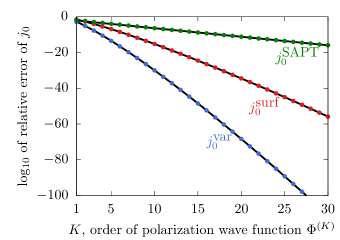
Figure 1: (Color online) Logarithms of errors of $j_{0}$ calculated using the variational, SAPT, and surface-integral formulas. Dots – calculated values, solid lines – the error estimates of Eqs. (14), (32), and (36).

Variational formula. Since $\langle\Phi^{(K)}|\Phi^{(K)}\rangle=1+O(R^{-4})$ and $\langle\Phi^{(K)}|H\Phi^{(K)}\rangle=E_{0}+O(R^{-4})$, the coefficient $j_{0}^{\rm var}[\Phi^{(K)}]$ can be extracted from the expression

$$J_{\rm var}^{*}[\Phi^{(K)}]=\langle\Phi^{(K)}|(H-E_{0}){\cal P}\Phi^{(K)}\rangle.$$ (15)

Writing $\Phi^{(K)}=\varphi^{(0)}F^{(K)}$ one can show that $j_{0}^{\rm var}[\Phi^{(K)}]$ can be obtained from even simpler formula:

$$J_{\rm var}^{**}[\Phi^{(K)}]=\bigg{\langle}{\cal P}\varphi^{(0)}F^{(K)}\bigg{|}\varphi^{(0)}\bigg{(}\frac{\partial}{\partial r_{a}}F^{(K)}+VF^{(K)}\bigg{)}\bigg{\rangle},$$ (16)

in which the Laplacian of $F^{(K)}$ was neglected since it does not contribute to $j_{0}^{\rm var}[\Phi^{(K)}]$.

Approximating $F^{(K)}$ by $\widetilde{F}^{(K)}=\widetilde{f}^{(0)}+\widetilde{f}^{(1)}+\dots+\widetilde{f}^{(K)}$ and noting that $\partial\widetilde{F}^{(k)}/\partial r_{a}+V\widetilde{F}^{(K)}=\widetilde{f}^{(K)}$, cf. Eq. (12), one can represent the asymptotics of $J_{\rm var}^{**}[\Phi^{(K)}]$ in terms of integrals

$$\big{\langle}{\cal P}\varphi^{(0)}\widetilde{f}^{(k_{1})}\big{|}V\varphi^{(0)}\widetilde{f}^{(k_{2})}\big{\rangle}\!=\!-\frac{Re^{-R}}{4k_{1}!k_{2}!}L(k_{1},k_{2})\!\bigg{[}1+O\bigg{(}\!\frac{1}{R}\!\bigg{)}\!\bigg{]}$$ (17)

where

$$L(k_{1},k_{2})=\int_{-1}^{1}d\eta\ (1+\eta)^{2}[\gamma(\eta)]^{k_{1}}[\gamma(-\eta)]^{k_{2}},$$ (18)

and $\gamma(\eta)=(\eta-1)/2+\ln 2-\ln(\eta+1)$. Eqs. (17) and (18) follow from the integration in the elliptic coordinates, $\xi=(r_{a}+r_{b})/R,\eta=(r_{a}-r_{b})/R$, and the integration by parts procedure of Eq. (29) in Ref. Gniewek and Jeziorski (2015).

Using Eqs. (16) and (17) one obtains

$$\frac{2}{e}j_{0}^{\textrm{var}}[\Phi^{(K)}]=-\frac{1}{4K!}\sum_{k=0}^{K}\frac{L(k,K)}{k!}.$$ (19)

For $K=1$ one finds

$$\frac{2}{e}j_{0}^{\textrm{var}}[\Phi^{(1)}]=-\frac{1}{4}\big{[}L(0,1)+L(1,1)\big{]}=-\frac{989}{540}+\frac{\pi^{2}}{9},$$ (20)

in agreement with Ref. Chipman and Hirschfelder (1973). For arbitrary $K$ Eq. (19) can be rewritten as

$$\frac{2}{e}j_{0}^{\textrm{var}}[\Phi^{(K)}]=-\frac{1}{4K!}\bigg{[}M(K)-\sum_{p=1}^{\infty}T^{K}_{p}\bigg{]},$$ (21)

where

$$T_{p}^{K}=L(K+p,K)/(K+p)!,$$ (22)

and

$$M(K)=\sum_{k=0}^{\infty}\frac{L(k,K)}{k!}=\frac{8}{e}\int_{0}^{\infty}x^{K}e^{-x}dx=\frac{8K!}{e}.$$ (23)

To derive Eq. (23) we changed the order of summation and integration, collapsed the exponential series, and used the variable change $x=\gamma(-\eta)$. Since the second-term in the square brackets on the r.h.s. of Eq. (21) vanishes when $K\rightarrow\infty$, cf. Eqs. (31) and (25), we see that $j_{0}^{\textrm{var}}[\Phi^{(K)}]$ converges to the correct value $j_{0}=-1$.

Variational formula — the convergence rate. For large $K$ and $p=1,2$ the integrals $L(K+p,K)$ of Eq. (22) can be approximated using the Laplace’s method Bender and Orszag (1999). To this end we rewrite them as

$$L(K+p,K)=\int_{-1}^{1}(1+\eta)^{2}[\gamma(\eta)]^{p}e^{K\lambda(\eta)}d\eta$$ (24)

where $\lambda(\eta)=\ln\big{[}\gamma(\eta)\gamma(-\eta)\big{]}$. As $\lambda(\eta)$ has a single maximum at $\eta=0$, for large $K$ only $\eta\in[-\epsilon,\epsilon]$ with a small $\epsilon$ contribute significantly to Eq. (24). Approximating $\lambda(\eta)$ for $|\eta|<\epsilon$ by the Taylor expansion, $\lambda(\eta)=\lambda_{0}+\lambda_{2}\eta^{2}+O\big{(}\eta^{3}\big{)}$ converts Eq. (24) into the Gaussian integral, see Ref. Bender and Orszag (1999) for details,

$$L(K+p,K)=\sqrt{\pi/(K|\lambda_{2}|)}\,\,a^{2K+p}\big{[}1+O(K^{-1})\big{]},$$ (25)

where $\lambda_{2}=(4a-1)/(4a^{2})$.

We shall now estimate the contribution of the subsequent $p>2$ terms of the residual series in Eq. (21). The integrals $L(K+p,K)$ can be bounded by the Schwartz inequality

$$L(K+p,K)\leq(P_{2p}Q_{2K})^{1/2},$$ (26)

where, using again Laplace’s method,

$$Q_{m}\equiv\!\!\int_{-1}^{1}\!e^{m\lambda(\eta)}d\eta=\sqrt{\pi/(m|\lambda_{2}|)}\,a^{2m}\bigg{[}1+O\bigg{(}\!\frac{1}{m}\!\bigg{)}\!\bigg{]}$$ (27)

and, using the variable change $t=\ln 2-\ln(t+1)$,

$$P_{m}\equiv\int_{-1}^{1}(1+\eta)^{4}[\gamma(\eta)]^{m}d\eta=32\int_{0}^{\infty}e^{-5t}\big{[}e^{-t}+t-1\big{]}^{m}dt.$$ (28)

Since $e^{-t}+t-1\leq t$ for $t\geq 0$, it follows that $P(m)\leq(32/5)m!/5^{m}$, so that $T^{K}_{p}\leq\widetilde{T}^{K}_{p}$, where

$$\widetilde{T}^{K}_{p}=4\big{[}\tfrac{2}{5}(2p)!Q_{2K}\big{]}^{1/2}\,5^{-p}/(K+p)!.$$ (29)

Since $\widetilde{T}^{K}_{p+1}/\widetilde{T}^{K}_{p}\leq 2/5$, we can estimate the contributions of the terms with $p\geq 3$ by

$$\frac{1}{T^{K}_{1}}\sum_{p=3}^{\infty}T^{K}_{p}\leq\frac{5}{3}\frac{\widetilde{T}^{K}_{3}}{T^{K}_{1}}=\frac{D\,K^{1/4}}{(K+2)(K+3)}\bigg{[}1+O(K^{-1})\bigg{]},$$ (30)

where $D=16[(1-4a)/(2\pi)]^{1/4}/(25a^{3/2})$. In view of Eq. (25), $T_{2}^{K}\sim a^{2K+2}/(K+2)!$, so that finally

$$\sum_{p=1}^{\infty}T^{K}_{p}=T^{K}_{1}\big{[}1+O\big{(}K^{-1}\big{)}\big{]}.$$ (31)

Thus, the error of $j_{0}^{\rm var}[\Phi^{(K)}]$ is dominated by the $p=1$ term in the sum in Eq. (21),

$$j_{0}-j_{0}^{\rm var}[\Phi^{(K)}]=-\frac{A\ a^{2K+2}}{\sqrt{K}K!(K+1)!}\bigg{[}1+O\big{(}K^{-1}\big{)}\bigg{]},$$ (32)

where $A=e\sqrt{\pi}/(4\sqrt{1-4a})$. The rapid fall-off of the error of $j_{0}^{\rm var}[\Phi^{(K)}]$ can be seen in Fig. 1.

SAPT formula. To obtain $j_{0}^{\textrm{SAPT}}[\Phi^{(K)}]$ it is sufficient to consider the following approximation to $J_{\textrm{SAPT}}[\Phi^{(K)}]$,

$$J_{\textrm{SAPT}}^{*}[\Phi^{(K)}]=\langle\varphi^{(0)}|V{\cal P}\varphi^{(0)}F^{(K)}\rangle.$$ (33)

Approximating $F^{(K)}$ by the sum of functions $\widetilde{f}^{(k)}(r_{a})$ one can represent $j_{0}^{\rm var}[\Phi^{(K)}]$ in terms of integrals $\langle\varphi^{(0)}|V{\cal P}\varphi^{(0)}\widetilde{f}^{(k)}(r_{a})\rangle$. Using Eq. (17) one obtains

$$\frac{2}{e}j_{0}^{\textrm{SAPT}}[\Phi^{(K)}]=-\frac{1}{4}\sum_{k=0}^{K}\frac{L(k)}{k!},$$ (34)

with $L(k)=L(k,0)$. When $K\rightarrow\infty$, the sum on the r.h.s. is equal to $M(0)$, so in view of Eq. (23), $j_{0}^{\textrm{SAPT}}[\Phi^{(K)}]$ converges to the correct value $j_{0}=-1$.

To calculate the error of $j_{0}^{\textrm{SAPT }}[\Phi^{(K)}]$ we need the integrals $L(k)$, for which the variable change $t=\ln 2-\ln(t+1)$ gives

$$L(k)=8\!\!\int_{0}^{\infty}\!\!\!e^{-3t}\big{[}e^{-t}+t-1\big{]}^{k}dt=\sum_{l=0}^{k}\frac{8k!e_{k-l}(-l-3)}{l!(l+3)^{k-l+1}},$$ (35)

where $e_{n}(x)$ is the exponential sum function, i.e. the series of $e^{x}$ truncated after the $x^{n}/n!$ term. The large-$k$ asymptotics of $L(k)$ is given by the first, $l=0$ term in the sum in Eq. (35). It follows that

$$j_{0}-j_{0}^{\textrm{SAPT}}[\Phi^{(K)}]=-\frac{1}{6e^{2}}\,3^{-K}+O(4^{-K}).$$ (36)

The error of $j_{0}^{\textrm{SAPT}}[\Phi^{(K)}]$ can be compared to the errors of the other two formulas in Fig. 1.

Summary and conclusions. By solving analytically the model system of the hydrogen atom interacting with a proton we found that all three exchange energy formulas considered by us correctly predict the large-$R$ behavior of the exchange energy if the primitive function is approximated by the standard polarization expansion. The correct limit is however approached with very different convergence rates. In the case of the SAPT formula, the convergence is geometric with the error decaying as $1/3^{K}$, where K is the order of the applied polarization theory. The convergence of the surface-integral formula is exponential, with the error decreasing as $a^{K}/(K+1)!$, where $a=\ln 2-1/2$. The best convergence occurs for the variational formula, for which the error falls off as $K^{1/2}[a^{K}/(K+1)!]^{2}$. The observed convergence rates are significantly faster than those resulting from approximating the primitive function through the multipole expansion Gniewek and Jeziorski (2015, 2016). To make a meaningful comparison, cf. Table 1, we note that $\Phi^{(K)}$ and the sum of the mulitpole expansion through the 2$K$th order in $1/R$, denoted by $\Phi_{2K}$, are both accurate through the (2$K$)th order in $1/R$. However, $\Phi^{(K)}$, unlike $\Phi_{2K}$, includes a selective infinite order summation of higher $R^{-k}$, $k>2K$ terms. The inspection of Table 1 shows that this infinite order, selective summation is very effective in computing the exchange energy, independently of the exchange energy expression employed.

The main conclusion of our investigation is that the exchange energy, an electron tunneling effect, can be determined from the knowledge of the wave function which reflects only the polarization mechanism of interatomic interaction. We have shown that this determination is particularly effective when the variational principle is employed in the perturbation treatment of molecular interactions. We expect that this conclusion is general and applies also to interactions of larger systems.

Table 1: Decay rate of the error of the leading term of exchange energy calculated using truncated multipole $\Phi_{2K}$ (Ref. Gniewek and Jeziorski (2016)) and polarization $\Phi^{(K)}$ series. $a=\ln 2-\frac{1}{2}\approx 1/5$.

	$\Phi=\Phi_{2K}$	$\Phi=\Phi^{(K)}$
$j_{0}^{\textrm{surf}}[\Phi]$	$\displaystyle\frac{1}{4^{K}}$	$\displaystyle\frac{a^{K}}{(K+1)!}$
$j_{0}^{\textrm{SAPT}}[\Phi]$	$\displaystyle\frac{1}{K^{2}}$	$\displaystyle\frac{1}{3^{K}}$
$j_{0}^{\textrm{var}}[\Phi]$	$\displaystyle\frac{1}{16^{K}}$	$\displaystyle\frac{a^{2K}}{K!(K+1)!\sqrt{K}}$