Points on manifolds with asymptotically optimal covering radius

Abstract.

Given a finite set of points on the Euclidean sphere, the worst case quadrature error in Sobolev spaces has recently been shown to provide upper bounds on the covering radius of the point set. Moreover, quasi-Monte Carlo integration points on the sphere achieve the asymptotically optimal covering radius. Here, we extend these results to points on compact smooth Riemannian manifolds and provide numerical experiments illustrating our findings for the Grassmannian manifold.

1. Introduction

Many discretization schemes in numerical analysis are based on finite samples that cover the underlying space sufficiently well, i.e., the sampling points have small covering radius. One way of measuring the covering’s efficiency is by its cardinality in comparison to its covering radius.

Quasi-Monte Carlo integration points have been investigated in [7] for compact smooth Riemannian manifolds. In the special case of the Euclidean sphere, it is shown recently in [9] that the worst case error of integration bounds the covering radius and that thereby quasi-Monte Carlo integration points provide asymptotically optimal covering radii.

Here, we extend these results from the sphere to compact smooth Riemannian manifolds. These theoretical results are derived by combining the ideas in [7] with those in [9].

In the second part of the present note, we numerically construct a sequence of quasi-Monte Carlo integration points for the Grassmannian manifold and illustrate numerically that their covering radii indeed behave in accordance to the theoretical findings, hence, asymptotically optimal.

Our quasi-Monte Carlo integration points are cubatures (in fact designs) in Grassmannians that have been studied in [2, 3, 4, 5] from a theoretical point of view, see [18] for the construction through numerical minimization. For related results on cubatures in more classical settings, see [17, 23, 24, 26, 28, 31, 32] and, for further related results, we refer to [10, 13, 14, 19, 20, 22, 27] and references therein.

The outline is as follows. In Section 2, we briefly discuss the concept of asymptotically optimal covering radii. Low-cardinality cubature points are introduced in Section 3, where we also state our main theoretical result. In Section 4 we state the bound on the covering radius by the worst case error of integration. Section 5 is dedicated to the proof of this bound. In Section 6, we illustrate our theoretical findings by numerical experiments for the Grassmannian manifold $\mathcal{G}_{2,4}$.

2. Optimal asymptotics of the covering radius

Let $\mathcal{M}$ be a compact smooth $d$-dimensional Riemannian manifold. We denote its normalized Riemannian measure by $\mu$ and its Riemannian distance by $\operatorname{dist}$. Given any finite collection of points $\{x_{j}\}_{j=1}^{n}\subset\mathcal{M}$, the covering radius $\rho$ is

$$\rho:=\rho(\{x_{j}\}_{j=1}^{n}):=\sup_{x\in\mathcal{M}}\min_{1\leq j\leq n}\operatorname{dist}(x,x_{j}).$$

For $B_{r}(x):=\{y\in\mathcal{M}:\operatorname{dist}(x,y)\leq r\}$ denoting the ball of radius $r$ centered at $x\in\mathcal{M}$, the union $\bigcup_{j=1}^{n}B_{\rho}(x_{j})$ covers $\mathcal{M}$ completely. By compactness of $\mathcal{M}$ we have

(1) $$\mu(B_{r}(x))\asymp r^{d},\quad x\in\mathcal{M},\quad 0<r\leq 1,$$

where the constants do not depend on $x$ or $r$. Hence, the line of inequalities $\mu(\mathcal{M})\leq\sum_{j=1}^{n}\mu(B_{\rho}(x_{j}))\lesssim n\rho^{d}$ leads to the lower bound

(2) $$n^{-\frac{1}{d}}\lesssim\rho.$$

Definition 2.1.

Given a sequence of $n_{i}$ points $\{x^{i}_{j}\}_{j=1}^{n_{i}}\subset\mathcal{M}$, $i=1,2,\ldots$, with $n_{i}\rightarrow\infty$, we say that the corresponding sequence of covering radii $\rho_{i}$ is asymptotically optimal if the lower bound (2) is matched, i.e., if $\rho_{i}\asymp n_{i}^{-\frac{1}{d}}.$

According to [29], the expectation of the covering radius $\rho$ of $n$ random points $\{x_{j}\}_{j=1}^{n}$, independently identically distributed according to $\mu$, satisfies

(3) $$\mathbb{E}\rho\asymp n^{-\frac{1}{d}}\log(n)^{\frac{1}{d}}.$$

Hence, there is an additional logarithmic factor, so that random points do not provide optimal covering radii.

In this brief note, we shall verify that the recently introduced concept of quasi-Monte Carlo systems, cf. [7, 8], lead to point sets with asymptotically optimal covering radii. This generalizes results for the sphere in [9] to compact smooth Riemannian manifolds.

3. Optimal coverings from low-cardinality cubatures

Let $\{\varphi_{\ell}\}_{\ell=0}^{\infty}$ be the collection of orthonormal eigenfunctions of the Laplace-Beltrami operator $\Delta$ on $\mathcal{M}$ with eigenvalues $\{-\lambda_{\ell}\}_{\ell=0}^{\infty}$ arranged by $0=\lambda_{0}\leq\lambda_{1}\leq\ldots$. We denote by $L_{p}(\mathcal{M})$, $1\leq p<\infty$, the Banach space of complex-valued $\mu$-measurable functions on $\mathcal{M}$, whose $p$-th power of the absolute value is integrable (with the standard modifications when $p=\infty$).

The space of diffusion polynomials of bandwidth $t\geq 0$ is

(4) $$\Pi_{t}:=\operatorname*{span}\{\varphi_{\ell}:\lambda_{\ell}\leq t^{2}\}.$$

For $\{x_{j}\}_{j=1}^{n}\subset\mathcal{M}$ and weights $\{\omega_{j}\}_{j=1}^{n}\subset\mathbb{R}$, we say that $\{(x_{j},\omega_{j})\}_{j=1}^{n}$ is a cubature for $\Pi_{t}$ if

(5) $$\int_{\mathcal{M}}f(x)d\mu(x)=\sum_{j=1}^{n}\omega_{j}f(x_{j}),\quad\text{for all }f\in\Pi_{t}.$$

The number $t$ refers to the strength of the cubature.

Weyl’s estimates on the spectrum of an elliptic operator yield

$$\dim(\Pi_{t})\asymp t^{d},$$

cf. [25, Theorem 17.5.3]. Therefore, any sequence of cubatures $\{(x^{i}_{j},\omega^{i}_{j})\}_{j=1}^{n_{i}}$ of strength $t_{i}$ must obey $n_{i}\gtrsim t_{i}^{d}$.

Definition 3.1.

We call a sequence of cubatures $\{(x^{i}_{j},\omega^{i}_{j})\}_{j=1}^{n_{i}}$ for $\Pi_{t_{i}}$ satisfying

(6) $$n_{i}\asymp t_{i}^{d}$$

with $n_{i}\rightarrow\infty$ a low-cardinality cubature sequence.

The above definition makes sense since there do exist sequences of cubatures $\{(x^{i}_{j},\omega^{i}_{j})\}_{j=1}^{n_{i}}$ of strength $t_{i}$ with positive weights and $n_{i}\rightarrow\infty$ satisfying (6), cf. [16]. We now state our main theoretical result.

Theorem 3.2.

The covering radius of any low-cardinality cubature sequence with positive weights is asymptotically optimal.

The remaining part of the present paper is dedicated to prove Theorem 3.2 and to numerically illustrate our findings on the Grassmannian manifold. We conclude this section with a remark concerning the weights.

Remark 3.3.

Cubatures of strength $t$, whose weights are all the same, $\omega_{j}=\frac{1}{n}$, for $j=1,\ldots,n$, are also called $t$-designs. If $\mathcal{M}=\mathbb{S}^{d}\subset\mathbb{R}^{d+1}$ is the unit Euclidean sphere, then there are $t$-designs satisfying (6), cf. [6]. By identifying $x\in\mathbb{S}^{d}$ with $-x$, the analogous statement holds for the projective space. For general $\mathcal{M}$, however, we only know that $t$-designs exist, cf. [30], but it is still an open problem whether or not the asymptotics (6) can be achieved.

4. Worst case error of integration

To prove Theorem 3.2, we follow the approach for the sphere in [9]. We shall first introduce the worst case error of integration and shall check that it provides an upper bound on the covering radius. Next, we shall consider the concept of quasi-Monte Carlo points, i.e., points whose worst case error of integration decays sufficiently fast, so that the covering radius is asymptotically optimal. Finally, we shall recapitulate from [7] that low-cardinality cubature points with positive weights are indeed quasi-Monte Carlo points.

The worst case error of integration of points $\{x_{j}\}_{j=1}^{n}\subset\mathcal{M}$ and weights $\{\omega_{j}\}_{j=1}^{n}\subset\mathbb{R}$ with respect to some Banach space $\mathcal{H}$ of complex-valued functions on $\mathcal{M}$ is

(7) $$\operatorname{wce}(\{(x_{j},\omega_{j})\}_{j=1}^{n},\mathcal{H}):=\sup_{\begin{subarray}{c}f\in\mathcal{H}\\ \|f\|_{\mathcal{H}}\leq 1\end{subarray}}\Big{|}\int_{\mathcal{M}}f(x)d\mu(x)-\sum_{j=1}^{n}\omega_{j}f(x_{j})\Big{|}.$$

Although suppressed by our notation, (7) depends on the particular norm $\|\cdot\|_{\mathcal{H}}$, which shall always be clear from the context in the present manuscript. For most parts, we take $\mathcal{H}$ to be a Sobolev space, which we define next. The Fourier transform of $f\in L_{p}(\mathcal{M})$ with $1\leq p\leq\infty$ is

$$\hat{f}(\ell):=\int_{\mathcal{M}}f(x)\overline{\varphi_{\ell}(x)}d\mu(x),\qquad\ell=0,1,2,\ldots,$$

and extends to distributions on $\mathcal{M}$. The Sobolev space $W^{s}_{p}(\mathcal{M})$, for $1\leq p\leq\infty$ and $s>0$, is the set of all distributions on $\mathcal{M}$ with $(I+\Delta)^{s/2}f\in L_{p}(\mathcal{M})$, i.e., with

(8) $$\|f\|_{W^{s}_{p}}:=\|(I+\Delta)^{s/2}f\|_{L_{p}}=\|\sum_{\ell=0}^{\infty}(1+\lambda_{\ell})^{s/2}\hat{f}(\ell)\varphi_{\ell}\|_{L_{p}}<\infty.$$

Note that $W^{s}_{p}(\mathcal{M})$ is contained in the space of continuous functions on $\mathcal{M}$ provided that $s>d/p$, cf. [7]. We shall stick to this range throughout the present paper.

It turns out that the covering radius is bounded by the worst case error. The following result has been derived in [9] for $\mathcal{M}$ being the Euclidean sphere and constant weights $\omega_{j}^{i}=1/n_{i}$.

Proposition 4.1.

Let $1\leq p\leq\infty$ and $s>d/p$ be given. Then for any points $\{x_{j}\}_{j=1}^{n}\subset\mathcal{M}$ and weights $\{\omega_{j}\}_{j=1}^{n}\subset\mathbb{R}$ with covering radius $\rho$ it holds

(9) $$\rho\lesssim\big{[}\operatorname{wce}(\{(x_{j},\omega_{j})\}_{j=1}^{n},W^{s}_{p}(\mathcal{M}))\big{]}^{1/(s+d/q)},$$

where $1/p+1/q=1$. The constants may only depend on $\mathcal{M}$, $s$, and $p$.

We shall postpone the proof of Proposition 4.1 to Section 5. At this point we turn to sequences of points whose worst case error of integration satisfies decay conditions, which connects to the covering radius via the bound (9). The following definition is due to [7, 8].

Definition 4.2.

Given $1\leq p\leq\infty$ and $s>d/p$, a sequence $\{(x^{i}_{j},\omega^{i}_{j})\}_{j=1}^{n_{i}}$, $i=1,2,\ldots$, of points $\{x_{j}^{i}\}_{j=1}^{n_{i}}\subset\mathcal{M}$ and weights $\{\omega_{j}^{i}\}_{j=1}^{n_{i}}\subset\mathbb{R}$ with $n_{i}\rightarrow\infty$ is called a quasi-Monte Carlo (qMC) system for $W^{s}_{p}(\mathcal{M})$ if

(10) $$\operatorname{wce}(\{(x^{i}_{j},\omega^{i}_{j})\}_{j=1}^{n_{i}},W^{s}_{p}(\mathcal{M}))\lesssim n_{i}^{-\frac{s}{d}}.$$

According to [7], low-cardinality cubature sequences with positive weights are qMC systems:

Proposition 4.3 ([7]).

For $1\leq p\leq\infty$ and $s>d/p$, any low-cardinality cubature sequence $\{(x^{i}_{j},\omega^{i}_{j})\}_{j=1}^{n_{i}}$ with positive weights is a qMC system for $W^{s}_{p}(\mathcal{M})$.

For $1\leq p\leq p^{\prime}\leq\infty$, due to (8), the space $W^{s}_{p^{\prime}}(\mathcal{M})$ is continuously embedded into $W^{s}_{p}(\mathcal{M})$ with $\|f\|_{W^{s}_{p^{\prime}}}\leq\|f\|_{W^{s}_{p}}$, for $f\in W^{s}_{p^{\prime}}(\mathcal{M})$. Thus, if $s>d/p$ and $\{(x^{i}_{j},\omega^{i}_{j})\}_{j=1}^{n_{i}}$ is a qMC system for $W^{s}_{p}(\mathcal{M})$, then it is also a sequence of qMC systems for $W^{s}_{p^{\prime}}(\mathcal{M})$. If $\mathcal{M}$ is the sphere, then the latter becomes [9, Theorem 4.2]. Therefore, $p=1$ is the strongest requirement among the qMC properties.

Remark 4.4.

If $\{(x^{i}_{j},\omega^{i}_{j})\}_{j=1}^{n_{i}}$ is a qMC system for some $p\geq 1$, then Proposition 4.1 yields that its covering radii are bounded by

$$\rho_{i}\lesssim n_{i}^{-\frac{1}{d}(\frac{s}{s+d(1-1/p)})}.$$

Thus, qMC systems for $p=1$ provide

$$\rho_{i}\lesssim\big{[}\operatorname{wce}(\{(x^{i}_{j},\omega^{i}_{j})\}_{j=1}^{n_{i}},W^{s}_{1}(\mathcal{M}))\big{]}^{1/s}\lesssim n_{i}^{-\frac{1}{d}},$$

so that Theorem 3.2 is a consequence of Propositions 4.1 and 4.3. Hence, to complete the proof of Theorem 3.2, it only remains to verify Proposition 4.1, which is the topic of the subsequent section.

Before we proceed to the proof of Proposition 4.1, we shall discuss a method to compute the worst case error of integration in $W^{s}_{2}(\mathcal{M})$, the latter being a Hilbert space with inner product

(11) $$\langle f,g\rangle_{W^{s}_{2}}=\sum_{\ell=0}^{\infty}(1+\lambda_{\ell})^{s}\hat{f}(\ell)\overline{\hat{g}(\ell)},\quad f,g\in W^{s}_{2}(\mathcal{M}).$$

The Bessel kernel $K^{s}_{B}:\mathcal{M}\times\mathcal{M}\rightarrow\mathbb{R}$ given by

(12) $$K^{s}_{B}(x,y)=\sum_{\ell=0}^{\infty}(1+\lambda_{\ell})^{-s}\varphi_{\ell}(x)\overline{\varphi_{\ell}(y)}$$

is the reproducing kernel for $W^{s}_{2}(\mathcal{M})$ with respect to the inner product (11) provided that $s>d/2$. For later reference we consider a slightly more abstract setting. If $K:\mathcal{M}\times\mathcal{M}\rightarrow\mathbb{R}$ is a reproducing kernel for some reproducing kernel Hilbert space $H_{K}$ of continuous functions on $\mathcal{M}$, then the worst case error of integration is

(13) $$\operatorname{wce}(\{(x_{j},\omega_{j})\}_{j=1}^{n},H_{K})^{2} =\sum_{j,j^{\prime}=1}^{n}\omega_{j}\omega_{j^{\prime}}K(x_{j},x_{j^{\prime}})-2\sum_{j=1}^{n}\omega_{j}\int_{\mathcal{M}}K(x_{j},x)d\mu(x)$$

$$\qquad+\int_{\mathcal{M}}\int_{\mathcal{M}}K(x,y)d\mu(x)d\mu(y),$$

cf. [21, Theorem 2.7], see also [28]. Note, the norm in $H_{K}$ is uniquely determined by its reproducing kernel $K$. If $K$ has the Fourier expansion

(14) $$K(x,y)=\sum_{\ell=0}^{\infty}\hat{K}(\ell)\varphi_{\ell}(x)\overline{\varphi_{\ell}(y)}$$

with $\hat{K}(\ell)\in\mathbb{C}$, for $\ell=0,1,\ldots$, then (13) becomes

(15) $$\operatorname{wce}(\{(x_{j},\omega_{j})\}_{j=1}^{n},H_{K})^{2}=\sum_{j,j^{\prime}=1}^{n}\omega_{j}\omega_{j^{\prime}}K(x_{j},x_{j^{\prime}})+\hat{K}(0)(1-2\sum_{j=1}^{n}\omega_{j}),$$

where we assume without loss of generality $\varphi_{0}\equiv 1$. For the Bessel kernel $K^{s}_{B}$, we observe $\hat{K}^{s}_{B}(\ell)=(1+\lambda_{\ell})^{-s}$ with $\hat{K}^{s}_{B}(0)=1$

We conclude this section by the following result on the worst case error of uniformly distributed random points, for which constant weights $\omega_{j}=1/n$ are the natural choice.

Proposition 4.5.

If $K$ is a reproducing kernel on $\mathcal{M}$ and $x_{1},\ldots,x_{n}$ are random points on $\mathcal{M}$, independently identically distributed according to $\mu$, then it holds

$$\sqrt{\mathbb{E}\Big{[}\operatorname{wce}(\{(x_{j},\frac{1}{n})\}_{j=1}^{n},H_{K})^{2}\Big{]}}=cn^{-\frac{1}{2}},$$

where

(16) $$c^{2}=\int_{\mathcal{M}}K(x,x)d\mu(x)-\int_{\mathcal{M}}\int_{\mathcal{M}}K(x,y)d\mu(x)d\mu(y).$$

By applying (14), the constant (16) is $c^{2}=\sum_{\ell=1}^{\infty}\hat{K}(\ell)$. For the Bessel kernel $K^{s}_{B}$, the condition $s>d/2$ implies that $\frac{s}{d}>\frac{1}{2}$, so that on average qMC systems indeed perform better than random points for smooth functions. The proof of Proposition 4.5 follows from the lines in [8] when replacing the sphere by $\mathcal{M}$. In fact, Proposition 4.5 is already contained in [21, Corollary 2.8], see also [28].

5. Proof of Proposition 4.1

The proof of Proposition 4.1 relies on findings in [7]. We recapitulate the following localization result, which is one of the key ingredients for the proof of Proposition 4.1.

Lemma 5.1.

For $s\in\mathbb{R}$ and $h:\mathbb{R}\rightarrow\mathbb{R}$ being a smooth function, supported in the interval $[\frac{1}{2},2]$, the kernel

$$K^{s}_{r}(x,y):=\sum_{\ell=0}^{\infty}h(\frac{\lambda_{\ell}}{r})(1+\lambda_{\ell})^{-s/2}\varphi_{\ell}(x)\overline{\varphi_{\ell}(y)}$$

is bounded by

(17) $$\big{\|}\int_{\mathcal{M}}|K^{s}_{r}(\cdot,y)|d\mu(y)\big{\|}_{L_{\infty}}\lesssim r^{-s},\qquad r>0,$$

where the constant does not depend on $r$.

Proof.

According to [7, Lemma 2.8], the estimate

$$|K^{s}_{r}(x,y)|\lesssim r^{d-s}(1+r\operatorname{dist}(x,y))^{-(d+1)},\quad r>0,$$

holds and leads to the requested assertion

$$\sup_{x\in\mathcal{M}}\big{|}\int_{\mathcal{M}}|K^{s}_{r}(x,y)|d\mu(y)\big{|} \lesssim r^{d-s}\sup_{x\in\mathcal{M}}\int_{\mathcal{M}}(1+r\operatorname{dist}(x,y))^{-(d+1)}d\mu(y)$$

$$\lesssim r^{-s}\sup_{x\in\mathcal{M}}\int_{\mathcal{M}}r^{d}(1+r\operatorname{dist}(x,y))^{-(d+1)}d\mu(y)$$

$$\lesssim r^{-s}.\qed$$

We shall make use of Lemma 5.1 to verify the following result.

Lemma 5.2.

Let $R,s>0$, and $1\leq p\leq\infty$ be fixed. For any $0<r\leq R$ and $z\in\mathcal{M}$, there is a function $f:=f_{r,z}\in\mathcal{C}^{\infty}(\mathcal{M})$ with support in $B_{r}(z)$, such that

(18) $$\|f\|_{W^{s}_{p}}\lesssim r^{-s+d/p},\qquad r^{d}\lesssim\int_{\mathcal{M}}f(x)d\mu(x),$$

where the constants do not depend on $z$ or $r$.

Proof.

As in [7, Proof of Theorem 2.16], for any radius $0<r\leq R$ and $z\in\mathcal{M}$, there is a function $f:=f_{r,z}\in\mathcal{C}^{\infty}(\mathcal{M})$ with support in $B_{r}(z)$, such that, for $\ell=0,1,2,\ldots$,

(19) $$\|\Delta^{\ell}f\|_{L_{\infty}}\lesssim r^{-2\ell},\qquad r^{d}\lesssim\int_{\mathcal{M}}f(x)d\mu(x),$$

where by compactness of $\mathcal{M}$ the constants do not depend on $z$ or $r$.

Similarly as in [7, Proof of Theorem 2.16], we bound the norm $\|f\|_{W_{p}^{s}}=\|(I+\Delta)^{s}f\|_{L_{p}}$ by using a dyadic decomposition of unity of the Fourier domain, see, for instance, [32]. That is, we set $h(x):=g(x)-g(2x)$ for some smooth function $g:\mathbb{R}\to\mathbb{R}$ satisfying

$$g(x)=\begin{cases}1,&x\leq 1,\\ 0,&x\geq 2,\end{cases}$$

and obtain $\operatorname{supp}(h)\subset[1/2,2]$ with

$$\sum_{m=-\infty}^{\infty}h(2^{-m}x)=\begin{cases}1,&x>0,\\ 0,&\text{else}.\end{cases}$$

Using the Fourier expansion $f=\sum_{\ell=0}^{\infty}\hat{f}(\ell)\varphi_{\ell}$ we arrive at

$$(I+\Delta)^{s/2}f=\hat{f}(0)+\sum_{\ell=0}^{\infty}\;\sum_{m=-\infty}^{\infty}h(2^{-m}\lambda_{\ell})(1+\lambda_{\ell})^{s/2}\hat{f}(\ell)\varphi_{\ell}.$$

Fixing an integer $L>s/2$ and applying the notation of Lemma 5.1 with $\hat{f}(\ell)=\int_{\mathcal{M}}f(y)\overline{\varphi_{\ell}(y)}d\mu(y)$ lead to

$$(I+\Delta)^{s/2}f =\hat{f}(0)+\sum_{2^{m}\leq 1/r}\int_{\mathcal{M}}K^{-s}_{2^{m}}(\cdot,y)f(y)d\mu(y).$$

$$\qquad\quad+\sum_{2^{m}>1/r}\int_{\mathcal{M}}K^{2L-s}_{2^{m}}(\cdot,y)(I+\Delta)^{L}f(y)d\mu(y).$$

We shall now bound the three terms of the right hand side separately. First, the Hölder inequality with (19) for $\ell=0$ yields

$$|\hat{f}(0)|=\big{|}\int_{\mathcal{M}}f(y)d\mu(y)\big{|}\leq\|f\|_{L_{\infty}}\mu(\mathcal{M})\lesssim 1\lesssim r^{-s},$$

where the last estimate is due to $r$ being bounded from above and $s>0$. To bound the second term, we apply Lemma 5.1 and derive

$$\|\sum_{2^{m}\leq 1/r}\int_{\mathcal{M}}K^{-s}_{2^{m}}(\cdot,y)f(y)d\mu(y)\|_{L_{\infty}} \leq\sum_{2^{m}\leq 1/r}\|\int_{\mathcal{M}}|K^{-s}_{2^{m}}(\cdot,y)|d\mu(y)\|_{L_{\infty}}\|f\|_{L_{\infty}}$$

$$\lesssim\sum_{2^{m}\leq 1/r}\|\int_{\mathcal{M}}|K^{-s}_{2^{m}}(\cdot,y)|d\mu(y)\|_{L_{\infty}}$$

$$\lesssim\sum_{2^{m}\leq 1/r}2^{ms}\lesssim r^{-s}.$$

Lemma 5.1 also leads to a bound on the third term by

$$\|\sum_{2^{m}>1/r}\int_{\mathcal{M}}K^{2L-s}_{2^{m}}(\cdot,y)(I+\Delta)^{L}f(y)d\mu(y)\|_{L_{\infty}}$$

$$\lesssim\sum_{2^{m}>1/r}\|\int_{\mathcal{M}}K^{2L-s}_{2^{m}}(\cdot,y)(I+\Delta)^{L}f(y)d\mu(y)\|_{L_{\infty}}$$

$$\lesssim\sum_{2^{m}>1/r}\|\int_{\mathcal{M}}K^{2L-s}_{2^{m}}(\cdot,y)d\mu(y)\|_{L_{\infty}}\|(I+\Delta)^{L}f\|_{L_{\infty}}$$

$$\lesssim\sum_{2^{m}>1/r}2^{-(2L-s)m}r^{-2L}$$

$$\lesssim r^{2L-s}r^{-2L}=r^{-s},$$

where we have also applied (19) and $r$ being bounded from above.

Thus, we obtain

(20) $$\|(I+\Delta)^{s/2}f\|_{L_{\infty}}\lesssim r^{-s},$$

where the constants do not depend on $z$ or $r$ To cover the range $1\leq p<\infty$, we recall that $f$ is supported on $B_{r}(z)$, so that the Hölder inequality with (1) yields

(21) $$\|(I+\Delta)^{s/2}f\|^{p}_{L_{p}}\lesssim r^{-ps}\mu(B_{r}(z))\lesssim r^{-sp+d},$$

which concludes the proof. ∎

We are now prepared to complete the proof of our main theoretical result.

Proof of Proposition 4.1.

For a given point set $\{x_{j}\}_{j=1}^{n}\subset\mathcal{M}$ with covering radius $\rho$, let $z$ be a center of a maximal hole, i.e.,

(22) $$\mathring{B}_{\rho}(z)\cap\{x_{j}\}_{j=1}^{n}=\emptyset,$$

where $\mathring{B}_{\rho}(z)=\{x\in\mathcal{M}:\operatorname{dist}(x,z)<\rho\}$ denotes the interior of $B_{\rho}(z)$. Note that $\rho$ is bounded by the diameter of $\mathcal{M}$. Let $f=f_{\rho,z}\in\mathcal{C}^{\infty}(\mathcal{M})$ be as in Lemma 5.2, i.e., $\operatorname{supp}(f)\subset B_{\rho}(z)$ and (18) holds with $r=\rho$. Since $f$ must vanish outside of $\mathring{B}_{\rho}(z)$, (22) implies $f(x_{j})=0$, for all $j=1,\ldots,n$. Thus, the definition of the worst case error of integration yields

$$\operatorname{wce}(\{(x_{j},\omega_{j})\}_{j=1}^{n},W^{s}_{p}(\mathcal{M})) \geq\frac{\big{|}\int_{\mathcal{M}}f(x)d\mu(x)-0\big{|}}{\|f\|_{W^{s}_{p}}}\gtrsim\frac{\rho^{d}}{\rho^{-s+d/p}}=\rho^{s+d/q},$$

with $1/p+1/q=1$, and the constant does not depend on $z$ or $\rho$. ∎

6. Numerical experiments for the Grassmannian manifold

This section is dedicated to illustrate the results of the previous sections for the special case of the Grassmannian manifold, i.e., the collection of $k$-dimensional linear subspaces in $\mathbb{R}^{m}$, which we identify with the set of orthogonal projectors on $\mathbb{R}^{m}$ of rank $k$, denoted by

(23) $$\operatorname{\mathcal{G}}_{k,m}:=\{P\in\mathbb{R}^{m\times m}:P^{\top}=P,\;P^{2}=P,\;\operatorname{\operatorname{trace}}(P)=k\}.$$

Hence, the Grassmannian $\mathcal{G}_{k,m}$ can be considered as a $k(m-k)$-dimensional submanifold of the Euclidean space $\mathbb{R}^{m^{2}}\cong\mathbb{R}^{m\times m}$. Moreover the Euclidean space $\mathbb{R}^{m^{2}}$ induces a Riemannian metric, which in turn yields the canonical probability measure and the canonical geodesic distance on the Grassmannian $\mathcal{G}_{k,m}$ denoted by $\mu_{k,m}$ and $\operatorname{dist}_{k,m}$, respectively. In particular, the geodesic distance $\operatorname{dist}_{k,m}(P,Q)$ between $P,Q\in\operatorname{\mathcal{G}}_{k,m}$ is proportional to the $2$-norm of the corresponding principal angles $\theta_{1},\ldots\theta_{k}$ between the subspace associated to $P$ and $Q$. More precisely, it can be computed by

(24) $$\operatorname{dist}_{k,m}(P,Q)=\sqrt{2}\sqrt{\theta^{2}_{1}+\ldots+\theta^{2}_{k}},$$

where $\theta_{i}=\arccos(\sqrt{y_{i}})$ and $y_{1},\ldots,y_{k}$ are the $k$-largest eigenvalues of $PQ$ (counted with multiplicities). Note that the factor of $\sqrt{2}$ accounts for the particular embedding (23) since then

(25) $$\operatorname{dist}_{k,m}(P,Q)=\|P-Q\|_{\mathrm{F}}+o(\|P-Q\|_{\mathrm{F}}^{2}),\qquad P,Q\in\mathcal{G}_{k,m},$$

where $\|X\|_{\mathrm{F}}$ is the Frobenius-norm of $X\in\mathbb{R}^{m\times m}$.

6.1. Cubature points

Theorem 3.2 tells us that low-cardinality cubature points with positive weights inherit asymptotically optimal covering radii. To illustrate this result, we first construct a sequence of cubature points. It is known that any collection of points $\{P_{j}\}_{j=1}^{n}\subset\mathcal{G}_{k,m}$ satisfies

(26) $$\frac{1}{n^{2}}\sum_{j,j^{\prime}=1}^{n}\operatorname{\operatorname{trace}}(P_{j},P_{j^{\prime}})^{i}\geq\int_{\operatorname{\mathcal{G}}_{k,m}}\int_{\operatorname{\mathcal{G}}_{k,m}}\operatorname{\operatorname{trace}}(P,Q)^{i}d\mu_{k,m}(P)d\mu_{k,m}(Q),$$

for $i=1,2,\ldots$, cf. [5]. According to [11], equality in (26) yields a design of strength $t_{i}=i\frac{2}{\sqrt{k}}$, see also [18]. Hence, (26) provides us with a simple approach to numerically compute cubature points by minimization and checking for equality.

Our numerical experiments shall focus on $\mathcal{G}_{2,4}$, which has dimension $d=4$, so that for low-cardinality cubature sequences the number of cubature points must satisfy $n_{i}\asymp i^{4}\asymp{t_{i}}^{4}$. Indeed, we have chosen

$$n_{i}=\Big{\lfloor}\tfrac{1}{3}(i+1)^{2}(1+i+\tfrac{1}{2}i^{2})\Big{\rfloor}$$

and computed points $\{P_{j}^{i}\}_{j=1}^{n_{i}}\subset\operatorname{\mathcal{G}}_{2,4}$, for $i=1,\dots,14$, by a nonlinear conjugate gradient method on manifolds, cf. [1, 11, 21], such that

$$\big{|}\int_{\mathcal{G}_{2,4}}f(P)d\mu_{2,4}(P)-\frac{1}{n_{i}}\sum_{j=1}^{n_{i}}f(P_{j})\big{|}<10^{-7},$$

for all $f\in\Pi_{t_{i}}$ with $\|f\|_{L_{2}}\leq 1$. Although the worst case error of integration in $\Pi_{t_{i}}$ may not be zero exactly, we shall refer to $\{P_{j}^{i}\}_{j=1}^{n_{i}}$ in the following simply as $t_{i}$-designs.

6.2. Integration

In view of bounding the covering radius, we may want to provide numerical experiments on the worst case error of integration in Sobolev spaces $W^{s}_{p}(\mathcal{G}_{k,m})$ for $p=1$. However, determining the worst case error is a tough task in general. For $p=2$ and $s>k(m-k)/2$, on the other hand, we are dealing with reproducing kernel Hilbert spaces, in which we can invoke (15) provided that its reproducing kernel is numerically accessible.

Our first numerical experiments are about integration in $W^{7/2}_{2}(\operatorname{\mathcal{G}}_{2,4})$, so that the worst case error is indeed given by (15). However, the infinite series of the Bessel kernel $K^{s}_{B}$ in (12) is numerically cumbersome, so that we consider the positive definite kernel

$$K_{1}(P,Q)=k_{1}(\operatorname{\operatorname{trace}}(PQ)),\qquad P,Q\in\mathcal{G}_{2,4},$$

where

$$k_{1}(r)=\sqrt{(2-r)^{3}}+2r,\qquad 0\leq r\leq 2.$$

Due to a comparison to the Bessel kernel, cf. [7, 11], its reproducing kernel Hilbert space $H_{K_{1}}$ is the Sobolev space $W^{7/2}_{2}(\operatorname{\mathcal{G}}_{2,4})$ equipped with an equivalent norm, i.e., the two norms $\|\cdot\|_{W^{7/2}_{2}}$ and $\|\cdot\|_{K_{1}}$ are comparable. This implies

$$\operatorname{wce}(\{(P_{j},\tfrac{1}{n})\}_{j=1}^{n},W^{7/2}_{2}(\operatorname{\mathcal{G}}_{2,4})) \asymp\operatorname{wce}(\{(P_{j},\tfrac{1}{n})\}_{j=1}^{n},H_{K_{1}})$$

where the constants are independent of the point sets. According to Proposition 4.3, the error $\operatorname{wce}(\{(P_{j}^{i},\tfrac{1}{n_{i}})\}_{j=1}^{n_{i}},H_{K_{1}})$ decays as $n_{i}^{-7/8}$, for low-cardinality cubature points with positive weights. Hence, we expect a linear behavior with slope $-7/8$ in logarithmic error plots.

In a second numerical experiment on integration, we shall consider a second positive definite kernel $K_{2}$ given by

$$K_{2}(P,Q)=k_{2}(\operatorname{trace}(PQ)),\qquad P,Q\in\mathcal{G}_{2,4},$$

where

$$k_{2}(r)=\tfrac{3}{2}\exp(-(2-r)),\qquad 0\leq r\leq 2.$$

Its reproducing kernel Hilbert space $H_{K_{2}}$ satisfies

(27) $$H_{K_{2}}\subset\bigcap_{s>2}W^{s}_{2}(\operatorname{\mathcal{G}}_{2,4}).$$

According to Theorem 4.3, a low-cardinality cubature sequence with positive weights is a qMC system for any $s>2$. Due to (27), we expect a super linear behavior of $\operatorname{wce}(\{(P_{j}^{i},\tfrac{1}{n_{i}})\}_{j=1}^{n_{i}},H_{K_{2}})$ in logarithmic plots.

We now further specify the worst case error in $H_{K_{1}}$ and $H_{K_{2}}$ via (15).

Lemma 6.1.

The worst case errors in $H_{K_{1}}$ and $H_{K_{2}}$ are

(28) $$\operatorname{wce}(\{(P_{j},\tfrac{1}{n})\}_{j=1}^{n},H_{K_{1}})^{2} =\frac{1}{n^{2}}\sum_{j,j^{\prime}=1}^{n}K_{1}(P_{j},P_{j^{\prime}})$$

$$\qquad\qquad-\big{(}2+\frac{74}{75}\sqrt{2}-\frac{2}{5}\log(1+\sqrt{2})\big{)},$$

(29) $$\operatorname{wce}(\{(P_{j},\tfrac{1}{n})\}_{j=1}^{n},H_{K_{2}})^{2} =\frac{1}{n^{2}}\sum_{j,j^{\prime}=1}^{n}K_{2}(P_{j},P_{j^{\prime}})-\tfrac{3}{2}\exp(-1)\mathrm{Shi}(1),$$

respectively, where $\mathrm{Shi}(x)=\int_{0}^{x}\frac{\sinh(t)}{t}dt$ is the hyperbolic sine integral.

Proof.

In view of (15) it remains to compute the $0$-th Fourier coefficients

$$\hat{K}_{i}(0)=\int_{G_{2,4}}K_{i}(P,Q)d\mu_{2,4}(P)d\mu_{2,4}(Q),\qquad i=1,2.$$

According to [15, Example 4.3], the orthogonal invariance of $K_{1}$ and $K_{2}$ with the variable transformation $\xi_{\pm}=\cos(\theta_{1}\pm\theta_{2})$, where $\theta_{1},\theta_{2}$ are the principal angles between $P$ and $Q$, yield

$$\int_{G_{2,4}}K_{i}(P,Q)d\mu_{2,4}(P)d\mu_{2,4}(Q)=\int_{-1}^{1}\int_{|\xi_{-}|}^{1}k_{i}(1+\xi_{-}\xi_{+})d\xi_{+}d\xi_{-},\qquad i=1,2.$$

The symmetry of the function $(\xi_{-},\xi_{+})\mapsto\xi_{-}\xi_{+}$ leads to

$$\hat{K}_{i}(0)=\frac{1}{4}\int_{-1}^{1}\int_{-1}^{1}k_{i}(1+\xi_{-}\xi_{+})d\xi_{+}d\xi_{-},\qquad i=1,2.$$

For $i=1$, we arrive at

$$\hat{K}_{1}(0) =\frac{1}{4}\int_{-1}^{1}\int_{-1}^{1}\big{(}(1-\xi_{-}\xi_{+})^{\frac{3}{2}}+2\xi_{-}\xi_{+}+2\big{)}d\xi_{+}d\xi_{-}$$

$$=2+\int_{-1}^{1}\tfrac{(1+\xi_{-})^{\frac{5}{2}}-(1-\xi_{-})^{\frac{5}{2}}}{10\xi_{-}}d\xi_{-}.$$

The assertion (28) is then checked by a computer algebra system.

For $i=2$, we obtain

$$\hat{K}_{2}(0) =\frac{3}{8}\int_{-1}^{1}\int_{-1}^{1}\exp(\xi_{-}\xi_{+}-1)d\xi_{+}d\xi_{-}$$

$$=\frac{3}{8}\exp(-1)\int_{-1}^{1}\tfrac{\exp(\xi_{-})-\exp(-\xi_{-})}{\xi_{-}}d\xi_{-},$$

so that (29) follows immediately. ∎

Figure 1 shows logarithmic plots of

$$\operatorname{wce}(\{(P^{i}_{j},\tfrac{1}{n_{i}})\}_{j=1}^{n_{i}},H_{K_{1}}),\qquad\operatorname{wce}(\{(P_{j},\tfrac{1}{n_{i}})\}_{j=1}^{n_{i}},H_{K_{2}})$$

for the cubature points $\{P_{j}^{i}\}_{j=1}^{n_{i}}\subset\operatorname{\mathcal{G}}_{2,4}$, $i=1,\dots,14$, from Section 6.1. For comparison, it also depicts the worst case error of integration for random points, independently identically distributed according to $\mu_{2,4}$, cf. Proposition 4.5. Indeed, we observe the superior integration quality of the $t_{i}$-designs over random points. The theoretical results in Propositions 4.3 and 4.5 are in perfect accordance with the numerical experiment. The integration errors of the random points scatter around the expected integration error with rate $n_{i}^{-1/2}$ in both cases, $H_{K_{1}}$ and $H_{K_{2}}$. Cubature points achieve the optimal rate of $n^{-7/8}_{i}$ for functions in the Sobolev space $W^{7/2}_{2}(\operatorname{\mathcal{G}}_{2,4})$. Due to $H_{K_{2}}\subset\bigcap_{s>2}W^{s}_{2}(\operatorname{\mathcal{G}}_{2,4})$, we observe the super linear behavior in the logarithmic plots for $\operatorname{wce}(\{(P_{j}^{i},\tfrac{1}{n_{i}})\}_{j=1}^{n_{i}},H_{K_{2}})$.

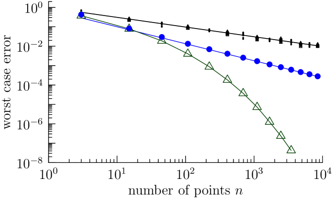
Figure 1. Integration by random sampling vs. $t$-designs. Dots refer to the worst case error in $H_{K_{1}}$, triangles to $H_{K_{2}}$. Big symbols correspond to $t_{i}$-designs, small symbols to $n_{i}$ random points. The black line is the expectation of the worst case error and has slope $-1/2$, cf. Proposition 4.5, and the blue line’s slope is $-7/8$.

To conclude this section on numerical integration, we point out that Lemma 6.1 provides analytic expressions for the worst case errors in particular reproducing kernel Hilbert spaces. If we go beyond Hilbert spaces, then numerically computing worst case errors in Sobolev spaces becomes very challenging as is illustrated by the following remark.

Remark 6.2.

Let $I_{2}$ denote the $4$ by $4$ matrix with two ones in the left upper diagonal entries and zeros elsewhere. We shall consider the integration error with respect to a sequence of low-cardinality cubatures $\{(P^{i}_{j},\omega^{i}_{j})\}_{j=1}^{n_{i}}$ for $\Pi_{t_{i}}$ in $\mathcal{G}_{2,4}$. Without loss of generality we assume $P^{i}_{1}=I_{2}$, for $i=1,2,\ldots$. The function $f_{1}(P):=K_{1}(I_{2},P)$, for $P\in\mathcal{G}_{2,4}$, is contained in $W^{7/2}_{2}(\mathcal{G}_{2,4})$, so that its integration error decays at least as fast as $n^{-7/8}$. Numerical experiments suggest that it decays exactly at this rate, so that $f_{1}$ seems to be a single representative for the worst case error of integration in the reproducing kernel Hilbert space $W^{7/2}_{2}(\mathcal{G}_{2,4})$.

Now, we point out, although $f_{1}\in W^{3}_{\infty}(\mathcal{G}_{2,4})$ with $f_{1}\not\in W^{3+\epsilon}_{\infty}(\mathcal{G}_{2,4})$, for all $\epsilon>0$, its integration error decays faster than the worst case error in $W^{3}_{\infty}(\mathcal{G}_{2,4})$, which is just $n^{-3/4}$.

6.3. Approximating covering radii by random points

Given a sequence of point sets $\{P_{j}^{i}\}_{j=1}^{n_{i}}\subset\mathcal{G}_{k,m}$, for $i=1,2,\ldots$, it is a tough task to numerically determine the exact covering radii $\rho_{i}$. In order to obtain a reasonable approximation, we generate $n\gg n_{i}$ random points $\{R_{j^{\prime}}\}_{j^{\prime}=1}^{n}\subset\mathcal{G}_{k,m}$ and determine

(30) $$\hat{\rho}_{i,n}:=\max_{1\leq j^{\prime}\leq n}\min_{1\leq j\leq n_{i}}\operatorname{dist}_{k,m}(R_{j^{\prime}},P^{i}_{j}).$$

Note that $\rho_{i}$ is sandwiched by

(31) $$\hat{\rho}_{i,n}\leq\rho_{i}\leq\hat{\rho}_{i,n}+\varrho_{n},$$

where $\varrho_{n}$ is the covering radius of the random points $\{R_{j^{\prime}}\}_{j^{\prime}=1}^{n}$. Supposed that $\varrho_{n}$ is sufficiently small, $\hat{\rho}_{i,n}$ is a decent approximation of $\rho_{i}$.

We aim to provide evidence that the computed approximation $\hat{\rho}_{i,n}$ is sufficiently accurate to numerically illustrate Theorem 3.2. To ballpark $\varrho_{n}$, recall that the covering radius $\varrho_{n}$ of $n$ random points, independently distributed according to $\mu_{k,m}$ on $\mathcal{G}_{k,m}$, behaves asymptotically as stated in (3) with $d=k(m-k)$. More precisely, [29, Corollary 3.3] yields together with the relation (25) that

(32) $$\lim_{n\rightarrow\infty}\mathbb{E}\varrho_{n}\left(\frac{n}{\log(n)}\right)^{\frac{1}{k(m-k)}}=\left(\frac{\operatorname{vol}(\mathcal{G}_{k,m})}{\operatorname{vol}(\mathbb{B}_{k(m-k)})}\right)^{\frac{1}{k(m-k)}},$$

where $\mathbb{B}_{d}$ is the unit ball in $\mathbb{R}^{d}$ and $\operatorname{vol}$ are the canonical volumes induced by the Euclidean metric. Thus, for large $n$, we expect that $\varrho_{n}$ behaves as

(33) $$\varrho_{n}\approx\left(\frac{\operatorname{vol}(\mathcal{G}_{k,m})}{\operatorname{vol}(\mathbb{B}_{k(m-k)})}\frac{n}{\log(n)}\right)^{\frac{1}{k(m-k)}}.$$

The volume of the Grassmannian is

(34) $$\operatorname{vol}(\mathcal{G}_{k,m})=\frac{\Gamma_{k}(k/2)}{\Gamma_{k}(m/2)}(2\pi)^{k(m-k)/2}$$

where $\Gamma_{k}$ is the multivariate Gamma function

$$\Gamma_{k}(x)=\pi^{k(k-1)/4}\prod_{i=1}^{k}\Gamma(x+(1-i)/2),\qquad x>\frac{1}{2}(k-1).$$

Note, the formula (34) differs by a factor of $\sqrt{2}^{k(m-k)}$ from [12, Eq. (1.4.11)] due to our additional scaling of $\sqrt{2}$ in the geodesic distance, cf. (24). The volume of $\mathbb{B}_{d}$ in $\mathbb{R}^{d}$ is

$$\operatorname{vol}(\mathbb{B}_{d})=\frac{\pi^{d/2}}{\Gamma(d/2+1)}.$$

Hence, for $k=2$, $m=4$, the expression (33) reduces to

(35) $$\varrho_{n}\approx 2n^{-\frac{1}{4}}\log(n)^{\frac{1}{4}}.$$

For $n=10^{7}$, we obtain $\varrho_{n}\approx 0.0713$, which is significantly smaller than any of the computed $\hat{\rho}_{n,i}$. According to these considerations, we argue that our numerical computations of the covering radius are sufficiently reliable in view of (31).

Figure 2 shows logarithmic plots of the estimated covering radii for the cubature points $\{P_{j}^{i}\}_{j=1}^{n_{i}}$, $i=1,\dots,14$. For comparison it also depicts estimated covering radii for random points. We observe the desired relationship $\rho_{i}\asymp n_{i}^{-1/4}$, cf. Theorem 3.2, and the estimate (35) of the expected covering radius for random points becomes more accurate for large $n$.

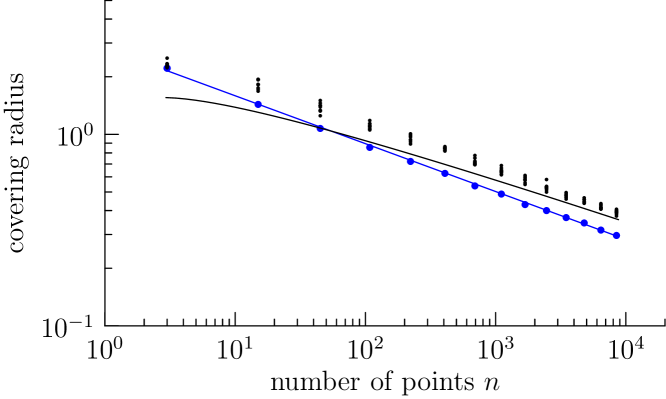
Figure 2. Covering radii of random sampling vs. $t$-designs. Big dots correspond to $t_{i}$-designs, small dots to $n_{i}$ random points. The blue line’s slope is $-1/4$. The black curve corresponds to $2n^{-\frac{1}{4}}\log(n)^{\frac{1}{4}}$, which relates to the covering radii $\varrho_{n}$ via (35).

References

- [1] P.-A. Absil, R. Mahony, and R. Sepulchre, Optimization algorithms on matrix manifolds, Princeton University Press, 2008.
- [2] C. Bachoc, Designs, groups and lattices, J. Theor. Nombres Bordeaux (2005), 25–44.
- [3] C. Bachoc, E. Bannai, and R. Coulangeon, Codes and designs in Grassmannian spaces, Discrete Mathematics 277 (2004), 15–28.
- [4] C. Bachoc, R. Coulangeon, and G. Nebe, Designs in Grassmannian spaces and lattices, J. Algebraic Combinatorics 16 (2002), 5–19.
- [5] C. Bachoc and M. Ehler, Tight -fusion frames, Appl. Comput. Harmon. Anal. 35 (2013), no. 1, 1–15.
- [6] A. Bondarenko, D. Radchenko, and M. Viazovska, Optimal asymptotic bounds for spherical designs, Ann. Math. 178 (2013), no. 2, 443–452.
- [7] L. Brandolini, C. Choirat, L. Colzani, G. Gigante, R. Seri, and G. Travaglini, Quadrature rules and distribution of points on manifolds, Annali della Scuola Normale Superiore di Pisa - Classe di Scienze XIII (2014), no. 4, 889–923.
- [8] J. Brauchart, E. Saff, I. H. Sloan, and R. Womersley, QMC designs: Optimal order quasi Monte Carlo integration schemes on the sphere, Math. Comp. 83 (2014), 2821–2851.
- [9] J. S. Brauchart, J. Dick, E. B. Saff, I. H. Sloan, Y. G. Wang, and R. S. Womersley, Covering of spheres by spherical caps and worst-case error for equal weight cubature in Sobolev spaces, J. Math. Anal. Appl. 431 (2015), no. 2, 782–811.
- [10] J. S. Brauchart and P. J. Grabner, Distributing many points on spheres: minimal energy and designs, J. Complexity 31 (2015), 293–326.
- [11] A. Breger, M. Ehler, and M. Gräf, Quasi Monte Carlo integration and kernel-based function approximation on Grassmannians, ArXiv (2016).
- [12] Y. Chikuse, Statistics on special manifolds, Lecture Notes in Statistics, Springer, New York, 2003.
- [13] C. Choirat and R. Seri, Numerical properties of generalized discrepancies on spheres of arbitrary dimension, J. Complexity 29 (2013), 216–235.
- [14] S. B. Damelin and P. J. Grabner, Energy functionals, numerical integration and asymptotic equidistribution on the sphere, J. Complexity 19 (2003), 231–246.
- [15] A. W. Davis, Spherical functions on the Grassmann manifold and generalized Jacobi polynomials - Part 2, Linear Algebra Appl. 289 (1999), no. 1-3, 95–119.
- [16] P. de la Harpe and C. Pache, Cubature formulas, geometrical designs, reproducing kernels, and Markov operators, Infinite groups: geometric, combinatorial and dynamical aspects (Basel), vol. 248, Birkhäuser, 2005, pp. 219–267.
- [17] D. Dung and T. Ullrich, Lower bounds for the integration error for multivariate functions with mixed smoothness and optimal Fibonacci cubature for functions on the square, Math. Nachr. 288 (2015), no. 7, 743–762.
- [18] M. Ehler and M. Gräf, Harmonic decompositions on unions of Grassmannians, arXiv (2016).
- [19] F. Filbir and H. N. Mhaskar, A quadrature formula for diffusion polynomials corresponding to a generalized heat kernel, J. Fourier Anal. Appl. 16 (2010), no. 5, 629–657.
- [20] by same author, Marcinkiewicz–Zygmund measures on manifolds, J. Complexity 27 (2011), no. 6, 568–596.
- [21] M. Gräf, Efficient algorithms for the computation of optimal quadrature points on Riemannian manifolds, Universitätsverlag Chemnitz, 2013.
- [22] P. Hellekalek, P. Kritzer, and F. Pillichshammer, Open type quasi-Monte Carlo integration based on Halton sequences in weighted Sobolev spaces, J. Complexity 33 (2016), 169–189.
- [23] A. Hinrichs, L. Markhasin, J. Oettershagen, and T. Ullrich, Optimal quasi-monte carlo rules on order 2 digital nets for the numerical integration of multivariate periodic functions, Numer. Math. (2015).
- [24] A. Hinrichs, E. Novak, M. Ullrich, and H. Wozniakowski, The curse of dimensionality for numerical integration of smooth functions II, J. Complexity 30 (2014), no. 2, 117–143.
- [25] L. Hörmander, The analysis of linear partial differential operators, I, II, III, IV, Springer Verlag, 1983-1985.
- [26] D. Krieg and E. Novak, A universal algorithm for multivariate integration, Found. Comput. Math. (2016).
- [27] H. Niederreiter, Some current issues in quasi-Monte Carlo methods, J. Complexity 19 (2003), no. 3, 428–433.
- [28] E. Novak and H. Wozniakowski, Tractability of Multivariate Problems. Volume II, EMS Tracts in Mathematics, vol. 12, EMS Publishing House, Zürich, 2010.
- [29] A. Reznikov and E. B. Saff, The covering radius of randomly distributed points on a manifold, International Mathematics Research Notices rnv342 (2015).
- [30] P. Seymour and T. Zaslavsky, Averaging sets: a generalization of mean values and spherical designs, Advances in Math. 52 (1984), 213–240.
- [31] I. H. Sloan and R. S. Womersley, Extremal systems of points and numerical integration on the sphere, Adv. Comput. Math. 21 (2004), 107–125.
- [32] T. Ullrich, Optimal cubature in Besov spaces with dominating mixed smoothness on the unit square, J. Complexity 30 (2014), 72–94.