High sensitivity to mass-ratio variation in deep molecular potentials

Abstract

Molecular vibrational transitions are prime candidates for model-independent searches for variation of the proton-to-electron mass ratio. Searches for present-day variation achieve highest sensitivity with deep molecular potentials. We identify several high-sensitivity transitions in the deeply bound O${}_{2}^{+}$ molecular ion. These transitions are electric-dipole forbidden and thus have narrow linewidths. The most sensitive transitions take advantage of an accidental degeneracy between vibrational states in different electronic potentials. We suggest experimentally feasible routes to a measurement with uncertainty exceeding current limits on present-day variation in $m_{p}/m_{e}$.

The dimensionless fundamental constants are the input parameters to our physical theories. Apparent variations of these constants arise naturally in many extensions to the Standard Model, including the spacetime evolution of additional dimensions or new scalar fields Uzan (2003). Recent work suggests that certain dark matter fields could induce oscillations in the values of fundamental constants Stadnik and Flambaum (2015).

The proton-to-electron mass ratio, $\mu=m_{p}/m_{e}$, is particularly interesting because the two masses arise from different mechanisms. Variation would imply a change in the relative strengths of the strong and electroweak interactions. Models typically predict the relative change of $\mu$ should be of order 40 times larger than that of the fine structure constant $\alpha$ Uzan (2003).

Searches for variation of $\mu$ have been approached over both cosmological and laboratory timescales. The current precision of cosmological searches are at the level of $10^{-6}$–$10^{-7}$ over $\sim 10^{10}$ years Kanekar (2011); Bagdonaite et al. (2013); Ubachs et al. (2016). The tightest bounds on present-day variation of $\mu$ come from atomic clock experiments, which set the limit $\dot{\mu}/\mu\lesssim 10^{-16}~{}{\rm yr}^{-1}$ Godun et al. (2014); Huntemann et al. (2014). In these experiments, nearly all the sensitivity to $\mu$ variation comes from the hyperfine structure of cesium, and extracting the precise $\mu$ dependence requires a model of the cesium nuclear magnetic moment Flambaum and Tedesco (2006).

The vibration and rotation of molecules provide a model-independent means to search for variation in $\mu$ Carr et al. (2009); Chin et al. (2009); Jansen et al. (2014). The most stringent constraint from a molecular measurement is $\dot{\mu}/\mu=(-3.8\pm 5.6)\times 10^{-14}~{}{\rm yr}^{-1}$ in SF₆ Shelkovnikov et al. (2008). We propose O${}_{2}^{+}$ as a molecule possessing a high sensitivity to present-day variation in $\mu$ as well as experimentally feasible means for measuring it. We describe two possible measurements, each of which is capable of resolving fractional changes in $\mu$ to better than $10^{-16}$ in one day with a single molecule. As discussed below, the high sensitivity arises from the molecule’s deep electronic ground-state potential (54 600 cm^-1). Other molecules with deep potentials may also have suitable transitions.

Features of the relatively simple molecular structure of O${}_{2}^{+}$ make it amenable for experiments. It is homonuclear, so nuclear symmetry eliminates half the rotational states and forbids electric dipole (E1) transitions within an electronic state. This nonpolarity suppresses many systematic effects, including some AC Stark and blackbody radiation shifts. The most common isotope of oxygen (¹⁶O, 99.8 % abundance) has no nuclear spin, so O${}_{2}^{+}$ lacks hyperfine structure. Unlike many molecular ions, O${}_{2}^{+}$ has measured spectroscopic parameters Krupenie (1972); Cosby et al. (1980); Hansen et al. (1983); Coxon and Haley (1984); Kong and Hepburn (1994, 1996); Song et al. (1999, 2000a, 2000b)  and existing theoretical calculations Fedorov et al. (1999, 2001); Zhang et al. (2011); Magrakvelidze et al. (2012); Liu et al. (2015). This prior work has been motivated in part because of the important role O${}_{2}^{+}$ plays in the ionospheres of Earth and other planets Schunk and Nagy (1980). Most relevant to the present work, several vibrational states in the middle of the O${}_{2}^{+}$ ground $X\,^{2}\Pi_{g}$ potential are nearly degenerate with low vibrational states of the excited $a\,^{4}\Pi_{u}$ potential. This degeneracy should allow searches for variation in $\mu$ with high sensitivity in both the absolute and relative senses DeMille et al. (2008).

Searches for fractional changes in $\mu$ usually involve monitoring the energy difference $\hbar\omega$ between two energies with different $\mu$-dependence, $\hbar\omega=E^{\prime}(\mu)-E^{\prime\prime}(\mu)$. The change in $\mu$ is then given by

$$\frac{\Delta\mu}{\mu}=\frac{1}{\mu}\frac{\partial\mu}{\partial\omega}\Delta\omega=\frac{\partial(\ln\mu)}{\partial\omega}\Delta\omega.$$ (1)

The absolute sensitivity of the transition is given by $\partial\omega/\partial(\ln\mu)$, which is sometimes called the absolute enhancement factor. In an experiment, the statistical precision with which $\Delta\omega$ can be measured is given by

$$\delta\omega=\frac{\Gamma}{\sqrt{M}\,S/\delta S},$$ (2)

where $\Gamma$ is the transition linewidth, $S/\delta S$ is the signal-to-noise ratio, and $M$ the number of independent measurements (assuming white noise). Here, $\delta\omega$ represents the uncertainty in determining the change $\Delta\omega$. The figure of merit is thus

$$\frac{\partial\omega}{\partial(\ln\mu)}\frac{1}{\Gamma}.$$ (3)

In some cases, such as the Doppler-broadened lines encountered in astrophysical measurements, the linewidth is proportional to the transition frequency and the figure of merit is proportional to the relative enhancement factor $[\partial\omega/\partial(\ln\mu)]/\omega$. In other cases, such as O${}_{2}^{+}$, such relative enhancement can be experimentally convenient.

Because of its importance in isotope shifts, the scaling of molecular parameters with $\mu$ has been known for some time (Herzberg, 1950, Sec. III.2.g). In particular, for a state of energy

$$E/(hc)=T_{e}+\omega_{e}(v+\tfrac{1}{2})-\omega_{e}x_{e}(v+\tfrac{1}{2})^{2}+B_{e}J(J+1),$$ (4)

the electronic energy $T_{e}$ is independent of $\mu$, the vibrational coefficient $\omega_{e}$ scales as $\mu^{-1/2}$, the lowest anharmonicity coefficient $\omega_{e}x_{e}$ scales as $\mu^{-1}$, and the rotational constant $B_{e}$ scales as $\mu^{-1}$. (Here, the parameters are given as wavenumbers. For scaling of additional coefficients, see references Herzberg (1950); Beloy et al. (2011); Pašteka et al. (2015).) Thus the absolute sensitivity of a particular state to variation in $\mu$ is given by

$$\frac{1}{hc}\frac{\partial E}{\partial(\ln\mu)}=-\tfrac{1}{2}\omega_{e}(v+\tfrac{1}{2})+\omega_{e}x_{e}(v+\tfrac{1}{2})^{2}-B_{e}J(J+1).$$ (5)

Transitions between different vibrational states will generally yield higher sensitivity both because $\omega_{e}$ tends to be larger than $B_{e}$ and because selection rules preclude transitions between states of vastly different $J$. The first term in Eq. (5) shows a linear growth in sensitivity with vibrational state. For higher states, the opposite sign of the second term slows the growth. The vibrational states return to no sensitivity near the dissociation limit. As was pointed out in refs. Zelevinsky et al. (2008); DeMille et al. (2008), the peak sensitivity is approximately 1/4 of the dissociation energy and occurs for vibrational states with energies approximately 3/4 of the dissociation limit.

Vibrational selection rules typically preclude direct transitions between low- and high-sensitivity states within the same electronic state. To alleviate this restriction, Zelevinsky et al. Zelevinsky et al. (2008) proposed driving stimulated Raman transitions via an excited electronic state and suggested Sr₂ as a candidate molecule. DeMille et al. DeMille et al. (2008) suggested transitions between different electronic states. The linewidth for such a transition can still be narrow if the inter-electronic transition is forbidden, for example by spin selection rules. DeMille et al. emphasize the practical advantage of choosing transitions with high relative sensitivity and identifies Cs₂ as a candidate molecule with a near-degeneracy between vibrational states in different-multiplicity electronic states.

Because the maximum sensitivity is proportional to the potential depth, one should look for experimentally viable routes in deeply bound molecules. We have identified O${}_{2}^{+}$ as a candidate molecule with several accessible transitions that are 50–75 times more sensitive than those in prior proposals with photoassociated molecules. Indeed, even the energy difference between the O${}_{2}^{+}$ $X\,^{2}\Pi_{g}$ ground and first-excited vibrational states has several times the absolute sensitivity of the transitions proposed in refs. Zelevinsky et al. (2008); DeMille et al. (2008). Additionally, there are accidental degeneracies between the 21^st and 22^nd excited vibrational states of the $X\,^{2}\Pi_{g}$ state and $v=0,1$ of the $a\,^{4}\Pi_{u}$ state. Several transitions between these states are likely to have energies in the microwave range. Spin-orbit coupling between $a\,^{4}\Pi_{u}$ and the nearby $A\,^{2}\Pi_{u}$ state should allow the driving of these nominally spin-forbidden transitions Lefebvre-Brion and Field (2004).

Figure 1: Potential curves (in the Morse approximation) for the $X$, $a$, and $A$ states of O${}_{2}^{+}$. The horizontal lines indicate the measured energies of vibrational states Song et al. (1999, 2000a, 2000b). Inset are the doublet-$X$ and quartet-$a$ levels discussed in the text, including spin–orbit splittings. The labels on each fine-structure level indicate $\Omega$ in the case (a) (low-$J$) limit.

The lowest molecular potentials of O${}_{2}^{+}$ have been studied for some time. Figure 1 plots the $X\,^{2}\Pi_{g}$, $a\,^{4}\Pi_{u}$, and $A\,^{2}\Pi_{u}$ potentials. The vibrational state energies have been measured up to $v=38$ for the $X$ state Kong and Hepburn (1994); Song et al. (1999), $v=18$ for the $a$ state Kong and Hepburn (1996); Song et al. (2000b), and $v=12$ for the $A$ state Song et al. (2000a). By use of the resulting molecular parameters as well as Eq. (5), we calculate each vibrational level’s sensitivity to variation in $\mu$. These sensitivities, $\partial E_{v}/\partial(\ln\mu)$, are plotted in Fig. 2. The values plotted in the figure are calculated using a Morse approximation for the potential Herzberg (1950). For the particular transitions proposed herein, the sensitivity calculated from the Morse potential and from the measured molecular parameters agree to better than 0.5 %.

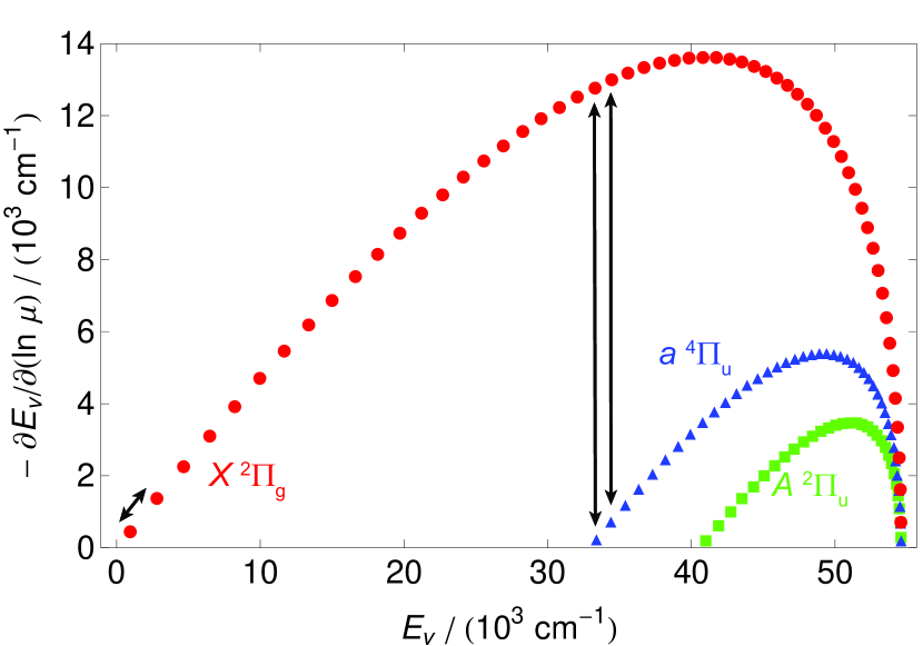
Figure 2: Absolute sensitivity of vibrational states in the $X$, $a$, and $A$ potentials, calculated using the Morse approximation. The arrows indicate the proposed transitions.

The $X$-state’s high $\omega_{e}$ means that even the lowest vibrational transitions are quite sensitive to variation in $\mu$. The transition $|X,v=0\rangle\leftrightarrow|X,v=1\rangle$, has a sensitivity of $\tfrac{1}{2\pi c}\tfrac{\partial\omega}{\partial(\ln\mu)}=920~{}{\rm cm}^{-1}=28~{}{\rm THz}/c$ and an energy difference $\Delta E/(hc)=1873~{}{\rm cm}^{-1}=1/(5339~{}{\rm nm})$. Because O${}_{2}^{+}$ is nonpolar, this transition is E1 forbidden but proceeds as an electric quadrupole (E2) transition. Its natural linewidth is thus extremely narrow and any experimental linewidth will be limited by technical noise (e.g. laser linewidth) or probe time. An experiment driving the lowest vibrational transitions with two Raman lasers has been proposed in N${}_{2}^{+}$ Kajita et al. (2014). The N${}_{2}^{+}$ ground-state $v=0\leftrightarrow 1$ electric-quadrupole transition has been driven directly with a quantum cascade laser Germann et al. (2014). Similar techniques could be applied to O${}_{2}^{+}$.

Given the absolute sensitivity, we can use Eq. (2) to estimate the achievable statistical precision of a $v=0\leftrightarrow 1$ measurement. Assuming a probe time equal to $\Gamma^{-1}$ and minimal experimental dead time, the total number of measurements scales linearly in the total measurement duration $\tau$ as $M=\tau\Gamma$. If the signal-to-noise is limited by quantum projection noise Itano et al. (1993), then $S/\delta S=\sqrt{N}$, where $N$ is the number of independent molecules probed per experimental run. The statistical precision would then be $\delta\omega\sim\sqrt{\Gamma/(N\tau)}$. With a $\Gamma/(2\pi)=1~{}{\rm Hz}$ linewidth, the lowest vibrational transition should be able to achieve $\delta\mu/\mu\sim 1.4\times 10^{-14}/\sqrt{N(\tau/{\rm sec})}$ or of order $5\times 10^{-17}$ in one day with one molecule.

To enhance sensitivity, one could measure the energy difference between vibrational states near the middle of the potential and those near the bottom or near dissociation. With a potential as deep as O${}_{2}^{+}$, driving such a transition with two Raman lasers becomes challenging. Directly driving the quadrupole overtone transitions suffers from very small quadrupole moments for large $\Delta v$. In O${}_{2}^{+}$, accidental degeneracies between different electronic potentials provide high sensitivity with relatively low energy difference. Here, two high-sensitivity states $|X\,^{2}\Pi_{g},v=21,22\rangle$ are nearly degenerate with two low-sensitivity states $|a\,^{4}\Pi_{u},v=0,1\rangle$. Figure 1(inset) shows the overlap, including spin-orbit splitting. Because the rotational coefficients of these two states are slightly different, the degeneracy may in some sense be “tuned” by choosing an appropriate $J$ and $\Delta J$. The absolute sensitivity of the $|X,v^{\prime\prime}=21\rangle\leftrightarrow|a,v^{\prime}=0\rangle$ transition is $12\,600~{}{\rm cm}^{-1}=378~{}{\rm THz}/c$; that of the $|X,v^{\prime\prime}=22\rangle\leftrightarrow|a,v^{\prime}=1\rangle$ transition is $12\,300~{}{\rm cm}^{-1}=369~{}{\rm THz}/c$. Depending on the particular $J$ and $\Delta J$, sensitivity contributions from the $B_{e}$ coefficient may be of order $100~{}{\rm cm}^{-1}$.

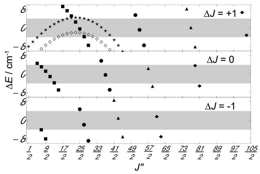
Figure 3: Degeneracy of $X$ and $a$ states. Transitions are plotted from $|X\,F_{2},v^{{\prime\prime}}=21,J^{{\prime\prime}}\rangle$ (open) or $|X\,F_{1},v^{{\prime\prime}}=21,J^{{\prime\prime}}\rangle$ (filled) to $|a\,F_{1},v^{\prime}=0,J^{\prime}\rangle$ ($\blacksquare$), $F_{2}$ (${\bullet}$), $F_{3}$ ($\blacktriangle$), or $F_{4}$ (

$\blacksquare$

). The $|X\,F_{1},v^{{\prime\prime}}=22,J^{{\prime\prime}}\rangle\leftrightarrow|a\,F_{4},v^{\prime}=1,J^{\prime}\rangle$ transitions are plotted with $\bigstar$. The separate plots indicate $\Delta J=J^{\prime\prime}-J^{\prime}=-1$, $0$, or $+1$. Gray bands show a $\pm 4~{}{\rm cm}^{-1}$ uncertainty range.

Using measured molecular parameters for the $X$ and $a$ states Hansen et al. (1983); Kong and Hepburn (1994); Song et al. (1999); Kong and Hepburn (1996), we make an effective Hamiltonian Brown and Carrington (2003) and calculate the energies and eigenstates of the individual $J$ states within the relevant vibrational states han . We calculate all transition energies with $\Delta J=0,\pm 1$ and $|\Delta E|/(hc)<10~{}{\rm cm}^{-1}=300~{}{\rm GHz}/c$. Figure 3 plots the results, which are tabulated in the Supplemental Material han . As can be seen, many energies lie in a range where radiofrequency and microwave techniques may be used. The relatively lower transition frequencies relax the demands on relative accuracy while maintaining high absolute sensitivity. The uncertainties on the calculated transition energies are 3–5 cm^-1, but they are highly correlated such that even if these particular transitions are no longer within 10 cm^-1, others will be.

While transitions between the doublet-$X$ and quartet-$a$ states are spin-forbidden, spin-orbit mixing of the $a\,^{4}\Pi_{u}$ and $A\,^{2}\Pi_{u}$ states ($7\,625~{}{\rm cm}^{-1}$ apart) provides sufficient coupling. This mixing also dominates the decay of the $a$ state and thus the linewidth of our proposed transitions. With an estimate of the mixing and the known 690 ns lifetime of the $A$ state Kuo et al. (1990), we can calculate the linewidth of each transition. Only the $a\,^{4}\Pi_{1/2,u}$ and $a\,^{4}\Pi_{3/2,u}$ substates couple to the $A$ state, so we use our effective Hamiltonian to calculate the projection of each eigenstate in the Hund’s case (a) basis. A similar technique was used in ref. Kuo et al. (1990) to explain $a$-state-lifetime data. They used $72~{}{\rm cm}^{-1}$ as an ab-initio-calculated estimate of the matrix elements $\langle a\,^{4}\Pi_{1/2,u}|H_{\rm SO}|A\,^{2}\Pi_{1/2,u}\rangle$ and $\langle a\,^{4}\Pi_{3/2,u}|H_{\rm SO}|A\,^{2}\Pi_{3/2,u}\rangle$, and we do so as well. (Ref. Minaev (1996) calculates a similar value for these matrix elements.) The transition linewidths fall in the range $\Gamma/(2\pi)=0.07\textnormal{--}10~{}{\rm Hz}$ han . With the same assumptions as before, a 1-Hz-linewidth transition should be able to achieve a statistical precision of $\delta\mu/\mu\sim 1.1\times 10^{-15}/\sqrt{N(\tau/{\rm sec})}$ or of order $4\times 10^{-18}$ in one day with one molecule.

When estimating the transition dipole moment, the same mixing of $a$ and $A$ states and spin-orbit matrix elements apply. Because the $a$ and $A$ states have similar equilibrium bond lengths, the coupling of $|X,v^{\prime\prime}\rangle$ to $|a,v^{\prime}\rangle$ is primarily through a single vibrational state $|A,v^{\prime}\rangle$. By use of RKR potential curves generated from the data in refs. Song et al. (1999, 2000a), we calculate Le Roy (2016); *leroylevel82 the Franck–Condon factor between $|X,v^{\prime\prime}=21\rangle$ and $|A,v^{\prime}=0\rangle$ to be $1.8\times 10^{-6}$. This value agrees with a prior published value Gilmore et al. (1992) that relied on older spectroscopy data to within 15 %. The electronic transition moment between $|X,v^{\prime\prime}=21\rangle$ and $|A,v^{\prime}=0\rangle$ has been calculated to be $0.503\,ea_{0}$ Gilmore et al. (1992). Combining these elements with our case (a) eigenstates, we estimate the transition dipole moment of these transitions to be of order $10^{-6}~{}ea_{0}$. A typical transition could be driven with a Rabi frequency approximately the same as its linewidth by use of a microwave electric field of order 10–100 V/m.

Straightforward techniques exist for producing and analyzing the states of O${}_{2}^{+}$. Rovibrationally selected O${}_{2}^{+}$ molecules have been produced in the $X\,^{2}\Pi_{g}$ state with $v=0,1$, and $J$ up to $\tfrac{51}{2}$ Dochain and Urbain (2015). The production is via resonance-enhanced multiphoton ionization (REMPI) with the selection coming from use of the $d\,^{1}\Pi_{g}$ Rydberg state in neutral O₂ Sur et al. (1991). Excitation to the Rydberg state requires two photons in the range 296.5–303.5 nm, and ionization requires a third photon, which could be at the same wavelength. Transfer from $|X,v=0\rangle$ to $|a,v=0\rangle$ could be driven coherently with a laser of wavelength 308 nm. This transition is allowed through the same $a$–$A$ spin-orbit mixing. The $|X,v=0\rangle\leftrightarrow|A,v=0\rangle$ transition has electric dipole moment $0.192\,ea_{0}$ Gilmore et al. (1992) and Franck–Condon factor $1.7\times 10^{-6}$. A 1 mW laser focused to $50~{}\mu$m (intensity $2.5\times 10^{5}~{}{\rm W/m}^{2}$) should produce a Rabi frequency of order 100 Hz.

Detection of the state could be done by driving from $a\,^{4}\Pi_{u}$ to $b\,^{4}\Sigma_{g}^{-}$, which has predissociation states at higher vibrational levels Hansen et al. (1982). Any population in the $|X,v=21\rangle$ state would not be transfered to the $b$ state. While preliminary measurements could take place in a beam, trapping O${}_{2}^{+}$ and sympathetic cooling to a Coulomb crystal with co-trapped atomic ions would allow longer probe times and eliminate first-order Doppler shifts. Trapping only a few atoms and molecules could enable non-destructive detection via quantum logic spectroscopy Schmidt et al. (2005); Wolf et al. (2016). Such detection could increase the duty-cycle by reducing the need to reload ions and would reduce systematic effects associated with micromotion in a radiofrequency trap Berkeland et al. (1998), though it may reduce the statistical limit because fewer molecules would be probed per experiment.

In conclusion, we have identified two routes in the O${}_{2}^{+}$ molecular ion to a high-sensitivity search for present-day variation in the proton-to-electron mass ratio. The highest sensitivity comes from an accidental degeneracy between excited vibrational levels of the $X$ state and the lowest vibrational levels of the $a$ state. We note that there is another set of degeneracies among the $|X,v=27\textnormal{--}30\rangle$, $|a,v=7\textnormal{--}10\rangle$, and $|A,v=0\textnormal{--}2\rangle$ states han . The direct overlap with the $A$ state would require a more extensive linewidth calculation than described here. It is also likely that such degeneracies exist in other molecules. Some homonuclear molecules with deep electronic-ground-state potentials and different-multiplicity potentials dipping within them include Te₂ dem , Br₂, Ge₂, and I${}_{2}^{+}$ Balasubramanian (1990). The heavier of these tend to have smaller vibrational splittings, which increase the likelihood of a degeneracy. It is possible that similar transitions can be found among the infrared-inactive vibrational modes of deeply bound nonpolar polyatomic molecules.

I Effective Hamiltonian

To calculate the energies and eigenstates of the rotational levels in a particular vibrational state, we diagonalize an effective Hamiltonian. See, for example, ref. (Brown and Carrington, 2003, Eq. 10.114–10.115). We include the electronic and vibrational state energy $T_{v}$, spin–orbit coupling $A_{v}$, and rigid-body rotation $B_{v}$. As discussed below, higher-order terms such as centrifugal distortion $D_{v}$ or $\Lambda$-doubling are not necessary at our precision.

Eigenstates in both $X\,^{2}\Pi_{g}$ and $a\,^{4}\Pi_{u}$ are written in the Hund’s case-(a) basis:

$$c_{3/2}\left|{}^{2}\Pi_{3/2}\right\rangle+c_{1/2}\left|{}^{2}\Pi_{1/2}\right\rangle$$ (S1)

$$c_{5/2}\left|{}^{4}\Pi_{5/2}\right\rangle+ c_{3/2}\left|{}^{4}\Pi_{3/2}\right\rangle+c_{1/2}\left|{}^{4}\Pi_{1/2}\right\rangle+c_{-1/2}\left|{}^{4}\Pi_{-1/2}\right\rangle.$$ (S2)

In these bases, the effective Hamiltonians are given by

$$H(^{2}\Pi)=\begin{pmatrix}T_{v}+\tfrac{A_{v}}{2}+B_{v}\left[J(J+1)-\tfrac{7}{4}\right]&-B_{v}\sqrt{J(J+1)-\tfrac{3}{4}}\\ -B_{v}\sqrt{J(J+1)-\tfrac{3}{4}}&T_{v}-\tfrac{A_{v}}{2}+B_{v}\left[J(J+1)+\tfrac{1}{4}\right]\end{pmatrix}$$ (S3)

and

$$H(^{4}\Pi)=\left(\begin{smallmatrix}T_{v}+\tfrac{3A_{v}}{2}+B_{v}\left[J(J+1)-\tfrac{19}{4}\right]&-\sqrt{3}B_{v}\sqrt{J(J+1)-\tfrac{15}{4}}&0&0\\ -\sqrt{3}B_{v}\sqrt{J(J+1)-\tfrac{15}{4}}&T_{v}+\tfrac{A_{v}}{2}+B_{v}\left[J(J+1)+\tfrac{5}{4}\right]&-2B_{v}\sqrt{J(J+1)-\tfrac{3}{4}}&0\\ 0&-2B_{v}\sqrt{J(J+1)-\tfrac{3}{4}}&T_{v}-\tfrac{A_{v}}{2}+B_{v}\left[J(J+1)+\tfrac{13}{4}\right]&-\sqrt{3}B_{v}(J+\tfrac{1}{2})\\ 0&0&-\sqrt{3}B_{v}(J+\tfrac{1}{2})&T_{v}-\tfrac{3A_{v}}{2}+B_{v}\left[J(J+1)+\tfrac{5}{4}\right]\end{smallmatrix}\right).$$ (S4)

The top-left component is the one with $\Omega=3/2$ and $5/2$, respectively.

The parameters used in these Hamiltonians are listed in Table SI. Although some identified transitions occur at fairly high $J$, the contributions of the $D_{v}$ coefficients are not important at the few-cm^-1 scale. The $D_{v}$ coefficients for the $|a\,^{4}\Pi_{u},v^{\prime}=0,1\rangle$ states are $5.0455(189)\times 10^{-6}~{}{\rm cm}^{-1}$ and $5.0567(176)\times 10^{-6}~{}{\rm cm}^{-1}$, respectively Hansen et al. (1983). We extrapolate the $D_{v}$ coefficients of the $X\,^{2}\Pi_{g}$ state from merged parameters in ref. Coxon and Haley (1984) to obtain $D_{21}=5.43(85)\times 10^{-6}~{}{\rm cm}^{-1}$ and $D_{22}=5.34(92)\times 10^{-6}~{}{\rm cm}^{-1}$. Even at the higher $J$’s, the contributions from $D_{v}$ cancel to be consistent with zero with uncertainties of a few times $0.1~{}{\rm cm}^{-1}$.

Table SI: Coefficients used in energy calculations. Uncertainties are shown in parentheses.

state	$T_{v}/{\rm cm}^{-1}$	$A_{v}/{\rm cm}^{-1}$	$B_{v}/{\rm cm}^{-1}$
$X\,^{2}\Pi_{g},v=21$	$129896.9(2.0)$	$177.0(1.0)$	1.25(3)
$X\,^{2}\Pi_{g},v=22$	$131075(5)$	$174.0(1.0)$	1.25(1)
$a\,^{4}\Pi_{u},v=0$	$129892(2)$	$-47.7927(19)$	$1.096990(26)$
$a\,^{4}\Pi_{u},v=1$	$130904(2)$	$-47.7997(21)$	$1.081532(18)$

II Tables of near-degeneracies

Below are tables listing every pair of energy levels with $|\Delta E|<10~{}{\rm cm}^{-1}$ and $\Delta J=0,\pm 1$. Also provided are the estimated linewidths and the eigenstate superposition coefficients from diagonalizing the effective Hamiltonians above. The uncertainties in $\Delta E$ are 3–6 ${\rm cm}^{-1}$. They are highly correlated, however, such that even if these particular transitions are no longer within $10~{}{\rm cm}^{-1}$, others likely will be. By convention Herzberg (1950); Brown and Carrington (2003), the $F_{i}$ indicate the energy order of the eigenstates for a given $J$ with $F_{1}$ having the lowest energy. In the case (a) limit, the O${}_{2}^{+}$ $X\,^{2}\Pi_{g}$ state has $\Omega=\tfrac{1}{2}$ in $F_{1}$ and $\tfrac{3}{2}$ in $F_{2}$, while the $a\,^{4}\Pi_{u}$ state has $\Omega=\tfrac{5}{2},\tfrac{3}{2},\tfrac{1}{2},-\tfrac{1}{2}$ in $F_{1,2,3,4}$.

Table SII: The near-degeneracies $|X\,^{2}\Pi_{g},v^{\prime\prime}=21,J^{\prime\prime}\rangle$ and $|a\,^{4}\Pi_{u},v^{\prime}=0,J^{\prime}\rangle$, including the eigenstate superposition coefficients.

$X\,^{2}\Pi_{g}$	$a\,^{4}\Pi_{u}$	$J^{\prime\prime}$	$J^{\prime}$	$\Delta E/{\rm cm}^{-1}$	$\frac{\Gamma}{2\pi}/{\rm Hz}$	$c_{3/2}^{{\prime\prime}}$	$c_{1/2}^{\prime\prime}$	$c_{5/2}^{\prime}$	$c_{3/2}^{\prime}$	$c_{1/2}^{\prime}$	$c_{-1/2}^{\prime}$
$F_{2}$	$F_{4}$	$\frac{7}{2}$	$\frac{9}{2}$	$-8.88$	$0.45$	$-1.00$	$0.03$	$-0.00$	$0.02$	$-0.20$	$0.98$
$F_{2}$	$F_{4}$	$\frac{9}{2}$	$\frac{11}{2}$	$-7.30$	$0.63$	$-1.00$	$0.04$	$-0.00$	$0.03$	$-0.24$	$0.97$
$F_{2}$	$F_{4}$	$\frac{11}{2}$	$\frac{13}{2}$	$-5.91$	$0.83$	$-1.00$	$0.04$	$-0.00$	$0.04$	$-0.27$	$0.96$
$F_{2}$	$F_{4}$	$\frac{13}{2}$	$\frac{15}{2}$	$-4.71$	$1.05$	$-1.00$	$0.05$	$-0.01$	$0.05$	$-0.30$	$0.95$
$F_{2}$	$F_{4}$	$\frac{15}{2}$	$\frac{17}{2}$	$-3.71$	$1.28$	$-1.00$	$0.06$	$-0.01$	$0.07$	$-0.34$	$0.94$
$F_{2}$	$F_{4}$	$\frac{17}{2}$	$\frac{19}{2}$	$-2.91$	$1.52$	$-1.00$	$0.06$	$-0.01$	$0.08$	$-0.36$	$0.93$
$F_{2}$	$F_{4}$	$\frac{19}{2}$	$\frac{21}{2}$	$-2.32$	$1.77$	$-1.00$	$0.07$	$-0.01$	$0.09$	$-0.39$	$0.92$
$F_{2}$	$F_{4}$	$\frac{21}{2}$	$\frac{23}{2}$	$-1.95$	$2.02$	$-1.00$	$0.08$	$-0.01$	$0.11$	$-0.42$	$0.90$
$F_{2}$	$F_{4}$	$\frac{23}{2}$	$\frac{25}{2}$	$-1.80$	$2.27$	$-1.00$	$0.08$	$-0.02$	$0.12$	$-0.44$	$0.89$
$F_{2}$	$F_{4}$	$\frac{25}{2}$	$\frac{27}{2}$	$-1.88$	$2.52$	$-1.00$	$0.09$	$-0.02$	$0.13$	$-0.46$	$0.88$
$F_{2}$	$F_{4}$	$\frac{27}{2}$	$\frac{29}{2}$	$-2.19$	$2.76$	$-1.00$	$0.10$	$-0.03$	$0.15$	$-0.48$	$0.86$
$F_{2}$	$F_{4}$	$\frac{29}{2}$	$\frac{31}{2}$	$-2.74$	$3.00$	$-0.99$	$0.11$	$-0.03$	$0.16$	$-0.50$	$0.85$
$F_{2}$	$F_{4}$	$\frac{31}{2}$	$\frac{33}{2}$	$-3.54$	$3.23$	$-0.99$	$0.11$	$-0.03$	$0.18$	$-0.51$	$0.84$
$F_{2}$	$F_{4}$	$\frac{33}{2}$	$\frac{35}{2}$	$-4.60$	$3.45$	$-0.99$	$0.12$	$-0.04$	$0.19$	$-0.53$	$0.83$
$F_{2}$	$F_{4}$	$\frac{35}{2}$	$\frac{37}{2}$	$-5.90$	$3.66$	$-0.99$	$0.13$	$-0.04$	$0.20$	$-0.54$	$0.81$
$F_{2}$	$F_{4}$	$\frac{37}{2}$	$\frac{39}{2}$	$-7.47$	$3.87$	$-0.99$	$0.13$	$-0.05$	$0.21$	$-0.55$	$0.80$
$F_{2}$	$F_{4}$	$\frac{39}{2}$	$\frac{41}{2}$	$-9.30$	$4.07$	$-0.99$	$0.14$	$-0.05$	$0.23$	$-0.57$	$0.79$
$F_{1}$	$F_{1}$	$\frac{7}{2}$	$\frac{5}{2}$	$-3.90$	$0.07$	$-0.03$	$-1.00$	$1.00$	$0.08$	$0.00$	$0.00$
$F_{1}$	$F_{1}$	$\frac{9}{2}$	$\frac{7}{2}$	$-7.85$	$0.16$	$-0.04$	$-1.00$	$0.99$	$0.12$	$0.01$	$0.00$
$F_{1}$	$F_{1}$	$\frac{5}{2}$	$\frac{5}{2}$	$4.79$	$0.07$	$-0.02$	$-1.00$	$1.00$	$0.08$	$0.00$	$0.00$
$F_{1}$	$F_{1}$	$\frac{7}{2}$	$\frac{7}{2}$	$3.32$	$0.16$	$-0.03$	$-1.00$	$0.99$	$0.12$	$0.01$	$0.00$
$F_{1}$	$F_{1}$	$\frac{9}{2}$	$\frac{9}{2}$	$1.43$	$0.27$	$-0.04$	$-1.00$	$0.99$	$0.16$	$0.02$	$0.00$
$F_{1}$	$F_{1}$	$\frac{11}{2}$	$\frac{11}{2}$	$-0.87$	$0.41$	$-0.04$	$-1.00$	$0.98$	$0.19$	$0.02$	$0.00$
$F_{1}$	$F_{1}$	$\frac{13}{2}$	$\frac{13}{2}$	$-3.59$	$0.57$	$-0.05$	$-1.00$	$0.97$	$0.23$	$0.03$	$0.00$
$F_{1}$	$F_{1}$	$\frac{15}{2}$	$\frac{15}{2}$	$-6.71$	$0.74$	$-0.06$	$-1.00$	$0.97$	$0.26$	$0.04$	$0.00$
$F_{1}$	$F_{1}$	$\frac{17}{2}$	$\frac{19}{2}$	$9.42$	$1.12$	$-0.06$	$-1.00$	$0.95$	$0.31$	$0.06$	$0.01$
$F_{1}$	$F_{1}$	$\frac{19}{2}$	$\frac{21}{2}$	$7.57$	$1.33$	$-0.07$	$-1.00$	$0.94$	$0.34$	$0.08$	$0.01$
$F_{1}$	$F_{1}$	$\frac{21}{2}$	$\frac{23}{2}$	$5.34$	$1.55$	$-0.08$	$-1.00$	$0.93$	$0.37$	$0.09$	$0.01$
$F_{1}$	$F_{1}$	$\frac{23}{2}$	$\frac{25}{2}$	$2.72$	$1.76$	$-0.08$	$-1.00$	$0.92$	$0.39$	$0.10$	$0.02$
$F_{1}$	$F_{1}$	$\frac{25}{2}$	$\frac{27}{2}$	$-0.28$	$1.99$	$-0.09$	$-1.00$	$0.90$	$0.41$	$0.11$	$0.02$
$F_{1}$	$F_{1}$	$\frac{27}{2}$	$\frac{29}{2}$	$-3.67$	$2.21$	$-0.10$	$-1.00$	$0.89$	$0.43$	$0.13$	$0.02$
$F_{1}$	$F_{1}$	$\frac{29}{2}$	$\frac{31}{2}$	$-7.42$	$2.43$	$-0.11$	$-0.99$	$0.88$	$0.45$	$0.14$	$0.03$
$F_{1}$	$F_{2}$	$\frac{25}{2}$	$\frac{23}{2}$	$4.95$	$9.38$	$-0.09$	$-1.00$	$-0.36$	$0.82$	$0.44$	$0.10$
$F_{1}$	$F_{2}$	$\frac{27}{2}$	$\frac{25}{2}$	$-1.75$	$9.16$	$-0.10$	$-1.00$	$-0.39$	$0.79$	$0.46$	$0.11$
$F_{1}$	$F_{2}$	$\frac{29}{2}$	$\frac{27}{2}$	$-8.77$	$8.93$	$-0.11$	$-0.99$	$-0.41$	$0.76$	$0.48$	$0.13$
$F_{1}$	$F_{2}$	$\frac{35}{2}$	$\frac{35}{2}$	$5.91$	$8.04$	$-0.13$	$-0.99$	$-0.48$	$0.66$	$0.55$	$0.18$
$F_{1}$	$F_{2}$	$\frac{37}{2}$	$\frac{37}{2}$	$-0.21$	$7.82$	$-0.13$	$-0.99$	$-0.50$	$0.63$	$0.56$	$0.19$
$F_{1}$	$F_{2}$	$\frac{39}{2}$	$\frac{39}{2}$	$-6.63$	$7.61$	$-0.14$	$-0.99$	$0.51$	$-0.60$	$-0.58$	$-0.21$
$F_{1}$	$F_{2}$	$\frac{51}{2}$	$\frac{53}{2}$	$5.66$	$6.33$	$-0.18$	$-0.98$	$-0.58$	$0.44$	$0.62$	$0.29$
$F_{1}$	$F_{2}$	$\frac{53}{2}$	$\frac{55}{2}$	$-0.72$	$6.18$	$-0.18$	$-0.98$	$-0.59$	$0.42$	$0.62$	$0.30$
$F_{1}$	$F_{2}$	$\frac{55}{2}$	$\frac{57}{2}$	$-7.39$	$6.04$	$-0.19$	$-0.98$	$0.60$	$-0.40$	$-0.63$	$-0.30$
$F_{1}$	$F_{3}$	$\frac{41}{2}$	$\frac{39}{2}$	$8.89$	$7.13$	$-0.15$	$-0.99$	$-0.19$	$0.57$	$-0.57$	$-0.56$
$F_{1}$	$F_{3}$	$\frac{43}{2}$	$\frac{41}{2}$	$1.14$	$6.94$	$-0.15$	$-0.99$	$0.21$	$-0.58$	$0.55$	$0.57$
$F_{1}$	$F_{3}$	$\frac{45}{2}$	$\frac{43}{2}$	$-6.87$	$6.76$	$-0.16$	$-0.99$	$-0.22$	$0.59$	$-0.52$	$-0.58$
$F_{1}$	$F_{3}$	$\frac{57}{2}$	$\frac{57}{2}$	$2.66$	$5.71$	$-0.20$	$-0.98$	$0.29$	$-0.62$	$0.37$	$0.63$
$F_{1}$	$F_{3}$	$\frac{59}{2}$	$\frac{59}{2}$	$-5.06$	$5.58$	$-0.20$	$-0.98$	$-0.30$	$0.62$	$-0.35$	$-0.63$
$F_{1}$	$F_{3}$	$\frac{75}{2}$	$\frac{77}{2}$	$8.43$	$4.74$	$-0.25$	$-0.97$	$0.37$	$-0.62$	$0.21$	$0.66$
$F_{1}$	$F_{3}$	$\frac{77}{2}$	$\frac{79}{2}$	$0.36$	$4.67$	$-0.25$	$-0.97$	$-0.37$	$0.62$	$-0.20$	$-0.66$
$F_{1}$	$F_{3}$	$\frac{79}{2}$	$\frac{81}{2}$	$-7.99$	$4.60$	$-0.26$	$-0.97$	$0.38$	$-0.62$	$0.18$	$0.66$
$F_{1}$	$F_{4}$	$\frac{61}{2}$	$\frac{59}{2}$	$1.74$	$5.45$	$-0.21$	$-0.98$	$-0.09$	$0.32$	$-0.63$	$0.70$
$F_{1}$	$F_{4}$	$\frac{63}{2}$	$\frac{61}{2}$	$-6.89$	$5.57$	$-0.21$	$-0.98$	$0.09$	$-0.33$	$0.63$	$-0.69$
$F_{1}$	$F_{4}$	$\frac{79}{2}$	$\frac{79}{2}$	$3.89$	$6.38$	$-0.26$	$-0.97$	$0.13$	$-0.39$	$0.66$	$-0.63$
$F_{1}$	$F_{4}$	$\frac{81}{2}$	$\frac{81}{2}$	$-4.98$	$6.45$	$-0.26$	$-0.96$	$0.13$	$-0.39$	$0.66$	$-0.63$
$F_{1}$	$F_{4}$	$\frac{101}{2}$	$\frac{103}{2}$	$6.82$	$7.01$	$-0.31$	$-0.95$	$0.16$	$-0.44$	$0.67$	$-0.58$
$F_{1}$	$F_{4}$	$\frac{103}{2}$	$\frac{105}{2}$	$-2.97$	$7.05$	$-0.31$	$-0.95$	$0.17$	$-0.44$	$0.67$	$-0.57$

Table SIII: The near-degeneracies $|X\,^{2}\Pi_{g},v^{\prime\prime}=22,J^{\prime\prime}\rangle$ and $|a\,^{4}\Pi_{u},v^{\prime}=1,J^{\prime}\rangle$, including the eigenstate superposition coefficients.

$X\,^{2}\Pi_{g}$	$a\,^{4}\Pi_{u}$	$J^{\prime\prime}$	$J^{\prime}$	$\Delta E/{\rm cm}^{-1}$	$\frac{\Gamma}{2\pi}/{\rm Hz}$	$c_{3/2}^{{\prime\prime}}$	$c_{1/2}^{\prime\prime}$	$c_{5/2}^{\prime}$	$c_{3/2}^{\prime}$	$c_{1/2}^{\prime}$	$c_{-1/2}^{\prime}$
$F_{1}$	$F_{4}$	$\frac{1}{2}$	$\frac{3}{2}$	$-7.84$	$0.08$	$0.00$	$1.00$	$0.00$	$0.00$	$-0.08$	$1.00$
$F_{1}$	$F_{4}$	$\frac{3}{2}$	$\frac{5}{2}$	$-5.77$	$0.17$	$-0.01$	$-1.00$	$-0.00$	$0.01$	$-0.12$	$0.99$
$F_{1}$	$F_{4}$	$\frac{5}{2}$	$\frac{7}{2}$	$-3.87$	$0.30$	$-0.02$	$-1.00$	$-0.00$	$0.01$	$-0.16$	$0.99$
$F_{1}$	$F_{4}$	$\frac{7}{2}$	$\frac{9}{2}$	$-2.15$	$0.45$	$-0.03$	$-1.00$	$-0.00$	$0.02$	$-0.20$	$0.98$
$F_{1}$	$F_{4}$	$\frac{9}{2}$	$\frac{11}{2}$	$-0.61$	$0.63$	$-0.04$	$-1.00$	$-0.00$	$0.03$	$-0.23$	$0.97$
$F_{1}$	$F_{4}$	$\frac{11}{2}$	$\frac{13}{2}$	$0.75$	$0.84$	$-0.04$	$-1.00$	$-0.00$	$0.04$	$-0.27$	$0.96$
$F_{1}$	$F_{4}$	$\frac{13}{2}$	$\frac{15}{2}$	$1.92$	$1.06$	$-0.05$	$-1.00$	$-0.00$	$0.05$	$-0.30$	$0.95$
$F_{1}$	$F_{4}$	$\frac{15}{2}$	$\frac{17}{2}$	$2.90$	$1.30$	$-0.06$	$-1.00$	$-0.01$	$0.06$	$-0.33$	$0.94$
$F_{1}$	$F_{4}$	$\frac{17}{2}$	$\frac{19}{2}$	$3.67$	$1.55$	$-0.06$	$-1.00$	$-0.01$	$0.08$	$-0.36$	$0.93$
$F_{1}$	$F_{4}$	$\frac{19}{2}$	$\frac{21}{2}$	$4.24$	$1.80$	$-0.07$	$-1.00$	$-0.01$	$0.09$	$-0.39$	$0.92$
$F_{1}$	$F_{4}$	$\frac{21}{2}$	$\frac{23}{2}$	$4.59$	$2.06$	$-0.08$	$-1.00$	$-0.01$	$0.10$	$-0.41$	$0.91$
$F_{1}$	$F_{4}$	$\frac{23}{2}$	$\frac{25}{2}$	$4.73$	$2.31$	$-0.09$	$-1.00$	$-0.02$	$0.12$	$-0.44$	$0.89$
$F_{1}$	$F_{4}$	$\frac{25}{2}$	$\frac{27}{2}$	$4.63$	$2.57$	$-0.09$	$-1.00$	$-0.02$	$0.13$	$-0.46$	$0.88$
$F_{1}$	$F_{4}$	$\frac{27}{2}$	$\frac{29}{2}$	$4.31$	$2.82$	$-0.10$	$-0.99$	$-0.02$	$0.14$	$-0.48$	$0.87$
$F_{1}$	$F_{4}$	$\frac{29}{2}$	$\frac{31}{2}$	$3.74$	$3.06$	$-0.11$	$-0.99$	$-0.03$	$0.16$	$-0.49$	$0.85$
$F_{1}$	$F_{4}$	$\frac{31}{2}$	$\frac{33}{2}$	$2.93$	$3.30$	$-0.11$	$-0.99$	$-0.03$	$0.17$	$-0.51$	$0.84$
$F_{1}$	$F_{4}$	$\frac{33}{2}$	$\frac{35}{2}$	$1.87$	$3.53$	$-0.12$	$-0.99$	$-0.04$	$0.18$	$-0.53$	$0.83$
$F_{1}$	$F_{4}$	$\frac{35}{2}$	$\frac{37}{2}$	$0.56$	$3.75$	$-0.13$	$-0.99$	$-0.04$	$0.20$	$-0.54$	$0.82$
$F_{1}$	$F_{4}$	$\frac{37}{2}$	$\frac{39}{2}$	$-1.01$	$3.97$	$-0.13$	$-0.99$	$0.04$	$-0.21$	$0.55$	$-0.81$
$F_{1}$	$F_{4}$	$\frac{39}{2}$	$\frac{41}{2}$	$-2.85$	$4.17$	$-0.14$	$-0.99$	$0.05$	$-0.22$	$0.56$	$-0.79$
$F_{1}$	$F_{4}$	$\frac{41}{2}$	$\frac{43}{2}$	$-4.95$	$4.36$	$-0.15$	$-0.99$	$-0.05$	$0.23$	$-0.57$	$0.78$
$F_{1}$	$F_{4}$	$\frac{43}{2}$	$\frac{45}{2}$	$-7.32$	$4.55$	$-0.15$	$-0.99$	$-0.06$	$0.25$	$-0.58$	$0.77$
$F_{1}$	$F_{4}$	$\frac{45}{2}$	$\frac{47}{2}$	$-9.97$	$4.73$	$-0.16$	$-0.99$	$-0.06$	$0.26$	$-0.59$	$0.76$

III Other degeneracies

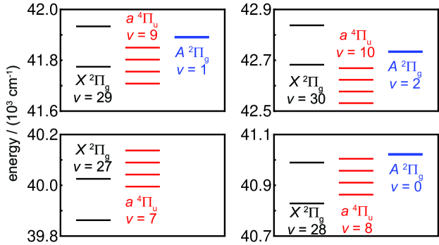
Figure S1: Overlap of the $X\,^{2}\Pi_{g}$, $a\,^{4}\Pi_{u}$, and $A\,^{2}\Pi_{u}$ states near $|X,v=27\textnormal{--}30\rangle$. The levels are calculated from refs. Song et al. (1999, 2000a, 2000b). Note that the $A$ state’s spin-orbit constant is small enough that the doublet splitting is not visible at this scale.

References

Uzan (2003)Jean-Philippe Uzan, “The
fundamental constants and their variation: observational and theoretical
status,” Rev. Mod. Phys. 75, 403–455 (2003).
Stadnik and Flambaum (2015)Y. V. Stadnik and V. V. Flambaum, “Can dark
matter induce cosmological evolution of the fundamental constants of
nature?” Phys. Rev. Lett. 115, 201301 (2015).
Kanekar (2011)Nissim Kanekar, “Constraining
changes in the proton-electron mass ratio with inversion and rotation
lines,” Astrophys. J. Lett. 728, L12 (2011).
Bagdonaite et al. (2013)J. Bagdonaite, M. Daprà, P. Jansen,
H. L. Bethlem, W. Ubachs, S. Muller, C. Henkel, and K. M. Menten, “Robust constraint on a drifting proton-to-electron mass ratio at
from methanol observation at three radio telescopes,” Phys. Rev. Lett. 111, 231101 (2013).
Ubachs et al. (2016)W. Ubachs, J. Bagdonaite,
E. J. Salumbides,
M. T. Murphy, and L. Kaper, “Colloquium: Search for a drifting
proton-electron mass ratio from H2,” Rev. Mod. Phys. 88, 021003 (2016).
Godun et al. (2014)R. M. Godun, P. B. R. Nisbet-Jones, J. M. Jones, S. A. King,
L. A. M. Johnson,
H. S. Margolis, K. Szymaniec, S. N. Lea, K. Bongs, and P. Gill, “Frequency ratio of two optical clock transitions in 171Yb+ and
constraints on the time variation of fundamental constants,” Phys. Rev. Lett. 113, 210801 (2014).
Huntemann et al. (2014)N. Huntemann, B. Lipphardt, Chr. Tamm,
V. Gerginov, S. Weyers, and E. Peik, “Improved limit on a temporal variation of from
comparisons of Yb+ and Cs atomic clocks,” Phys. Rev. Lett. 113, 210802 (2014).
Flambaum and Tedesco (2006)V. V. Flambaum and A. F. Tedesco, “Dependence of
nuclear magnetic moments on quark masses and limits on temporal variation of
fundamental constants from atomic clock experiments,” Phys.
Rev. C 73, 055501
(2006).
Carr et al. (2009)Lincoln D. Carr, David DeMille, Roman V. Krems, and Jun Ye, “Cold and ultracold
molecules: science, technology, and applications,” New J. Phys. 11, 055049
(2009).
Chin et al. (2009)Cheng Chin, V. V. Flambaum,
and M. G. Kozlov, “Ultracold molecules: new
probes on the variation of fundamental constants,” New J. Phys. 11, 055048
(2009).
Jansen et al. (2014)Paul Jansen, Hendrick L. Bethlem, and Wim Ubachs, “Perspective:
Tipping the scales: Search for drifting constants from molecular spectra,” J. Chem. Phys. 140, 010901 (2014).
Shelkovnikov et al. (2008)A. Shelkovnikov, R. J. Butcher, C. Chardonnet,
and A. Amy-Klein, “Stability of the
proton-to-electron mass ratio,” Phys. Rev. Lett. 100, 150801 (2008).
Cosby et al. (1980)P. C. Cosby, J.-B. Ozenne,
J. T. Moseley, and D. L. Albritton, “High-resolution
photofragment spectroscopy of the O first negative
system using coaxial dye-laser and velocity-tuned ion beams,” J. Mol. Spec. 79, 203–235 (1980).
Hansen et al. (1983)J. C. Hansen, J. T. Moseley,
and P. C. Cosby, “High-resolution
photofragment spectroscopy of the O first negative
system,” J. Mol. Spec. 98, 48–63 (1983).
Coxon and Haley (1984)J. A. Coxon and M. P. Haley, “Rotational
analysis of the second negative band
system of 16O,” J. Mol. Spec. 108, 119–136 (1984).
Kong and Hepburn (1994)W. Kong and J. W. Hepburn, “Rotationally
resolved threshold photoelectron spectroscopy of O2 using coherent
XUV: formation of vibrationally excited ions in the Franck–Condon
gap,” Can. J. Phys. 72, 1284–1293 (1994).
Song et al. (1999)Y. Song, M. Evans,
C. Y. Ng, C.-W. Hsu, and G. K. Jarvis, “Rotationally resolved pulsed field ionization
photoelectron bands of O() in the
energy range of eV,” J. Chem. Phys. 111, 1905–1916 (1999).
Song et al. (2000a)Y. Song, M. Evans,
C. Y. Ng, C.-W. Hsu, and G. K. Jarvis, “Rotationally resolved pulsed-field ionization
photoelectron bands of O() in the energy
range of eV,” J. Chem. Phys. 112, 1271–1278 (2000a).
Song et al. (2000b)Y. Song, M. Evans,
C. Y. Ng, C.-W. Hsu, and G. K. Jarvis, “Rotationally resolved pulsed field ionization
photoelectron bands of O() in the energy
range of eV,” J. Chem. Phys. 112, 1306–1315 (2000b).
Fedorov et al. (1999)D. G. Fedorov, M. Evans,
Y. Song, M. S. Gordon, and C. Y. Ng, “An experimental and theoretical study of the spin-orbit
interaction for CO+ () and O),” J. Chem. Phys. 111, 6413–6421 (1999).
Fedorov et al. (2001)D. G. Fedorov, M. S. Gordon,
Y. Song, and C. Y. Ng, “Theoretical study of spin-orbit coupling
constants for O and
,” J. Chem.
Phys. 115, 7393–7400
(2001).
Zhang et al. (2011)Xiaoniu Zhang, Deheng Shi,
Jinfeng Sun, and Zunlue Zhu, “MRCI study of spectroscopic and
molecular properties of X, a, A, b,
D and B electronic states of O ion,” Mol. Phys. 109, 1627–1638 (2011).
Magrakvelidze et al. (2012)M. Magrakvelidze, C. M. Aikens, and U. Thumm, “Dissociation
dynamics of diatomic molecules in intense laser fields: A scheme for the
selection of relevant adiabatic potential curves,” Phys.
Rev. A 86, 023402
(2012).
Liu et al. (2015)Hui Liu, Deheng Shi,
Jinfeng Sun, and Zunlue Zhu, “Accurate theoretical investigations of
the 20 -S and 58 states of O cation including
spin–orbit coupling effect,” Mol. Phys. 113, 120–136 (2015).
DeMille et al. (2008)D. DeMille, S. Sainis,
J. Sage, T. Bergeman, S. Kotochigova, and E. Tiesinga, “Enhanced sensitivity to variation of in
molecular spectra,” Phys. Rev. Lett. 100, 043202 (2008).
Herzberg (1950)Gerhard Herzberg, Molecular Spectra and
Molecular Structure, Vol. I: Spectra of Diatomic Molecules (D. Van Nostrand Co., 1950).
Beloy et al. (2011)K. Beloy, M. G. Kozlov,
A. Borschevsky, A. W. Hauser, V. V. Flambaum, and P. Schwerdtfeger, “Rotational spectrum of the molecular ion
NH+ as a probe for and variation,” Phys.
Rev. A 83, 062514
(2011).
Pašteka et al. (2015)L. F. Pašteka, A. Borschevsky, V. V. Flambaum, and P. Schwerdtfeger, “Search
for the variation of fundamental constants: Strong enhancements in
cations of dihalogens and hydrogen halides,” Phys.
Rev. A 92, 012103
(2015).
Zelevinsky et al. (2008)T. Zelevinsky, S. Kotochigova, and Jun Ye, “Precision test of
mass-ratio variations with lattice-confined ultracold molecules,” Phys. Rev. Lett. 100, 043201 (2008).
Lefebvre-Brion and Field (2004)Hélène Lefebvre-Brion and Robert W. Field, The Spectra and Dynamics of Diatomic Molecules (Elsevier, 2004).
Kajita et al. (2014)Masatoshi Kajita, Geetha Gopakumar, Minori Abe, Masahiko Hada, and Matthias Keller, “Test of changes using vibrational transitions in N,” Phys. Rev. A 89, 032509 (2014).
Germann et al. (2014)Matthias Germann, Xin Tong, and Stefan Willitsch, “Observation
of electric-dipole-forbidden infrared transitions in cold molecular ions,” Nature Phys. 10, 820–824 (2014).
Itano et al. (1993)W. M. Itano, J. C. Bergquist, J. J. Bollinger, J. M. Gilligan, D. J. Heinzen, F. L. Moore,
M. G. Raizen, and D. J. Wineland, “Quantum projection noise:
Population fluctuations in two-level systems,” Phys.
Rev. A 47, 3554–3570
(1993).
Brown and Carrington (2003)John Brown and Alan Carrington, Rotational
Spectroscopy of Diatomic Molecules (Cambridge
University Press, 2003).
(38)See Supplemental Material for additional
calculations, data tables, and figures.
Kuo et al. (1990)Chau-Hong Kuo, Thomas Wyttenbach, Cindy G. Beggs, Paul R. Kemper,
and Michael T. Bowers, “Radiative
lifetimes of metatable and ,” J. Chem. Phys. 92, 4849–4855 (1990).
Minaev (1996)B. F. Minaev, “Calculation of
the transition intensity in the O ion,” Optika i
spektroskopiya 80, 407–412 (1996).
Le Roy (2016)R. J. Le Roy, RKR1 2.1: A Computer Program Implementing the First-Order RKR
Method for Determining Diatomic Molecule Potential Energy Functions, University of Waterloo Chemical Physics Research
Report CP-657R (2016).
Le Roy (2014)R. J. Le Roy, LEVEL 8.2: A Computer Program for Solving the Radial
Schrödinger Equation for Bound and Quasibound Levels, University of Waterloo Chemical Physics Research Report
CP-668 (2014), see
http://leroy.waterloo.ca/programs/.
Gilmore et al. (1992)Forrest R. Gilmore, Russ R. Laher, and Patrick J. Espy, “Franck-Condon factors, -centroids, electronic transition moments, and
Einstein coefficients for many nitrogen and oxygen band systems,” J.
Phys. Chem. Ref. Data 21, 1005–1107 (1992).
Dochain and Urbain (2015)A. Dochain and X. Urbain, “Production of a
rovibrationally selected beam for dissociative recombination
studies,” EPJ Web of Conferences 84, 05001 (2015).
Sur et al. (1991)Abha Sur, R. S. Friedman, and Paul J. Miller, “Rotational dependence of the
Rydberg-valence interactions in the states of molecular
oxygen,” J. Chem. Phys. 94, 1705–1711 (1991).
Hansen et al. (1982)J. C. Hansen, J. T. Moseley,
A. L. Roche, and P. C. Cosby, “Lifetimes and predissociation mechanisms
of O,” J. Chem. Phys. 77, 1206–1213 (1982).
Schmidt et al. (2005)P. O. Schmidt, T. Rosenband,
C. Langer, W. M. Itano, J. C. Bergquist, and D. J. Wineland, “Spectroscopy using quantum logic,” Science 309, 749–752
(2005).
Wolf et al. (2016)Fabian Wolf, Yong Wan,
Jan C. Heip, Florian Gerbert, Chunyan Shi, and Piet O. Schmidt, “Non-destructive state detection for quantum
logic spectroscopy of molecular ions,” Nature 530, 457–460 (2016).
Berkeland et al. (1998)D. J. Berkeland, J. D. Miller, J. C. Bergquist, W. M. Itano, and D. J. Wineland, “Minimization
of ion micromotion in a Paul trap,” J. Appl. Phys. 83, 5025–5033 (1998).
(50)D. DeMille and M. G. Kozlov (private
communication).
Balasubramanian (1990)K. Balasubramanian, “Spectroscopic constants and potential energy curves of heavy p-block
dimers and trimers,” Chem. Rev. 90, 93–167 (1990).
Supplemental Material: High sensitivity to mass-ratio variation
in deep molecular potentialsD. Hanneke, R. A. Carollo, and D. A. Lane
Physics & Astronomy Department, Amherst College, Amherst, Massachusetts 01002, USA

References

Brown and Carrington (2003)John Brown and Alan Carrington, Rotational
Spectroscopy of Diatomic Molecules (Cambridge
University Press, 2003).
Hansen et al. (1983)J. C. Hansen, J. T. Moseley,
and P. C. Cosby, “High-resolution
photofragment spectroscopy of the O first negative
system,” J. Mol. Spec. 98, 48–63 (1983).
Coxon and Haley (1984)J. A. Coxon and M. P. Haley, “Rotational
analysis of the second negative band
system of 16O,” J. Mol. Spec. 108, 119–136 (1984).
Kong and Hepburn (1994)W. Kong and J. W. Hepburn, “Rotationally
resolved threshold photoelectron spectroscopy of O2 using coherent
XUV: formation of vibrationally excited ions in the Franck–Condon
gap,” Can. J. Phys. 72, 1284–1293 (1994).
Song et al. (1999)Y. Song, M. Evans,
C. Y. Ng, C.-W. Hsu, and G. K. Jarvis, “Rotationally resolved pulsed field ionization
photoelectron bands of O() in the
energy range of eV,” J. Chem. Phys. 111, 1905–1916 (1999).
Herzberg (1950)Gerhard Herzberg, Molecular Spectra and
Molecular Structure, Vol. I: Spectra of Diatomic Molecules (D. Van Nostrand Co., 1950).
Song et al. (2000a)Y. Song, M. Evans,
C. Y. Ng, C.-W. Hsu, and G. K. Jarvis, “Rotationally resolved pulsed-field ionization
photoelectron bands of O() in the energy
range of eV,” J. Chem. Phys. 112, 1271–1278 (2000a).
Song et al. (2000b)Y. Song, M. Evans,
C. Y. Ng, C.-W. Hsu, and G. K. Jarvis, “Rotationally resolved pulsed field ionization
photoelectron bands of O() in the energy
range of eV,” J. Chem. Phys. 112, 1306–1315 (2000b).