Quantum Causal Graph Dynamics

Abstract

Consider a graph having quantum systems lying at each node. Suppose that the whole thing evolves in discrete time steps, according to a global, unitary causal operator. By causal we mean that information can only propagate at a bounded speed, with respect to the distance given by the graph. Suppose, moreover, that the graph itself is subject to the evolution, and may be driven to be in a quantum superposition of graphs—in accordance to the superposition principle. We show that these unitary causal operators must decompose as a finite-depth circuit of local unitary gates. This unifies a result on Quantum Cellular Automata with another on Reversible Causal Graph Dynamics. Along the way we formalize a notion of causality which is valid in the context of quantum superpositions of time-varying graphs, and has a number of good properties.

I Introduction

Causality versus localizabity.

Causality refers to the physical principle according to which information propagates at a bounded speed. Localizability refers to the principle that all must emerge constructively from underlying local mechanisms, that govern the interactions of close by systems.

Classically there may not be much difference between the two. Consider Cellular Automata (CA), for instance, i.e. a grid of cells, each of which may take one in a finite number of possible states. Causality in this context states that the next state of a cell must be a function of its current state and that of its neighbours. But then this update function readily provides us with the underlying local mechanism demanded by localizability. Things get much more involved if causality is relaxed to its topological characterization Hedlund , and if the grid is relaxed to time-varying graphs ArrighiCGD ; ArrighiRC , a.k.a. for Causal Graph Dynamics (CGD). Still, causality is shown to imply localizability.
In the reversible setting causality is no different, but localizability is more stringent, because the local mechanism must itself be reversible. Still it was shown that Reversible CA decompose as a finite-depth circuit of reversible, local gates KariBlock ; KariCircuit ; Durand-LoseBlock . The same holds true for Reversible CGD ArrighiBRCGD in spite of the dynamicity of the neighbourhood relation. In the probabilistic setting, however, the implication fails Henson ; ArrighiPCA .

It may therefore come as a surprise that, in the quantum setting, unitarity plus causality implies localizability. This was show successively for two systems Beckman , three systems SchumacherWestmoreland , a line of systems SchumacherWerner ; ArrighiLATA ; ArrighiIJUC and eventually for an arbitrary fixed graph of systems ArrighiJCSS — encompassing Quantum CA. In this paper we prove that, in the context of unitary evolutions of quantum superpositions of graphs, causality implies localizability.

Quantum superpositons of graphs.

Picture yourself a graph having quantum systems lying at each node. Suppose that the whole thing evolves in discrete time steps, according to a global unitary operator. But in such a way as to respect the graph: in one time step, information propagates from one node to another only if they are close by in the graph. This can all be defined and studied, these are unitary causal operators ArrighiJCSS . But now, suppose that the graph itself is subject to the evolution, and gets driven to be in a quantum superposition of graphs—in accordance to the superposition principle. What does it mean to be causal in this strange context? When two nodes are now connected and disconnected, in a superposition, can they signal?

In this paper we propose and formalize a notion of causality in the context of quantum superpositions of time-varying graphs. The notion is well-behaved. In the quantum-but-fixed-topology regime, it specializes down to the more usual notion of causality used for Quantum Cellular Automata or in Algebraic Quantum Field Theory. In the classical-but-dynamical-topology regime, it specializes down to that used for Causal Graph Dynamics. It admits both a Shrödinger form, and a dual Heisenberg form, which remain equivalent. We do the same applies to the notion localizability. Even the basic operations of tensor product and partial trace demand slight generalizations in order to address this context.

Motivations and result.

Say that a Shrödinger cat is in a superposition of having fallen dead and being standing, alive. The cat’s position changes the mass distribution in space, and so the curvature of space must also be in a superposition. What mathematical formalism can we use to describe this situation? Can we at least build a simple, discrete model that accounts for it? These sort of questioning have been at the heart of the research in Quantum Gravity.

Quantum Graphity QuantumGraphity1 ; QuantumGraphity2 , for instance, considers a complete graph whose edges each carry a qubit that says whether the edge is active or not. The whole thing evolves in continuous-time, according to a Hamiltonian which is a sum of nearest-neighbours—in the sense of being connected by an active edge. Similarly Causal Dynamical Triangulations LollCDT considers simplicial complexes evolving according to a path-integral formalism. So is the case of Loop Quantum Gravity RovelliLQG in general, this time over a particular set of labelled graphs called spin foams. Much of the current research effort is dedicated towards understanding how an almost-flat space would emerge at large scale. We do not tackle this issue.

What we provide is a discrete-time formalism for these quantum superpositions of time-varying graphs. Moreover, we provide a structure theorem which decomposes the global unitary operator $U$, into a finite-depth circuit of local unitary gates $\mu$ and $K$. This circuit can be described by a formula:

$$U|\psi\rangle=(\prod\mu_{u})(\prod K_{u})|\psi\rangle,$$

whose meaning is illustrated in Fig. 1 and made clear in the text. This makes the model constructive and parametrizable. Moreover only the $K_{u}$’s depends on which $U$ we decide to implement that way, and these commute: $[K_{u},K_{v}]=0$. Hence the first product, which is the relevant one, can be spectrally decomposed.

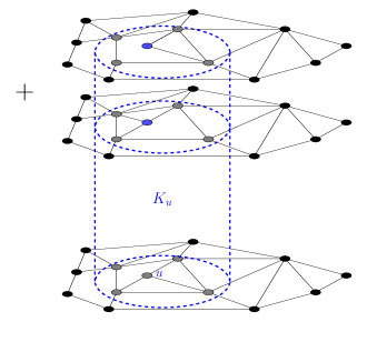
Figure 1: $K_{u}$ is a local unitary gate: it acts locally upon vertex $u$ and its neighbours, and may create superpositions of graphs. Consider global, unitary causal operator, which takes quantum superpositions of entire graphs into quantum superpositions of entire graphs—but in such a way that information propagates from one node to another only if they are neighbours in the graph. In this paper we show that unitary causal operators always decompose as a finite-depth circuit of such local unitary gates.

Plan.

In Sec. II we formalize our state space: superpositions of graphs. In Sec. III we adapt the notion of tensor and partial trace to this state space. In Sec. IV and V we propose and formalize the notions causality and locality in this context, and prove several propositions of general interest. In Sec. VI we prove our main result. Sec. VII provides a summary and perspectives.

II Mathematical preliminaries

The graphs we consider are the usual, finite, undirected, bounded-degree graphs, but with three added twists:

• Edges are between ports of vertices, rather than vertices themselves, so that each vertex can distinguish its different neighbours, via the port that connects to it.

• The vertices are given labels taken in an alphabet, so that they may carry an internal state just like the cells of a Cellular Automaton.

• The labelling function is partial, so that we may express our partial knowledge about part of a graph.

Definition 1 (Graph)

Consider $V$ a countable set of vertices and $\pi$ a finite set of ports. A graph $G$ is given by

• A finite subset $V(G)$ of $V$, whose elements are called vertices.

• A set $E(G)$ of non-intersecting two-elements subsets of $V(G)\times\pi$, whose elements are called edges. In other words an edge $e$ is of the form $\{u\!:\!a,v\!:\!b\}$, and $\forall e,e^{\prime}\in E(G),e\cap e^{\prime}\neq\varnothing\Rightarrow e=e^{\prime}$.

The set of all graphs with vertices in $V$ and ports in $\pi$ is written ${\cal G}_{V,\pi}$. To ease notations, we write $v\in G$ for $v\in V(G)$. We write $\varnothing$ for the empty graph.

Definition 2 (Labelled graph)

A labelled graph is a triple $(G,\sigma)$, also denoted simply $G$ when unambiguous, where $G$ is a graph, and $\sigma$ is a partial function from $V(G)$ to a finite, or countable set $\Sigma$. The set of all labelled graphs with vertices in $V$, ports in $\pi$, and states in $\Sigma$ is written ${\cal G}_{V,\Sigma,\pi}$, or simply ${\cal G}$.

We need a notion of union of graphs, and for this purpose we need a notion of consistency between the operands of the union, so as at to make sure that both graphs “do not disagree”.

Definition 3 (Consistent)

Two graphs $G$ and $H$ in ${\cal G}$ are consistent if and only if:

• over the set $W=(V(G)\cap V(H))$ the partial functions $\sigma_{G}$ and $\sigma_{H}$ agree when they are both defined, meaning that: $\forall u\in W$,

  $$\big{[}u\in\textrm{dom}(\sigma_{G})\wedge u\in\textrm{dom}(\sigma_{H})\Rightarrow\sigma_{G}(u)=\sigma_{H}(u)\big{]}$$

  where $\textrm{dom}(\sigma)$ stands for the domain of $\sigma$.

• the edges adjacent to vertices of $W$ in $G$ and $H$ agree, meaning that: $\forall u\!:\!i\in(W\!:\!\pi)$, $\forall v\!:\!j\in V(G)\!:\!\pi$, $\forall v^{\prime}\!:\!j^{\prime}\in V(H)\!:\!\pi$:

  $$\big{[}\{u\!:\!i,v\!:\!j\}\in E(G)\wedge\{u\!:\!i, v^{\prime}\!:\!j^{\prime}\}\in E(H)$$

  $$\Rightarrow(v=v^{\prime}\wedge j=j^{\prime})\big{]}$$

Definition 4 (Union)

Consider two consistent graphs $G$ and $H$, we define the graph $G\cup H$ to be the graph:

• whose set of vertices $V(G\cup H)$ is $V(G)\cup V(H)$.

• whose partial function $\sigma_{G\cup H}$ has domain $\textrm{dom}(\sigma_{G})\cup\textrm{dom}(\sigma_{H})$ and coincides with $\sigma_{G}$ (resp. $\sigma_{H}$) over $\textrm{dom}(\sigma_{G})$ (resp. $\textrm{dom}(\sigma_{H})$).

We will also need ways of taking subgraphs that induced by the neighbours of a vertex.

Definition 5 (Disks)

Consider $G\in{\cal G}$, and $S\subset V$. We write $D(G)^{r}_{S}$ for the radius $r$ neighbours of $S$ in $G$, i.e. all those vertices which can be reached in $r$ steps, or less, following edges of $G$, starting from a vertex in $S$. This includes $S$. The border vertices of $S$, on the other hand, are the radius $1$ neighbours of $S$ in $G$ which do not lie in $S$.
Now consider $D\subset V$, and $\overline{D}=V\setminus D$. We write $G_{D}$ for the subgraph induced by $D$ and its border vertices, all labellings included except those of the border vertices. We write $\overline{G}_{D}$ for the subgraph induced by $\overline{D}$, all labellings included.
In the special case where $D$ is $D(G)^{r}_{v}$ the set of radius $r$ neighbours of vertex $v$ in $G$, we simply write $G^{r}_{v}$ instead of $G_{D(G)^{r}_{v}}$, and refer to this as a disk. Similarly we write $\overline{G}^{r}_{v}$ instead of $\overline{G}_{D(G)^{r}_{v}}$ and refer to this as the complement of a disk.

Remark 1

Notice that for all $G$ and $D\subset V$, $G=G_{D}\cup\overline{G}_{D}$. Indeed, the decomposition does not miss any out edge between $D$ and $\overline{D}$, as these belong to $G_{D}$.

Having defined the set of labelled graphs, which is infinite but countable, we can readily use it as the canonical basis for a Hilbert space of quantum superpositions of graphs.

Definition 6 (Superpositions of configurations)

We define ${\cal H}_{\cal G}$ be the Hilbert space of labelled graphs, as follows: to each labelled graph $G$ is associated a unit vector $|G\rangle$, such that the family $\left(|G\rangle\right)_{G\in{\cal G}}$ is the canonical orthonormal basis of ${\cal H}_{\cal G}$. A state vector is a unit vector $|\psi\rangle$ in ${\cal H}_{\cal G}$. A state is a trace-one positive operator $\rho$ over ${\cal H}_{\cal G}$. To ease notations, we write $\mathcal{H}$ instead of ${\cal H}_{\cal G}$.

Definition 7 (Vertex preserving)

A linear operator $U:\mathcal{H}\longrightarrow\mathcal{H}$ is said to be vertex preserving if and only if for any graph $G\in{\cal G}$, we have that if $U|G\rangle=\sum_{i}\alpha_{i}|G(i)\rangle$, then for all $i$, $V(G(i))=V(G)$.

III Generalized tensors and traces

In quantum theory, the tensor product is the basic operation used to mathematically represent the joint system of two systems next to one another. Here the systems are lie at vertices of a graph, and so we need to say how they connect to each other. Moreover, the graph itself may be in a superposition, it forms part of the state space. We need to adapt tensor products to this context.

Definition 8 (Generalized Tensors)

We write $|G\rangle\otimes|H\rangle=|G\rangle|H\rangle$ for $|G\cup H\rangle$. The tensor product definition is then bilinearly extended to pairwise consistent superpositions of state vectors in ${\cal H}$.

Comment. Usually a tensor product takes in states $|\psi\rangle^{A}$ and $|\phi\rangle^{B}$ from two non-overlapping systems $A$ and $B$, to produce $|\psi\rangle^{A}|\phi\rangle^{B}$. However, consider a common subsystem $C$ and input states from overlapping systems $AC$ and $BC$. If we demand that they have that the particular form $|\psi\rangle^{A}|\vartheta\rangle^{C}$ and $|\phi\rangle^{B}|\vartheta\rangle^{C}$, then we can naturally extend the tensor product to produce $|\psi\rangle^{A}|\phi\rangle^{B}|\vartheta\rangle^{C}$. This is what the above definition does: the consistency requirement amounts to imposing agreement upon the common subsystem.

Now, if $\rho$ captures the state of an entire system, then $\rho^{r}_{v}$ stands for the state of the neighbours of $v$:

Definition 9 (Generalized partial trace)

Consider $\rho=|G\rangle\langle H|$ over $\mathcal{H}$, with $G,H\in{\cal G}$. Let $D=D(G)^{r}_{v}\cup D(H)^{r}_{v}$. We define its partial trace $\rho^{r}_{v}$ to be

$$|G_{D}\rangle\langle H_{D}|\langle\overline{H}_{D}|\overline{G}_{D}\rangle$$

The definition is linearly extended to any state over $\mathcal{H}$.

Remark 2

From the previous remark, we get that $\textrm{Tr}(\rho)=\textrm{Tr}(\rho^{r}_{v})$.

Comment. On the one hand, the above definition is a straightforward extension of the usual $\textrm{Tr}_{B}(|ij\rangle^{AB}\langle kl|)=|i\rangle^{A}\langle k|\langle j|l\rangle$ formula. On the other hand, the definition intends to let the system $A$ be the disk of radius $r$ centered on $v$—but this a priori is an unclear notion for quantum superpositions of graphs. This issue is solved by addressing the basic case, first, and then extending to superpositions.

IV Causality

A fundamental symmetry of physics is causality, meaning that information propagates at a bounded speed. In discrete space and time, this means that in order to know the next state and connectivity of a vertex $v$, we only need to know that of its neighbours at the previous time step:

Definition 10 (Causality)

A linear operator $U:\mathcal{H}\longrightarrow\mathcal{H}$ is said to be causal if and only if for all $m\geq 0$ there exists $n\geq 0$ such that for any state $\rho$ over $\mathcal{H}$, and for any $v\in V$, we have

$$(U\rho U^{\dagger})^{m}_{v}=(U\rho^{n}_{v}U^{\dagger})^{m}_{v}.$$ (1)

Comment. The above is a direct translation of causality, as expressed with our generalized partial trace. Notice how, in the case of basic states, this definition of causality specializes into the usual notion of causality as in classical Causal Graph Dynamics ArrighiCayley ; ArrighiRC . Notice also how, in the case of fixed graphs whose nodes are labelled by quantum states, this definition of causality again specializes into that used for Quantum Cellular Automata ArrighiUCAUSAL ; ArrighiJCSS . What happens in the grey zone of quantum superpositions of graphs may seem a little wilder, but in the end it is just the linear extension of these notions.

The following proposition will turn out useful.

Proposition 1 (Tensorial extension)

Given a causal unitary operator $U$ over ${\cal H}$,

$$U^{\prime\prime}:{\cal H}\otimes{\cal H} \longrightarrow{\cal H}\otimes{\cal H}$$

$$U^{\prime\prime} =U\otimes I$$

is causal. Here, ${\cal H}\otimes{\cal H}\equiv{\cal H}_{{\cal G}^{2}}\equiv{\cal H}_{{\cal G}\uplus{\cal G}}$.

Proof.

$$(U^{\prime\prime}\rho^{\prime}U^{\prime\prime\dagger})^{m}_{v}= (U^{\prime\prime}(\sum_{i}\rho(i)\otimes\tau(i))U^{\prime\prime\dagger})^{m}_{v}$$

$$= \sum_{i}(U\rho(i)U^{\dagger})^{m}_{v}\otimes\tau(i)^{m}_{v}$$

$$= \sum_{i}(U\rho(i)^{n}_{v}U^{\dagger})^{m}_{v}\otimes(\tau(i)^{n}_{v})^{m}_{v}$$

$$= (U^{\prime\prime}\sum_{i}(\rho(i)\otimes\tau(i))^{n}_{v})U^{\prime\prime\dagger})^{m}_{v}$$

$$= (U^{\prime\prime}\rho^{\prime n}_{v}U^{\prime\prime\dagger})^{m}_{v}$$

$\Box$

V Locality

Causal operators change the entire graph in one go. The word causal there refers to the fact that information does not propagate too fast. Local operations, on the other hand, act just in one bounded region of the graph, leaving the rest unchanged:

Definition 11 (Localization)

A linear operator $A:\mathcal{H}\longrightarrow\mathcal{H}$ is said to be $r$-localized upon $v\in V$ if and only if for any $G,H\in{\cal G}$, we have that

$$\langle H|A|G\rangle =\langle H_{D}|A|G_{D}\rangle\langle\overline{H}_{D}|\overline{G}_{D}\rangle$$ (2)

with $D=D(G)^{r}_{v}\cup D(H)^{r}_{v}$.

In other words, $A$ only changes $v$ and its neighbours, and only requires knowledge of $v$ and its neighbours to do that. Thought of as a measurement, $A$ is only sensitive to changes in $v$ and its neighbours:

Proposition 2 (Dual localization)

Let $A$ be an $r$-local linear operator, upon a vertex $v$. This is equivalent to saying that for any two states $\rho,\rho^{\prime}$ over $\mathcal{H}$, we have that $\rho^{r}_{v}=(\rho^{\prime})^{r}_{v}$ entails that $\textrm{Tr}(A\rho)=\textrm{Tr}(A\rho^{\prime})$.

$[\Rightarrow]$. Suppose that $A$ is $r$-localized upon a vertex $v\in V$. For any $\rho=|G\rangle\langle H|$ let $D=D(G)^{r}_{v}\cup D(H)^{r}_{v}$. We have:

$$\textrm{Tr}\left(A\rho\right) =\langle H|A|G\rangle$$

$$=\langle H_{D}|A|G_{D}\rangle\langle\overline{H}_{D}|\overline{G}_{D}\rangle$$

$$=\textrm{Tr}\left(A|G_{D}\rangle\langle H_{D}|\langle\overline{H}_{D}|\overline{G}_{D}\rangle\right)$$

$$=\textrm{Tr}\left(A\rho^{r}_{v}\right)$$

Assuming $\rho^{r}_{v}={\rho^{\prime}}^{r}_{v}$ yields $\textrm{Tr}\left(A\rho\right)=\textrm{Tr}\left(A\rho^{r}_{v}\right)=\textrm{Tr}\left(A\rho^{\prime r}_{v}\right)=\textrm{Tr}\left(A\rho^{\prime}\right)$.

$[\Leftarrow]$. Let us assume that $A$ is dually $r$-local around $v$. For any $\rho=|G\rangle\langle H|$ Let $D=D(G)^{r}_{v}\cup D(H)^{r}_{v}$. We have:

$$\langle H|A|G\rangle =\textrm{Tr}\left(A\rho\right)$$

$$=\textrm{Tr}\left(A\rho^{r}_{v}\right)\;\textrm{using dual localization.}$$

$$=\textrm{Tr}\left(A|G_{D}\rangle\langle H_{D}|\langle\overline{H}_{D}|\overline{G}_{D}\rangle\right)$$

$$=\langle H_{D}|A|G_{D}\rangle\langle\overline{H}_{D}|\overline{G}_{D}\rangle$$

Now that we have a notion of locality, we can rephrase that of causality in the Heisenberg picture, which is the more traditional one in algebraic quantum field theory for instance.

Proposition 3 (Dual causality)

Let $U$ be a causal linear operator. This is equivalent to saying that for every operator $A$ $m$-localized upon vertex $v$, then $U^{\dagger}AU$ is $n$-localized upon vertex $v$.

Proof. $[\Rightarrow]$. Suppose causality and let $A$ be an operator $m$-localized upon vertex $v$. Let $n$ be that from Def. 10. For every pair of states $\rho$ and $\rho^{\prime}$ such that $\rho^{n}_{v}={\rho^{\prime}}^{n}_{v}$, we have $\left(U\rho U^{\dagger}\right)^{m}_{v}=\left(U\rho^{\prime}U^{\dagger}\right)^{m}_{v}$ and hence $\textrm{Tr}\left(AU\rho U^{\dagger}\right)=\textrm{Tr}\left(AU\rho^{\prime}U^{\dagger}\right)$. We thus get $\textrm{Tr}\left(U^{\dagger}AU\rho\right)=\textrm{Tr}\left(U^{\dagger}AU\rho^{\prime}\right)$. Since this equality holds for every $\rho$ and $\rho^{\prime}$ such that $\rho^{n}_{v}={\rho^{\prime}}^{n}_{v}$, we have that $U^{\dagger}AU$ is $n$-localized.
$[\Leftarrow]$. Suppose dual causality and $\rho^{n}_{v}={\rho^{\prime}}^{n}_{v}$. Then, for every operator $B$ $n$-localized upon $v$, $\textrm{Tr}\left(B\rho\right)=\textrm{Tr}\left(B\rho^{\prime}\right)$, and so for every operator $A$ $m$-localized upon vertex $v$, we get: $\textrm{Tr}\left(AU\rho U^{\dagger}\right)=\textrm{Tr}\left(U^{\dagger}AU\rho\right)=\textrm{Tr}\left(U^{\dagger}AU\rho^{\prime}\right)=\textrm{Tr}\left(AU\rho^{\prime}U^{\dagger}\right).$ This entails $\left(U\rho U^{\dagger}\right)^{m}_{v}=\left(U\rho^{\prime}U^{\dagger}\right)^{m}_{v}$. $\Box$

VI Representation theorem

The goal of this section is to achieve a representation of causal operators as a bounded-depth circuit of local unitary operators. The idea of this construction is to proceed by local updates. We will construct local operators $K_{u}$ updating only the neighbourhood of a vertex $u$. All these $K_{u}$ will be local unitary operators and will commute with each other. To do so, we generalize the construction presented in ArrighiBRCGD : the local update $K_{u}$ consists in applying the causal operator $U$, “putting aside” vertex $u$ from the graph, and applying the inverse operator $U^{\dagger}$.

First, we construct an appropriate state space, allowing us to ‘mark’ vertices in order to “put them aside” as computed.

Definition 12 (Marked graphs and space)

Given a set of graphs ${\cal G}={\cal G}_{V,\Sigma,\pi}$, consider the set of graphs ${\cal G}_{V,\Sigma^{\prime},\pi^{\prime}}$ with $\Sigma^{\prime}=\Sigma\times\{0,1\}$ and $\pi^{\prime}=\pi\times\{0,1\}$. We define the set of marked graphs ${\cal G}^{\prime}$, to be the subset of ${\cal G}_{V,\Sigma^{\prime},\pi^{\prime}}$ such that for all graph $G\in{\cal G}^{\prime}$, for all vertex $u\in G$ with $\sigma_{G}(u)=(x,a)$ and $\{u:(i,b),v:(j,c)\}\in G$, we have $a=c$. We denote by ${\cal H}^{\prime}$ the state space whose basis vectors are the marked graphs ${\cal G}^{\prime}$. Given a graph $G\in\mathcal{G}$, it is naturally identified with the same graph in ${\cal G}^{\prime}$ with all marks set to $0$.

The following definition introduces our marking mechanism.

Definition 13 (Mark operator)

Given a set of labels $\Sigma^{\prime}=\Sigma\times\{0,1\}$ and a set of ports $\pi^{\prime}=\pi\times\{0,1\}$, we define the marking operation $\mu(.)$ over labels and ports as toggling the bit in the second component:

• $\forall(x,a)\in\Sigma^{\prime},\mu(x,a)=(x,1-a)$

• $\forall(i,a)\in\pi^{\prime},\mu(i,a)=(i,1-a)$

Then, we define the mark operation $\mu_{u}$ over marked graphs, as attempting to mark the label of vertex $u$ and its opposite ports, if this will not create conflicts between ports. More formally, given a graph $G$ in ${\cal G}^{\prime}$, we define the mark operation, $\mu_{u}:{\cal G}^{\prime}\rightarrow{\cal G}^{\prime}$ as follows:

• if $\exists v,w\in G,i,j\in\pi^{\prime}$ such that $\{u\!:\!i,v\!:\!j\}\in G$ and $\{v\!:\!\mu(j),w\!:\!k\}\in G$ then $\mu_{u}G=G$

• else

  • $\sigma_{\mu_{u}G}(u)=\mu(\sigma_{G}(u))$

  • For all $i,j\in\pi^{\prime}$, $\{u\!:\!\mu(i),u\!:\!\mu(j)\}\in\mu_{u}G$ if and only if $\{u\!:\!i,u\!:\!j\}\in G$.

  • For all $v\in G$ with $v\neq u$ and $i,j\in\pi^{\prime}$, $\{u\!:\!i,v\!:\!\mu(j)\}\in\mu_{u}G$ if and only if $\{u\!:\!i,v\!:\!j\}\in G$.

  with the rest of the graph $G$ left unchanged.

Finally, $\mu_{u}$ is linearly extended to become a unitary operator over ${\cal H}^{\prime}$. Moreover each $\mu_{u}$ is $1$-localized and commutes with $\mu_{v}$ for all $v$.

Soundness. As $\mu_{u}$ specifies a bijection over the set of graphs ${\cal G}^{\prime}$, its linear extension to ${\cal H}^{\prime}$ is unitary. Moreover, $\mu_{u}$ only changes the label of vertex $u$ and the ports of its adjacent edges, but it does so conditionally upon the edges of the neighbours, which makes it $1$-localized. Finally, when $u\neq v$, then $\mu_{u}$ and $\mu_{v}$ either both act independently upon disjoint labels and ports, or they are both the identity—hence they commute.

It turns out that any causal operator admits an extension that is compatible with these marks.

Proposition 4 (Marked extension)

Given a vertex-preserving causal unitary operator $U$ over ${\cal H}$, there exists a vertex-preserving causal unitary operator $U^{\prime}$ over ${\cal H}^{\prime}$ such that:

$$\forall G\in{\cal G}_{V,\Sigma\times\{0\},\pi\times\{0\}}, \quad U^{\prime}|G\rangle=U|G\rangle$$

$$\forall G\in{\cal G}_{V,\Sigma\times\{1\},\pi\times\{1\}}, \quad U^{\prime}|G\rangle=|G\rangle$$

Proof. Consider

$$U^{\prime\prime}:{\cal H}\otimes{\cal H} \longrightarrow{\cal H}\otimes{\cal H}$$

$$U^{\prime\prime} =U\otimes I$$

instead—which is causal by Proposition 1. Notice that ${\cal H}\otimes{\cal H}\equiv{\cal H}_{{\cal G}^{2}}$. We now consider

$$\varphi:{\cal G}^{\prime} \longrightarrow{\cal G}^{2}$$

$$G \mapsto(\overline{G}_{M},\mu_{M}G_{M})$$

with $M$ the marked vertices of $G$. The function $\varphi$ is injective since if $\varphi(G^{\prime})=(G,H)$ then we can recover $G^{\prime}$ as $G\cup(\mu_{M}H)$ with $M=V(H)\backslash V(G)$. Let $S=\varphi(\cal{G}^{\prime})$ be the image of $\varphi$.

Notice that, if $(X,H)\in S$ and $Y\in{\cal G}$ is such that $V(X)=V(Y)$, then $(Y,H)\in S$. Indeed, if $(X,H)$ has antecedent $X^{\prime}=X\cup(\mu_{M}H)$ then the union $Y^{\prime}=Y\cup(\mu_{M}H)$ is well-defined as $\mu_{M}H$ does not specify any internal state or connectivity in $\pi\times\{0\}$ over $V(H)\cap V(X)=V(H)\cap V(Y)$. Moreover, $\varphi(Y^{\prime})=(Y,H)$ because since $V(X)=V(Y)$, $\overline{Y^{\prime}}_{M}=Y$ and $\mu_{M}Y^{\prime}_{M}=\mu_{M}X^{\prime}_{M}=H$.

The subspace ${\cal H}_{S}$ is stable under $U^{\prime\prime}$. Indeed, consider $(G,H)\in S$

$$U^{\prime\prime}(|G\rangle\otimes|H\rangle) =(U|G\rangle)\otimes|H\rangle$$

$$=\sum\alpha_{i}|G(i)\rangle\otimes|H\rangle$$

and notice that for all $i$, $(G(i),H)\in S$ because $V(G(i))=V(G)$.

Next, take $U^{\prime}$ to be the restriction of $U^{\prime\prime}$ to $S$:

$$U^{\prime}:{\cal H}^{\prime} \longrightarrow{\cal H}^{\prime}$$

$$|G^{\prime}\rangle \mapsto(\varphi^{\dagger}\circ U^{\prime\prime}\circ\varphi)|G^{\prime}\rangle$$

where $\varphi$ is linearly extended to be a unitary operator from ${\cal H}^{\prime}$ to ${\cal H}_{S}$. We have the two requested properties. Indeed, $\forall G\in{\cal G}_{V,\Sigma\times\{0\},\pi\times\{0\}}$,

$$U^{\prime}|G\rangle =\varphi^{\dagger}(U\otimes I)(|G\rangle\otimes|\varnothing\rangle)$$

$$=\varphi^{\dagger}(U|G\rangle\otimes|\varnothing\rangle)$$

$$=U|G\rangle$$

and $\forall G\in{\cal G}_{V,\Sigma\times\{1\},\pi\times\{1\}}$,

$$U^{\prime}|G\rangle =\varphi^{\dagger}(U\otimes I)(|\varnothing\rangle\otimes|\mu_{V(G)}\,G\rangle)$$

$$=\varphi^{\dagger}(|\varnothing\rangle\otimes|\mu_{V(G)}\,G\rangle)$$

$$=|G\rangle$$

Causality and vertex preservation are inherited from $U^{\prime\prime}$.   $\Box$

The following theorem is our main contribution:

Theorem 1 (Structure theorem)

Let $U$ be a vertex-preserving unitary causal operator over space ${\cal H}$. Then, in ${\cal H}^{\prime}$ there exists $(K_{u})$ such that for all $|\psi\rangle$:

$$U|\psi\rangle=(\prod_{u\in V}\mu_{u})\,(\prod_{u\in V}K_{u})\,|\psi\rangle$$

where $(K_{u})$ is a collection of commuting unitary $n$-localized operators.

Proof. Let us consider a causal operator $U$ over ${\cal H}$. We define $K_{u}$ as $U^{\prime\dagger}\mu_{u}U^{\prime}$, where $U^{\prime}$ is a marked extension of $U$. Using the causality of $U^{\prime}$ and the dual causality property, we have that $K_{u}$ is a $n$-localized operator. Moreover, it is easy to see that for two distinct vertices $u$ and $v$:

$$K_{u}K_{v} =U^{\prime\dagger}\mu_{u}U^{\prime}U^{\prime\dagger}\mu_{v}U^{\prime}$$

$$=U^{\prime\dagger}\mu_{u}\mu_{v}U^{\prime}$$

$$=U^{\prime\dagger}\mu_{v}\mu_{u}U^{\prime} \mu_{\bullet}$$ using commutativity of

$$=U^{\prime\dagger}\mu_{v}U^{\prime}U^{\prime\dagger}\mu_{u}U^{\prime}$$

$$=K_{v}K_{u}$$

Hence, $(K_{u})$ is a collection of localized commutating operators, thus the product $(\prod_{u}K_{u})$ is well defined.
Now let us unfold the product $(\prod_{u}K_{u})$ and apply it to $|G\rangle$, with $V(G)=\{u_{1},\ldots,u_{k}\}$:

$$K_{u_{1}}K_{u_{2}}\cdots K_{u_{k}}|G\rangle =U^{\prime\dagger}\mu_{u_{1}}U^{\prime}U^{\prime\dagger}\mu_{u_{2}}U^{\prime}\cdots U^{\prime\dagger}\mu_{u_{k}}U^{\prime}|G\rangle$$

$$=U^{\prime\dagger}\mu_{u_{1}}\mu_{u_{2}}\cdots\mu_{u_{k}}U^{\prime}|G\rangle$$

$$=U^{\prime\dagger}\mu_{u_{1}}\mu_{u_{2}}\cdots\mu_{u_{k}}U|G\rangle$$

by construction of $$U^{\prime}$$

$$=\mu_{u_{1}}\mu_{u_{2}}\cdots\mu_{u_{k}}U|G\rangle$$

Hence, applying $(\prod_{u}\mu_{u})(\prod_{u}K_{u})$ results in applying $(\prod_{u}\mu_{u})^{2}U$ which is just $U$.

The general implications of this Theorem are discussed in Secs I and VII. Mathematically speaking, the following two corollaries immediately follow.

Corollary 1 (Inverse of unitary causal is causal)

Let $U$ be a vertex-preserving unitary causal operator over space ${\cal H}$. Then, $U^{\dagger}$ is also causal.

Proof outline. The hypotheses imply localizability. The obtained circuit can then be reversed so as to implement $U^{\dagger}$. It follows that $U^{\dagger}$ is localizable, and hence causal.

Corollary 2 (Unitary 1-causal is causal)

An operator $U$ over $\mathcal{H}$ is said to be 1-causal if and only if it is vertex preserving and there exists $n\geq 0$ such that for any state $\rho$ over $\mathcal{H}$, and for any $v\in V$, we have

$$(U\rho U^{\dagger})^{1}_{v}=(U\rho^{n}_{v}U^{\dagger})^{1}_{v}.$$ (3)

Let $U$ be a vertex-preserving unitary $1$-causal operator over space ${\cal H}$. Then, $U$ is causal.

Proof outline. By inspection of the proofs above, it suffices to be $1$-causal in order to be localizable. But then localizability implies causality.

Notice that we could have followed the same reasoning for $0$-causality if the mark operator could have been made $0$-local, but avoiding port conflicts forces it to be $1$-local. Ultimately the demand to avoid port conflict is to ensure that the graphs remain bounded degree at all times. This in turn is just a choice: with unbounded degree graphs QuantumGraphity1 ; QuantumGraphity2 this question would not arise, and $0$-causality would imply causality. But then these graphs would be much harder to interpret geometrically, as dual to pseudo-manifolds ArrighiSURFACES or spin networks.

VII Summary and future work

We took as our state space the Hilbert space of quantum superpositions of finite, undirected, bounded-degree, labelled graphs. We adapted the notions of tensor product, partial trace, causality and locality to this context, mainly through the idea that they should coincide with their traditional counterparts whenever the graph is not in a superposition—and extending from there by linearity. We recovered a number of reassuring results, such as the duality between causality phrased in the Shrödinger picture (i.e. $(U\rho U^{\dagger})^{m}_{v}=(U\rho^{n}_{v}U^{\dagger})^{m}_{v}$) and that phrased in the Heisenberg picture (i.e. if $A$ is localized, so is $U^{\dagger}AU$), and a similar duality for localizabity.
Mainly, we showed that any vertex-preserving, global unitary causal operator $U$, decomposes into a finite-depth circuit of local unitary gates $\mu$ and $K$:

$$U|\psi\rangle=(\prod\mu_{u})(\prod K_{u})|\psi\rangle$$

thereby making the model constructive and parametrizable. Here $\mu$ is just a fixed, marking operator: only the $K_{u}$’s depend upon $U$. These commute: $[K_{u},K_{v}]=0$. Hence the first product, which is the relevant one, can be spectrally decomposed.

Here are two items for future work:

• The structure theorem was proven under the assumption that the global evolution is vertex-preserving. We wish to understand whether this condition can be relaxed. For instance, even in the model as it stands, we could attach to each vertex some ‘reservoir’ of vertices, structured as an infinite binary tree. The quantum causal graph dynamics would then be able to ‘create’ vertices by pulling them out of the reservoir, and to ‘destroy’ them by pushing them back in. We plan to investigate this question in the near future.

• Our framework is canonical, in the sense that it relies upon a distinguished discrete-time evolution. It cannot, therefore, be manifestly covariant in the sense of general relativity—but the perhaps covariance of some instances could be proven, e.g. in the style of arrighi2014discrete .

VIII Quantum gravity landscape

Digital Physics, of which a prominent actor is tHooftCA , seeks to recover modern theoretical physics concepts as emergent from a Reversible Cellular Automata. The above-presented Quantum Causal Graph Dynamics clearly arises as a two-fold extension of Reversible Cellular Automata — an extension to dynamical graphs on the one hand, and to quantum theory on the other hand. In this sense it shares common origins with the digital physics program, but it also departs from it: both quantum dynamics and geometrodynamics WheelerGeo are seen as fundamental features that one needs to put in.

Quantum Graphity QuantumGraphity1 ; QuantumGraphity2 discretizes ‘pre-geometrical space’ as a complete graph, with qubits on each edge telling whether its end vertices are neighbours or not. These qubits are then made to evolve according to a nearest-neighbours Hamiltonian. Quantum Graphity thus does not place space and time on a equal footing, as one is discrete and the other continuous. It follows that, strictly speaking, after any finite period of time, information has propagated everywhere: causality is approximate, in the sense of a Lieb-Robinson bound EisertSupersonic . Quantum Causal Graph Dynamics can be seen as a theory of discrete-time quantum graphity.

Quantum Causal Histories FotiniQCH , on the other hand, does look at global unitary evolutions between two spacelike surfaces—but the fact that it decomposes into local unitary gates is directly assumed in this approach. The local unitary gates are also located at each vertex, and act upon the quantum information circulating upon the edges—but have no influence upon the graph itself. The causal set is given, and in no superposition.

Emergence of almost-flat space. In quantum graphity, the underlying graph is complete, which makes its geometrical interpretation very difficult. Some bounded-degree graphs, on the other hand, can be understood as pseudo-manifolds Lickorish ; GrasselliGems ; ArrighiSURFACES . Thus a more long-term aim is to retake this inspiring program of emergence of almost-flat space QuantumGraphity1 ; QuantumGraphity2 but in this discrete-space discrete-time bounded-degree-graphs formalism. Alternatively and interestingly, almost-flatness can also be seen as an emergent property of certain probability distribution over graphs TrugenbergerEmergent1 ; TrugenbergerEmergent2 , e.g. via clustering KrioukovEmergent .

Loop Quantum Gravity RovelliLQG , one of the main contenders for a theory of Quantum Gravity, also provides means of computing the transition amplitude of one space-like graph evolving into another. Yet its relationship with the above-presented Quantum Causal Graph Dymanics is unclear to us at this stage. Indeed, in Loop Quantum Gravity, the transition amplitude between the two spin networks, that make up the past and future boundaries of a spacetime region, is provided in a path-integral form by summing over the possible spin foams that could relate them. It follows that: the ‘time taken for the transition to happen’ is also summed over; that the evolution is not guaranteed to be unitary; and that far-away vertices of the spin networks are allowed to signal to some extent. Actually, spin networks are not directly interpretable as discretized space-like surfaces in Loop Quantum Gravity: only coherent superpositions of them correspond to piecewise-linear manifolds in a one-to-one manner. These are some of the key differences that stand in the way of bridging this gap, which we believe would be a fruitful program.

Causal Dynamical Triangulations LollCDT lets some of these difficulites vanish. It lifts the ambiguity of spin networks and directly works with glued equilateral tetrahedras. It works out the transition amplitude between two discretized space-like space surfaces that are separated by a given proper time. It does so in a path-integral form, by summing over the possible successive surfaces that could relate them — but these successive surfaces are themselves related by local ’moves’. Still it is unclear whether this induces a unitary evolution operator over discretized space-like space surfaces. Moreover here again and far-away parts of the triangulation are allowed to signal to some extent.

Summarizing, quantum causal graph dynamics provide a mathematical framework for discrete-time quantum gravity models that exhibit both strict causality and strict unitary. To the best of our knowledge, to this day none of the main quantum gravity models gathers all of these features at once. Several of them are not so far. Gathering the reminding features would make the model fall within the scope of the structure theorem of this paper, and therefore decompose into local unitary scattering matrices $K$. This would pave the way towards quantum simulating Quantum Gravity.

References

- (1) Jan Ambjørn, Jerzy Jurkiewicz, and Renate Loll. Emergence of a 4d world from causal quantum gravity. Physical review letters, 93(13):131301, 2004.
- (2) P. Arrighi and G. Dowek. Causal graph dynamics. In Proceedings of ICALP 2012, Warwick, July 2012, LNCS, volume 7392, pages 54–66, 2012.
- (3) P. Arrighi, R. Fargetton, V. Nesme, and E. Thierry. Applying causality principles to the axiomatization of Probabilistic Cellular Automata. In Proceedings of CiE 2011, Sofia, June 2011, LNCS, volume 6735, pages 1–10, 2011.
- (4) P. Arrighi and S. Martiel. Generalized Cayley graphs and cellular automata over them. In Proceedings of GCM 2012, Bremen, September 2012. Pre-print arXiv:1212.0027, pages 129–143, 2012.
- (5) P. Arrighi, S. Martiel, and Z. Wang. Causal dynamics over Discrete Surfaces. In Proceedings of DCM’13, Buenos Aires, August 2013, EPTCS, 2013.
- (6) P. Arrighi, V. Nesme, and R. Werner. Unitarity plus causality implies localizability. J. of Computer and Systems Sciences, 77:372–378, 2010. QIP 2010 (long talk).
- (7) P. Arrighi, V. Nesme, and R. Werner. Unitarity plus causality implies localizability (full version). Journal of Computer and System Sciences, 77(2):372–378, 2011.
- (8) P. Arrighi, V. Nesme, and R. F. Werner. Quantum cellular automata over finite, unbounded configurations. In Proceedings of LATA, Lecture Notes in Computer Science, volume 5196, pages 64–75. Springer, 2008.
- (9) P. Arrighi, V. Nesme, and R. F. Werner. One-dimensional quantum cellular automata. IJUC, 7(4):223–244, 2011.
- (10) Pablo Arrighi, Stefano Facchini, and Marcelo Forets. Discrete lorentz covariance for quantum walks and quantum cellular automata. New Journal of Physics, 16(9):093007, 2014.
- (11) Pablo Arrighi, Simon Martiel, and Simon Perdrix. Block representation of reversible causal graph dynamics. In Proceedings of FCT 2015, Gdansk, Poland, August 2015, pages 351–363. Springer, 2015.
- (12) Pablo Arrighi, Simon Martiel, and Simon Perdrix. Reversible causal graph dynamics. In Proceedings of International Conference on Reversible Computation, RC 2016, Bologna, Italy, July 2016, pages 73–88. Springer, 2016.
- (13) D. Beckman, D. Gottesman, M. A. Nielsen, and J. Preskill. Causal and localizable quantum operations. Phys. Rev. A., 64(052309), 2001.
- (14) J. O. Durand-Lose. Representing reversible cellular automata with reversible block cellular automata. Discrete Mathematics and Theoretical Computer Science, 145:154, 2001.
- (15) Jens Eisert and David Gross. Supersonic quantum communication. Physical review letters, 102(24):240501, 2009.
- (16) Luigi Grasselli. Crystallizations and other manifold representations. Disertaciones Matemáticas del Seminario de Matemáticas Fundamentales, 1:1–17, 1987.
- (17) A. Hamma, F. Markopoulou, S. Lloyd, F. Caravelli, S. Severini, K. Markstrom, C. Brouder, Â. Mestre, F.P. JAD, A. Burinskii, et al. A quantum Bose-Hubbard model with evolving graph as toy model for emergent spacetime. Arxiv preprint arXiv:0911.5075, 2009.
- (18) G. A. Hedlund. Endomorphisms and automorphisms of the shift dynamical system. Math. Systems Theory, 3:320–375, 1969.
- (19) J. Henson. Comparing causality principles. Studies In History and Philosophy of Science Part B: Studies In History and Philosophy of Modern Physics, 36(3):519–543, 2005.
- (20) J. Kari. Representation of reversible cellular automata with block permutations. Theory of Computing Systems, 29(1):47–61, 1996.
- (21) J. Kari. On the circuit depth of structurally reversible cellular automata. Fundamenta Informaticae, 38(1-2):93–107, 1999.
- (22) T. Konopka, F. Markopoulou, and L. Smolin. Quantum graphity. Arxiv preprint hep-th/0611197, 2006.
- (23) Dmitri Krioukov. Clustering implies geometry in networks. Phys. Rev. Lett., 116:208302, May 2016.
- (24) WB Raymond Lickorish. Simplicial moves on complexes and manifolds. Geometry and Topology Monographs, 2(299-320):314, 1999.
- (25) Fotini Markopoulou. Quantum causal histories. Classical and Quantum Gravity, 17(10):2059, 2000.
- (26) Carlo Rovelli. Simple model for quantum general relativity from loop quantum gravity. In Journal of Physics: Conference Series, volume 314, page 012006. IOP Publishing, 2011.
- (27) B. Schumacher and R. Werner. Reversible quantum cellular automata. arXiv pre-print quant-ph/0405174, 2004.
- (28) B. Schumacher and M. D. Westmoreland. Locality and information transfer in quantum operations. Quantum Information Processing, 4(1):13–34, 2005.
- (29) Gerard t’Hooft. The Cellular Automaton Interpretation of Quantum Mechanics, volume 185 of Fundamental Theories of Physics. Springer, 2016.
- (30) Carlo A Trugenberger. Combinatorial quantum gravity. arXiv preprint arXiv:1610.05934, 2016.
- (31) Carlo A Trugenberger. Random holographic “large worlds” with emergent dimensions. Physical Review E, 94(5):052305, 2016.
- (32) John Archibald Wheeler. Geometrodynamics. 1962.