X-Raying the Dark Side of Venus - Scatter from Venus Magnetotail?

Abstract

This work analyzes the X-ray, EUV and UV emission apparently coming from the Earth-facing (dark) side of Venus as observed with Hinode/XRT and SDO/AIA during a transit across the solar disk occurred in 2012. We have measured significant X-Ray, EUV and UV flux from Venus’ dark side. As a check we have also analyzed a Mercury transit across the solar disk, observed with Hinode/XRT in 2006. We have used the latest version of the Hinode/XRT Point Spread Function (PSF) to deconvolve Venus and Mercury X-ray images, in order to remove possible instrumental scattering. Even after deconvolution, the flux from Venus’  shadow remains significant while in the case of Mercury it becomes negligible. Since stray-light contamination affects the XRT Ti-poly filter data from the Venus transit in 2012, we performed the same analysis with XRT Al-mesh filter data, which is not affected by the light leak. Even the Al-mesh filter data show residual flux.
We have also found significant EUV (304 Å, 193 Å, 335 Å) and UV (1700 Å) flux in Venus’ shadow, as measured with SDO/AIA. The EUV emission from Venus’ dark side is reduced when appropriate deconvolution methods are applied; the emission remains significant, however.
The light curves of the average flux of the shadow in the X-ray, EUV, and UV bands appear different as Venus crosses the solar disk, but in any of them the flux is, at any time, approximately proportional to the average flux in a ring surrounding Venus, and therefore proportional to the average flux of the solar regions around Venus’ obscuring disk line of sight. The proportionality factor depends on the band.
This phenomenon has no clear origin; we suggest it may be due to scatter occurring in the very long magnetotail of Venus.

1 Introduction

Transits of Mercury and Venus across the solar disk are well-observed celestial phenomena. Recently, the transit of Mercury observed with Hinode/X-Ray Telescope (XRT; Golub et al. 2007) has been used by Weber et al. (2007) to test the sharpness of the instrument Point Spread Function (PSF). Reale et al. (2015) used Hinode/XRT observations of a Venus transit to measure the size of Venus in the X-ray band thus inferring the extension and optical thickness of Venus’ atmosphere. The methods and implications of the latter work reach into planetary physics and hint at similar methods to be potentially used, in the future, for exoplanets.
In this work we analyze the same set of observations to explore the residual X-ray emission observed in Venus’ shadow and find, with the help of an updated version of the Hinode/XRT PSF, that this emission is not due to instrumental scattering and may have an origin more directly related to Venus. Previous observations with Chandra in 2001 and then in 2006/2007 confirmed the X-ray emission from the sunlit side of the Venus (Dennerl 2002 and Dennerl 2008).
In Section 2 we present the observations of Mercury and Venus with a brief summary of the satellites and their instruments; in Section 3 we measure the residual flux in the shadow of Mercury in X-ray and of Venus in X-Ray, EUV and UV bands, and its evolution as Venus crosses the solar disk. In Section 4 we deconvolve X-ray images using the updated PSF and different codes, and again explore similarities and differences among the various observations; in Section 5 we describe the XRT straylight contamination and present our results taken with the Al-mesh filter. In Section 6 we show similar results obtained in EUV and UV bands. Section 7 contains our discussion and the conclusions.

2 Observation: Transit of Mercury and Venus

On 2006 Nov 08, Mercury passed across the solar disk. Its transit lasted for almost five hours and was observed with Hinode/XRT in the X-ray band; Fig. 1 shows a selected image of this phenomenon.
A Venus transit was observed with Hinode/XRT in 2012 while it was crossing the northern hemisphere of the Sun; the transit lasted over six hours. On the 5th of June 2012, the Venus transit began at 22:09 UTC and finished on June 6th at 04:49 UTC. The Venus transit was also observed with the Solar Dynamics Observatory/Atmospheric Imaging Assembly (SDO/AIA) (Pesnell et al., 2012) in the Ultraviolet (UV) and Extreme Ultraviolet (EUV) bands. Fig. 1 shows an image taken during this transit.
In the following we briefly discuss the satellites and the instruments which took the data used in this work.

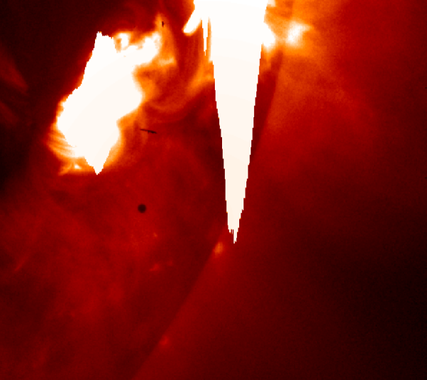
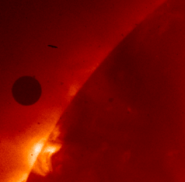
Figure 1: Left: Mercury transit across the Sun observed with Hinode/XRT in the X-Ray band.
(Time of observation, 2006-11-08 23:51:04.571).
Right: Venus (black circle) approaching the Sun, observed with Hinode/XRT in the X-Ray band.
(Time of observation 2012-06-05 21:57:39.893).

2.1 Hinode/XRT

The Hinode satellite (formerly Solar-B) of the Japan Aerospace Exploration Agency’s Institute of Space and Astronautical Science (ISAS/JAXA) was successfully launched in September 2006. There are three instruments onboard: the Solar Optical Telescope (SOT), the EUV Imaging Spectrometer (EIS), and the X-Ray Telescope (XRT). We used only data from XRT.
XRT is a high-resolution grazing-incidence telescope with a modified Wolter-I telescope design that uses grazing incidence optics with an angular resolution consistent with 1.0286 arcsec per pixel at the CCD (Golub et al., 2007).
An improved version of the Hinode/XRT PSF has been derived by P. R. Jibben of the XRT instrument team. The Model PSF has 99% of the encircled energy within a 100 arcsec diameter with the remaining 1% scattered beyond. The PSF model at 0.56 keV is:

$$PSF=\begin{cases}a\frac{exp(-\frac{r^{2}}{\sigma^{2}})}{\gamma^{2}+r^{2}},&\text{if $r\leq 3.4176$};\\ \frac{0.03}{r},&\text{if $3.4176\leq r\leq 5$};\\ \frac{0.15}{r^{2}},&\text{if $5\leq r\leq 11.1$};\\ \frac{(11.1)^{2}\times 0.15}{r^{4}},&\text{if $r\geq 11.1$};\par\end{cases}$$

Where r = radial distance in arc seconds, a = 1.31946, $\sigma=2.19256$ and $\gamma=1.24891$.

This PSF is planned for distribution in the XRT branch of SolarSoft (Freeland & Bentley, 2000) (Bentley & Freeland, 1998).

2.2 SDO/AIA

The Solar Dynamics Observatory (SDO) was launched on February 11, 2010. The spacecraft includes three instruments: the Extreme Ultraviolet Variability Experiment (EVE), the Helioseismic and Magnetic Imager (HMI), and the Atmospheric Imaging Assembly (AIA) (Lemen et al., 2012). We used only data taken with AIA.
AIA, with an angular resolution of 0.6 arcsec per pixel, provides narrow-band imaging in seven extreme ultraviolet (EUV) band passes centered on specific lines: (94 Å, 131 Å, 171 Å, 193 Å, 211 Å, 304 Å and 335 Å) and in two UV band-passes near 1600 Å and 1700 Å (Lemen et al., 2012).

2.3 Data sets

For Venus’  shadow analysis, we used six different data sets in the X-ray band, each with more than 300 images, and four data sets from AIA: at 1700 Å, 335 Å, 304 Å, 193 Å, respectively with 114, 169, 118 and 119 images. For the Mercury shadow analysis we used one data set in the X-ray band. A summary of the data sets is presented in Table 1. The filters for all selected images of Venus in the X-ray band are Ti-poly and Al-Mesh, and Al-poly for Mercury images. (Ti-poly and Al-poly are metal foils on a polyimide substrate, and Al-mesh is an Al foil mounted on a fine stainless steel mesh.) The field of view is $384\times 384$ pixels for Ti-poly and Al-poly images, and is $192\times 192$ pixels for the Al-mesh images (where each CCD pixel has been summed $2\times 2$). The AIA and XRT plate scales are 0.6 arcsec per pixel and 1.0286 arcsec per pixel (.0572 arcsec per pixel for Al-mesh), respectively.
Hinode/XRT didn’t take any full solar disk images of the Venus transit but only partial images of the disk where Venus was. For the data analysis we used the standard instrumental calibration routines provided through SolarSoft.

Table 1: Summary of data sets of Venus and Mercury

Planet	Filter	Instrument	Start Time of observation (UTC Time)	Final Time of observation (UTC Time)
Venus	Ti-poly	Hinode/XRT	2012-06-05T20:03:00.615	2012-06-05T21:58:33.335
Venus	Ti-poly	Hinode/XRT	2012-06-05T21:58:39.912	2012-06-06T00:23:37.912
Venus	Ti-poly	Hinode/XRT	2012-06-06T00:23:57.272	2012-06-06T02:06:39.223
Venus	Ti-poly	Hinode/XRT	2012-06-06T02:06:57.299	2012-06-06T03:51:08.500
Venus	Ti-poly	Hinode/XRT	2012-06-06T03:51:27.859	2012-06-06T06:47:15.490
Venus	193Å	SDO/AIA	2012-06-05T22:23:07.84	2012-06-06T04:17:07.84
Venus	304Å	SDO/AIA	2012-06-05T22:23:08.13	2012-06-06T04:17:08.12
Venus	335Å	SDO/AIA	2012-06-05T22:25:03.62	2012-06-06T04:01:03.62
Venus	1700Å	SDO/AIA	2012-06-05T22:32:07.71	2012-06-06T04:11:19.71
Venus	Al-mesh	Hinode/XRT	2012-06-05T21:06:28.326	2012-06-06T06:44:46.712
Mercury	Al-poly	Hinode/XRT	2006-11-08T23:50:12.052	2006-11-08T23:59:16.234.

3 Data Analysis

To analyze the features of Venus’ and Mercury’s shadows in the X-Ray band we have measured, in each image, the flux across the planetary disk and in the nearby solar disk regions. To illustrate the features of such an emission we show the average flux measured along strips 3 pixels wide (in order to have a significant S/N ratio). We have considered strips along the planet’s diameters, along both the N-S (vertical) and the E-W (horizontal) directions.

3.1 Venus Intensity Profile Analysis

In Fig. 2 we plot the Intensity Profile (IP) of Venus’ shadow along both the horizontal and vertical directions in the X-Ray band, as collected through the Ti-poly filter of XRT. Venus casts a shadow with an angular diameter of $\approx$ $60^{\prime\prime}$. The IP of Venus’  shadow consists of three parts: a shadow edge, a region of steep descent on both sides and a residual flux.

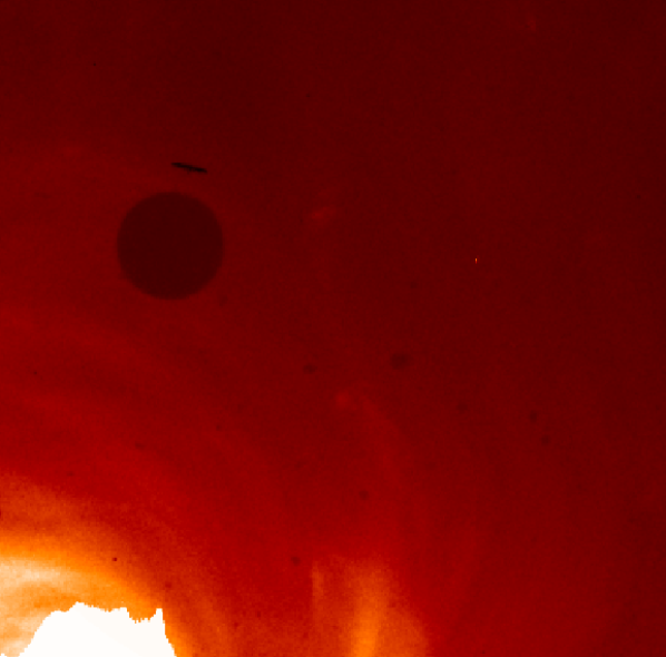
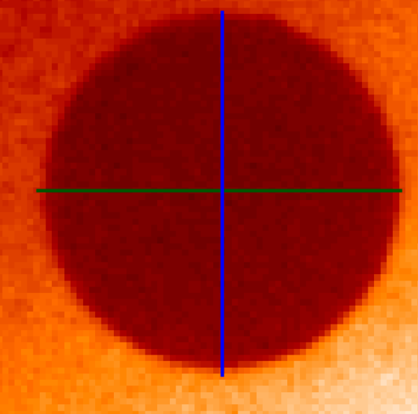
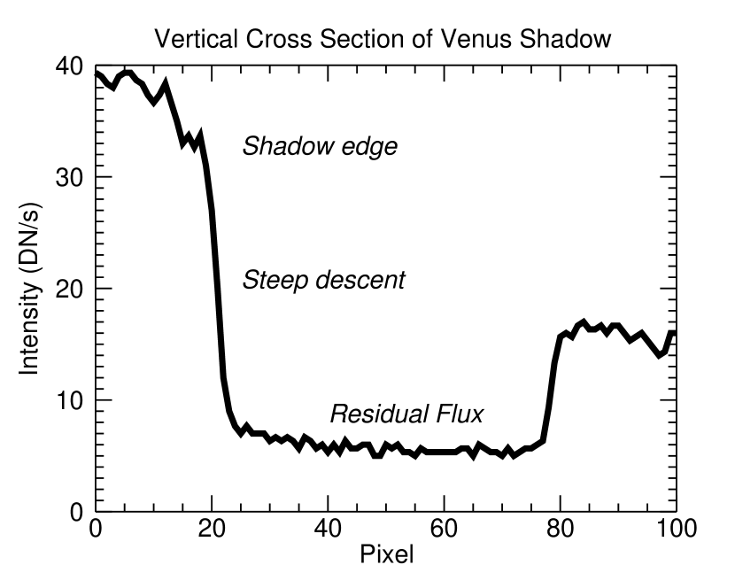
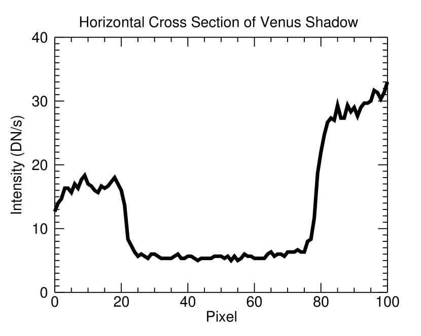
Figure 2: Top Left: Venus transit above the active region.
Top Right: Schematic view of horizontal (E-W) and vertical (N-S) strips, green and blue, respectively.
Bottom Left: Vertical IP of Venus’  shadow. Bottom Right: Horizontal IP of Venus’  shadow.

The regions of steep descent have smooth corners on either side because of the convolution of a step function with the PSF (Reale et al. 2015; Weber et al. 2007).
The X-Ray residual flux in Venus’  shadow appears too high to be compatible with background signal (Kobelski et al., 2014). We have superimposed in Fig. 3 the IPs taken at different times and positions of Venus on the solar disk. We did not align the borders of Venus, since the purpose here is only to show the level of residual flux (albeit not sampling regularly the whole transit).

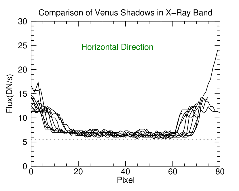
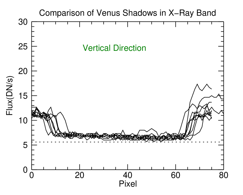
Figure 3: IP of Venus’  shadow in both horizontal (Left panel) and vertical (Right panel) directions at different times of observations and positions of Venus on solar disk.

As we can see the level of residual flux is high at any time; the intensity at the shadow’s edge strongly depends on the nearby (along the line of sight) solar emission near Venus at the time the specific frame was taken (Reale et al., 2015).
To check the effect of possible instrumental scattering in XRT across Venus’  shadow, especially when close to active regions, we took the average flux measured in three regions: in the Venus disk and in two concentric annuli around the Venus disk. Annulus 1 has inner radius $R_{v}$, namely the Venusian radius, and outer radius 2$R_{v}$, as shown in Fig. 4. Annulus 2 has inner and outer radii $R_{v}$ and 5$R_{v}$, respectively. We plotted the evolution of the mean flux inside each of these annular regions versus the time of observation ($T_{OBS}$) in Fig. 4, along with the flux measured in Venus’  shadow. In order to have a comparable time series in all light curves we chose $T_{OBS}=$ 2012-06-05T21:58:39.912 of one Hinode/XRT image as the reference time. Also, the time of Venus’  entrance onto the solar disk is marked with a red vertical line. For each data point the Poisson errors of DN (Digital Numbers) has been used as the error bars in the light curves. This amounts to assume a DN-to-photon conversion factor of 1; according to Narukage et al. (2011) such a factor applies to $T\sim 1.5$ MK, typical of the average, or quiet, corona. The conversion factor changes only slightly over the temperature range of interest for the non-flaring corona; since, also, the error depends on the square root of the photon number, the error bar determined is adequate even considering the multi-temperature corona

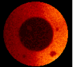
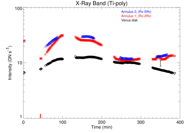
Figure 4: Left: Central Black circle: Venus disk; Red annulus: annulus 1 around the Venus disk.
Right: the evolution of mean X-ray flux inside Venus disk (Black), annulus 1 (Red) and annulus 2 (Blue) vs. T_OBS.
Annulus 1 has inner and outer radii R_v and 2R_v. Annulus 2 has inner and outer radii R_v and 5R_v. The vertical bar on the right shows the typical error size. The red vertical line in the lower left marks the first contact.

The initial high annulus flux is due to limb brightening, crossed during the initial phase of the Venus transit; then Venus gets close to a big active region, during the central phase of transit, and the mean flux of both the Venus disk and the annuli increases. (The maximum mean flux is measured in this phase.) As Venus moves away from the active region the flux decreases slowly. At the final stage, Venus completes the transit and touches the other limb with a small increase in mean flux at the end of all of the three curves. The blue curve does not cover the full data set: for some images, the annulus with the outer radius 5$R_{v}$ extends beyond the borders of the X-ray image.

3.2 Mercury IP Analysis

Since the atmosphere of Venus may contribute to — or be the cause of — the residual flux in IPs of Venus’  shadow, we considered the shadows of other celestial objects occulting the Sun but lacking an atmosphere, in order to remove the possible effects of atmosphere.
As a first choice we selected Mercury, already analyzed by Weber et al. (2007). If some effect due to PSF scattering is present in the case of Venus, it should be stronger in the case of the smaller Mercury disk: Mercury casts a shadow with an angular diameter of $\approx$ $10^{\prime\prime}$.
We have also made some analysis, not reported here, of the Moon’s shadow during solar eclipses observed with Hinode/XRT and found almost zero signal coming from the Moon’s X-ray shadow. In Fig. 5 we have plotted the IP of Mercury’s shadow in the X-Ray band, as taken through the Al-poly filter of XRT, along both the horizontal and the vertical directions. The relevant images were $384\times 384$ pixels large.

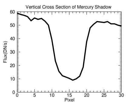
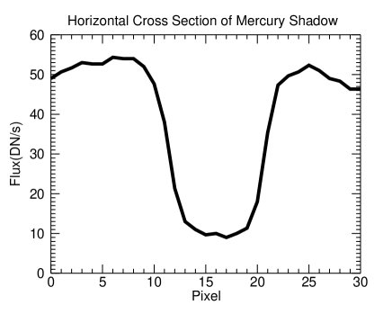
Figure 5: Left: Vertical IP of Mercury’s shadow. Right: Horizontal IP of Mercury’s shadow. Images taken through the Al-poly filter of XRT.

In the case of Mercury we initially find a residual flux, at a level comparable to that in Venus’  shadow, as well as a smooth profile. Therefore the effect appears to be, at first sight, the same for Venus and Mercury.
As a next step, in order to remove possible instrumental effects due to the PSF, we deconvolved Venus images using the Hinode/XRT PSF and other codes, and compared the relevant results. We also deconvolved Mercury images with the same tools to cross-check the results.

4 Deconvolution

Among different indirect methods of deconvolution such as least-squares fit, Maximum Entropy, Maximum likelihood (Starck et al., 2002), and Richardson-Lucy (Richardson 1972; Lucy 1974), we used the codes based on Maximum Likelihood (M-L) and Richardson-Lucy (AIA Richardson-Lucy; AIA) available in SolarSoft IDL libraries. For a short description of the codes that we used, please refer to Appendix B.
With the above codes and the Hinode/XRT PSF we performed deconvolution of the images, and then compared the results to pinpoint similarities and differences; the Venus Ti-poly images were $384\times 384$ pixels large. We repeated the cross section analysis, presented before, for the deconvolved images.

4.1 Deconvolution of Mercury shadows

Mercury and Venus have been observed at different times, in 2006 and in 2012 respectively, and with different filters. However our aim here is just to check the performance of the updated PSF in removing any emission concerning the instrumental scattering. The cross sections of Mercury shadow, before and after deconvolution, are presented in Fig. 6. After deconvolution, the cross section of Mercury’s shadow has practically zero residual flux with edges sharper than those of the original profiles.

Figure 6: Left: Mercury IP before (Black) and after deconvolution with the M-L code (Red).
Right: comparison between IP before (Black) and after deconvolution with AIA (Blue) and M-L (Red).

These results are very important since they not only confirm the accuracy of the updated Hinode/XRT PSF but show that, at least in the case of Mercury, the residual flux is due to PSF scattering. An analogous study was done by (Weber et al., 2007), with similar results, using a previous version of the PSF of Hinode/XRT.

4.2 Deconvolution of Venus shadows

Cross sections of Venus’  shadow after deconvolution are shown in Fig. 7.

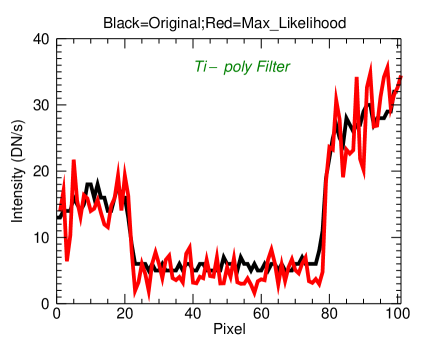
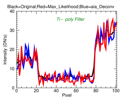
Figure 7: Left: Venus IP before (Black) and after deconvolution made with the M-L code (Red).
Right: Comparison between IP before (Black) and after deconvolution made with AIA (Blue) and M-L (Red).

.

These cross sections of Venus images deconvolved with the M-L and AIA codes show that:

$\bullet$

In some cases the cross sections of images deconvolved with the M-L code have more fluctuations in comparison to those obtained with the AIA code;

$\bullet$

For Venus, similarly to the Mercury case, the borders seem to be sharper after deconvolution;

$\bullet$

Residual flux is present in Venus images even after deconvolution; such a flux is significantly higher than the noise.

Residual flux present in Venus cross sections after deconvolution does not appear to be due to the Hinode/XRT PSF, since the accuracy of the PSF has been confirmed in the Mercury analysis. Being that the angular size of Mercury is considerably smaller than that of Venus, any effect of PSF scattering should manifest itself more in the Mercury cross sections.
Since both the M-L and AIA codes are iterative we changed the number of iterations during the deconvolution process for some images in each dataset to check the effect of iteration, especially to see whether increasing the number of iterations led to the residual flux being further decreased or removed. The trend is that with increasing the number of iterations the residual flux is still present and its mean value for any reasonable number of iterations is very constant, except that with increasing iterations the fluctuations increase in the IPs. Generally the M-L code is more sensitive to noise and the quality of the images.
So the presence of a significant residual flux in Venus’  shadow is not due to instrumental scattering but should be related to Venus; for instance, it could originate from some effect occurring in Venus’  atmosphere.
Comprehensive analysis of deconvolutions show that:

$\bullet$

The AIA code does not conserve the total flux, yielding curves with 15% of total flux, so for each image we readjusted the amplitude to conserve the total flux;

$\bullet$

Deconvolution causes artifacts and spurious “spikes” at the edge (borders), a common problem in deconvolution which, in the case of Venus, are well identified and do not affect the evaluation of the average flux in the shadow (cf. Fig. 7).

We again followed the evolution of the flux in Venus’  shadow and in two reference annuli, as done in Section 2, after deconvolution. We plotted the evolution of mean flux inside each of these three regions versus T_OBS in Fig. 8. The space-averaged fluxes obtained after deconvolution with the two methods are virtually the same resulting in three light curves, each being two superimposed.

Figure 8: Evolution of mean Ti-poly flux after deconvolution: inside Venus disk with AIA (Black) and M-L (Red) codes; inside annulus 1 with AIA (Green) and M-L (Red) codes; inside annulus 2 with AIA (Blue) and M-L (Red) codes. The bar on right shows typical error sizes. The red vertical line in the lower left marks the first contact.

The most important points in Fig. 8 are:

$\bullet$

The amount of mean flux inside Venus’ disk after deconvolution has decreased slightly, especially where close to the active region, therefore deconvolution appears to have removed just a small amount of X-ray flux from Venus’  shadow;

$\bullet$

The mean fluxes inside the two annuli have not changed after deconvolution (cf. also Fig. 7);

$\bullet$

We see that the flux inside Venus’  shadow and that inside the two annuli gradually rise as Venus gets more and more inside the solar disk and decreases thereafter; however the flux inside Venus’  shadow is not strictly correlated to that inside the two annuli.

$\bullet$

There may be some relationship between the observed residual flux and the high surrounding flux;

$\bullet$

The mean flux value for both the AIA and M-L deconvolution codes are virtually the same despite the fact that the profiles for the deconvolved images are not the same.

As an additional test on the error, we have determined the standard deviation of the residual flux values inside Venus disk and found that it varies between 0.4–1.0 DN s^-1, which is negligible in comparison to the observed residual flux ($>$ 5 DN s^-1).

5 Light Leak Contamination

5.1 Light Leak Effect on XRT Filters

An increase in XRT’s straylight was detected on May 9th of 2012, shortly before the Venus transit (5th–6th June 2012), which causes significant visible light contributions to the X-Ray images in some filters. In addition, a sudden increase of intensity by a factor of 2 was observed in the visible light measurements (i.e., in the G-band channel). At the same time, the XRT team recognized wood-grain like stripes in daily images taken with the Ti-poly filter (Takeda et al., 2016). The team believes the increase of visible straylight to have been caused by a pinhole puncture in the entrance aperture filters.
The analysis showed that the light leak affects only some of the X-Ray filters: a minor effect was detected for the Al-mesh and Al-poly filters but it was very small ($\leq\leavevmode\nobreak\ 5$ DN s^-1), while it strongly affected the Ti-poly and C-poly filters (Takeda et al., 2016).
In order to exclude the possibility that Venus residual flux in Ti-poly could be due to the straylight, we used data collected with the Al-mesh filter to repeat the analysis. Importantly, the light leak has a very small effect on the Al-mesh filter, to such a level that it can be neglected (Takeda et al. 2016).

5.2 Al-mesh Filter Analysis

In Fig. 9 we present a typical IP of Venus’  shadow in both horizontal and vertical directions, taken in an image collected with the Al-mesh filter.

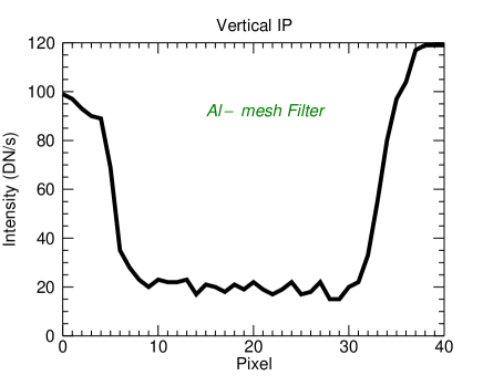
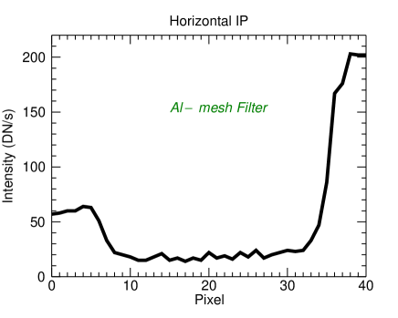
Figure 9: Left: Vertical IP of Venus’  shadow. Right: Horizontal IP of Venus’  shadow. (XRT Al-mesh filter)

.

As we can see:

$\bullet$

The residual flux is still present in all IP plots.

$\bullet$

The intensity profiles of the Al-mesh filter appear approximately 3-5 times higher than Ti-poly ones; the reason is that Al-mesh images are binned $2\times 2$ while Ti-poly data are binned $1\times 1$ and the filters have different transmissivity; the Al-mesh images are $192\times 192$ pixels large.

Also for Al-mesh data we deconvolved images to remove any effect due to the PSF scattering. Sample IP results, after deconvolution, are shown for the vertical direction in Fig. 10.

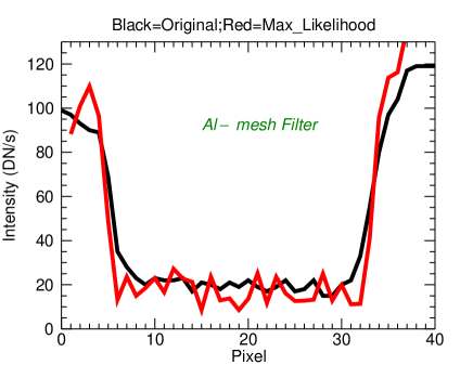
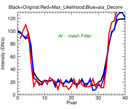
Figure 10: Left: Venus IP before (Black) and after deconvolution with M-L code in the vertical direction (Al-mesh filter).
Right: comparison of IP before (Black) and after deconvolution with AIA (Blue) and M-L (Red) in vertical direction.

Deconvolution analysis shows that:

$\bullet$

Artifacts and spurious “spikes” at the edges (borders) of the IPs are much stronger in Al-mesh images in comparison to Ti-poly images.

$\bullet$

The AIA code does not conserve the total flux, yielding curves with 60% of total flux (in Ti-poly, 15%), so for each image we rescaled the amplitude to conserve the total flux.

$\bullet$

The most important fact is that even after deconvolution residual flux is still present in all of the IPs and is significantly higher than the noise.

We have also determined the evolution of the flux in Venus’  shadow after deconvolution for Al-mesh images and in two reference annuli, similarly to what we have done for the Ti-poly data. Fig. 11 shows the evolution of the mean flux inside each of these regions versus T_OBS.
Also for Al-mesh data the DN to photon conversion factor of 1, used to derive the error bars, is appropriate to $T\sim 1$ MK and changes slowly over the T range of interest for the non-flaring corona.

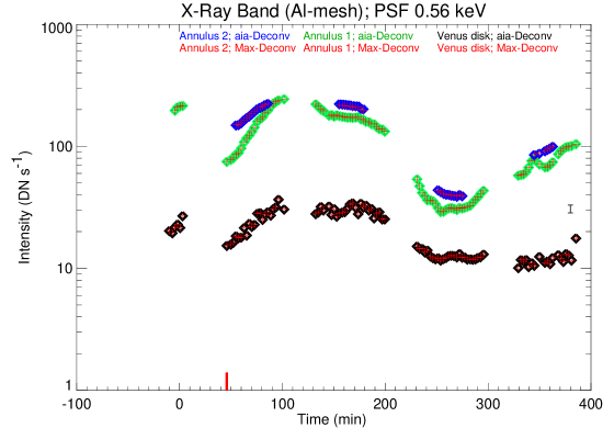
Figure 11: Evolution of mean X-ray flux (as measured through Al-mesh filter) inside Venus disk after deconvolution with AIA (Black) and M-L (Red) codes, inside annulus 1 after deconvolution with AIA (Green) and M-L (Red) codes, and inside annulus 2 after deconvolution with AIA (Blue) and M-L (Red) codes. A typical error bar is shown on the right. The red vertical line in the lower left marks the first contact.

The ratio of the maximum value of flux inside annulus 1 to the lowest one for Al-mesh data is slightly more than 5, on the average. The ratio is different from that of Ti-poly ($\approx 3$) probably because the light leak effects (if any) are very small in the case of Al-mesh.
We can safely state that the flux detected in Venus’ dark side most likely is not due to PSF scattering, noise or light leak, but it may originate from some phenomenon related to Venus.

6 The EUV and UV Flux Analysis

We have done a similar analysis of IPs of Venus’  shadow in the UV and EUV bands. An image of Venus transit and a sample cross section in the EUV band, taken with SDO/AIA at 193 Å, is shown in Fig. 12.

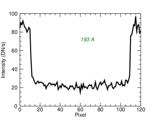
Figure 12: Image in the EUV band (193 Å) of Venus transit (Left) and its horizontal IP (Right).

Similarly to what was done for the X-Ray band, we deconvolved the EUV images to remove the effects of the PSF. Various works have been dedicated to deriving the PSF of SDO/AIA. Grigis et al. (2012) derived the PSF using pre-flight and post-flight measurements and calibrations. Poduval et al. (2013) derived the in-flight SDO/AIA PSF using several observations, including some of the Moon’s limb made during a solar eclipse observed with SDO/AIA. González et al. (2016) used observations of both a solar eclipse and a Venus transit to derive the SDO/AIA PSF. These authors assumed that there is no emission coming from the dark side of Venus during the transit, but then discovered that they needed to include a long range effect, otherwise the parametric PSF they used would not be able to remove “the apparent emission inside the disk of Venus”.
Interestingly, in a similar but unrelated study, DeForest et al. (2009) used the 2004 Venus transit to determine the TRACE in-flight PSF. They, too, assumed that no EUV radiation comes from Venus’ dark side, and then found that “much more scattered light is found than can be accounted for merely by diffraction” and that half of the scattered light was due to some other mechanism.
It is quite possible that both González et al. (2016) and DeForest et al. (2009) had discovered, and were trying to account for, some real EUV emission of the kind we find.
For the above reasons we decided to adopt the PSF derived in Grigis et al. (2012), which is available in SSW and is a standard in deconvolving AIA EUV images. We have also applied the Poduval et al. (2013) PSF, kindly provided by the author, to test if results are different. This latter PSF is not available for full disk images so we have compared the results obtained with SSW and Poduval PSF only for partial disk images; we found that we get in practice the same average flux with the standard deconvolution in SSW and with the deconvolution which uses Poduval PSF. Being reassured by this result, we resorted to the Grigis et al. (2012) PSF to deconvolve full disk images. We concentrated on full disk images (albeit their number is smaller) because we are thereby certain to remove even possible long range effects.
We have, thus, deconvolved each full disk image with the PSF available in SSW and derived the average flux in Venus shadow and in annulus 1. In Fig. 13 we show the evolution of the UV and EUV average flux values as observed with SDO/AIA in the dark side of Venus and in the smallest annulus (annulus 1) taken around Venus, before and after deconvolution performed with the AIA routine and with the Maximum Likelihood (M-L) routine.
The data in the 335 Å band show an unusual behaviour with deconvolution: the average flux inside Venus’ disk increases after deconvolution, just the opposite of what one expects and which happens in any other band. The flux in Venus’ shadow is rather low before deconvolution, so any signal that is present and not due to noise must be marginal. Indeed, the signal after deconvolution is virtually constant. We are thus forced to consider the results for 335 Å images as unreliable; we present all the relevant results just for completeness and as an additional null test, but these results are of little relevance for our problem.
No PSF is available for the 1700 Å band, so we cannot deconvolve the relevant data; we simply used the non-deconvolved data.

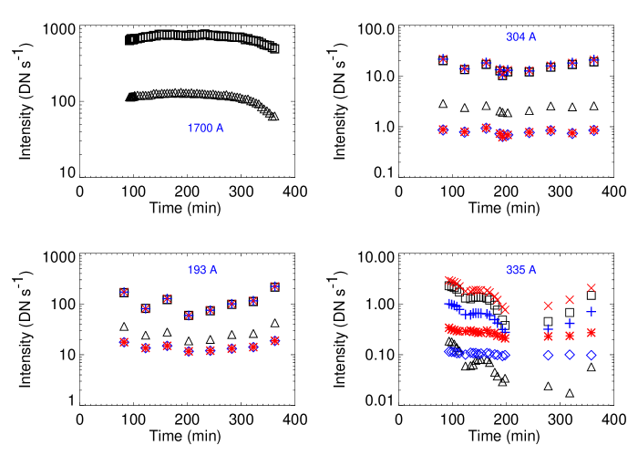
Figure 13: Mean flux evolution inside Venus disk and annulus 1, before and after deconvolution vs. time in UV and EUV bands. Top Left: 1700 Å; Top Right: 304 Å; Bottom Left:193 Å; Bottom Right: 335 Å. Black square: annulus average flux before deconvolution, red X : annulus average flux after ML deconvolution, blue cross: same as red X but after aia deconvolution, black triangle: Venus disk average flux before deconvolution, red star: Venus disk average flux after M-L deconvolution, blue diamond: Venus disk average flux after aia deconvolution.

It is immediately apparent that the flux evolution in any EUV band has no evident correlation with that of the X-Ray flux; in the 1700 Å band the flux increases as Venus crosses the solar disk, and decreases thereafter. In the 335 Å and 193 Å bands the opposite occurs; few changes are seen in the 304 Å band. However it appears that also in these cases the flux in the shadow clearly follows that in the surrounding ring, almost (but not exactly) by a fixed factor.
This approximate proportionality of the flux in Venus’  dark side relative to the surrounding regions hints at a strong analogy between the mechanisms generating Venus’  dark side emission in X-ray, EUV and UV bands.
Fig. 14 shows the evolution of the ratio between flux values inside the annulus and in the Venusian disk, for the original data and for the images deconvolved with both methods.

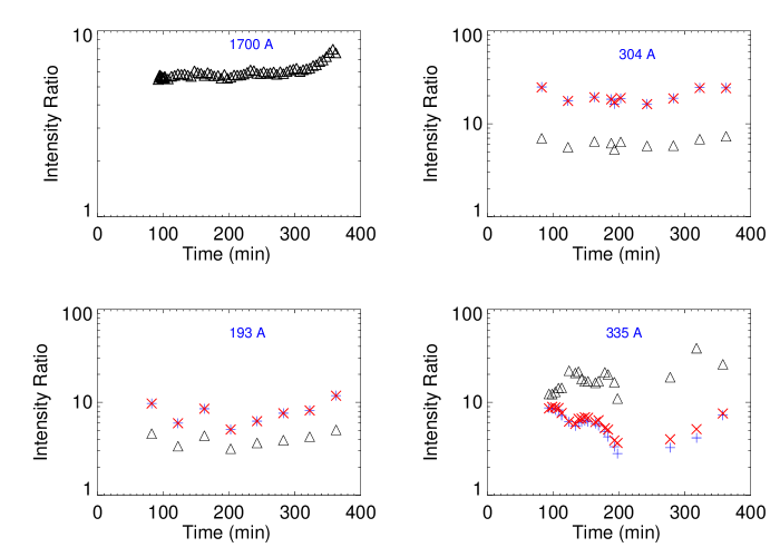
Figure 14: Evolution of (mean annulus 1 flux to mean Venus disk flux) ratio before and after deconvolution in UV and EUV bands. Top Left: 1700 Å; Top Right: 304 Å; Bottom Left:193 Å; Bottom Right: 335 Å. Black Triangle: Ratio before deconvolution; Blue cross: Ratio after aia deconvolution; Red X: Ratio after ML deconvolution.

Fig. 15 shows the minimum, maximum and mean values of the ratio between flux values inside the annulus and in the Venus disk versus wavelength and versus temperature (of the plasma which would be observed on the Sun). Since any possible deconvolution would slightly decrease the flux in Venus disk also at 1700 A, we may expect that the data points at 1700 are higher. There appears to be a slight increasing trend with wavelength.

Figure 15: Minimum, maximum and mean values of the ratio between the average intensity on solar disk around Venus and average flux inside Venus’  shadow vs. wavelength (left panel) and vs. solar plasma temperature (right panel).

7 Conclusion

We studied the Venus transit across the solar disk which occurred in 2012 and was observed with Hinode/XRT in the X-Ray band and SDO/AIA in the EUV and UV bands. We have measured a significant X-Ray residual flux from Venus’  dark side (i.e., from the Earth-facing side) during the transit that was significantly above the estimated noise level of 2 DN s^-1, as reported by Kobelski et al. (2014).
Let us discuss the systematic uncertainties of XRT flux. According to Kobelski et al. (2014) there are two kinds of systematic uncertainties for XRT. The first are those which have a reliable quantitative correction procedure such as: dark current, Fourier, vignetting, and JPEG compression noise sources; their correction procedures have been successfully embedded in xrt_prep.pro (the calibration reformatter). Since all of the data we have used for X-ray analysis (both Ti-poly and Al-mesh filters) have been prepared with xrt_prep.pro, we expect that this class of uncertainties has been properly corrected and does not explain the observed residual.
The second kind of systematic uncertainties are model-dependent and are not included in xrt_prep.pro; among them are light scattering by the grazing-incidence mirror of XRT, visible straylight leak and photon counting uncertainty (Kobelski et al., 2014). In this respect the error bars for each flux value have been computed as follows. From the flux values, the exposure times, and the conversion factor from DN to photons, we have computed the number of photons collected and from them the statistical errors due to Poisson noise. This statistical error has been converted to a flux error bar per data point. The resulting error bar is typically less than the 2 DN s^-1 mentioned by (Kobelski et al., 2014). In sections 4 and 5 we comprehensively discuss the PSF scattering and visible light leak effects.
To test the performance of the instrument’s PSF (i.e., due to instrumental X-ray scattering) and the possible effect of the atmosphere on the residual flux, we studied a Mercury transit across the solar disk, observed with the Hinode/XRT in 2006. We measured an apparent X-Ray residual flux in the case of Mercury before deconvolution.
For both Venus and Mercury we used a new version of the Hinode/XRT PSF, selected well illuminated images in the X-Ray band, and deconvolved them. Even after deconvolution, flux from Venus’  shadow has remained significant, while in the Mercury case it has become negligible. So it appears that the observed flux in Venus’  shadow is real.
As for the Venus case, we have analyzed two X-ray datasets: a set collected with Ti-poly filter and another collected with Al-mesh filter. While the former is potentially strongly affected by a light leak that appeared a short time before that Venus transit, the latter is not. Both datasets, however, clearly show the presence of a significant flux from Venus’  dark side, showing the reality of this effect. Although we consider the results from the Al-mesh data set to be a strong confirmation for the observed X-Ray residual flux, the Ti-poly results also provide more confidence about the observed residual flux and prove this effect in more than one filter. The level of the residual flux is not constant: as Venus crosses the solar disk it gradually grows, reaching a maximum roughly halfway through the transit, and then gradually decreases as it approaches the solar limb. The flux changes by an almost fixed factor of the flux of the surrounding solar regions (i.e., along nearby lines of sight) as shown in Figs. 8 and 11. On the other hand the use of the PSF and the test on Mercury convincingly shows the removal of any PSF effect. Furthermore, any light leak effect would instead be expected to be almost uniform or constant in time.
The PSF of XRT has also been determined at 1.0 keV. We find that deconvolving the images with this PSF reduces by a factor of about 0.5, on average, the flux inside the Venusian disk. More specifically, the mean flux across the disk before deconvolution is about 24 DN s^-1. After deconvolution with the 0.56 keV PSF model it is about 20 DN s^-1, but after deconvolution with the 1.0 keV PSF model it is about 10 DN s^-1. Therefore a significant flux level still remains, even after deconvolution with the 1.0 keV PSF, showing the reality of the effect nonetheless.
In this respect, however, we believe that the PSF at 0.5 keV is more appropriate to our study. In fact, we are detecting photons coming from the corona and re-processed at Venus or in Venus’  magnetotail (or something related to Venus), a process which should not raise photon energy. The corona is at a few MK (at most 3 or 5, and only then in some places like active region cores), and no flare appears during the Venus transit. So a relatively smaller fraction of photons are expected even at 0.56 keV. We use the Al-mesh and Ti-poly filters; so considering the coronal spectrum folded with the Al-mesh filter response (Al-mesh data are the most reliable ones for Venus X-ray observations), we may shift the average of the observed plasma emission some 0.1 keVs closer to, but not at, 0.56 keV. On one hand we are confident that the general result is robust against the choice of PSF model, but the use of the 0.56 keV PSF can be considered to be a conservative evaluation, and so we can use the relevant results quite safely.
The analogous kind of analysis made in four EUV bands observed with SDO/AIA has shown that there is also some flux in these bands coming from Venus’ night side, and that its evolution clearly follows that of the flux inside an annulus surrounding Venus. The light curves do not show, however, any trend similar to that of the X-Ray flux.
Past X-ray observations of Venus were very different, in many respects. In January 2001, Venus was observed for the first time with the Chandra X-ray telescope. Dennerl (2002) proposed that the fluorescent scattering of solar X-rays from Venus’  atmosphere was the primary source of the X-ray emission they observed. Not only the morphology, but also the observed X-ray luminosity was consistent with the scattering of solar X-rays (Dennerl, 2002).
In 2006 and 2007 again with Chandra, besides fluorescent scattering, Solar Wind Charge eXchange (SWCX) emission was clearly detected. Comparison of X-ray images taken in 2006 and 2007 with those obtained in 2001 (taken at a similar phase angle) showed that the limb brightening had increased. This would be the case if the X-ray radiation from Venus was the superposition of scattered solar X-rays and SWCX emission. The lack of detection of any SWCX-induced X-ray halo in the first Venus observation was explained by being during a high level of the solar X-ray cycle (Dennerl, 2008).
Previous X-ray observations, however, have shown X-ray emission from the sunlit side of Venus. The low intensity we detect in X-ray and EUV comes from the dark side of Venus, and appears to have a totally different origin; it appears to evolve during the transit remaining, at any time, approximately proportional to the emission of the solar regions along nearby lines of sight. This intensity cannot be due to scattering in the upper atmosphere of Venus because we should detect a brighter inner rim in Venus’  shadow.
The effect we are observing could be due to scattering or re-emission occurring in the shadow or wake of Venus. One possibility is due to the very long magnetotail of Venus, ablated by the solar wind and known to reach Earth’s orbit (Grünwaldt et al., 1997). This magnetotail could be side-illuminated from the surrounding regions and could scatter, or re-emit, the radiation; the cone of Venus shadow reaches up to $9.6\times 10^{5}$ km away from Venus, leaving ample space ($\approx 4.5\times 10^{7}$ km) for side-illuminating the magnetotail. The emission we observe would be the reemitted radiation integrated along the magnetotail.
One wonders if such an effect is important for exoplanets, in particular for those Jupiter-size planets orbiting very close to their stars; they may have a very large ablated tail, especially if they do not have a magnetic field. To some extent, the study of these tails may help to understand, among other issues, the presence (or lack thereof) of magnetic fields.
Future work will study in more detail this phenomenon: we plan to study some faint structures present in the shadow and address possible physical mechanisms involved in generating the residual emission.

APPENDIX A

Metrology data and on-orbit observations are used to model the point spread function of the X-Ray Telescope’s (XRT; (Golub et al., 2007)) mirror assuming that XRT is operated at the best on-axis focus. The metrology data estimate encircled energy profiles for two energies, 0.56 keV and 1.0 keV. We develop a PSF for both energies and find the function that returns the encircled energy data as a piecewise continuous function composed of a Lorentzian core and a series of power-law functions as its wings. The PSFs we develop do not consider other sources of scattering such as the effects of changing the focus position, other elements within the optical system, filters, and the CCD camera system, or material contamination on the XRT CCD. We do not incorporate any non-axisymmetric structures although the system PSF is known to vary (see Fig. 4 in Golub et al. (2007)).
The XRT mirror is a Wolter Type-I grazing incident optic built by Goodrich. The XRT has 9 broadband filters that sample plasma temperatures from 0.5–10 million Kelvin and is equipped with a 2048x2048 CCD. The XRT has 1.02860 arcsec pixels with a wide field of view of 34x34 arcmin (Kano et al., 2008). The mirror manufacturer provided encircled energy estimates based on the Power Spectral Density (PSD) derived from measurements of the mirror surface roughness.
We construct two PSFs for the XRT mirror using a semi-empirical approach. We model the core of the PSF by considering a variety of functions that could reproduce the on-axis encircled energy data. We then estimate the wings of the PSF based on scattering patterns observed in XRT data. The wings of the PSF are modeled assuming a piecewise continuous power law of the form:

$$P_{i}(r)=r^{-\alpha_{i}},{\rm where\ }{\alpha_{i}}\geq 0,{\rm and\ }{\alpha_{i+1}}\geq{\alpha_{i}},$$

where $r$ is the radial distance from the optical axis. We assume the PSF is spatially invariant and only depends on the radial distance from the scattering source. Scattered light from XRT data are used to determine the breakpoints of the function so that the following criteria are met:

1. The metrology data affirms that 81% of the encircled energy lies within 5 arcsec for a 0.56 keV source and 77% for a 1.00 keV source, meeting design specifications.

2. The wings of the PSF match and extend the slope of the encircled energy in a smooth and continuous way.

3. In the case when the PSF will be normalized, we assume that 100% of the light will be scattered within the XRT field of view.

To gauge how light is scattered far from the source we use full frame images of (a) limb flare data in which a bright flare occurs on the solar limb when the Sun is centered in the field of view, and (b) solar eclipse data when the Moon passes between XRT and the Sun. Because of Hinode’s orbit, XRT experiences either a partial or total solar eclipse twice a year and XRT takes full disk data in several filters. We use the Moon as a way to measure scattered light when it partially obscures an active region on the Sun. Scattered light from these bright regions is easily visible across the Moon’s shadow.
In addition to the scattered light from the mirror, there are at least two other causes of scattered light. First is the scattering due to the entrance apertures that is accentuated during a solar flare, and the second is a pattern of scattered light that is pointing dependent and is always present. The left panel of Fig.16 shows an example of solar eclipse data used in the analysis and demonstrates both patterns of scattered light within the Moon’s shadow.

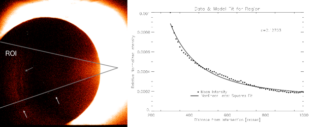
Figure 16: Left: Hinode XRT C-Poly (log intensity) eclipse image taken 2008 February 7 at 5:17:53 UT. White arrows point to the shadow of the entrance filters and the gray arrow points to the azimuthal scattered light pattern. Right: Plot of the mean relative normalized intensity as a function of distance from the intersection of the two lines within the region of interest (ROI). Within the ROI, the scattered light follows an inverse square law up through the gray arrow when the intensity increases again. This fit does not distinguish between the mirror scatter and the azimuthal scatter.

The image is scaled on a log scale with pixel values above a few DN s^-1 saturated to white so that the low-level scatter can easily be seen. Dark bands that appear to emanate from the scattering source are the pattern created from the entrance filters (white arrows). A gray arrow points to the second scattering pattern. It is a partial dark ring followed by a region of bright light. They appear as partial bands around the scattering source. This pattern is pointing dependent and changes location depending on pointing and the location of the scattering source within the field of view.
All XRT data are processed using the standard reduction routines provided by the XRT team in SolarSoft. We use full resolution images. The exposure times of the data vary between 0.5–16 seconds depending on the solar conditions. To estimate the amount of scatter in an XRT image, the average normalized intensity along an arc as a function of radial distance from the scattering source is fit to the general power law function of the form:

$$P(r)=\alpha(r-b)^{-c}+d,$$

where $a$, $b$, $c$, and $d$ are all free parameters. The intensity is normalized to the maximum value set by the data reduction routine, xrt_-prep.pro. This fitting method is not able to distinguish between the different sources of scatter.
To mitigate the effects of the scattering due to the entrance filters, we select a region between dark bands of scattered light. An example of a region is the one between the two lines on the image on the left of Fig.16. We attempt to deal with the second source of scattered light by considering regions closer to the scattering source rather than farther away.
The encircled energy data imply the wings of the PSF do not significantly contribute to the encircled energy far from the center. At a radial distance of 4–5 arcsec there is little increase in the encircled energies. Therefore, we expect that far from the source, the other scattering elements will dominate the scattering.
We use Mathematica to calculate the encircled energy curves for both PSF models, corresponding to the two energy channels, over a spatial grid that is appropriate for the meteorology data and that oversamples the instrument plate scale. Fig.17 shows the encircled energy measurements (squares) for 0.56 keV (a) and 1.0 keV (b).

Figure 17: Encircled energy plot of the manufacturer data (squares), the model PSF (dashed line) and the model discretized for XRT pixel size (solid line) for 0.56 keV, (a) and 1.0 keV (b).

For each of the datasets, we find that a single function could not reproduce the given encircled energies. The two energies have the same functional form but have different parameter values and breakpoints; the relevant values are given in Table 2. We find the inner portion of the PSF is best represented by a Lorentzian function out to an inner radius, $r_{0}$. From $r_{0}$ to 5 arcsec, the $r^{-1}$ function returns the correct encircled energy measurements.
We then use the assumption that the PSF will continue to follow the power law trend and fit the following model:

$$P(r)=\begin{cases}a\frac{exp(-\frac{r^{2}}{\sigma^{2}})}{\gamma^{2}\>+\>r^{2}},&r\leq r_{0};\\ br^{-1},&r_{0}\leq r\leq r_{1};\\ cr^{-2},&r_{1}\leq r\leq r_{2};\\ dr^{-4},&r_{2}\leq r\leq\infty.\end{cases}$$

Table 2: Normalized PSF parameter values.
* Denotes exact values and not approximations.

Parameter Values	0.56 keV	1.0 keV
$\sigma$	2.19256	2.36982
$\gamma$	1.24891	0.914686
a	1.31946	0.847955
b	0.03*	0.038*
c	0.15*	0.19*
d	18.4815* r0	20.1571* r0
r0	3.4167	3.22857
r1	5*	5*
r2	11.1*	10.3*

A plot of the encircled energy (squares) for both channels is given in Figure 2 along with the model PSF (black lines). The models fit the data well. We also discretized the models to the XRT pixel size (solid line).
A simple calculation is applied to consider the relative applicability of the two PSF models for a range of typical plasma temperatures in the corona. We make use of the Astrophysical Plasma Emission Code (APEC, Smith et al. (2001)) to model the plasma emission as a function of wavelength and temperature. We fold this model through the XRT’s spectral response and convert the instrument spectral response to a temperature response for each of XRT’s filters. We create a spectral response of several plasma temperatures and compare the amount of energy at or below 0.75 keV to the amount of energy above 0.75 keV for a given temperature plasma. Table 3 shows the relative spectral response for each of the XRT’s filters.

Table 3: Relative spectral response for each of the XRT’s filters assuming the specified temperature.

	1MK	1MK	3MK	3MK	5MK	5MK	10MK	10MK
Filter	$\leq$ 750ev	$>$ 750ev	$\leq$ 750ev	$>$ 750ev	$\leq$ 750ev	$>$ 750ev	$\leq$ 750ev	$>$ 750ev
Al-mesh	0.98	0.02	0.23	0.77	0.07	0.93	0.04	0.96
Al-poly	0.95	0.05	0.17	0.83	0.05	0.95	0.03	0.97
C-poly	0.95	0.05	0.13	0.87	0.03	0.97	0.01	0.99
Ti-poly	0.96	0.04	0.13	0.87	0.03	0.97	0.02	0.98
Be-thin	0.62	0.38	0.02	0.98	0.00	1.00	0.00	1.00
Be-med	0.08	0.92	0.00	1.00	0.00	1.00	0.00	1.00
Al-med	0.04	0.96	0.00	1.00	0.00	1.00	0.00	1.00
Al-thick	0.00	1.00	0.00	1.00	0.00	1.00	0.00	1.00
Be-thick	0.00	1.00	0.00	1.00	0.00	1.00	0.00	1.00

Table 3 shows that, for plasma temperatures above 1MK, a significant portion of the signal will come from energies greater than 0.75 keV.
The PSFs provided above are designed with normalization in mind but this condition is not necessary, and in fact it forces that 100% of the energy is scattered within the XRT field of view. With this condition relaxed, the PSF will scatter light far from the field of view. Table 4 provides the PSF models without normalization. The only difference between these and the normalized models is the value of $r_{2}$. This causes the slope of the encircled energy to essentially remain flat beyond 5 arcsec.

Table 4: PSF model without Normalisation.
* Denotes exact values and not approximations.

Parameter Values	0.56 keV	1.0 keV
$\sigma$	2.19256	2.36982
$\gamma$	1.24891	0.914686
r0	3.4167	3.22857
a	1.31946	0.847955
r1	5*	5*
b	0.03*	0.038*
c	0.15*	0.19*
D	7.35* r0	10.1251* r0
r2	7	7.3
EE at edge of FOV	93%	93%

APPENDIX B

Among different indirect methods of deconvolution available in SolarSoft IDL libraries, we used codes based on the Maximum Likelihood and Richardson-Lucy methods:

$\bullet$

AIA_ DECONVOLVE_ RICHARDSONLUCY.pro (AIA) based on Richardson-Lucy algorithm.
/darts.isas.jaxa.jp/pub/ssw/sdo/aia/idl/psf/PRO/aia_deconvolve_richardsonlucy.pro

The Richardson-Lucy algorithm in this code follows closely the algorithm discussed by Jansson (1997).

$\bullet$

MAX_LIKELIHOOD.pro (M-L) based on Maximum likelihood algorithm.
idlastro.gsfc.nasa.gov/ftp/pro/image/max_likelihood.pro
Based on papers by Richardson (1972) and Lucy (1974).

References

- Bentley & Freeland (1998) Bentley, R. D. & Freeland, S. L. 1998, in ESA Special Publication, Vol. 417, Crossroads for European Solar and Heliospheric Physics. Recent Achievements and Future Mission Possibilities, 225
- DeForest et al. (2009) DeForest, C. E., Martens, P. C. H., & Wills-Davey, M. J. 2009, ApJ, 690, 1264
- Dennerl (2002) Dennerl, K. 2002, A&A, 394, 1119
- Dennerl (2008) Dennerl, K. 2008, Planet. Space Sci., 56, 1414
- Freeland & Bentley (2000) Freeland, S. & Bentley, R. 2000, SolarSoft, ed. P. Murdin
- Grigis et al. (2012) Grigis, P., Yingna, S., & Weber M. for the AIA team. 2012, AIA PSF Characterization and Image Deconvolution Version 2012-Feb-13 - part of the SSW manual, in http://hesperia.gsfc.nasa.gov/ssw/sdo/aia/idl/psf/DOC/psfreport.pdf
- Golub et al. (2007) Golub, L., Deluca, E., Austin, G., et al. 2007, Sol. Phys., 243, 63
- González et al. (2016) González, A., Delouille, V., & Jacques, L. 2016, Journal of Space Weather and Space Climate, 6, A1
- Grünwaldt et al. (1997) Grünwaldt, H., Neugebauer, M., Hilchenbach, M., et al. 1997, Geophys. Res. Lett., 24, 1163
- Jansson (1997) Jansson, P. A. 1997, Deconvolution of images and spectra.
- Kano et al. (2008) Kano, R., Sakao, T., Hara, H., et al. 2008, Sol. Phys., 249, 263
- Kobelski et al. (2014) Kobelski, A. R., Saar, S. H., Weber, M. A., McKenzie, D. E., & Reeves, K. K. 2014, Sol. Phys., 289, 2781
- Lemen et al. (2012) Lemen, J. R., Title, A. M., Akin, D. J., et al. 2012, Sol. Phys., 275, 17
- Lucy (1974) Lucy, L. B. 1974, AJ, 79, 745
- Narukage et al. (2011) Narukage, N., Sakao, T., Kano, R., et al. 2011, Sol. Phys., 269, 169
- Pesnell et al. (2012) Pesnell, W. D., Thompson, B. J., & Chamberlin, P. C. 2012, Sol. Phys., 275, 3
- Poduval et al. (2013) Poduval, B., DeForest, C. E., Schmelz, J. T., & Pathak, S. 2013, ApJ, 765, 144
- Reale et al. (2015) Reale, F., Gambino, A. F., Micela, G., et al. 2015, Nature Communications, 6, 7563
- Richardson (1972) Richardson, W. H. 1972, Journal of the Optical Society of America (1917-1983), 62, 55
- Smith et al. (2001) Smith, R. K., Brickhouse, N. S., Liedahl, D. A., & Raymond, J. C. 2001, ApJ, 556, L91
- Starck et al. (2002) Starck, J. L., Pantin, E., & Murtagh, F. 2002, PASP, 114, 1051
- Takeda et al. (2016) Takeda, A., Yoshimura, K., & Saar, S. H. 2016, Sol. Phys., 291, 317
- Weber et al. (2007) Weber, M., Deluca, E. E., Golub, L., et al. 2007, PASJ, 59, S853