Random Neighborhood Graphs as Models of Fracture Networks on Rocks: Structural and Dynamical Analysis

Abstract

We propose a new model to account for the main structural characteristics of rock fracture networks (RFNs). The model is based on a generalization of the random neighborhood graphs to consider fractures embedded into rectangular spaces. We study a series of 29 real-world RFNs and find the best fit with the random rectangular neighborhood graphs (RRNGs) proposed here. We show that this model captures most of the structural characteristics of the RFNs and allows a distinction between small and more spherical rocks and large and more elongated ones. We use a diffusion equation on the graphs in order to model diffusive processes taking place through the channels of the RFNs. We find a small set of structural parameters that highly correlates with the average diffusion time in the RFNs. We found analytically some bounds for the diameter and the algebraic connectivity of these graphs that allow to bound the diffusion time in these networks. We also show that the RRNGs can be used as a suitable model to replace the RFNs in the study of diffusion-like processes. Indeed, the diffusion time in RFNs can be predicted by using structural and dynamical parameters of the RRNGs. Finally, we also explore some potential extensions of our model to include variable fracture apertures, the possibility of long-range hops of the diffusive particles as a way to account for heterogeneities in the medium and possible superdiffusive processes, and the extension of the model to 3-dimensional space.

1 Introduction

It could be argued that in any system transporting mass and energy there should be an underlying network responsible for conducting the materials through space. The flow of fluids of petrochemical interest obeys this general rule, where the role of the transporting network is played by the system of rock fractures. The study of rock fracture systems have a long tradition in hydrocarbon geology and hydrogeology due to the role that these fractures play on the evaluation of potential oil reservoirs (Adler and Thovert (1999); Andresen et al. (2012); Huseby et al. (1997); Cacas et al. (1990); Hitchmough et al. (2007); Valentini et al. (2007)). The analysis of rock fracture networks (RFNs) plays a fundamental role in determining the nature and disposition of heterogeneities appearing in petroliferous formations to determine the capability for the transport of fluid through them (Bogatkov and Babadagli (2007); Han et al. (2013); Hansford and Fisher (2009); Wilson et al. (2015); Jang et al. (2013)). In many of the analyses described in the literature the use of synthetic fracture networks facilitates the analysis due to the sometimes scarce availability of real-world data (Barton (1995); Nolte et al. (1989); Damjanac and Cundall (2013); Xu and Dowd (2014); Neuman (1988); Seifollahi et al. (2014); Garipov et al. (2016)). In contrast, Santiago et al. have published a series of papers (Santiago et al. (2013, 2014, 2016)) in which they used real fracture networks derived from original hand-sampled images of rocks extracted from a Gulf of Mexico oil reservoir. These works have used a graph-theoretic analysis of these real-world networks in order to extract information about the topological (static) characteristics of this group of rocks. Rock fractures have also been studied in a more general sense for their applications to both oil reservoirs and other fluid flows within rocks such as groundwater, examining properties such as fractal scaling and anomalous diffusion (Berkowitz (2002); Bonnet et al. (2001); Edery et al. (2016)).

This work is a step forward in the analysis of real rock fracture networks. First, a synthetic model reproducing the topology of real RFNs is proposed. This model, which is based on a generalization of the random neighborhood graphs (Toussaint (1980); Jaromczyk and Toussaint (1992)), is compared statistically with the real RFNs using a thorough topological characterization of the structure of these networks. The random neighborhood graphs represent a family of simple graphs in which two vertices are connected by an edge if and only if the vertices satisfy particular geometric requirements, and they involve a spatial distance. The Euclidean distance is most common choice and will be used here. They have found multiple applications in cases where spatial properties of graphs are required.

A discrete version of the diffusion equation is used to study the diffusion of a fluid through the channels of the real RFNs. The diffusion through the real RFNs is compared to diffusion on the synthetic model, showing that this random model reproduces not only the most important structural properties of the real networks but also their diffusive properties. As in the series of papers by Santiago et al. (2013, 2014, 2016), two-dimensional cuts of rocks that show a fracture network embedded into the rock sides are considered. Then, a potential criticism to these works is the fact that rock networks are three-dimensional (Andersson and Dverstorp (1987); Long and Billaux (1987); Koike et al. (2012)) and that inferring these 3D networks from 2D information is hard. However, as has been previously documented, the analysis of 2D rock fractures identifies important parameters that allow the characterization of real rock samples (Jafari and Babadagli (2012); Sarkar et al. (2002); Santiago et al. (2013, 2014, 2016)). In addition, note that the generalized proximity graphs that are introduced in this work can be easily extended to the 3D case. Thus, 3D rock fracture networks extrapolating the topological information that is obtained here from the analysis of 2D samples can be easily generated.

2 Rectangular $\beta$-Skeleton Graphs and Relative Neighborhood Graphs

This section describes a generalization of the so-called $\beta$-skeleton graphs by considering not only points randomly distributed in a unit square but also in unit rectangles. The ‘classical’ $\beta$-skeleton graphs are described by Jaromczyk and Toussaint (1992); Toussaint (1980); Kowaluk (2014). The model can be briefly described as follows. Consider $n$ points $p_{i}$ $\left(i=1,2,\ldots,n\right)$ randomly and independently distributed in a unit square, and a value $\beta\geq 1$. Let $p_{i}$ and $p_{j}$ be two arbitrary points which are separated by a Euclidean distance $L$, and let $B(x,r)$ denote the circle located at $x$ with radius $r$. For $\beta\geq 1$ the lune-based definition of the $\beta$-skeleton model is used and described here as it is more suitable for our needs, an alternative is the circle-based definition which we do not examine here. Two circles, $B((1-\frac{\beta}{2})p_{i}+\frac{\beta}{2}p_{j},\frac{\beta}{2}L)$ and $B((1-\frac{\beta}{2})p_{j}+\frac{\beta}{2}p_{i},\frac{\beta}{2}L)$ are constructed, and let $R$ be intersection of the circles. It is obvious that the area of $R$ increases as $\beta$ is increased. Although it was previously stated that $\beta\geq 1$ for the sake of the current paper, the case of $0<\beta<1$ is also defined. In this case two circles of radius $L/(2\beta)$ which pass through both points $p_{i}$ and $p_{j}$ are instead constructed, and again the intersection is denoted by $R$, and note that the construction of the circles differs from the case of $\beta\geq 1$. Then, if there is no other point $p_{k}$ included in the region $R$, the points $p_{i}$ and $p_{j}$ are connected by a segment of line, otherwise the points are not connected. By considering this process for all pairs of points, a graph $G=\left(V,E\right)$ is constructed in which the set of vertices $V$ is formed by the points $p_{i}$ and the set of edges $E$ is formed by the segments of lines connecting pairs of vertices. Obviously, for small values of $\beta$, e.g., for $0<\beta<1$, the chances that there is a point in the region $R$ associated with $p_{i}$ and $p_{j}$ is very small, and there is a high probability that these two points are connected (see Fig. 1). As a consequence of this, the resulting graphs are very dense, containing a large number of triangles. It can be seen that if $\beta=0$, the resulting graph is just the complete graph. Another particular case which is commonly considered in the computational geometry literature is when $\beta=2$, which corresponds to the so-called relative neighborhood graph (RNG). Matlab code for creating such proximity graphs is provided in Appendix C.

$\beta$ Value	Construction of $\beta$-skeleton	Example of $\beta$-skeleton
$\beta<1$
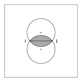
$\beta=1$
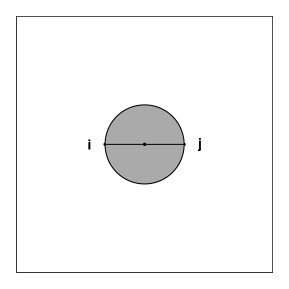
$1<\beta<2$
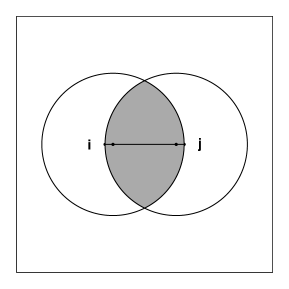
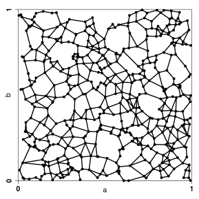
$\beta=2$

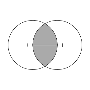
Fig. 1: Illustration of the construction of $\beta$-skeletons in a unit square for different values of $\beta$, where the region $R$ is shaded gray, with an example with $n=500$ nodes for each. From top to bottom: $\beta=0.8,1.0,1.8,2.0$.

2.1 Generalization of $\beta$-skeleton graphs

The generalization of the $\beta$-skeleton graphs is constructed by considering a rectangle $[0,a]\times[0,b]$ where $a,b\in\mathbb{R},\ a\geq b$. Only unit rectangles of the form $[0,a]\times[0,a^{-1}]$ will be considered here. The rest of the construction of a rectangular $\beta$-skeleton graph is similar to that of a $\beta$-skeleton graph. That is, $n$ points are distributed uniformly and independently in the unit rectangle $[0,a]\times[0,a^{-1}]$. Obviously, when $a=1$ the rectangle $[0,a]\times[0,a^{-1}]$ is simply the unit square $[0,1]^{2}$, which means that the rectangular $\beta$-skeleton graph becomes the classical $\beta$-skeleton one.

Figure 2 illustrates two rectangular $\beta$-skeleton graphs with $\beta=2$ and different values of the rectangle side length $a$ and the same number of nodes. In the first case when $a=1$ the graph corresponds to the classical $\beta$-skeleton graph in which the nodes are embedded into a unit square. The second case corresponds to $a=2$ which is a slightly elongated rectangle.

Fig. 2: Example RNGs for $a=1$ (top) and $a=2$ (bottom), with $n=1686$ nodes which corresponds to a particular RFN.

3 Structural characterization of networks

One of the goals of this paper is to make a comparison between real-world fracture networks and the random rectangular neighborhood networks for different values of the rectangle elongation parameter. This similarity analysis is carried out by considering a structural characterization of both types of networks using a series of network-theoretic parameters. In this section these parameters are defined along with appropriate references for the reader to dip into their general characteristics. All these parameters are based on the main matrix representations of graphs, which are the adjacency $A=\left[A_{ij}\right]_{n\times n}$, the Laplacian $\mathcal{L}=\left[\mathcal{L}_{ij}\right]_{n\times n}$ and the normalized Laplacian $\hat{\mathcal{L}}=\left[\hat{\mathcal{L}}_{ij}\right]_{n\times n}$ matrices, which are defined respectively as follows:

$A_{ij}=\left\{\begin{array}[]{c}1\\ 0\end{array}\right.\begin{array}[]{c}\textnormal{if }\left(i,j\right)\in E\\ \textnormal{otherwise}\end{array}\quad\mathcal{L}_{ij}=\left\{\begin{array}[]{c}-1\\ k_{i}\\ 0\end{array}\right.\begin{array}[]{c}\textnormal{if }\left(i,j\right)\in E\\ \textnormal{if }i=j\\ \textnormal{otherwise}\end{array}\quad\hat{\mathcal{L}}_{ij}=\left\{\begin{array}[]{c}-\sqrt{k_{i}k_{j}}\\ 1\\ 0\end{array}\right.\begin{array}[]{c}\textnormal{if }\left(i,j\right)\in E\\ \textnormal{if }i=j\\ \textnormal{otherwise}\end{array}$

There is also the distance matrix $D=\left[d_{ij}\right]_{n\times n}$, where $d_{ij}$ is the number of edges in the shortest path connecting $i$ and $j$. The definition of the structural parameters used in this work are given in Table 1. For the indices of general use see Estrada (2011) where the indices are explained.

Table 1: Structural parameters used in this work

No.	Index	Formula	Observations	Ref.
1	Average degree	$$\bar{k}=\dfrac{2m}{n}$$	$m$ is the number of edges in the graph.	Estrada (2011)
2	Largest eigenvalue of $A$	$$\lambda_{1}$$	$\lambda_{1}>\lambda_{2}\geq\cdots\geq\lambda_{n}$, it represents a sort of average degree in the network.	Estrada (2011)
3	Degree variance	$$V=\dfrac{1}{n}\sum_{i=1}^{n}\left(k_{i}-\bar{k}\right)^{2}$$	A measure of degree irregularity in a graph.	Snijders (1981)
4	Collatz-Sinogowitz index	$$\lambda_{1}-\bar{k}$$	A measure of degree irregularity in a graph.	Von Collatz and Sinogowitz (1957)
5	Degree heterogeneity	$\rho=\sum_{i,j}\hat{\mathcal{L}}_{ij}$	A measure of degree irregularity in a graph.	Estrada (2010)
6	Degree assortativity	$r$	Pearson correlation coefficient of the degree-degree correlation. $r>0$ (degree assortativity) indicates a tendency of high degree nodes to connect to other high degree ones. $r<0$ (degree disassortativity) indicates the tendency of high degree nodes to be connected to low degree ones.	Newman (2002)
7	Clustering coefficient	$$\bar{C}=\dfrac{1}{n}\sum_{i=1}^{n}\dfrac{2t_{i}}{k_{i}\left(k_{i}-1\right)}$$	$t_{i}$ is the number of triangles incident to the vertex $i:$ $t_{i}=\dfrac{1}{2}\left(A^{3}\right)_{ii}$	Watts and Strogatz (1998)
8	Diameter	$$d=\max d\left(i,j\right)$$	The largest entry of the distance matrix $D$.	Estrada (2011)
9	Average path length	$$\bar{l}=\dfrac{1}{n\left(n-1\right)}\sum_{i<j}d\left(i,j\right)$$	A measure of the ‘small-worldness’ of the network.	Estrada (2011)
10	Spectral gap	$$\varDelta=\lambda_{1}-\lambda_{2}$$	A quantity related to isoperimetric properties of graphs. A large spectral gap indicates the lack of structural bottlenecks in the network.	Estrada (2011)
11	Largest eigenvalue of $\mathcal{L}$	$$\mu_{n}$$	$$0=\mu_{1}<\mu{}_{2}\leq\cdots\leq\mu_{n}$$	Estrada (2011)
12	Algebraic connectivity	$$\mu_{2}$$	A measure of the connectivity of the graph.	Fiedler (1973)
13	Estrada index	$$EE=\sum_{j=1}^{n}G_{pp}$$	$G_{pp}=\sum_{j=1}^{n}\varphi_{j,p}^{2}\exp\left(\lambda_{j}\right)$ is a centrality measure quantifying the participation of the node $p$ is subgraphs of the graph, giving more weight to the smaller ones.	Estrada (2000)
14	Spectral bipartivity	$$b_{s}=\dfrac{\sum_{j=1}^{n}\cosh\left(\lambda_{j}\right)}{\sum_{j=1}^{n}\exp\left(\lambda_{j}\right)}$$	$0<b_{s}\leq 1,$ with the lower bound obtained for the complete graph $K_{n}$ when $n\rightarrow\infty$ and the upper bound obtained for any bipartite graph.	Estrada and Rodríguez-Velázquez (2005)
15	Average communicability distance	$$\bar{\xi}=\dfrac{\sum_{p<q}\left(G_{pp}+G_{qq}-2G_{pq}\right)^{1/2}}{n\left(n-1\right)}$$	A measure of the average quality of communication in a network, where $G_{pq}=\sum_{j=1}^{n}\varphi_{j,p}\varphi_{j,q}\exp\left(\lambda_{j}\right)$ is the communicability between the corresponding nodes.	Estrada (2012a)
16	Average communicability angle	$$\bar{\theta}=\dfrac{\sum_{p<q}\cos^{-1}\left(\dfrac{G_{pq}}{\sqrt{G_{pp}G_{qq}}}\right)}{n\left(n-1\right)}$$	A measure of spatial efficiency of a network. $0\leq\bar{\theta}\leq 90$, where the lower bound indicates high spatial efficiency and the upper one indicates a poor spatial efficiency.	Estrada and Hatano (2014)
17	Entropy	$S=-\sum_{j=1}^{n}p_{j}\ln p_{j}$	A measure of the information content of the spectrum of the adjacency matrix, where $p_{j}=\dfrac{\exp\left(\lambda_{j}\right)}{EE}$	Estrada and Hatano (2007)
18	Free energy	$F=-\ln EE$	A measure of network robustness.	Estrada and Hatano (2007)
19	Kirchhoff index (resistance distance)	$Kf=\sum_{i<j}\varrho_{ij}$	A measure related to hitting and commute times in a random walk on the network, where $\varrho_{ij}=\sum_{k=2}^{n}\dfrac{1}{\mu_{k}}$ $\left(\psi_{k,i}-\psi_{k,j}\right)^{2}$	Klein and Randíc (1993)

The number of 18 small subgraphs are also calculated, labeled as indices 20-37. The formulae for them are found in Estrada (2011) and a Matlab code for their calculation is provided in Appendix B of this work.

4 Properties of RRNGs

Here we show how some of the properties of the RRNG change with the elongation parameter, to show why the model can be of practical interest. We focus on just a few of the most important structural parameters here: the average node degree, the diameter, and the algebraic connectivity $\mu_{2}$. First we prove the following result about the diameter of the RRNG.

Lemma 1

Let $G=G\left(n,a,\beta=2\right)$ be a connected RRNG with $n$ nodes embedded in a rectangle of sides with lengths $a$ and $b=a^{-1}$. Let $D=D\left(G\right)$ be the diameter of the corresponding RRNG. Then,

$$D\left(G\right)\geq\dfrac{\sqrt{\left(a^{4}+1\right)n}}{a}.$$ (1)

Proof

The nodes of the RRNG are uniformly and independently distributed in the unit rectangle. Then, let us assume that the $n$ points are equally spaced in the area of the rectangle separated by a Euclidean distance $L$. In this case the largest number of points are connected along the main diagonal of the rectangle. If the length of the main diagonal is $c$ there are $\dfrac{c}{L}$ connected nodes in this line. Thus, the maximum shortest path distance in the RRNG is $\dfrac{c}{L}$ with $c=\dfrac{\sqrt{a^{4}+1}}{a}$. For a connected RNG this is the shortest the diameter can be, because if two points in the main diagonal are separated at a Euclidean distance larger than $L$, then the diameter of $G$ will be larger than $\dfrac{c}{L}$. Now, the main problem here is to determine the value of $L$ for the separation of two points in the RRNG. Here we consider that the $n$ points can be distributed in the square ($a=1$) forming a regular square lattice. In this case there should be $\sqrt{n}$ rows of $\sqrt{n}$ points equally spaced in the square. Thus, the separation between two points is $L=1/\sqrt{n}$. In the case of the rectangle we follow a naive approach of considering that a rectangle of major length $a>1$ can be obtained just by cutting the square $a$ times in the direction of the $y$-axis and pasting the cut rectangle along the $x$-axis. In this way it is guarantee that the separation between two points in the original square remains the same in the elongated rectangle. That is, $L=1/\sqrt{n}$ for any value of $a$, such that we have the final result. ∎

Obviously, we can fit the values of the right-hand-side of (1) to the actual values of the diameter in RRNGs of different sizes. That is, we can obtain an empirical relation of the kind $D\left(G\right)\approx c\dfrac{\sqrt{\left(a^{4}+1\right)n}}{a},$ where $c$ is a fitting parameter. By doing so for RRNGs with sizes $n=500,...,1000$ we found that $c\approx 1.414$ and the correlation coefficient between the observed and the calculated diameter is larger than 0.999 (see the plot in Figure 3).

The previous results is very important because it allow us to bound the algebraic connectivity of the RRNG. The algebraic connectivity–as we will see later on this paper–is a fundamental parameter for understanding the diffusive processes taking place on RRNGs. Then, we prove here the following result.

Lemma 2

Let $G=G\left(n,a,\beta=2\right)$ be a connected RRNG with $n$ nodes embedded in a rectangle of sides with lengths $a$ and $b=a^{-1}$. Let $k_{max}$ be the maximum degree of any node in $G$. Then, the second smallest eigenvalue of the Laplacian matrix of the RRNG is bounded as

$$\mu_{2}\left(G\right)\leq\dfrac{8k_{max}a^{2}}{a^{4}+1}\dfrac{\log_{2}^{2}n}{n},$$ (2)

Proof

We simply substitute our bound for the diameter of the RRGN into the Alon-Milman bound for the algebraic connectivity of any graph 3,

$$\mu_{2}\left(G\right)\leq\dfrac{8k_{max}}{D^{2}}\log_{2}^{2}n.$$ (3)

∎

It should be noticed that in RRNGs the value of $k_{max}$ is typically quite small. In all our simulations it is not bigger than $6$. These two theoretical results clearly indicate that the properties of the RRNG are significantly and non-trivially affected by the elongation of the rectangle. The diameter of the RRNGs increases almost linearly with the elongation of the rectangle. On the other hand, the elongation of the rectangle in the RRNG makes the graphs drastically less connected. In order to see these effects in practice we develop a series of simulations considering RRNGs with $n=1000$ nodes, $1\leq a\leq 5$ in steps of $0.5$, which we find to be a sufficiently large range of elongations for the analyses in this work. It is clear that in the limit as $a\rightarrow\infty$ the RRNG tends to the path graph $P_{n}$, which will dictate the behavior at larger elongations not seen in these plots, except for the average node degree to demonstrate this behavior. As the elongation increases, the average node degree decreases since the perimeter increases and nodes near the boundary are surrounded by fewer nodes to attach to; with further elongation the value will approach $\bar{k}=2-2/n\simeq 2$. As predicted by our theoretical results, the diameter of the RRNGs increases almost linearly with the elongation of the rectangle and the algebraic connectivity decay in a nonlinear fashion with it. Therefore, we conclude that as the elongation of the RRNG model is increased, the structural parameters also change, including those closely connected to dynamical processes such as the algebraic connectivity.

Fig. 3: Plots of how several structural parameters of the RRNG model changes as the elongation of the rectangle varies from $a=1$ to $a=5$ for $n=1,000$ nodes: (a) average node degree, (b) diameter, (c) $\mu_{2}$.

5 Rock Fracture Networks

This section describes the dataset of real-world networks consisting of the channels and their intersections produced by fractures in rocks of petrophysical interest. The procedures described hereafter are based on the analysis developed by Santiago et al. (2013). These authors have considered a series of rocks extracted from wells in the Gulf of Mexico. The rocks are cut into two halves and images are taken of one of the rock halves, which show the fractures in the corresponding rock. An algorithm is then used to find the skeleton of these fractures and construct a network representation of it, which is stored as an adjacency matrix. The nodes of the network correspond to where fractures intersect or terminate and an edge between nodes corresponds to a channel between those points in the skeleton of the rock fracture. A sketch of the process is illustrated in Fig. 4.

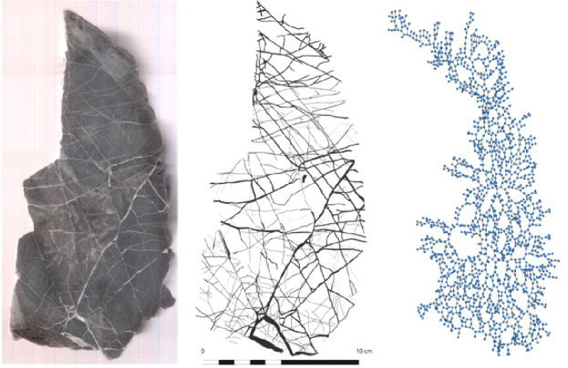
Fig. 4: Illustration of the process of creating rock fracture networks from rock samples. (Left) A rock sample from the Gulf of Mexico showing one of the halves of the rock. (center) Digital image of the rock illustrating the fractures existing in it. (right) Rock fracture network created from the digital image by taking the intersection of channels as the nodes and channels as the edges of the network. Image is courtesy of E. Santiago.

In total 29 rock samples are considered here, kindly provided by Santiago et al. (2013, 2016, 2014). The number of nodes $n$ and edges $m$ in the 29 networks studied here are provided in Table (2) together with the labels used in the subsequent analysis in this work.

No.	$n$	$m$	$a$		No.	$n$	$m$	$a$
M1	93	109	$1.0$		M16	779	887	$1.5$
M2	46	54	$1.5$		M17	633	728	$1.5$
M3	71	74	$2.0$		M18	3585	4183	$1.5$
M4	109	124	$1.5$		M19	97	101	$2.0$
M5	346	380	$3.5$		M20	1567	1996	$1.0$
M6	85	89	$2.5$		M21	70	74	$2.0$
M7	55	60	$1.0$		M22	1686	1905	$2.0$
M8	87	94	$1.0$		M23	396	396	$4.5$
M9	44	46	$1.0$		M24	181	180	$5.0$
M10	296	336	$1.5$		M25	394	418	$4.0$
M11	47	48	$2.0$		M26	808	813	$4.5$
M12	46	47	$1.5$		M27	223	222	$4.0$
M13	215	233	$2.5$		M28	297	305	$4.0$
M14	132	144	$1.5$		M29	363	365	$5.0$
M15	40	40	$2.0$

Table 2: Rock fracture networks studied in this work, their number of nodes $n$, and number of edges $m$.

6 Similarity between Fracture Networks and RNGs

This section aims to compare the real-world rock fracture networks with their random analogues created by using the $\beta$-skeleton approach. To achieve this goal random rectangular neighborhood graphs are created with a value of $\beta=2$ and having the same number of nodes and edges as the corresponding real-world fracture network. The elongations of the rectangle are varied in the range $1\leq a\leq 5$ with a step $0.5$. The selection of the value $\beta=2$ in this study is based on empirical observations of the dataset of rock fracture networks under analysis. First, these real-world networks are always planar and have a relatively low number of triangles. These two characteristics are well-reproduced by the relative neighborhood graphs corresponding to $\beta=2$. Furthermore, these RNGs have been widely considered in the literature and can be constructed more easily and quickly then an a $\beta$-skeleton for some arbitrary value of $\beta$.

Then, for each graph, a $k\times 1$ vector is calculated consisting of the $k$ structural properties defined previously (including the 18 small subgraphs). That is, every network is represented in a $k$-dimensional space ($k=37)$ in which each coordinate represents a structural parameter, e.g., average degree, clustering coefficient, etc. A number of random constructions are realized of the RRNG for each elongation and the value averaged over all of them. The number of random realizations varies depending on the size of the network for reasons of computational difficulty, with effort made to ensure a large enough number of realizations such that the variance is not too large.

The similarity between the real-world rock fracture networks and their RRNG analogues can then be calculated, we may also refer to the dissimilarity which is simply a different view of the same quantity. This similarity is quantified by simply using the Euclidean distance between the corresponding points in the $k$-dimensional property space in which they are represented, and thus the similarity may referred to as the “distance” when convenient. A potential problem arising here is the fact that the values of the properties calculated lie in a very wide range of numerical values. Then, the values of each property are normalized to lie in the range between 0 and 1. Such normalization is carried out as follows. Let $r_{i,0}$ be the property vector for the $i$th RFN, and $r_{i,j}$ be the property vector for the RRNG analogous of the corresponding RFN created with the $j$th elongation $a$ of the rectangle, $1\leq j\leq 9$, and for each elongation this is averaged over all random realizations to obtain a single vector for each. Each vector $r_{i,j}$ is then normalized as follows for $0\leq j\leq 9$

$$\hat{r}_{i,j}(p)=\dfrac{r_{i,j}\left(p\right)-\min_{j}r_{i,j}\left(p\right)}{\max_{j}r_{i,j}\left(p\right)-\min_{j}r_{i,j}\left(p\right)},$$ (4)

where $r_{i,j}\left(p\right)$ represents the $p$th entry of the $r_{i,j}$ vector. That is, for a given RFN and property, the value of this property is normalized for the RFN and all corresponding elongations of RRNG so that they lie between 0 and 1, with the smallest value mapped to 0 and the largest mapped to 1.

It is observed that for each of the rock fracture networks there is a minimum in the plot of the dissimilarity versus the rectangle elongation (see Fig. 5(a)), which indicates that there is an optimal elongation for each RRNG that makes it most similar to the real-world fracture network. In Fig. 5(b), the frequency with which the maximum similarity occurs for a given value of the rectangle elongation $a$ is plotted. It can be seen that the histogram is two-peaked with the first maximum corresponding to elongations between $a=1$ and $a=2$ and the second one for elongations around $a=4$. The first peak clearly corresponds to rock fracture networks that are better reproduced by almost square neighborhood graphs. However, the second group of real-world fracture networks are better reproduced by elongated rectangles in which one of the sides of the rectangle is about 16 times longer than the other. A more detailed statistical analysis of the histogram of the optimal elongations shows that the modal value of elongation is $a=1.5$, and elongations between $a=1$ and $a=2$ are the most common, accounting for about $2/3$ of the rocks. The rest of the values lie between $a=2.5$ and $a=4.5$, except for a couple of rocks which have minimum at $a=5.$

The most interesting observation carried out in this analysis is the following. Most of the rock fracture networks which are better reproduced by almost square RRNGs correspond to the smallest ones, while those which are better reproduced by elongated RRNGs are those having the largest number of nodes. These results are illustrated in Fig. 5(c and d) where the networks are split into two groups, those with $n\leq 150$, and those with $n>150$. As can be seen in Fig. 5(c), which corresponds to the first group, the maximum similarity occurs for $1\leq a\leq 2$. However, for the largest networks the maximum similarity occurs for values of $3\leq a\leq 4$. In closing, the rock fracture networks are better described by the RRNGs depending on the size of the networks, with almost square RRNG describing better the smallest RFNs and more elongated RRNGs describing better the largest RFNs. In other words, it is more plausible that larger RFNs are those coming from elongated rocks and consequently better reproduced by RRNGs with $a>1$ which better reproduce this characteristic. The smallest RFNs appear to come from more rounded rocks, which are better reproduced by almost-square RRNGs.

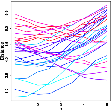
Fig. 5: (a) Variation of the dissimilarity between RFNs and the corresponding RRNGs for different values of the rectangular elongation $a$. Each curve corresponds to one pair RFN-RRNG. (b) Number of graphs for which the minimum dissimilarity appears at a given value of the rectangle elongation $a$. (c) Average variation of the dissimilarity between RFNs and the corresponding RRNGs for different values of the rectangular elongation $a$ for RFNs with less than 150 nodes. The vertical bars represent the standard deviation. (d) Average variation of the dissimilarity between RFNs and the corresponding RRNGs for different values of the rectangular elongation $a$ for RFNs with more than 150 nodes. The vertical bars represent the standard deviation.

The RRNGs reproduce relatively well the main structural properties of real-world RFNs of different sizes. This conclusion is reached by the fact that the dissimilarity between the RFNs and the RRNGs is generally smaller than the dissimilarity between the RFNs and other commonly used random graph models. A comparison is made here between the use of the RRNGs and the Erdős–Rényi (ER), Barabási–Albert (BA), and random rectangular graph (RRG) models. The ER graphs $G\left(n,p\right)$ are created from a set of $n$ nodes which are randomly picked in pairs and connected with certain probability $p$. In the BA model a graph $G\left(n,m_{0}\right)$ is created on the basis of a seed of $n_{0}$ nodes which are connected randomly and independently according to an ER model. Then, new nodes are added one at a time and connected to $m_{0}$ of the existing nodes in the graph with a probability that depends on the degree of the nodes. Then, instead of obtaining a Poisson distribution of the node degree as in the ER model, the model ends up with a power-law degree distribution. Finally, the RRG $G\left(n,a,r\right)$ is created from $n$ points randomly and independently distributed on the unit rectangle of sides $a$ and $1/a$. Then, a disk of radius $r$ is centered on a point $i$, and every node inside that disk is connected to $i$. The process is repeated for each of the $n$ points. Notice that all the random graphs must be connected in order to calculate some of the structural parameters. For the ER model the value of $p=\log n/n$ was chosen, which is the critical value at which the large connected component appears, with discarding of any random realizations in which the networks were disconnected. For the RRG model, again elongations from $a=1$ to $a=5$ in steps of $0.5$ were used, and the best elongations were selected for each rock individually in exactly the same manner as for the RRNG model. In every case, the radius $r$ was selected to ensure the RRG was connected with high probability, since selecting $r$ to best match the number of edges in the RFN would almost always give a disconnected graph. In each case, several random realizations were taken and the results averaged, with fewer realizations used in the case of a large number of nodes for reasons of computational difficulty.

With this data, the models were compared to see which of them works the best. Let $r_{i,0}$ be the property vector for the $i$th RFN, and $r_{i,j}$ be the property vector for the $j$th model, $1\leq j\leq 4$, where for the RRNG and the RRG only the best elongation is used. Then, the normalization takes exactly the same form as Eq. 4. After this normalization, dissimilarities between the RFNs and each model were calculated. As can be seen in Fig. 6(a) the RRG model is the worst, with a dissimilarity larger than 5 for all RFNs, which is more than double the largest dissimilarity for any other model. To better compare the remaining models, the RRG model was removed from the analysis and the dissimilarities were recomputed with the remaining three models, since the presence of the data from the RRG model affects the normalization values. The results are illustrated in Fig. 6(b) where it can be noted that the ER model is much worse than the other two, so this model was also removed. The result is the comparison of the best two models, the RRNG and the BA, which is illustrated in Fig. 6(c). In the large majority of cases the RRNG is observed to be the best model to reproduce the topological properties of the rock fracture networks due to a smaller value of dissimilarity.

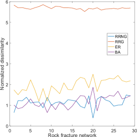
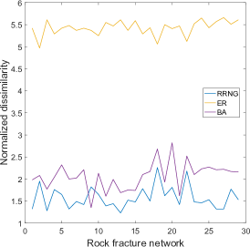
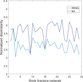
Fig. 6: Relative normalized dissimilarity (the dissimilarity after the data has been normalized as described in the main text) between the RFNs and four theoretical models: random rectangular neighborhood networks (RRNG), random rectangular graphs (RRG), Erdős-Rényi (ER) and Barabási-Albert (BA). From left to right the iterative process described in the main text is shown where the least similar model is eliminated until the two best models remain.

7 Fluid diffusion on fracture networks and on RRNGs

In this section a diffusion process is modeled as occurring through the channels of rock fracture networks. The flow of fluids through porous media is frequently described by the Boussinesq equation (also known as the porous media equation):

$$\dfrac{\partial}{\partial t}u\left(x,t\right) = \dfrac{\partial}{\partial x}\left(u\left(x,t\right)\dfrac{\partial}{\partial x}u\left(x,t\right)\right),$$ (5)

$$u\left(x,0\right) = u_{0}$$ (6)

where $u\left(x,t\right)$ is a non-negative scalar function on $x\in\Omega=\left[0,1\right]\subset\mathbb{R}$ and time $t\in\mathbb{R}\geq 0$.

Suppose that the fluid is flowing through a capillary of length $L$ and height $h_{0}$, and suppose that the capillary is much longer than it is thick: $L\gg h_{0}.$ Then, according to Hasan et al. (2012) (see especially Fig. 4) and Polubarinova-Kochina (1962), the Boussinesq equation can be very well approximated by a simple heat equation

$$\dfrac{\partial}{\partial t}u\left(x,t\right) = \dfrac{\partial^{2}}{\partial x^{2}}u\left(x,t\right),$$ (7)

$$u\left(x,0\right) = u_{0}.$$ (8)

Obviously, the channels produced by the fractures of rocks are less than a millimeter thick and a few centimeters long. Thus, $L\gg h_{0}$ is always true and the use of the heat equation is justified for modeling the diffusion of oil and gas through the channels formed by the network of rock fractures. In the case of diffusion through the edges of a network the previous equation can be written as

$$\dfrac{\partial}{\partial t}u\left(x,t\right) = -\mathcal{L}u\left(x,t\right),$$ (9)

$$u\left(x,0\right) = u_{0},$$ (10)

where $\mathcal{L}$ is the graph Laplacian defined previously in this work.

In order to select the initial condition vector $u_{0}$ two different scenarios are considered. The first one considers the case in which only a few nodes of the rock fracture network are in contact with the reservoir as illustrated in Fig. 7(a). This initial condition is used mainly to study the influence of the flow directionality on the diffusion through the rock fracture network and will be referred to as directional diffusion. In this case the vector $u_{0}$ is constructed such that the entry $u_{0}\left(i\right)$ is a random number for those nodes considered to be in contact with the reservoir, which are randomly selected from the set of nodes of the graph and should have the condition that they are close in space to each other. This set of points is selected from one of the two extremes of the longest path (diameter) of the graph. The rest of the entries of the initial condition vector are set to zero. The second scenario is based on the assumption that the RFN is in contact with the reservoir from many different positions as illustrated in Fig. 7(b), and will be called anisotropic diffusion. In this case the entries $u_{0}\left(i\right)$ of the initial condition vector are selected randomly for each of the nodes of the graph. The results of these two types of initial conditions are highly correlated, with a Pearson correlation coefficient of 0.999. The directional diffusion takes longer, since the oil must spread along the diameter of the rock from one end in this case, whereas in the anisotropic case there is already oil spread (unevenly) throughout the rock at time $t=0$. On average, the directional diffusion takes $1.44$ times longer than the anisotropic one. Due to these similarities, hereafter only the case where the whole rock is in contact with the reservoir is considered (Fig. 7(b)).

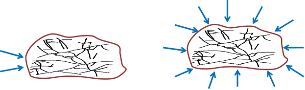
Fig. 7: Illustration of the two scenarios used for modeling the diffusion of oil and gas from a reservoir through the fracture network of a rock. (a) Only a small region of the rock is in contact with the reservoir. (b) The whole rock is in contact with the reservoir.

It is considered that the diffusion process has taken place if $|u\left(i,t\right)-u\left(j,t\right)|\leq\delta$ for all pairs of nodes $i$ and $j$ in the graph when $t\rightarrow\infty$. In this work a threshold of $\delta=10^{-5}$ is selected. This means that if the “concentration” of the diffusive particle in one node does not differ from that in any other node by more than $\delta=10^{-5}$ it is considered that the diffusion process has ended. Then, the time at which this threshold is reached is recorded, and is called the diffusion time. Due to the fact that many realizations of the same process are carried out the average of this time is taken over all these realizations. Once the values of the average time of diffusion are obtained for each RFN, correlations are obtained with the structural parameters considered in this work in order to see which of them influence the diffusive process on the RFNs. Table 3 reports the Pearson correlation coefficients of these relations, where the entries in boldface are those that are more significant from a statistical point of view. The next subsection will analyze the theoretical foundations for these findings.

structural parameter	correlation	log		structural parameter	correlation	log
1	0.026			$F_{1}$	0.815	Y
3	-0.307			$F_{2}$	0.415
4	0.225			$F_{3}$	0.775	Y
5	-0.613			$F_{4}$	0.764	Y
6	0.142			$F_{5}$	0.423
7	-0.127			$F_{6}$	0.418
8	0.809	Y		$F_{7}$	0.387
9	0.745	Y		$F_{8}$	0.419
10	-0.495	Y		$F_{9}$	0.435
11	0.449			$F_{10}$	0.416
12	-0.995	Y		$F_{11}$	0.409
13	0.841	Y		$F_{12}$	0.381
14	0.104			$F_{13}$	0.424
15	0.328			$F_{14}$	0.389
16	0.872			$F_{15}$	0.407
17	0.876			$F_{16}$	0.000
18	-0.845			$F_{17}$	0.412
19	0.923	Y

Table 3: Results of the regression analysis between the diffusion time in RFNs and structural parameters of the same networks. The numerical values correspond to the Pearson correlation coefficient and “log” indicates whether the correlation is in a log-log scale. The numbers used for the structural parameters are given in Table 1 and the structure of the fragments is given in Appendix A.

Figure 8 illustrates the correlation between the average diffusion time obtained by simulation of the diffusive process on the RFNs versus the same process simulated on the analogous RRNGs. In addition, it provides evidence that the average diffusion time simulated on the RFNs is correlated to some of the most important structural parameters of the RRNGs. This means that the real-world RFNs can be replaced by their analogous random models in order to simulate the diffusion processes taking place on the rocks.

Fig. 8: (a) Plot of the average diffusion time of the RFNs versus the diffusion time in the analogous RRNGs. Plot of the diffusion time of the RFNs versus algebraic connectivity (b), resistance distance (Kirchhoff index) (c) and average communicability angle (d) in the analogous RRNGs.

7.1 Theoretical analysis

As can be seen in Table (3) the best structural parameter describing the diffusion time is the second smallest eigenvalue of the Laplacian matrix, $\mu_{2}$. In order to understand this relation, consider the solution of the diffusion equation (Eq. 9), which is:

$$\vec{u}\left(t\right)=e^{-t\mathcal{L}}\vec{z},$$ (11)

where $\vec{z}=\vec{u}_{0}$. In terms of the spectral decomposition of the graph Laplacian, the solution of the diffusion equation (Eq. 9) can be written as

$$\vec{u\left(t\right)}=e^{-t\mu_{1}}\left(\vec{\psi}_{1}\cdot\vec{z}\right)\vec{\psi}_{1}+e^{-t\mu_{2}}\left(\vec{\psi}_{2}\cdot\vec{z}\right)\vec{\psi}_{2}+\cdots+e^{-t\mu_{n}}\left(\vec{\psi}_{n}\cdot\vec{z}\right)\vec{\psi}_{n},$$ (12)

where $0=\mu_{1}<\mu_{2}\leq\cdots\leq\mu_{n}$ are the eigenvalues and $\vec{\psi}_{j,p}$ the $p$th entry of the corresponding $j$th eigenvector of the Laplacian matrix, and $\vec{x}\cdot\vec{y}$ represents the inner product of the corresponding vectors. Equation 12 can be written for a given node $p$ as

$$\vec{u}_{p}\left(t\right)=\sum_{q=1}^{n}\vec{z}_{q}\sum_{j=1}^{n}\vec{\psi}_{j,p}\vec{\psi}_{j,q}e^{-t\mu_{j}},$$ (13)

which represents the evolution of the state of the corresponding node as time evolves. Now, consider that the time tends to the time of diffusion $t\rightarrow t_{c}$, where $t_{c}$ is the time at which $|u_{i}(t)-u_{j}(t)|\leq\delta$ for all $i,j$. Denote this time by $t_{c}^{-}$, and then

$$\vec{u}_{p}\left(t_{c}^{-}\right)=\frac{1}{n}\sum_{q=1}^{n}\vec{z}_{q}+\sum_{j=2}^{n}\left(\vec{\psi}_{j,p}e^{-t_{c}^{-}\left(p\right)\mu_{j}}\sum_{q=1}^{n}\vec{\psi}_{j,q}\vec{z}_{q}\right),$$ (14)

where here $t_{c}^{-}\left(p\right)$ means the time at which the node $p$ is close to reaching the diffusion state. Let $\left\langle\vec{u}_{0}\right\rangle=\frac{1}{n}\sum_{q=1}^{n}\vec{z}_{q}$ and write Eq. 14 as follows

$$\vec{u}_{p}\left(t_{c}^{-}\right)-\left\langle\vec{z}\right\rangle=\sum_{j=2}^{n}\left(\vec{\psi}_{j,p}e^{-t_{c}^{-}\left(p\right)\mu_{j}}\sum_{q=1}^{n}\vec{\psi}_{j,q}\vec{z}_{q}\right).$$ (15)

A node $p$ is selected such that $\vec{\psi}_{2,p}$ has the same sign as $\vec{\psi}_{2}\cdot\vec{z}$. Since $\mu_{2}$ is the smallest eigenvalue in the sum on the right hand of the expression, this terms tends to 0 slower than the terms for the other values of $j$. This means that, if $\delta$ is sufficiently small, the values of $t_{c}$ and thus $t_{c}^{-}$ will be very large. Thus, it is possible to ensure that the left side of the equation is small enough such that $\sum\limits_{j=3}^{n}\left(\vec{\psi_{j,p}}e^{-t_{c}^{-}(p)\mu_{j}}(\vec{\psi_{j}}\cdot\vec{z})\right)<0$. This implies that

$$\left(\vec{u}_{p}\left(t_{c}^{-}\right)-\left\langle\vec{z}\right\rangle\right)<\vec{\psi}_{2,p}e^{-t_{c}^{-}\left(p\right)\mu_{2}}\left(\vec{\psi}_{2}\cdot\vec{z}\right).$$ (16)

Now, because $\left|\vec{u}_{p}\left(t_{c}^{-}\right)-\left\langle\vec{z}\right\rangle\right|\geq\delta$,

$$\delta\leq\left|\vec{u}_{p}\left(t_{c}^{-}\right)-\left\langle\vec{z}\right\rangle\right|<\left|\vec{\psi}_{2,p}e^{-t_{c}^{-}\left(p\right)\mu_{2}}\left(\vec{\psi}_{2}\cdot\vec{z}\right)\right|.$$ (17)

Then, the time at which the diffusion is reached $t_{c}\left(p\right)$ is bounded by

$$t_{c}\left(p\right) \geq t_{c}^{-}\left(p\right)\geq\frac{1}{\mu_{2}} \ln\left|\frac{\vec{\psi}_{2,p}\left(\vec{\psi}_{2}\cdot\vec{z}\right)}{\delta}\right|.$$ (18)

Finally, the average time of diffusion is bounded by

$$\left\langle t_{c}\right\rangle\geq\frac{1}{\mu_{2}n}\sum_{p=1}^{n}\ln\left|\frac{\vec{\psi}_{2,p}\left(\vec{\psi}_{2}\cdot\vec{z}\right)}{\delta}\right|.$$ (19)

As can be seen from Eq. 19 the average diffusion time in a network inversely correlates with the second smallest eigenvalue of the Laplacian matrix (see also the negative Pearson correlation coefficient in Table 3). This analysis clearly indicates that $\mu_{2}$ can be used as an estimator of the rate of diffusion of oil and gas in rock fracture networks. Using our previous results in which we found a bound for the diameter and for the algebraic connectivity of RRNGs we can easily prove the following one.

Lemma 3

Let $G=G\left(n,a,\beta=2\right)$ be a connected RRNG with $n$ nodes embedded in a rectangle of sides with lengths $a$ and $b=a^{-1}$. Let $k_{max}$ be the maximum degree of any node in $G$. Then, the second smallest eigenvalue of the Laplacian matrix of the RRNG is bounded as

$$\left\langle t_{c}\right\rangle\geq\left(\frac{a^{4}+1}{8k_{max}}\dfrac{1}{\log_{2}^{2}n}\right)\sum_{p=1}^{n}\ln\left|\frac{\vec{\psi}_{2,p}\left(\vec{\psi}_{2}\cdot\vec{z}\right)}{\delta}\right|.$$ (20)

This result clearly explains why the diffusion time correlates relatively well with the diameter of the graph. That is, as the elongation increases, the algebraic connectivity decays as a consequence of the increase of the diameter of the graph, which make the diffusion time increase. In other words, increasing the elongation of the RRNGs makes the diffusion process to take a longer time to finish.

A lower bound for the algebraic connectivity has also been reported by Mohar (1991) in terms of the average path length $\bar{l}\left(G\right)$ of the graph, which explains the correlation obtained between the diffusion time and $\bar{l}\left(G\right)$

$$\mu_{2}\left(G\right)\geq\dfrac{4}{2\left(n-1\right)\bar{l}\left(G\right)-\left(n-2\right)}.$$ (21)

On the other hand, the high correlation observed between the diffusion time and the so-called Kirchhoff index can also be understood by using the relation in Eq. 19 because the Kirchhoff index is defined by

$$Kf=\sum_{i<j}\sum_{k=2}^{n}\dfrac{1}{\mu_{k}}\left(\psi_{k,i}-\psi_{k,j}\right)^{2},$$

from which it can easily be seen that the largest contribution is made by the second smallest eigenvalue of the Laplacian matrix $\mu_{2}$ and its corresponding eigenvector (the Fiedler vector $\vec{\psi}_{2}$).

The somehow unexpected relations are those observed between the diffusion time and Estrada index, the entropy, the free energy and the average communicability angle, which are based on the adjacency instead of on the Laplacian matrix of the graph. These relations can be understood through the structural interpretation of the Estrada index in term of subgraphs of the graph. This index is defined as

$$EE\left(G\right) = tr\left(A^{0}\right)+tr\left(A\right)+\dfrac{1}{2}tr\left(A^{2}\right)+\dfrac{1}{6}tr\left(A^{3}\right)+\dfrac{1}{24}tr\left(A^{4}\right)+\dfrac{1}{120}tr\left(A^{5}\right)+\cdots.$$ (22)

Clearly, $tr\left(A^{0}\right)=n$ and $\dfrac{1}{2}tr\left(A^{2}\right)=m$ (notice that the adjacency matrix is traceless due to the lack of any self-loop in the networks). It is well-known that $\dfrac{1}{6}tr\left(A^{3}\right)=F_{2}$ is the number of triangles in the graph. In a similar way $tr\left(A^{4}\right)=2m+4F_{1}+8F_{5}$ and $tr\left(A^{5}\right)=30F_{2}+10F_{6}+10F_{8}.$ Consequently, the Estrada index of a graph can be written as

$$EE = n+\dfrac{13}{12}m+\dfrac{1}{6}F_{1}+\dfrac{5}{4}F_{2}+\dfrac{1}{3}F_{5}+\dfrac{1}{12}F_{6}+\dfrac{1}{12}F_{8}+\cdots,$$ (23)

which indicates that this index can be expressed as a weighted sum of the number of small fragments in the graph. The correlation coefficients between the diffusion time of the RFNs and their number of nodes and edges are 0.863 and 0.846, respectively. Similarly, there are high correlations with the fragments $F_{1}$, $F_{3}$, and $F_{4}$. Because the RFNs are not very dense and as previously observed they do not contain a large number of triangles (indeed there are a few RFNs which are triangle-free), this can be approximated as

$$EE \approx an+bm+cF_{1}+d,$$ (24)

where $a,b,c,d$ are coefficients. Indeed, a linear regression analysis makes an estimation of these parameters as

$$EE \approx 0.85n+0.93m+0.40F_{1}+1.56,$$ (25)

with a Pearson correlation coefficient $r>0.99999$ when including all 29 RFNs studied here. Then, it can be concluded that the correlation observed between the Estrada index and the diffusion time in RFNs is due to the fact that the diffusion time is well described by a few small fragments of the graphs, namely the number of nodes, edges and paths of length 2 ($F_{1}$), which are the main contributors to the Estrada index in these graphs. The correlations with $F_{3}$, and $F_{4}$ observed in Table (3)) can be easily explained by the fact that these fragments, in networks of poor cliquishness, are related to the fragment $F_{1}$. Finally, the relatively high correlations observed for the entropy, the free energy and the average communicability angle can be explained the fact that all of these measures are in some way related to the Estrada index of the graph (see Table 1).

8 Potential improvements of the model

8.1 Influence of fracture aperture

Any model is always a simplification of the reality made on the basis of a series of physical assumptions, empirical observations and availability of mathematical and computational tools to solve it. In this work we have used a few of these simplifications to produce a simple but effective modeling of the diffusion of fluids through rock fracture networks. However, there are a few areas in which improvements can be implemented in order to gain more realistic description of the physical processes taking place. One of our assumptions in this model is that all the fractures have the same aperture. This assumption is of course far from real, but it was used due to the lack of data about such apertures for the rock fracture networks that we studied in this work. However, such data is not difficult to obtain experimentally and we will give here some hints about how to implement this parameter and how it would affect the modeling results.

When assuming that all fracture apertures were identical we used unweighted graphs to represents the RFNs, i.e., every edge in the graph received an identical unit weight. If information concerning the aperture of the fractures were available we can represent it in our model by transforming the graphs representing RFNs into weighted graphs, in which every edge receives a weight corresponding to the aperture of that fracture. As we do not have such data for the RFNs studied here we assume that such apertures are randomly and independently distributed from $[0,1]$ over the fractures of a network. We then repeat our simulations for these weighted graphs representing RFNs with different, randomly distributed, apertures. We report here the average of the diffusion times for 10 random realizations.

In Figure 9 we show the correlation between the diffusion time in the weighted RFNs and the unweighted RFNs in a log-log scale. It is clear that there is a strong correlation between the two results, with a correlation coefficient of $0.870$. It is obvious that the diffusion times will change in dependence of the type of aperture that we use. For instance, the average times using apertures in the range $[0,1]$ is larger than that when using all weights equal to one. If apertures of larger magnitude were used, an acceleration of the diffusion process should be observed, with significantly smaller diffusion times that those observed for the unweighted case. However, what is most important here is that a power-law relation exists between the diffusion time in the unweighted and the randomly weighted networks. That is,

$$\left\langle t_{c}\right\rangle\sim\left\langle\tilde{t}_{c}\right\rangle^{\kappa},$$ (26)

where $\tilde{t}_{c}$ is the time of diffusion in the weighted RFN and $\kappa\approx 0.92$ is a fitting parameter obtained by using nonlinear regression analysis for the data displayed in Figure 9. More work is needed to show whether such kind of power-law relation exists in general between these two parameters, which would indicate some kind of universal scaling between the network with identical apertures for all the fractures and that with apertures randomly and independently distributed. In the meantime, we can assert that based on the current results knowing the behavior of diffusion on the unweighted RFNs also gives information about the behavior of the diffusion when the aperture of the fractures is randomly and independently distributed.

Fig. 9: Plot of the diffusion time for the weighted RFNs against the diffusion time with all edge weights equal to 1 (log-log scale).

8.2 Influence of long-range hops of diffusive particles

Another approximation that was considered in the current work is that the conditions of the fracture networks in terms of their homogeneity is appropriate for the use of the normal diffusion equation. However, there is currently a vast volume of literature suggesting the lack of homogeneity in many unconventional naturally fractured reservoirs of oil Albinali et al. (2016). These studies point out to the existence of complex combinations of connected and isolated pores, combinations of regions with discrete and continuous fractures and variable properties of the hydrocarbon properties across the reservoir Camacho Velazquez et al. (2012). These geological and petrophysical complexities cannot be described by using the simple diffusion equation and much more sophisticated models have emerged, which exploit the fractal nature of such irregularities. It has been well documented that such inhomogeneities in the properties of the systems to be modeled play a major role in the diffusion processes taking place, which are quite similar to anomalous diffusion in disordered media. Then, it is normal to model the geostatistics of these reservoirs by a fractional Brownian motion and fractional Lévy motion Hewett (1986); Silva et al. (2007).

Here we will follow a different path which connects in a natural way with our previous model based on the normal diffusion equation on graphs. We consider here a generalization of this equation using the so-called $d$-path Laplacian operators introduced by Estrada (2012b). In a recent work (Estrada et al. (2016)) have proved analytically the existence of anomalous diffusion—superdiffusive and ballistic behavior—when this model is used in infinite one-dimensional systems. In the case of finite graphs, Estrada et al. have shown that the biggest possible acceleration of diffusion is obtained for certain parameters of the model in any graph, independently of its topology.

Let us now define the $d$-path Laplacian matrices which account for the hopping of the diffusive particle to non-nearest-neighbors in the graph. Let $P_{l}\left(i,j\right)$ denote a shortest-path of length $l$ between $i$ and $j$. The nodes $i$ and $j$ are called the endpoints of the path $P_{l}\left(i,j\right)$. Because there could be more than one shortest path of length $l$ between the nodes $i$ and $j$ we introduce the following concept. The irreducible set of shortest paths of length $l$ in the graph is the set $P_{l}=\left\{P_{l}(i,j),P_{l}(i,r),...,P_{l}(s,t)\right\}$ in which the endpoints of every shortest-path in the set are different. Every shortest-path in this set is called an irreducible shortest-path. Let $d_{max}$ be the graph diameter, i.e., the maximum shortest path distance in the graph. Now, we have generalized the Laplacian matrix to the so-called $d$-path Laplacian matrices which are defined as follows.

Definition 1

Let $d\leq d_{max}$. The $d$-path Laplacian matrix, denoted by $\mathcal{L}_{d}\in\mathbb{R}^{n\times n}$, of a connected graph of $n$ nodes is defined as:

$$\mathcal{L}_{d}\left(i,j\right)=\left\{\begin{array}[]{r}\delta_{k}\left(i\right)\\ -1\\ 0\end{array}\right.\begin{array}[]{l}\textnormal{if $i=j$ },\\ \textnormal{if node $d_{ij}=d$ }\\ \textnormal{otherwise,}\end{array}$$ (27)

where $\delta_{k}\left(i\right)$ is the number of irreducible shortest-paths of length $d$ that are originated at node $i$, i.e., its $d$-path degree.

We can now define the generalized diffusion equation in which the $d$-path Laplacian operators are transformed by certain coefficients that make that the hopping probability of the diffusive particle decay with the distance that the particle is going to hop. Estrada et al. have analyzed mathematically three different transforms of the $d$-path Laplacian operators and proved that for the infinite linear chain there is superdiffusive behavior when the operators are transformed by using the Mellin transform with $1<s<3$. Hereafter we adopt this generalized diffusion equation which can be written in the following way:

$$\dfrac{\partial}{\partial t}u\left(x,t\right) = -\left(\sum_{d=1}^{d_{max}}d^{-s}\mathcal{L}_{d}\right)u\left(x,t\right),$$ (28)

$$u\left(x,0\right) = u_{0}.$$ (29)

Obviously, when $s\rightarrow\infty$ the terms $d^{-s}\rightarrow 0$ for all $d>1,$ and we recover the normal diffusion equation (9). In this framework we should expect just the normal diffusion to take place. However, when $s\rightarrow 0$, the system behaves as a fully-connected graph in which the diffusive particle can hop to any other node in the RFN with identical probability. For the simulations, we consider here only the case when $s=1$ and we use a stopping criterion of $\varepsilon=10^{-4}$.

We have calculated the diffusion time using the generalized diffusion equation (28) for all the RFN’s studied here and compare the generalized diffusion times with those of the normal diffusion process. The normal diffusion time averaged for all RFNs is $12,315$, while that for the generalized process is $0.69$. If we consider the ratio of both times, i.e., the diffusion time under the normal conditions $\left\langle t_{c}\right\rangle$ and the diffusion time under long range hops of the diffusive particle $\left\langle\hat{t}_{c}\right\rangle$, we see that on average it is $42,784$. It other words, the time for diffusion on the RFNs decreases 40 thousand times when we consider long-range hops. In Figure 10 we illustrate the ratio $\left\langle t_{c}\right\rangle/\left\langle\hat{t}_{c}\right\rangle$ as the effect of long-range hops for the 29 real-world fracture networks studied in this work. The most interesting thing in these results is the fact that this ratio is dramatically larger than the average for 3 of the RFNs studied. In these three cases the ratio $\left\langle t_{c}\right\rangle/\left\langle\hat{t}_{c}\right\rangle$ is ten times larger than the mean of this value for all the networks. Although this is not a signature of superdiffusion it is worth further investigation to determine whether superdiffusive behavior is observed for these three networks under the long-range hop scheme. This, however, is out of the scope of the current work and we leave it for a further and more complete investigation of this phenomena.

Another important characteristic of the results obtained in this subsection of the work is the lack of correlation between $\left\langle t_{c}\right\rangle$ and $\left\langle\hat{t}_{c}\right\rangle$ (graphic not shown). In contrast to what we have observed for the case of fracture aperture where a power-law relation was observed between the time considering random apertures and that using a fixed one, such a relation does not exist here. This lack of correlation between $\left\langle t_{c}\right\rangle$ and $\left\langle\hat{t}_{c}\right\rangle$ could be indicative of a different physical nature of the processes of diffusion under normal conditions and the diffusion under long range hops of the diffusive particle. This could show that the multi-hop approach to diffusion captures some phenomenology not captured by the normal diffusion process, which may include the case of superdiffusive behavior.

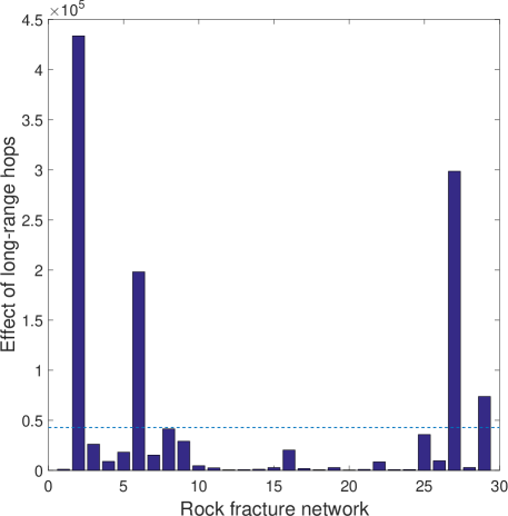
Fig. 10: Bar plot of the values of the ratio $\left\langle t_{c}\right\rangle/\left\langle\hat{t}_{c}\right\rangle$ used to account for the effect of long-range hops on the 29 real-world fracture networks studied in this work. The horizontal broken line represents the average value of this ratio for the 29 RFNs.

8.3 Influence of 3D environments

Another characteristic of the current model that can be easily incorporated to the study of diffusive processes is its extension to higher-dimensional environments. We have considered here the 2-dimensional problem only due to the fact that the data that we have represents the 2-dimensional rock slices to investigate a projection of the fracture network into a plane. However, it is obvious that such fracture networks cover the 3-dimensional space of the rock and extend over its volume.

For modeling purposes we should remark that now the number of parameters increases and that more kinds of shapes emerge. While for the case of the 2D scenario we can have only square-like or elongated rectangle-like frameworks, in 3D we have the following three main possibilities of environments: (i) a cube, (ii) an elongated cuboid, (iii) a flat cuboid. We show them in Figure (11). There are of course many possible choices of the parameters in these models, which will cover a large variety of shapes in 3D space.

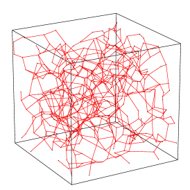
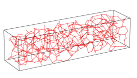
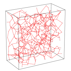
Fig. 11: Illustration of some of the possibilities for modeling rock fracture networks in 3-dimensional space.

To give a flavor of the differences between the 2- and 3-dimensional RRNGs we study here the change in the average degree, the diameter, the algebraic connectivity and the diffusion time with the elongation in the 2- and 3-dimensional RRNGs. To make things comparable we study here only the case one side of the cube changes, say $1\leq a\leq 5$ in steps for $0.5$, keeping b=1/a and $c=1$. As for the case of the 2D graphs, the elongation of the cube produces a decay of the average degree, an increase of the diameter and a decrease of the algebraic connectivity. The resulting effects on the diffusion is that elongation delays the diffusion process. It happens, as expected, that the average degree of the 3D RRNG is larger than that of the 2D analogue. This is due to the fact that nodes can now be connected in three directions of space instead of two. More interestingly, the increase of the diameter of the 3D model is much slower than that in the case of the 2D one. For instance, the diameter increases almost linearly with the elongation according to $D\approx 14.8+40.66a$ for the 2D case, while it is $D\approx 11.1+13.53a$ for the 3D case. That is, the growth of the diameter in the 3D model studied is almost four times slower than in the 2D case for similar elongations. These results can be understood by adapting our previous bound for the 3D case. In this case we should consider that the separation between the points in the 3D cube is given by $1/\sqrt[3]{n}$, such as

$$D\left(G\right)\geq\sqrt[3]{n}\dfrac{\sqrt{\left(a^{4}+1\right)}}{a}.$$ (30)

Then, it is clear that the diameter of the 3D RRNGs grows more slowly than that of the 2D ones. This of course produces a dramatic decay of the algebraic connectivity with the elongation in the 3D model ($\mu_{2}=0.0246a^{-1.87}$), where this parameter drops much faster with the elongation than in the 2D case ($\mu_{2}=0.00307a^{-1.92}$). The main consequence of this elongation effect is observed in the slower growth of the diffusion time for the cuboid model than for the rectangular one. While in the 2D case the diffusion time increases as $\left\langle t_{c}\right\rangle\approx 0.064+0.093a$ with the elongation, in the 3D case it grows as $\left\langle t_{c}\right\rangle\approx 0.059+0.028a$. That is, the elongation of the cuboid seems to have an effect on the diffusion time which is three times smaller than the effect of elongation of the rectangle.

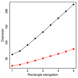
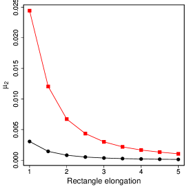
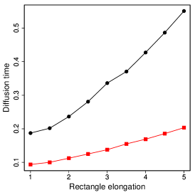
Fig. 12: Comparison of the effects of elongation on the diameter, algebraic connectivity and diffusion time in 2- (black dots) and 3-dimensional (red squares) RRNGs having $n=1000$ nodes.

In closing we can think that the combination of the three effects studied here as potential extensions of our model will make the diffusion of oil and gas much faster than what we have predicted using the normal 2D diffusion model with constant apertures of the fractures. That is, if we consider apertures larger than one, include long-range hops of the diffusive particles and consider a 3D space instead of a 2D one, we will observe super-fast diffusion on the rock fracture networks studied. We should consider such combinations when some experimental data is available, which permit us to compare our theoretical predictions with reality.

9 Conclusions

We have developed a model based on a generalization of the random neighborhood graphs which reproduces very well the structural and dynamical properties of real-world rock fracture networks. The properties of small rock fracture networks are well-described by using the newly developed random rectangular neighborhood graph for small values of the rectangular elongation. In contrast, larger RFNs are better described by RRNGs with significantly longer elongations. This means that small RFNs are embedded into more spherical rocks than the larger ones, which are mainly embedded into rocks with a higher aspect ratio. The most important characteristic of the RRNG is that it makes it possible to study a large variety of structural and dynamical processes by changing some of the parameters of the model. In such a way we can be more independent of the existence of appropriate datasets of real-world RFNs, which in many cases are scarce.

As has been seen in this work, the heat equation adapted to consider the graph as the space in which the diffusive process is taking place is an appropriate tool for studying the diffusion of oil and gas on RFNs. This work also studies the relationship between the structure of rock networks and the diffusion dynamics taking place on them. In particular, a set of a few structural parameters were obtained that describe well the diffusive process taking place on the networks. Of special interest is the second smallest eigenvalue of the Laplacian matrix, which shows a correlation coefficient larger than $0.99$ with the average diffusion time on RFNs. This index is then a very good predictor of the capacity of a given network to diffuse substances through the channels produced by the fractures in the rock.

Finally we have considered a few potential extensions of our model. They include the consideration of variable fracture apertures, the possibility of long-range hops of the diffusive particles as a way to account for heterogeneities in the medium and possible superdiffusive processes, and the extension of the model to consider 3-dimensional modeling scenarios. These potential additions show the generality and flexibility of our model to accommodate new structural and dynamical characteristics to better reflect the physical reality to be modeled.

All in all, we consider that the newly proposed model based on random rectangular neighborhood graphs is very flexible and can be adapted to specific simulation requirements and is therefore appropriate to model RFNs in a variety of scenarios.

10 Acknowledgment

The authors thank E. Santiago et al. for providing the datasets of rock fracture networks used in this work. Any request of this dataset should be addressed to: esantiago@im.unam.mx. M. S. thanks financial support from the Weir Advanced Research Centre at the University of Strathclyde. E. E. thanks the Royal Society for a Wolfson Research Merit Award. EE also thanks Jorge X.Velasco-Hernández for introducing him to this fascinating world of rock fracture networks.

Appendices

Appendix A

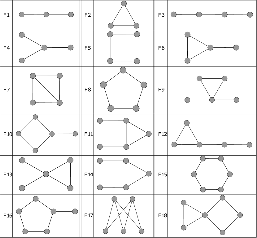
Fig. 13: Illustration of the structure of the small subgraphs used as structural descriptors in this work.

Appendix B

⬇

-diag(diag(A));

n=length(A);

u=ones(n,1);

t=diag(A^3);

k=A*u;

k1=k-1;

k2=k-2;

m=sum(k)/2;

%Auxiliary functions

Q=A^2.*A;

P=0.5*A^2.*(A^2-1);

q=diag(A^5);

b=0.5*(q-5*t-2*(t.*k2)-2*Q*k2-2*(0.5*A*t-Q*u));

R=(1/6)*(A^2.*(A^2-1).*(A^2-2));

%Fragments according to book

F1=0.5*(k'*k1);

F2=(1/6)*sum(t);

F3=0.5*(k1'*A*k1)-3*F2;

F4=(1/6)*(k.*k1)'*k2;

F5=(1/8)*(trace(A^4)-4*F1-2*m);

F6=0.5*(t'*k2);

F7=0.25*u'*(Q.*(Q-A))*u;

F8=(1/10)*(trace(A^5)-10*F6-30*F2);

F9=0.25*(k2.*(k2-1))'*t;

F10=u'*(P-diag(diag(P)))*k2-2*F7;

F11=0.5*(k2'*Q*k2)-2*F7;

F12=0.5*u'*(A^2-diag(diag(A^2)))*t-6*F2-2*F6-4*F7;

F13=0.25*t'*(0.5*t-1)-2*F7;

F14=0.5*u'*(Q.*(A^3.*A))*u-9*F2-2*F6-4*F7;

F15=(1/12)*(trace(A^6)-2*m-12*F1-24*F2-6*F3-12*F4-48*F5-36*F7-12*F10-24*F13);

F16=k2'*b-2*F14;

F17=0.5*(u'*(R.*A)*u);

F18=0.5*(u'*(P-diag(diag(P)))*t)-6*F7-2*F14-6*F17;

%Results in the form of a column vector

S=[F1 F2 F3 F4 F5 F5 F7 F8 F9 F10 F11 F12 F13 F14 F15 F16 F17 F18]';

Algorithm 1 Matlab code used for the calculation of the 18 small subgraphs illustrated in Fig. (13).

Appendix C

⬇

ction [graph,p] = beta(n,beta,lengths,p)

%Output 'graph' as adjacency list and list of coordinates 'p'

%can use cell2mat on output graph to get adjacency matrix

%

%beta=0 is the complete graph %beta=1 is the Gabriel graph

%beta=2 is the RNG

%

%If no lengths given, a unit square is assumed.

%If one length given, unit area is assumed.

%

%functions being called use beta differently, so the value is converted via

%beta_other=(1-beta)/(1+beta): [0,inf]->[1,-1]

%

%You can also supply the coordinates 'p' yourself as an n*2 matrix

if ~exist('beta','var')

error('Please supply a value for beta')

end

if ~exist('n','var')

error('Please supply the number of nodes')

end

if beta<0

error('Beta must be non-negative')

end

if ~exist('lengths','var')

lengths=[1 1];

elseif length(lengths)==1

lengths=[lengths 1/lengths];

end

if ~exist('p','var')

p=[unifrnd(0,lengths(1),n,1) unifrnd(0,lengths(2),n,1)];

end

if beta==0

graph=CompleteGraph(n);

elseif beta==1

dataDist=distFast(p,p);

[~,indall]=sort(dataDist,'ascend');

graph=GabrielGraph(p,indall);

elseif beta==2

dataDist=distFast(p,p);

graph=RelativeNeighborhoodGraph(dataDist);

else

beta=(1-beta)/(1+beta);

dataDist=distFast(p,p);

graph=LuneBetaSkeletonGraph(p,dataDist,beta);

end

end

Algorithm 2 Matlab code used for creating rectangular $\beta$-skeleton graphs, which makes use of an available toolbox (Aupetit (2016)).

References

- Adler and Thovert (1999) P.M. Adler, J.F. Thovert, Fractures and Fracture Networks. Theory and Applications of Transport in Porous Media (Springer, Netherlands, 1999). ISBN 9780792356479
- Albinali et al. (2016) A. Albinali, R. Holy, H. Sarak, E. Ozkan, Modeling of 1d anomalous diffusion in fractured nanoporous media. Oil Gas Sci. Technol. - Rev. IFP Energies nouvelles 71(4), 56 (2016). doi:10.2516/ogst/2016008
- Andersson and Dverstorp (1987) J. Andersson, B. Dverstorp, Conditional simulations of fluid flow in three-dimensional networks of discrete fractures. Water Resources Research 23(10), 1876–1886 (1987). doi:10.1029/WR023i010p01876
- Andresen et al. (2012) C.A. Andresen, A. Hansen, R. Le Goc, P. Davy, S. Mongstad Hope, Topology of fracture networks. ArXiv e-prints (2012). doi:10.3389/fphy.2013.00007
- Aupetit (2016) M. Aupetit, Matlab: Proximity graphs toolbox, 2016. http://www.mathworks.com/matlabcentral/fileexchange/55303-proximity-graphs-toolbox
- Barton (1995) C.C. Barton, Fractal Analysis of Scaling and Spatial Clustering of Fractures, ed. by C.C. Barton, P.R. La Pointe (Springer, Boston, MA, 1995), pp. 141–178. 978-1-4899-1397-5
- Berkowitz (2002) B. Berkowitz, Characterizing flow and transport in fractured geological media: A review. Advances in Water Resources 25(8-12), 861–884 (2002). doi:10.1016/S0309-1708(02)00042-8
- Bogatkov and Babadagli (2007) D. Bogatkov, T. Babadagli, Characterization of fracture network system of the midale field, in Canadian International Petroleum Conference, Petroleum Society of Canada, 2007. Petroleum Society of Canada. doi:10.2118/2007-031
- Bonnet et al. (2001) E. Bonnet, O. Bour, N.E. Odling, P. Davy, I. Main, P. Cowie, B. Berkowitz, Scaling of fracture systems in geological media. Reviews of Geophysics 39(3), 347–383 (2001). doi:10.1029/1999RG000074
- Cacas et al. (1990) M.C. Cacas, E. Ledoux, G. de Marsily, A. Barbreau, P. Calmels, B. Gaillard, R. Margritta, Modeling fracture flow with a stochastic discrete fracture network: Calibration and validation: 2. the transport model. Water Resources Research 26(3), 491–500 (1990). doi:10.1029/WR026i003p00491
- Camacho Velazquez et al. (2012) R. Camacho Velazquez, M.A. Vasquez-cruz, G. Fuentes-Cruz, Recent advances in dynamic modeling of naturally fractured reservoirs, Offshore Technology Conference, 2012. Offshore Technology Conference. doi:10.4043/23195-MS
- Damjanac and Cundall (2013) B. Damjanac, P.A. Cundall, Validation of lattice approach for rock stability problems, in 47th US Rock Mechanics/Geomechanics Symposium, American Rock Mechanics Association, 2013. American Rock Mechanics Association
- Edery et al. (2016) Y. Edery, S. Geiger, B. Berkowitz, Structural controls on anomalous transport in fractured porous rock. Water Resources Research 52(7), 5634–5643 (2016). doi:10.1002/2016WR018942
- Estrada (2000) E. Estrada, Characterization of 3d molecular structure. Chemical Physics Letters 319(5-6), 713–718 (2000). doi:10.1016/S0009-2614(00)00158-5
- Estrada (2010) E. Estrada, Quantifying network heterogeneity. Phys. Rev. E 82, 066102 (2010). doi:10.1103/PhysRevE.82.066102
- Estrada (2011) E. Estrada, The Structure of Complex Networks: Theory and Applications (Oxford University Press, Oxford, 2011). ISBN 9780191613425
- Estrada (2012a) E. Estrada, The communicability distance in graphs. Linear Algebra and its Applications 436(11), 4317–4328 (2012a)
- Estrada (2012b) E. Estrada, Path laplacian matrices: Introduction and application to the analysis of consensus in networks. Linear Algebra and its Applications 436(9), 3373–3391 (2012b). doi:10.1016/j.laa.2011.11.032
- Estrada and Hatano (2007) E. Estrada, N. Hatano, Statistical-mechanical approach to subgraph centrality in complex networks. Chemical Physics Letters 439(1-3), 247–251 (2007). doi:10.1016/j.cplett.2007.03.098
- Estrada and Hatano (2014) E. Estrada, N. Hatano, Communicability angle and the spatial efficiency of networks. ArXiv e-prints (2014)
- Estrada and Rodríguez-Velázquez (2005) E. Estrada, J.A. Rodríguez-Velázquez, Spectral measures of bipartivity in complex networks. Phys. Rev. E 72, 046105 (2005). doi:10.1103/PhysRevE.72.046105
- Estrada et al. (2016) E. Estrada, E. Hameed, N. Hatano, M. Langer, Path laplacian operators and superdiffusive processes on infinite graphs. arXiv preprint arXiv:1604.00555 (2016)
- Fiedler (1973) M. Fiedler, Algebraic connectivity of graphs. Czechoslovak mathematical journal 23(2), 298–305 (1973)
- Garipov et al. (2016) T.T. Garipov, M. Karimi-Fard, H.A. Tchelepi, Discrete fracture model for coupled flow and geomechanics. Computational Geosciences 20(1), 149–160 (2016). doi:10.1007/s10596-015-9554-z
- Han et al. (2013) J.J. Han, T.H. Lee, W.M. Sung, Analysis of oil production behavior for the fractured basement reservoir using hybrid discrete fractured network approach. Advances in Petroleum Exploration and Development 5(1), 63–70 (2013). doi:10.3968/j.aped.1925543820130501.1068
- Hansford and Fisher (2009) J. Hansford, Q. Fisher, The influence of fracture closure from petroleum production from naturally fractured reservoirs: A simulation modelling approach. The Oral Presentation at AAPG Annual Convention, Denver, Colorado, USA (2009)
- Hasan et al. (2012) A. Hasan, B. Foss, S. Sagatun, Flow control of fluids through porous media. Applied Mathematics and Computation 219(7), 3323–3335 (2012). doi:10.1016/j.amc.2011.07.001
- Hewett (1986) T.A. Hewett, Fractal distributions of reservoir heterogeneity and their influence on fluid transport, in SPE Annual Technical Conference and Exhibition, Society of Petroleum Engineers, 1986. Society of Petroleum Engineers
- Hitchmough et al. (2007) A.M. Hitchmough, M.S. Riley, A.W. Herbert, J.H. Tellam, Estimating the hydraulic properties of the fracture network in a sandstone aquifer. Journal of Contaminant Hydrology 93(1-4), 38–57 (2007). doi:10.1016/j.jconhyd.2007.01.012
- Huseby et al. (1997) O. Huseby, J.F. Thovert, P.M. Adler, Geometry and topology of fracture systems. Journal of Physics A: Mathematical and General 30(5), 1415 (1997). doi:10.1088/0305-4470/30/5/012
- Jafari and Babadagli (2012) A. Jafari, T. Babadagli, Estimation of equivalent fracture network permeability using fractal and statistical network properties. Journal of Petroleum Science and Engineering 92-93, 110–123 (2012). doi:10.1016/j.petrol.2012.06.007
- Jang et al. (2013) Y.H. Jang, T.H. Lee, J.H. Jung, S.I. Kwon, W.M. Sung, The oil production performance analysis using discrete fracture network model with simulated annealing inverse method. Geosciences Journal 17(4), 489–496 (2013). doi:10.1007/s12303-013-0034-y
- Jaromczyk and Toussaint (1992) J.W. Jaromczyk, G.T. Toussaint, Relative neighborhood graphs and their relatives. Proceedings of the IEEE 80(9), 1502–1517 (1992). doi:10.1109/5.163414
- Klein and Randíc (1993) D.J. Klein, M. Randíc, Resistance distance. Journal of Mathematical Chemistry 12(1), 81–95 (1993). doi:10.1007/BF01164627
- Koike et al. (2012) K. Koike, C. Liu, T. Sanga, Incorporation of fracture directions into 3d geostatistical methods for a rock fracture system. Environmental Earth Sciences 66(5), 1403–1414 (2012). doi:10.1007/s12665-011-1350-z
- Kowaluk (2014) M. Kowaluk, Planar -skeletons via point location in monotone subdivisions of subset of lunes. ArXiv e-prints (2014)
- Long and Billaux (1987) J.C.S. Long, D.M. Billaux, From field data to fracture network modeling: An example incorporating spatial structure. Water Resources Research 23(7), 1201–1216 (1987). doi:10.1029/WR023i007p01201
- Mohar (1991) B. Mohar, Eigenvalues, diameter, and mean distance in graphs. Graphs and Combinatorics 7(1), 53–64 (1991). doi:10.1007/BF01789463
- Neuman (1988) S.P. Neuman, Stochastic Continuum Representation of Fractured Rock Permeability as an Alternative to the REV and Fracture Network Concepts, ed. by E. Custodio, A. Gurgui, J.P.L. Ferreira (Springer, Dordrecht, 1988), pp. 331–362. 978-94-009-2889-3
- Newman (2002) M.E.J. Newman, Assortative mixing in networks. Phys. Rev. Lett. 89, 208701 (2002). doi:10.1103/PhysRevLett.89.208701
- Nolte et al. (1989) D.D. Nolte, L.J. Pyrak-Nolte, N.G.W. Cook, The fractal geometry of flow paths in natural fractures in rock and the approach to percolation. pure and applied geophysics 131(1), 111–138 (1989). doi:10.1007/BF00874483
- Polubarinova-Kochina (1962) P.Y. Polubarinova-Kochina, Theory of ground water movement princeton university press. Princeton, NJ (1962). doi:10.1126/science.139.3557.820-a
- Santiago et al. (2014) E. Santiago, J.X. Velasco-Hernández, M. Romero-Salcedo, A methodology for the characterization of flow conductivity through the identification of communities in samples of fractured rocks. Expert Systems with Applications 41(3), 811–820 (2014). Methods and Applications of Artificial and Computational Intelligence. doi:10.1016/j.eswa.2013.08.011
- Santiago et al. (2016) E. Santiago, J.X. Velasco-Hernández, M. Romero-Salcedo, A descriptive study of fracture networks in rocks using complex network metrics. Computers & Geosciences 88, 97–114 (2016). doi:10.1016/j.cageo.2015.12.021
- Santiago et al. (2013) E. Santiago, M. Romero-Salcedo, J.X. Velasco-Hernández, L.G. Velasquillo, J.A. Hernández, An Integrated Strategy for Analyzing Flow Conductivity of Fractures in a Naturally Fractured Reservoir Using a Complex Network Metric, ed. by I. Batyrshin, M.G. Mendoza (Springer, Berlin, Heidelberg, 2013), pp. 350–361. 978-3-642-37798-3
- Sarkar et al. (2002) S. Sarkar, M.N. Toksoz, D.R. Burns, Fluid flow simulation in fractured reservoirs, Technical report, Massachusetts Institute of Technology. Earth Resources Laboratory, 2002
- Seifollahi et al. (2014) S. Seifollahi, P.A. Dowd, C. Xu, A.Y. Fadakar, A spatial clustering approach for stochastic fracture network modelling. Rock Mechanics and Rock Engineering 47(4), 1225–1235 (2014). doi:10.1007/s00603-013-0456-x
- Silva et al. (2007) A.T. Silva, E.K. Lenzi, L.R. Evangelista, M.K. Lenzi, L.R. da Silva, Fractional nonlinear diffusion equation, solutions and anomalous diffusion. Physica A: Statistical Mechanics and its Applications 375(1), 65–71 (2007). doi:10.1016/j.physa.2006.09.001
- Snijders (1981) T.A.B. Snijders, The degree variance: An index of graph heterogeneity. Social Networks 3(3), 163–174 (1981). doi:10.1016/0378-8733(81)90014-9
- Toussaint (1980) G.T. Toussaint, The relative neighbourhood graph of a finite planar set. Pattern Recognition 12(4), 261–268 (1980). doi:10.1016/0031-3203(80)90066-7
- Valentini et al. (2007) L. Valentini, D. Perugini, G. Poli, The “small-world” topology of rock fracture networks. Physica A: Statistical Mechanics and its Applications 377(1), 323–328 (2007). doi:10.1016/j.physa.2006.11.025
- Von Collatz and Sinogowitz (1957) L. Von Collatz, U. Sinogowitz, Spektren endlicher grafen. Abhandlungen aus dem Mathematischen Seminar der Universität Hamburg 21(1), 63–77 (1957). doi:10.1007/BF02941924
- Watts and Strogatz (1998) D.J. Watts, S.H. Strogatz, Collective dynamics of ‘small-world’ networks. nature 393(6684), 440–442 (1998). doi:10.1038/30918
- Wilson et al. (2015) T.H. Wilson, V. Smith, A. Brown, Developing a model discrete fracture network, drilling, and enhanced oil recovery strategy in an unconventional naturally fractured reservoir using integrated field, image log, and three-dimensional seismic data. AAPG Bulletin 99(4), 735–762 (2015). doi:10.1306/10031414015
- Xu and Dowd (2014) C. Xu, P.A. Dowd, Stochastic fracture propagation modelling for enhanced geothermal systems. Mathematical Geosciences 46(6), 665–690 (2014). doi:10.1007/s11004-014-9542-1