The Python user interface of the elsA cfd software:
a coupling framework for external steering layers

Abstract

The Python–elsA user interface of the elsA cfd (Computational Fluid Dynamics) software has been developed to allow users to specify simulations with confidence, through a global context of description objects grouped inside scripts. The software main features are generated documentation, context checking and completion, and helpful error management. Further developments have used this foundation as a coupling framework, allowing (thanks to the descriptive approach) the coupling of external algorithms with the cfd solver in a simple and abstract way, leading to more success in complex simulations. Along with the description of the technical part of the interface, we try to gather the salient points pertaining to the psychological viewpoint of user experience (ux). We point out the differences between user interfaces and pure data management systems such as cgns.

1 Introduction

elsA (http://elsa.onera.fr/) is a large cfd software for research and industry, mainly used in aerospace design, for both internal and external flow. It has been described before (Gazaix et al., 2002; Cambier et al., 2011).

Here we will be interested in the extension of the Python–elsA user interface to additional software, for performing simulations not only at a few discrete specified workflow conditions (e.g. given Mach, Reynolds …) but on a domain of variation, i.e. a Design of Experiment space (doe), with several algorithmic layers added above the cfd solver.

The first step is to automate the spanning of a (given) large number of specified points covering the doe. The second one is to add a stabilization layer for prolongation through unstable doe zones (e.g. when the flow conditions lead to separation). The third one is to use the resulting “stabilized spanning” algorithm as a provider of observable quantities for a sparse polynomial interpolator, driving the simulation and selecting the doe points to compute. If successful, this composite algorithm provides (for the chosen observable) an efficient global representation (response surface) allowing further studies on the doe, at low cost; for example stochastic analysis using the Monte-Carlo method on the response surface would be a fourth step.

The specific point of interest of our approach is that, for this complex composite algorithm, we manage to keep the user interface simple and uniform, using the same concepts as for the base interface. Sections 2-4 explain these concepts; sections 5&6 deal with documentation, error messages, and the gui (Graphical User Interface); finally, sections 7-9 deal with high-level operations and how we use them for doe spanning and analysis.

This paper includes a number of elements from the cfd application domain, and software considerations, along with user interface concepts; these concepts (and most of the software implementation) would be applicable to many different domains. Not included here are considerations for field-like data, for which the cfd General Notation System standard (cgns) is better suited.

2 Interface development orientation

2.1 User interaction model

In the development of the Python–elsA user interface, we strived to reach an equilibrium between power and usability, both on the user side (running simulations) and on the developer side (adding functionality); also, we have tried to avoid a steep user learning curve.

The Python–elsA user interface has been used since June 2000 with no change in its base principles (see section 2.2), and thus maybe it is not too far off its target demography. The basic interface is readily extended with additional classes allowing external algorithmic layers, see 8.1, to complement the cfd solver coded in the elsA kernel.

The Python–elsA interface is built on a declarative user interaction model (Wikipedia, 2016a), whereas similar software (Gerhold, 2008) uses an imperative model (Wikipedia, 2016c). The scripts describing the elsA cfd simulations use context sharing to avoid data duplication; and all the tedious details which are possibly automated are kept hidden in the behaviour of the description classes.

The Python language has been a great help in building successive abstract layers. We generally try to go with the Principle of Least Astonishment (Seebach, 2001; Ronacher, 2011), and to facilitate an object-oriented and functional (Wikipedia, 2016b; Backus, 1978a; Hudak, 1989) programming style, here in user scripts.

The (functional) Reverse Polish Lisp (rpl) language of some Hewlett-Packard handheld calculators, with its three language levels (User rpl, System rpl, compiled code) (Wikipedia, 2016d), has been the inspiration for an intermediate language where, as for System rpl, a faster checks-less interpreted code – usually generated on the fly from the User level – may be directly accessed by experts.

In Python–elsA, user interaction is mainly through argument-less method calls; this is possible because the would-be arguments are already known as attribute values of the method’s owner object; these values may originate:

1. from user specification, using the owner object’s set() method, see 3.4.1;

2. from context rules – set() terminator in context-dependent default rules for the owner object – possibly involving dependencies on objects other than the method’s owner, see 4.2.1;

3. using the set() method in the behaviour logic of other objects, possibly also involving context rules (e.g. in coupled problems), see 9.2.

The user interaction model thus includes an explicit part (method calls in the user script) and an implicit part (context rules and other class-specific object behaviour), providing automatically-defined values. The latter part is essential, allowing for a lighter work burden and thus better efficiency and security in problem solving. The potential danger, regarding user confidence, of automatically-defined attribute values is alleviated by the display (view method, see 3.4.2) and introspection features of the interface (show_origin method, see 4.2.4).

2.2 Base principles, user & developer sides

The base elements and principles used in the development of this interface are:

For the user (U) side:

1. declarative model: the problem definition is made up of definitions of the simulation parameters; building the adequate solver (acting) is left to a factory, lower down in the C++ elsA kernel; this separation of roles shields the interface from modifications in the kernel implementation details;

2. object-oriented model: the simulation parameters (elements of the mathematical model) are here represented as attributes of description classes; the whole simulation script (a descriptions container) is also a class instance; scripts include no data, only description creations and a few operations, like <desc>.set(<attribute>, <value>), <desc>.check() or <desc>.compute();

3. implicit hierarchy: the whole simulation data structure is a shallow (four-level) tree of scripts (possibly nested), descriptions, attributes, and values (see 3.3); this tree is not explicitly referenced in interface use;

4. static checks (attribute name and value type/definition domain) are performed by default on attributes , see 4.1;

5. dynamic (contextual) checks are performed on demand to ensure the coherency of the problem description; a context is an instance of either a description class or a script class, both owning a check() method.

6. context-dependent (contextual) default values allow tailoring the software to different trades, see 4.2.4; the origin rule for default values may be traced back through the show_origin() method;

7. keep the user in charge: no automatic modification of his/her input; conflicts may only be resolved by the user, upon notification by the interface;

8. the interface may be used as a standalone checking tool, with no cfd kernel needed;

9. the user interface scope is limited to scalar data: mesh and field data (e.g. files) is referenced without contents checking.

For the developer (D) side:

1. the api (Application Programming Interface) between the user interface and the elsA kernel is based on three basic types – float (floating-point), int (integer) and string – and a few methods and functions, see 3.4;

2. the evolving part of the interface is mainly described through resource files, see section 4, from which the documentation skeleton (LaTeX commands, see 5.2) is automatically generated in a coherent way;

3. functionality may be added through “products”, see 8.1, the Python code for which is simply dropped in the adequate place, defining additional description classes;

4. obsolete elements of the interface, see 4.1.3, may be re-activated for version comparison.

2.3 Naming things

One important aspect of the interface – for which there are no exact rules and only a few general principles – is the naming of the various interface elements (especially attributes and their values), see 2.3. This aspect is more in the realm of linguistics, and must take into account the culture of the users.

Naming is recognized as a hard problem in software (Deissenboeck and Pizka, 2006), and is all the more important when dealing with user interaction. In programming, users better understand long, self-explanatory, names (Krikhaar et al., 2009), but “The nonsense words did surprisingly well …distinctive names are helpful even when they are not meaningful” (Shneiderman, 1997).

It seems then that there is no symmetry between understanding which concept is behind a name and, inversely, remembering which name corresponds to the sought concept. It is probably better not to use long names which may differ only by one or two characters – better use shorter names where the differences stands out – or to use names with easily confused characters (Kupferschmid, 2009). Also, we have chosen the underscore style, e.g. global_timestep, for the user interface rather than “camel casing”, e.g. GlobalTimestep, although the latter seems more popular with programmers (Binkley et al., 2009).

A balance must somehow be found, for users to be able both to read and write scripts without reaching for the documentation at every step. This part of the interface management is probably the most involved with language considerations, and the most dependent on user cultural background (e.g. when reusing variable names from equations).

3 Python–elsA description language

Python–elsA is built upon the Python language to create a standard of creation and modification of description (attributes container) and script (descriptions container) objects. Only the main elements of the language will be described here, hoping they give a taste of the chosen user interaction model. Both for the text-mode and graphical-mode interfaces, we have tried to respect the design principles of (Shneiderman, 1997), with (Clarke, 1986) also as a (more abstract) background.

From then on, the <> brackets will be used with general meaning of “realization” (instance, value, …) of the enclosed symbol (class, attribute, …).

3.1 Description object creation

Creating an instance of the <desc> description class is performed by:

<name> = <desc>(name=’<name>’)

where <name> (without quotes) is the canonical Python reference to the created object and ’<name>’ a text identifier using the same characters. This identifier is used both for allowing forward references (to not yet created objects) and for out-of-memory references, either between computational nodes without shared memory or in databases (for accessing objects directly, not through property search), see 7.1.

Notice: simple test scripts may forgo the <name>= argument, thanks to an automatic canonical name search feature, but this is very costly for large scripts and is precluded in industrial cases.

3.2 Script object creation

The script class is derived from the Python module class, to which context-oriented behaviour is added.

A <script> (script instance) is automatically created in-memory when loading a script file (containing Python code) from the elsA command-line; this is the most common way a <script> object is created.

Internally, this creation is performed through the Python–elsA load() function, of which the simplest call form is:

<script> = load(<script_file_name>)

More scripts may be loaded from the main (root) script, script objects may thus be nested.

3.3 Global tree structure

Building a problem description in Python–elsA implicitly creates a tree, with the enclosing (top-level) script object as root:

• scripts reference (include) description constructors (and other method, or function, calls), but own no attributes;

• a script may reference (include) other scripts, through load() calls;

• a description may reference other descriptions, through attach() calls, e.g. cfd1.attach(mod1, num1);

• descriptions own (contain) attributes;

• attributes have values;

• values may be <float>, <int>, <string>, or None (meaning “no value”, for all types).

Calls to the check() method of scripts and descriptions (both being contexts, see 3.4.2) will transitively traverse the referenced objects (included scripts, included or attached descriptions).

3.4 Methods and functions

We describe below a few methods of description classes, see 3.4.1, and of contexts, see 3.4.2; additionally, the close() function call will end the processing of a script.

3.4.1 Specific methods of description classes

• <desc>.set(<attr>, <valu>): define valu as the value of the attr attribute of the <desc> description class instance;

• <desc>.get(<attr>): return the value of the attr attribute of the <desc> description class instance;

• <desc>.compute(): start the algorithm managed by the desc description class.

3.4.2 Methods of contexts (descriptions and scripts)

Description classes and script classes are both contexts: they all inherit from the context class, and thus share a number of methods, which are shown here (in the simplest syntax).

• <context>.check(): perform contextual checking (using influence, dependency and contextual default rules) on the <context> instance; this method is the defining feature of a context;

• <context>.view(): display a compact (using macro-attributes) representation of the <context> instance, masking all non-coherent attribute values;

• <context>.copy(name=<name>): return a copy of the <context> instance, with the <name> identifier;

• <context>.dump(): dump a compact representation of the <context> instance to a file; dumped scripts may not include explicit control structures (loops and tests), which should be managed by description classes.

3.5 Abstraction & flexibility: redirections

For better abstraction and flexibility, some functions and methods are redirections to lower levels:

• function to root script method;

• script method to rootboot description method.

as explained below in 3.5.1, 3.5.2. These redirections are most powerful when coupling with external layers, see 8.1.

3.5.1 Functions redirected to root script methods

The compute, extract, check and dump functions are indirections to the same-named methods of the top-level root script object. Moreover, the –check and –dump command-line options (clo) trigger the corresponding function call on an explicit close() call or on natural termination of the root script, while the –strict option triggers a check() call before the compute() call.

3.5.2 Script methods redirected to the boot description

The compute (start solver) and extract (build the specified output representation) methods of the current script object are indirections to the same-named methods of the current boot description object, see 8.2.

4 Static and dynamic behaviour

New description classes do appear from time to time, but the main mechanism for the evolution of the Python–elsA interface is the addition of new attributes to existing classes. This is performed by augmenting two resource files, one for static definitions and the other for dynamic (context-related) ones.

All resource files (data defining the class attributes and various contextual rules) are structured using varying combinations of the dictionary and list Python types; these varying combinations are allowed (without additional coding) because Python is a dynamically typed language.

Rather than using a uniform formal schema, different ad hoc grammars are used here for each kind of definition, abusing the expert (if dated) advice: “As far as we were aware, we simply made up the language as we went along.” - John Backus, Developer of Fortran (1957) and inventor of bnf (1959) (Backus, 1978b).

We thus conveniently “forget” the invention of the more formal Backus Normal (later Naur) Form (bnf), and use a homebrewed grammar; this non-formal character introduces a degree of incompleteness, which has not introduced problems so far for the cfd target application field; a few special cases of rule definitions are treated using lambda expressions (anonymous functions for in-lining rule code), with also some regular expression matching in lieu of plain comparison on <string> values.

Using only the basic dictionary and list Python types for these homebrewed grammar definitions makes the corresponding resource files compact and readable, so that developers may actually augment them; they are also very fast to parse. Again referencing (albeit indirectly) John Backus: “Because the customers of the 704 were primarily scientists and mathematicians, the language would focus on allowing programmers to write their formulas in a reasonably natural notation.” (Aiken, 2007).

4.1 Definitions for static behaviour

The definitions for static behaviour (i.e. excluding contextual checks) are centralized in a global file, as a Python module. They include for each attribute:

• a short descriptive text;

• a type (float, integer or string) for the attribute value;

• one or several checking methods, further restricting the definition domain (e.g. <float> type but further restricted to $\mathbb{R}^{*+}$);

• a list of default value mechanisms, among: static (value), dynamic (reference to rule), None;

• optionally, restrictions to modifications of the attribute value, e.g. interface only (not user).

Example:
’phymod’:["""fluid model""",[’S’,’I’], {’euler’:0,’nslam’:1,’nstur’:2}, [CNTX_DEFV,None]]

These definitions are rendered in plain English (along with the context-related items, see 4.2) by the man() function of the interface, see 5.1. Moreover, a number of entries may be defined for each class, defining additional metadata, see 4.1.3.

Part of the attributes definitions (for example inheritance, see 4.1.3) is only finalized at runtime. It is then used to define class singletons, managing the attribute definitions for all the instances of a given class. This allows caching (across same-class instances) the internal representation of the definitions.

4.1.1 Attribute definition details

Description chain

The description chain for each attribute is used by the man() function, the popups in the PyGelsA gui, see section 6, and for generating the skeleton of the User’s Reference Manual, see section 5.

Type and definition domain method(s)

The basic type (float, integer or string) of the values of each attribute is complemented with a list of allowed of values, a (registered) checking method for the definition domain (e.g. “strictly positive” or more complex), or a combination of both. When the type changes between the interface and the kernel, the list of allowed values is replaced with a conversion dictionary.

Default values

The “default values” item may be an explicit value, a reference to the (possibly converted) kernel default value, a reference to a (possibly non-existent) context-dependent (contextual) default value, or a list of such items (e.g. contextual, then “static” safe value). The single None default value means that the attribute has no default value; if moreover the attribute is defined as always required, context checks will return False unless it has been defined by the user.

4.1.2 Macro-attributes

To give structure to the large number of attributes of some classes, they may be grouped into “macro-attributes”, meaning named lists of attributes. Macro-attributes are list-valued and may be managed through set(), get(), view() and generally all methods of the description classes meant for plain attributes (their “atoms”).

A macro-attribute may have several versions with differing lengths, e.g. conservative is always the name of the list of the attributes for the conservative variables, whatever the current number of equations. Specific versions (as declared in the resource file) are internally named e.g. conservative*05, conservative*06 …but on the user side, for input and output, plain conservative is used. This feature is not guaranteed to always provide as easy a grouping of related attributes, but it is quite useful.

In the gui, see section 6, the widgets for macro-attributes appear as foldable groups of “atom” widgets. Folding is automatic on failed influence/dependency rules (meaningless macro-attribute).

4.1.3 Attributes metadata

Additional attributes metadata are structured in class-wide lists for:

• always-required attributes (whose value must be defined);

• obsolete attribute and values, and possibly their current replacement
  (–allow_obsolete clo);

• attribute and values which may be filtered out (–filter clo);

• not yet documented attributes and values (–unlock clo);

• inheritance (with possible modifications) of attribute definitions from other classes.

4.2 Definitions for dynamic behaviour

The definitions for dynamic behaviour are the most important part of the base interface, allowing for context management and thus more abstract problem specification. Context management allows the software to behave differently, according either to a few trade-specific indications, see 4.2.4, or to the current global solving operator (in case of coupling), see 9.2.

4.2.1 Context management

The definitions for dynamic behaviour (i.e. rules for context management) are centralized in a global resource file, as a Python module; the inference engine (for applying these rules) is defined in a separate module. Dynamic behaviour is represented here by the context-dependent features of the interface: influence and dependency rules, and contextual default rules, completed by the traversal of relations created through attach() calls and possibly by the hierarchical structure of scripts (through inclusion).

Each problem description thus introduces a realization of a dynamic structure, whose nodes are linked by contextual influence and dependence relations; this structure is a Directed Acyclic Graph (dag), and not a true tree, because a node may have more than one parent (several influence rules may lead to the same attribute being required). The “Acyclic” word is important (also valid for a tree, of course), because we need to ensure that no rules in the grammar lead to circular checking. The “dynamic” qualifier comes both from the influence and dependence rules and from the context-dependent default values, leading to (possibly) different graph realizations for different user inputs, contrary to the static layout of a cgns tree.

Default values are sought when a rules terminator (an end rule) specifies that an attribute value must be defined, and no such value exists; contextual default rules, see 4.2.4, depend on the current state of the descriptions context. The <desc>.get_or_deft(<attr>) method call returns the best-effort result for the value of the <desc>.<attr> attribute – using available context state (attribute values) and rules – or None if no default value may be computed.

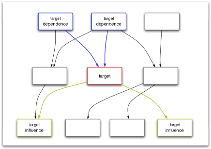
Fig. 1: Contextual dag information flow, through influence and dependency.

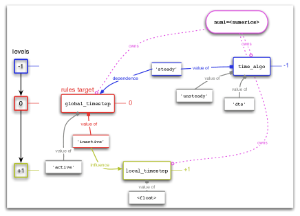
Fig. 2: Local rules evaluation (one attribute).

Each rule is centered on one attribute, Fig. 2, ignoring for the moment the potential complexity which results from traversing all the rules, Fig. 3. When this traversal is performed for a specific case (with user-specified values as initial conditions), a dynamic dag based on contextual relations (context dag) is realized. This dag typically has many levels, quite differently from the flat and static one defined by the class structure, which is used for data storage (and documentation).

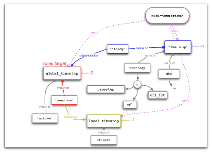
Fig. 3: Global rules traversal (more than one attribute).

Optionally, meaningless values may be “pruned” from the context (using the <desc>.check(prune=True) call), hopefully making it both complete (computable) – using default values – and coherent (here meaning minimal).A simple pruning example would be removing the choice of turbulence model if the simulation is declared laminar, as opposed to a plain <desc>.check() which would only flag the combination as non-coherent.

Pruning may not be fully automated, because the rules system cannot decide on which side of the rule the error lies. Thus, in the spirit below, we will not make a decision to remove the value: "In the face of ambiguity, refuse the temptation to guess." (Peters, 2004).

For example, the user may have kept the turbulent model definition from a previous case, or forgotten to change the flow model from laminar to turbulent when choosing the turbulence model; in this occurrence, a check() call on the involved model object would lead to a Warning-level message, see 5.4.

When performing pruning, the decision is made according to dependency rules, this is why in the above example the turbulent model choice would be removed while the flow model (higher up the context dag) is left unchanged. On the other hand, if unneeded values are defined and the –strict clo is used (or if the corresponding internal option is set from the script), the simulation will be aborted because in this condition all Warnings are bumped to the Error level.

In propagating an initial context of user-defined values using the various contextual rules, we will call “down-propagation” context flow that is centrifugal (propagating away from the root of the context dag), and “up-propagation” context flow that is centripetal, see Fig. 1. A context check may start at any point in the dag, performing both up-propagation (for dependency) and down-propagation (for influence); this is useful for the gui and for interactive user help (what if).

Example rules will be provided for the model class of Python–elsA, which gathers (as attributes) parameters related to the physical model.

4.2.2 Dependency rules

A dependency rule defines the up-propagation of an attribute, and specify that other (source) attributes must have specified values for coherency, see Fig. 1, e.g.:
’visclaw’: {’phymod’: [’nslam’, ’nstur’]}
meaning that the visclaw attribute has meaning only for the ’nslam’ and ’nstur’ (laminar and Navier-Stokes respectively) fluid models, and not for the remaining ’euler’ model, see 4.1.

4.2.3 Influence rules

An influence rule defines the down-propagation of an attribute value, and specify that other (target) attributes must be defined for coherency, see Fig. 1, e.g.:
’visclaw’: {’sutherland’: [’suth_const’, [’suth_muref’, ’suth_muref_fct’], ’suth_tref’]}
meaning that the ’sutherland’ value of the visclaw attribute requires that the suth_const and suth_tref attributes be defined, together with one of suth_muref and suth_muref_fct.

So-called “strong” influence rules specify moreover that the value of the target attribute must belong to a specified list, depending on the value of the origin attribute, e.g.:
’user_config’: {’limited’: [{’turbmod’:[’keps’, ’komega’]}, ’easy’]}
would be a strong rule specifying that when user_config=’limited’ the only possible choices of turbulence model are ’keps’ and ’komega’, and that the ’easy attribute value is required.

4.2.4 Contextual default rules

Contextual default rules provide a mechanism for defining default values of attributes when neither user-defined nor static defaults are provided, e.g.:
’suth_muref’: {1.78938e-5: {’mixture’: [’air’],’cfdpb.units’:[’si’]}}
meaning that the default value of the suth_muref attribute is 1.78938e-5 (in si units), provided that the fluid composition is defined as ’air’ (from the single-element [’air’] list) and the problem is specified in si units.

The dag may be dynamically extended through contextual default rules, which are applied iteratively on a check() call until no new values are defined (or until the maximal iteration count is reached). For each descriptions context state – user-defined values, “static” default values, and current contextual defaults – influence and dependency rules, together with “always required” rules, define which remaining attribute values must be defined to render the context complete. Each newly defined value corresponds to a state transition of this checking automaton.

For all description classes, trade-specific rules (possibly using regular expressions) may be triggered using the user_config attribute with arbitrary <string> values.

All attribute values may be traced to their creator (kernel, user, static default, contextual rule) using the show_origin method. If the creator is a contextual rule, it is listed.

4.2.5 “Horizon” mechanism

An original “horizon” mechanism has been developed (Lazareff, 2009), replacing the definition of various user skill levels with a movable by-attribute boundary across the context-defined dag; it still has to be documented and user-tested.

5 Documentation & error management

5.1 Integrated documentation

The man() function of the interface provides, for any element of the Python–elsA interface (function, class, method, attribute), a compact (and always up-to-date) documentation suitable for a returning user:

man(check)
Name       : check
Type       : function
Description: Check status of root script object

man(view)
Name       : view
Type       : function
Description: Facade for current script’s method

man(model.view)
Name       : view
Type       : instancemethod
Description: Filtering view for a description

man(’phymod’)
1) Attribute name: phymod
2) Class(es)     : model
3) Description   : fluid model
4) Allowed values: ’euler’, ’nslam’, nstur’
5) Rules         :
  5b) influence rules:
    phymod = ’nslam’ requires:
      value(s) for visclaw & prandtl & trans_mod & ...
    phymod = ’euler’ requires:
    phymod = ’nstur’ requires:
      value(s) for visclaw & cv & prandtl &  ...
  5c) context-dependent default values:
    phymod = ’nstur’ IF:
      user_config = ’test::wing’ | ’test::body’ |  ...
  5d) absolute rules:
    attribute value is always required
6) Default value(s): ’euler’
    context-dependent default values in
    ’5c)’, if any, are applied first

Notice: some output lines have been truncated.

When the same attribute name is shared by several classes, the output of man() is factorized across identical definitions.

5.2 User’s Reference Manual updating

A pdf version of the User’s Reference Manual (urm) is built using the LaTeX typographical software (LaTeX project, 2016). For each new version of the elsA software, the urm must be updated with new attribute descriptions (and possibly new functions, classes, methods, and additions to the specialized appendices).

The updating process is partly automated, but requires some human intervention: the CheckDefs tool included in the Python interface code provides automatic generation of the LaTeX source code for the description of the attributes missing in the current urm version, based on the contents of the resource files. Merging in the new LaTeX source is done manually – using the ediff tool in the emacs editor – and coherency of the manual with the interface definitions checked, still using CheckDefs.

5.3 Exceptions (error management)

The Python–elsA interface defines its own exception classes, which use two severity levels:

• WARNING: non-fatal error;

• ERROR: fatal error.

Notice: the –strict clo upgrades all WARNINGs to ERRORs.

5.4 Error messages

The structure of Python–elsA error messages is:

• first line: general information about the error, including the severity level;

• a few lines describing in more detail the problem leading to the error;

• last line: the suggested correction.

It has to be noted that, although these messages on their own appear to be quite explicit, users of our software will sometimes not read the message, instead ringing up elsA software support.

This does not appear to be uncommon (UX User Experience, 2011), and could be linked to user stress, which is what we tried to avoid in the first place, or to a desire not to do a mental “context change” by trying to actually solve the problem themselves: “What they want is to pick up the phone, make a call, and have someone tell them what to do.” (Slashdot, 2010).

6 The PyGelsA gui

The PyGelsA gui (Graphical User Interface) is built on-the-fly using the “static” interface definitions, see 4.1; this means that no modification of the PyGelsA code is needed when updating the user interface for new versions. When loaded with a script, the gui then uses the “dynamic” definitions, see 4.2, for coherency in the display of the description objects.

This display stays coherent thanks to on-the-fly application of context checks. As shown on Fig. 4, attributes with missing required values are labeled in red, while meaningful but user-folded macro-attributes are labeled in green.

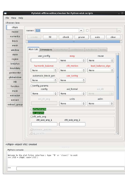
Fig. 4: The PyGelsA gui.

The gui includes (bottom part) a console for text-driven interaction, which is synchronized with the graphical window above. The interface state may later be re-built, either from the logfile or from the file dumped from a dump() call performed at any time during the gui use.

7 Database and network operations

Script (and description) objects may be serialized (transformed into bytecode) and either dumped to/loaded from a database, or accessed through the network.

7.1 Database operations

The script database feature of the interface is built upon a standard underlying database implementation, which may be as simple as a “dictionary on disk”.

A script is an in-memory structure of description objects – and usually some operations– built either from an explicit script file or from code. These operations may be kept “pending” (not executed) if the script is to be stored in a database.

Script databases provide the basic dump/load operations, through the dump() and load() methods. A dumped and re-loaded script will re-create its description objects, and will execute its pending operations, if the environment (mesh files …) is adequate.

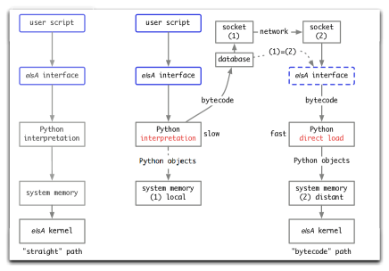
Fig. 5: Database and network use.

These basic operations are complemented by a search() method. For the search to be useful and efficient, the user has to declare a view, defining which parameters (out of possibly several hundred) are of interest for the current study. The <scri>.catalog() method is then called – using this view – at each dump() to update the database’s catalog. The catalog() call may also be used for tagging the output data for the corresponding simulation, providing an authentic traceability (e.g. for plots).

Adequate locking allows the database to be shared in read/write mode between several processes, possibly on different machines, allowing natural parallelism. The default behaviour is to use separate databases for script definition (read-only) and for job execution metadata (read/write) for better efficiency.

The database keeps track of not yet started (NYS), running (RUN), and completed (CMP) state of computational jobs, which helps recovering from crashes, generally using a global <database>.clean() call (resetting all RUN jobs to NYS state) before restart. This partial restarting has been very efficient to reduce user stress, especially when running simulations with more jobs than computing nodes and (clock) execution times counted in days.

7.2 Network operations

Methods for the network class include a simple server/client (sockets) pair, the dump()/load() pair, and the popen() (get command output) and db_search() (find in database) commands.

This functionality allows to access a script database through the network, which is useful when no shared filesystem is available and the underlying database is not networked, see Fig. 5.

8 Extensibility

8.1 Products

So-called “products” are additional (Python) software packages which couple with Python–elsA (and possibly with other products) through description classes. A developer may build a new product (based on the provided skeleton) and simply drop it in the Products directory. Communication between elsA and the added software is performed through an instance of this product-based description class, which contributes to the global context and may get to steer the simulation in lieu of the cfd solver, see section 9.

The algorithm associated with the product may be coded in Python (possibly referencing external packages with compiled libraries) and/or use elsA kernel functionality.

8.2 root and boot objects

If a description class declares a compute() method, an instance of this class may grab control of the simulation from the cfd algorithm, using the global context to gather all the required data. This instance is then called the boot object.

Scripts define a compute() method – invoked in the (top-level root) script through the compute() function – which is an indirection to that of the current boot object; a script with a compute() statement will thus execute differently – without explicit tests – depending on the current boot object, or on the explicit <desc>.compute() call, e.g. (see 9.3):

cfd1 = cfdpb(name=’cfd1’)
cfd1.set(’sfd’, ’active’)
...
dmd1 = dmd(name=’dmd1’)
spr1 = sparse_poly(name=’spr1’)
...
# cfd1.compute() # single-point SFD simulation
# dmd1.compute() # single-point SFD/DMD simulation
compute() # SFD/DMD/SPI coupling on DoE, using spr1

where # starts a comment, and compute() is redirected to spr1.compute() because spr1 is the last-created bootable object.

This logic provides for testing a complex coupling script at different levels with minimal modification; it can also be implemented as:

...
slvrs = {0:cfd1, 1:dmd1, 2:spr1}
slvr_lev = 1 # use dmd1
slvrs[slvr_lev].compute()

The coupling level may thus be specified as an integer value, without any test in the user script.

Lastly, the slvrs[slvr_lev].compute() call above may be replaced by set_boot_objt(<desc>); compute(), where the first statement may be seen as passing a token to <desc>, giving it specific rights. This token may be moved during the simulation, i.e. for collaborating coupling algorithms.

8.3 provide() method for blind creation

When several product-like description objects (e.g. prd1, prd2) use a common description object (e.g. slave), it may occur that it is built by one of them, which should be the first appearing in the script. If for example slave is built by prd1.compute(), built first, and then used by prd2, all is well. But if the boot object is switched from prd1 to prd2, slave will not be built and will miss to both prd1 and prd2, as prd1.compute() is not called anymore.

The solution we use, to avoid here an explicit test on the existence (with possible creation) of slave before each reference, is the use of the provide() method, which wraps the conditional creation, and may be “blindly” called to always return the (new or pre-existent) object.

8.4 target_lift class for target lift computations

The “target lift” functionality allows to replace a standard lifting-body computation, at fixed angle-of-attack (aoa), with the computation of the list of aoas corresponding to the given list of lift values (within convergence bounds).

This is performed by replacing the standard compute() call with one directed to a new <target_lift> boot object, as in:

tcl1 = target_lift(name=’tcl1’)
tcl1.attach(lift)
alphas = compute([0.05, .10, .15])

where lift is an <extractor> defining the computation of the body’s lift and alphas is the aoa output for the specified lift coefficients.

This was the first example of an extension to be finally coded as a product.

8.5 variator class for parametric studies

The variator class allows building script variations from a base version and a list of parameter perturbations, dumping them to a database. Later on this database will be spanned, meaning that all the database scripts will be loaded and pending operations, see 7.1, executed. This is performed in sub-directories of a user-chosen base directory, with all file paths automatically shifted as required. Spanning thus provides the database with an iterator.

A step further, this iterator is made into a more general automaton: during spanning, a simulation may be restarted (chained) from a source simulation, chosen using a user-defined non-isotropic doe distance (in parameter space), possibly with additional rules for restricting the source/target pairing. When chaining simulations, the automaton may also add intermediate points (linearization) to the iteration list, to respect a user-specified maximal jump size in parametric space (Lazareff, 2014).

An external algorithm may also add arbitrary points to the list, see 9.3.

8.6 swarm class for operational efficiency

The swarm class provides an abstraction for a group of spanning simulations. For operational efficiency, automated load management on a computational node is provided either as a maximal count of swarm job instances or as a fraction of the node’s power.

The values of the selected observable quantity, for all the simulations in a swarm, are returned as <valu_list> = <swarm>.compute(), as used for the spi algorithm, 9.3.

9 Design of Experiment studies

Studies in Design of Experiment (doe) space involve at least two levels: the basic automaton performing the space spanning, and the mathematical tools, applied both to each doe point and to the global space. These tools may be passive (using specified doe points in a given order), or they may use observable quantities to steer the spanning automaton, possibly creating new doe points on-the-fly.

In 9.2 and 9.3 we will give two examples in the field of differentiable dynamical systems (the geometrical study of complex systems and their stability) (Smale, 1967) applied to cfd, first as a local study and then on a doe. Usually the system is defined by an equation like $\dot{x}=v(x)$. Here however the operator of the system is unknown, and only accessible through cfd observable quantities at computed points of the doe, so that as a first step we have to address the problem of doe discovery, see 9.1, to ensure that the main features of the operator are accounted for.

9.1 doe spanning and discovery

doe discovery is an extended parametric study, see 8.5, where the aim is to describe (find the main features of) the space inside a closed boundary in parametric space, with possible refinement of the initial set of doe points (Lazareff, 2014). Continuation techniques (e.g. stabilization to cross doe areas with separated flow) may be needed, see 9.2. As a first approach, doe refinement may be manual, but in 9.3 we introduce an automatic refinement algorithm through the spi algorithm (Chkifa et al., 2014), which greatly simplifies user interaction.

The observable quantity here may be the aerodynamic lift or drag, the spectral radius of the global (physical + numerical) operator, or any other quantity of interest.

9.2 Coupling with the sfd and dmd algorithms

Coupling between elsA, the sfd and dmd algorithms has been performed to provide stabilized cfd solutions, initially at a single doe point for the flow around a cylinder (Cunha et al., 2015). The sfd algorithm may be either part of the cfd solver or treated as a wrapper in the encapsulated version (Jordi et al., 2014), with an sfd description class. The dmd algorithm is coded in Python, with a dmd description class. Some parameters of the cfd algorithm (numerics class attribute values) are dependent on the sfd and dmd algorithms through contextual rules.

This work has since been extended to a (Mach, Reynolds) doe using the variator class. Success is still dependent on the adequate adjustment of some parameters, at this time taken to be constant across the doe. For the time being, this aspect is fully dependent on user expertise.

9.3 Coupling with the sfd, dmd, and spi algorithms

The most complex application to date of the extensibility of elsA through the Python–elsA interface is the algorithm described above in 9.2, complemented by Sparse Polynomial Interpolation (spi) (Chkifa et al., 2014) for doe discovery (to be published).

Here the spanning automaton is managed by the spi algorithm, starting with nodes only at the doe summits and progressively enriching the representation with inner points according to a Clenshaw-Curtis distribution.

The cfd results for the chosen observable quantity at each refinement level of the spi algorithm are computed as a swarm, see 8.6.

With a reasonable degree of convergence of the spi algorithm, we hope that this algorithm will lead to an adequate automatic discovery of the doe features.

Conclusion

The basic foundation of the Python–elsA interface, which has been used since the creation of the elsA software, has long been used for the target lift extension, see 8.4. Recently more complex extensions have been introduced for doe studies.

This descriptive interface and associated functionality provides a high level of abstraction for coupling mathematical algorithmic layers with the cfd solver, reducing the tedious part of user’s work and augmenting efficiency in research and applications.

This approach, allowing for collaborative computing, seems to be well suited for projects coupling several simulation kernels.

Perspectives

A rule-based implementation of the currently kernel-side factory, see 2.2 would remove the potential fragility of the current one, where tests are sometimes nested for several levels. A rule only has to be written once, while inner tests may have to be repeated for each branch of the upper level(s). This would benefit to user-side checking by ensuring completeness and coherency of the rules with the actual solver implementation.

The more immediate new development will be stochastic analysis, using the Monte-Carlo method on the response surface of 9.3, introducing the first 4th-level layer algorithm above the elsA interface (5th-level above the cfd kernel).

Contents

1. 1 Introduction
2. 2 Interface development orientation
   1. 2.1 User interaction model
   2. 2.2 Base principles, user & developer sides
   3. 2.3 Naming things
3. 3 Python–elsA description language
   1. 3.1 Description object creation
   2. 3.2 Script object creation
   3. 3.3 Global tree structure
   4. 3.4 Methods and functions
   5. 3.5 Abstraction & flexibility: redirections
4. 4 Static and dynamic behaviour
   1. 4.1 Definitions for static behaviour
   2. 4.2 Definitions for dynamic behaviour
5. 5 Documentation & error management
   1. 5.1 Integrated documentation
   2. 5.2 User’s Reference Manual updating
   3. 5.3 Exceptions (error management)
   4. 5.4 Error messages
6. 6 The PyGelsA gui
7. 7 Database and network operations
   1. 7.1 Database operations
   2. 7.2 Network operations
8. 8 Extensibility
   1. 8.1 Products
   2. 8.2 root and boot objects
   3. 8.3 provide() method for blind creation
   4. 8.4 target_lift class for target lift computations
   5. 8.5 variator class for parametric studies
   6. 8.6 swarm class for operational efficiency
9. 9 Design of Experiment studies
   1. 9.1 doe spanning and discovery
   2. 9.2 Coupling with the sfd and dmd algorithms
   3. 9.3 Coupling with the sfd, dmd, and spi algorithms

Bibliography

Bibliography

-
Aiken (2007)
Aiken, A., 2007. A memorial given at the 2007 conference on programming
language design and implementation.
URL http://theory.stanford.edu/~aiken/other/backus.pdf -
Backus (1978a)
Backus, J., August 1978a. Can programming be liberated from the
von Neumann style ? A functional style and its algebra of programs.
Communications of the ACM 21 (8), 613–641.
URL http://worrydream.com/refs/Backus-CanProgrammingBeLiberated.pdf -
Backus (1978b)
Backus, J., August 1978b. The history of Fortran I, II and
III. ACM SIGPLAN Notices 13 (8), 168.
URL http://www.softwarepreservation.org/projects/FORTRAN/paper/p165-backus.pdf - Binkley et al. (2009) Binkley, D., Davis, M., Lawrie, D., Morrell, C., May 2009. To camelcase or under_score. In: Program Comprehension, 2009. ICPC ’09. IEEE 17th International Conference on. pp. 158–167.
- Cambier et al. (2011) Cambier, L., Gazaix, M., Heib, S., Plot, S., Poinot, M., Veuillot, J., Boussuge, J., Montagnac, M., March 2011. An Overview of the Multi-Purpose elsA Flow Solver. AerospaceLab (2), 1–15.
- Chkifa et al. (2014) Chkifa, A., Cohen, A., Schwab, C., Aug. 2014. High-dimensional adaptive sparse polynomial interpolation and applications to parametric PDEs. Found. Comput. Math. 14 (4), 601–633.
-
Clarke (1986)
Clarke, A. A., Jun. 1986. A three-level human-computer interface model. Int. J.
Man-Mach. Stud. 24 (6), 503–517.
URL http://dx.doi.org/10.1016/S0020-7373(86)80006-2 -
Cunha et al. (2015)
Cunha, G., Passaggia, P.-Y., Lazareff, M., 2015. Optimization of the
Selective Frequency Damping parameters using model reduction. Physics
of Fluids 27.
URL http://scitation.aip.org/content/aip/journal/pof2/27/9/10.1063/1.4930925 -
Deissenboeck and Pizka (2006)
Deissenboeck, F., Pizka, M., Sep. 2006. Concise and consistent naming. Software
Quality Journal 14 (3), 261–282.
URL http://dx.doi.org/10.1007/s11219-006-9219-1 - Gazaix et al. (2002) Gazaix, M., Jollès, A., Lazareff, M., September 8-13 2002. The elsA object-oriented computational tool for industrial applications. Proc. 23rd Congress of International Council of the Aeronautical Sciences, Toronto, Canada.
-
Gerhold (2008)
Gerhold, T., 2008. Tau-overview.
URL http://tau.dlr.de/fileadmin/documents/meetings/2008/pdf/1st-day-theory/Tau-Overview.pdf -
Hudak (1989)
Hudak, P., August 1989. Conception, evolution and application of functional
programming languages. ACM Computing Surveys 21 (3), 359–411.
URL http://haskell.cs.yale.edu/wp-content/uploads/2011/01/cs.pdf - Jordi et al. (2014) Jordi, B. E., Cotter, C. J., Sherwin, S. J., 2014. Encapsulated formulation of the Selective Frequency Damping method. Phys. of Fluids 26, 034101.
-
Krikhaar et al. (2009)
Krikhaar, R., Lämmel, R., Binkley, D., Lawrie, D., Maex, S., Morrell, C.,
2009. Identifier length and limited programmer memory. Science of Computer
Programming 74 (7), 430 – 445.
URL http://www.sciencedirect.com/science/article/pii/S0167642309000343 - Kupferschmid (2009) Kupferschmid, M., 2009. Classical Fortran: Programming for Engineering and Scientific Applications, Second Edition, 2nd Edition. CRC Press, Inc., Boca Raton, FL, USA.
-
LaTeX project (2016)
LaTeX project, 2016. LaTeX – a document preparation system.
URL https://www.latex-project.org/ - Lazareff (2009) Lazareff, M., 2009. Industrialisation du logiciel elsA pour valorisation en partenariat avec des PME/PMI. RT 2/13349 DSNA, Onera.
-
Lazareff (2014)
Lazareff, M., 2014. Towards autonomous discovery of stiff structures in CFD
Design of Experiment space, from random-walk automaton steered by the
"spiral" criterion. Computers and Fluids 99, 67–82.
URL http://www.sciencedirect.com/science/article/pii/S0045793014001467 -
Peters (2004)
Peters, T., August 2004. The Zen of Python.
URL http://www.python.org/dev/peps/pep-0020/ -
Ronacher (2011)
Ronacher, A., September 2011. Python and the principle of least astonishment.
URL http://lucumr.pocoo.org/2011/7/9/python-and-pola/ -
Seebach (2001)
Seebach, P., August 2001. The cranky user: The principle of least astonishment.
URL http://www.ibm.com/developerworks/library/us-cranky10/ - Shneiderman (1997) Shneiderman, B., 1997. Designing the User Interface: Strategies for Effective Human-Computer Interaction, 3rd Edition. Addison-Wesley Longman Publishing Co., Inc., Boston, MA, USA.
-
Slashdot (2010)
Slashdot, 2010. Save your sanity, give up now.
URL https://ask.slashdot.org/story/10/03/01/132219/How-Do-You-Get-Users-To-Read-Error-Messages -
Smale (1967)
Smale, S., 11 1967. Differentiable dynamical systems. Bull. Amer. Math. Soc.
73 (6), 747–817.
URL http://projecteuclid.org/euclid.bams/1183529092 -
UX User Experience (2011)
UX User Experience, 2011. How do I get users to read error messages ?
URL http://ux.stackexchange.com/questions/393/how-do-i-get-users-to-read-error-messages/ -
Wikipedia (2016a)
Wikipedia, 2016a. Declarative programming.
URL https://en.wikipedia.org/wiki/Declarative_programming -
Wikipedia (2016b)
Wikipedia, 2016b. Functional programming.
URL https://en.wikipedia.org/wiki/Functional_programming -
Wikipedia (2016c)
Wikipedia, 2016c. Imperative programming.
URL https://en.wikipedia.org/wiki/Imperative_programming -
Wikipedia (2016d)
Wikipedia, 2016d. RPL language.
URL https://en.wikipedia.org/wiki/RPL_(programming_language)