Ring correlations in random networks

Abstract

We examine the correlations between rings in random network glasses in two dimensions as a function of their separation. Initially, we use the topological separation (measured by the number of intervening rings), but this leads to pseudo-long-range correlations due to a lack of topological charge neutrality in the shells surrounding a central ring. This effect is associated with the non-circular nature of the shells. It is, therefore, necessary to use the geometrical distance between ring centers. Hence we find a generalization of the Aboav-Weaire law out to larger distances, with the correlations between rings decaying away when two rings are more than about 3 rings apart.

I Introduction

The structure of network glasses is often described by continuous random network (CNR) model. In this model, building units form a random network where short-range order is preserved similar to that in crystals but translational long-range order is absent due mainly to distorted bond angles Rosenhain (1927); Zachariasen (1932); Wright and Thorpe (2013). Such structures have been generally studied by models Gupta and Cooper (1990) and diffraction experiments Warren (1992) which have provided invaluable information on short-range and medium-range order, mostly in the form of pair distribution functions (PDFs) Wright (1994); Elliott (1991); Thorpe and Tichỳ (2012); Treacy et al. (2005).

One challenge in using diffraction data is that this only provides average properties such that the structure cannot be reconstructed uniquely. Meanwhile, Scanning Probe Microscopy (SPM) and Electron Microscopy (EM) techniques have radically shortened the resolution limit and recently true atomic resolution images of silica bilayers and other two-dimensional (2D) amorphous surfaces have become available Lichtenstein et al. (2012); Huang et al. (2012). However, high resolution imaging of bulk amorphous materials remains elusive Bürgler et al. (1999). These new results on 2D glasses have opened up numerous opportunities to study the structure of glasses using actual atomic coordinates. Recent work on 2D glasses includes modeling of silica bilayers Wilson et al. (2013); Wilson (2015), ring distribution Kumar et al. (2014), medium-range order Büchner et al. (2016), suitable boundary conditions to recover missing constraints in the surface Theran et al. (2015) and the refinement of experimental samples Sadjadi et al. (2017). Rigidity theory has also uncovered a connection between 2D glasses and jammed disk packings Thorpe (1983); Ellenbroek et al. (2015).

The remarkable images of vitreous bilayer silica (SiO₂) unveil a ring structure which is the characteristic of covalent glasses. But similar underlying structure also can be found in various amorphous materials such as amorphous graphene Kotakoski et al. (2011); Kumar et al. (2012); Büchner et al. (2014). In fact, these atomic materials are members of a larger class of materials (many with larger length scales) collectively known as cellular networks. Examples are foams and grains Sadoc and Rivier (1999), biological tissues Mombach et al. (1993), metallurgical aggregates, geographical structures, crack networks Korneta et al. (1998), ecological territories, Voronoi tessellations Weaire and Rivier (1984); Stavans (1993) and even the universe at large scale Aragón-Calvo (2014) and fractals Schliecker (2001). Given wide range of length scales, formation mechanisms and physical properties, cellular networks have been subject of many studies Gibson and Ashby (1999); Schliecker (2002). Despite the topological resemblance between 2D amorphous systems and other cellular networks, one should note that these materials are microscopic systems with a very different nature of bonds and forces and hence they can shed light on new properties of cellular networks, in particular those related to geometry.

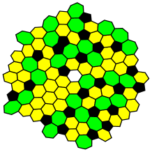
Figure 1: A piece of a two dimensional cellular network generated by bond-switching algorithm from a honeycomb lattice. Rings are colored based on their size. On the bottom left corner, a group of six-fold rings can be seen which also happens in experimental samples and is a feature of amorphous materials, due to statistical correlations. A central six fold ring has been left uncolored and shells of rings will be found around this. Any ring can be used as a central location.

These glassy networks are almost entirely $3-$coordinated networks, i.e., each vertex is connected to three other vertices through edges which form the boundary of polygonal rings (Fig. 1). In the case of amorphous graphene - vertices represent carbon atoms. In silica bilayer, rings are formed by connecting silicon atoms while intervening oxygen atoms are omitted.

These glassy networks, to some extent, are random and their study requires a statistical approach but experimental samples of amorphous materials are relatively small Klemm et al. (2016). Additionally, the small size of many samples does not permit the study of ring correlations at larger distances with good statistics. In this work, we employ large computer models to study correlations among the rings. In the literature, the focus has been on the correlation among adjacent rings where well-known Aboav-Weaire’s law captures the tendency of smaller and larger rings to be adjacent. This paper studies various correlation functions out to large topological and geometrical distances and generalizes the Aboav-Weaire’s law.

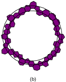
Figure 2: (a): Partitioning of the random network in Fig. 1 into topological shells. The shells grow roughly in circular shapes. This piece also has a triplet inclusion in the forth (blue) shell where a 5-ring is isolated from the fifth (purple) shell. (b) Although shells are roughly circular, no circle can sweep all rings within a single shell; hence ring distributions with topological and geometrical definitions are different.

II Shell analysis and correlations

We define an $n-$ring as a ring with $n$ adjacent rings. The ring distribution of a network with a total of $N$ rings is characterized by $p(n)$, the fraction of $n-$rings, its mean $\left\langle n\right\rangle=\sum_{n}np(n)$, and the second moment about the center $\mu=\left\langle n^{2}\right\rangle-\left\langle n\right\rangle^{2}$. According to Euler’s theorem, mean ring size for a network with periodic boundary conditions (PBCs) is exactly $\left\langle n\right\rangle=6$ . The ensemble average of a quantity $x$ is defined as $\left\langle x\right\rangle=\sum_{n}p(n)x$. To overcome the finite size effect in the experimental samples, we use computer-generated models under PBCs with $\sim$100000 vertices ($\sim$50000 rings) generated from an initially honeycomb lattice using bond-switching algorithm. Here, a bond between two nearest neighbor sites is selected and replaced by a dual bond at right angle and local topology is reconstructed to maintain the three-fold coordination everywhere Wooten et al. (1985); Stone and Wales (1986). Although, experimental samples contain rings with size $4$ to $9$, but fraction of rings with sizes other than $5$ to $7$ are statistically quite rare Kumar et al. (2014). We studied two networks one with only $5$ to $7$ rings and one with $5$ to $8$ but no essential difference was observed. Therefore we report results of the network with $5$ to $8-$fold rings with the following ring distribution: $p(5)=0.262$, $p(6)=0.494$, $p(7)=0.227$, $p(8)=0.0172$ and $\mu=0.558$. Nevertheless, the measures of this paper are general and can be applied to all glassy and cellular networks.

The correlation among rings is usually defined over a topological distance $t$. The topological distance between two rings is defined as the minimum number of bonds should be traversed to connect two rings. This distance is the equivalent of distance of two nodes in the dual graph (when each ring is represented by a node) of Fig. 1. The distance of a ring from itself is zero ($t=0$). All rings which have one common side with a given central ring are located at $t=1$ (first shell). Adjacent rings to the first shell, excluding the central ring, are at $t=2$ (second shell). This process can be continued to find shells at any topological distance similar to Fig. 2. A ring at shell $t$ is adjacent to at least one ring at shell $t-1$ and usually adjacent to at least one ring in shell $t+1$, otherwise this ring is trapped and forms a triplet inclusion (Fig. 2). This definition naturally divides/partitions the network into concentric shells around any given ring. Therefore, all properties of the network are studied as a function of the topological distance and the size of the central ring Fortes and Pina (1993); Mason et al. (2015), as first pointed out by Aste et al Aste et al. (1996a, b).

A shell at distance $t$ from an $n-$ring is characterized by three numbers: number of $n^{\prime}$-rings $N_{t}(n,n^{\prime})$; total number of rings (shell size) $K_{t}(n)$, and total number of sides (edges) $M_{t}(n)$. These quantities are related as follows:

$$K_{t}(n) =\sum_{n^{\prime}}N_{t}(n,n^{\prime}),$$ (1)

$$M_{t}(n) =\sum_{n^{\prime}}n^{\prime}N_{t}(n,n^{\prime}).$$ (2)

Since these equations are linear, they are also valid for the averaged values over all $n-$rings. More importantly, note that $N_{t}(n,n^{\prime})$ is not symmetric in respect to $n$ and $n^{\prime}$. This reflects the fact that local order of the rings is strongly dependent on the size of the central ring. Specially, $N_{t}(n,n^{\prime})$ should not be confused by the number of $n-n^{\prime}$ pairs at topological distance $t$:

$$Np(n)N_{t}(n,n^{\prime})=Np(n^{\prime})N_{t}(n^{\prime},n),$$ (3)

which by definition is symmetric. This symmetry can relate the ensemble average of the number of sides (Eq. 2) to the ensemble average of shell size (Eq. 1) at any topological distance:

$$\left\langle M_{t}\right\rangle =\sum_{n}p(n)M_{t}(n)=\sum_{n}\sum_{n^{\prime}}p(n)n^{\prime}N_{t}(n,n^{\prime})$$

$$=\sum_{n^{\prime}}n^{\prime}p(n^{\prime})K_{t}(n^{\prime})=\left\langle nK_{t}\right\rangle.$$ (4)

This relation is the generalized Weaire sum rule which was originally proposed for the first shell where it takes the form $\left\langle M_{1}\right\rangle=\left\langle n^{2}\right\rangle=\left\langle n\right\rangle^{2}+\mu$ Weaire (1974); Lambert and Weaire (1983). Note that the first shell is the only shell that $K$ is exactly determined $[\,K_{1}(n)=n]\,$ but Eq. II surprisingly encapsulates all the statistical variation in the local ring distribution in a simple form.

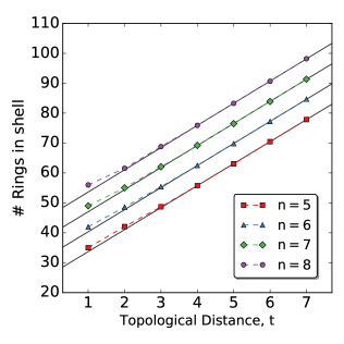
Figure 3: Dependence of the number of rings $K_{t}(n)$ on topological distance $t$ and size of the central ring $n$. $K_{t}(n)$ grows linearly for $t\geq 4$. Solid lines are fitted lines to the last three points. Points are offset for clarity with $6n$.

The space-filling nature of rings in the network requires that $K_{t}(n)$ scales linearly with $t$ in the absence of correlation. This means that the growth rate of the shell size is a constant number independent of the size of the central ring. Although, geometrical constraints on the polygonal tiling of the plane does not allow a complete independence from the central ring simply because shell closure around a larger ring requires more rings. As a result, the intercept of $K_{t}(n)$ remains a function of $n$. Therefore we expect that:

$$K_{t}(n)=At+B(n),$$ (5)

for $t\geq\xi$, where $\xi$ is the ring correlation length. In a hexagonal lattice, the growth rate $A$ is 6 but as Fig. 2 shows, in a random network, shells grow roughly in circular form and simple geometrical arguments predict that the growth rate should be $2\pi$. However, because rings meet each other at random orientations and the shell surface is rough, the actual growth rate is usually greater than $2\pi$ and $A$ can be a measure of this roughness Oguey and Rivier (2001). Figure 3 shows the number of the rings in the shells around different central rings. The linear behavior of the shell size is observed in various systems and is present in 2D glass, as expected. However, in 2D glasses $A=7.31\pm 0.1$ which is much smaller compared to the reported values for Voronoi tessellation ($11.0\pm 0.2$) and soap ($9.45\pm 0.1$) Aste et al. (1996a), probably due to the bond bending interactions which result in the high symmetry (close to the maximum area forgiven edge lengths) of the rings in the 2D glass Kumar et al. (2014).

Another useful quantity is the topological charge of an $n$-ring defined as $6-n$. Since the mean ring size in the network is $6$, equivalently total charge of the network is zero. However a piece of the network can contain any amount of charge depending on the local ring distribution. Hence, topological charge is a useful quantity that monitors the local deviation from the bulk properties. In particular, the topological charge of a shell $q_{t}(n)$ can be defined as the sum of the charge of its rings:

$$q_{t}(n)=\sum_{n^{\prime}}(\left\langle n\right\rangle-n^{\prime})N_{t}(n,n^{\prime})=\left\langle n\right\rangle K_{t}(n)-M_{t}(n).$$ (6)

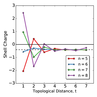
Figure 4: Shell charge $q_{t}(n)$ vs. topological distance $t$. The shell charge settles to a constant non-zero number for $t~{}\geq~{}4$. The dashed line shows the asymptotic offset $-0.4$.

From short- and medium-range order, it is expected that rings around a given ring are distributed such that the charge of the central ring is screened by the charge of the neighboring shells and for $t>\xi$, the ring distribution is similar to the bulk (charge per shell is zero). But as Eq. 5 shows, the shell size is a function of $n$ for any distance and therefore rings are counted with different weights in calculating the charge per shell. In fact, Eqs. II, 5 and 6 readily yield an asymptotic value for the shell charge for $t>\xi$:

$$\left\langle q_{t}\right\rangle=\left\langle(\left\langle n\right\rangle-n)K_{t}\right\rangle\approx p(5)B(5)-p(7)B(7),$$ (7)

which is exact for a network with $n=5,6,7$ and approximately correct as long as fraction of the other rings is negligible. Therefore $\left\langle nK_{t}\right\rangle$ does not factorize and statistically, there is a tendency to have larger rings in a shell $[\,\left\langle q_{t}\right\rangle<0$ since $B(7)>B(5)]\,$ .

The results of calculating the charge per shell is shown in Fig. 4. For $t=1$, the total shell charge has an opposite sign to the charge of the central ring to screen the charge but for $t>1$ screening does not happen and the charge per shell reaches a non-zero constant value, conjectured in Eq. 7. It is interesting to note that although the charge of $5$- and $7$-rings have the same magnitude, the strength of screening for these two is considerably different in the first shell. This shows that geometry has a strong effect on the ring distribution. Note that hexagons have short-range correlations ($\xi=1$) but other rings are correlated up to $\xi=3$ (medium-range correlation) with different strengths.

Topological charge gives a rather complete picture of correlations in the shell structure, but the most studied measure of correlations in the literature is the mean ring size in the first shell around a central ring, through the well-known Aboav-Weaire law that a ring with large size tends to have smaller rings in its neighborhood and vice versa Chiu (1995); Mason et al. (2012). Mathematically, the mean ring size $m_{1}(n)$ around a ring with $n$ neighbors can be written (to a very good approximation) as Aboav (1970); Weaire (1974):

$$nm_{1}(n)=\left\langle n\right\rangle^{2}+\mu+\left\langle n\right\rangle(1-\alpha)(n-\left\langle n\right\rangle),$$ (8)

where $\alpha$ is a fitting parameter which depends on the specific network. Usually a network is characterized by $(\mu,\alpha)$. The meaning of $\alpha$ is not clear but it has been argued that it is a metrical quantity Aboav (1984) or the average excess curvature Mason et al. (2012) but these definitions only work in special cases. In our network, $\alpha\approx 0.23$ which is somewhat smaller than values extracted from experiments Kumar et al. (2014) showing computer generated models still need further refinement.

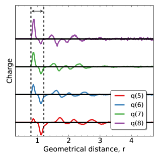
Figure 5: The topological charge $q_{r}(n)$ per shell is plotted against the geometrical distance $r$. The shell charge approaches zero for distances about three rings away. This figure should be compared to Fig. 4. The two dashed lines represent the geometrical distance corresponding to the minimum and maximum values for the first shell with $t=1$. Curves are offset for clarity where horizontal solid lines show the expected asymptotic values of zero.

We would like to extend Aboav-Weaire law to longer distances to study correlation of a ring with the shells around it. The above form can be used to propose a generalized Aboav-Weaire law as:

$$nm_{t}(n)=\left\langle n\right\rangle^{2}+\mu_{t}+\left\langle n\right\rangle(1-\alpha_{t})(n-\left\langle n\right\rangle),$$ (9)

where for $t=1$ we recover Eq. 8 with $\mu_{1}=\mu$. A similar argument presented to derive Eq. 7 can be used to find an asymptotic value for $m_{t}(n)$. At sufficiently long distances, the ring distribution in the shells is independent of the size of the central ring and $\left\langle M_{t}\right\rangle\approx\left\langle m_{t}K_{t}\right\rangle=\left\langle m_{t}\right\rangle\left\langle K_{t}\right\rangle$, therefore for $t>\xi$:

$$\left\langle m_{t}\right\rangle=\frac{\left\langle M_{t}\right\rangle}{\left\langle K_{t}\right\rangle}=\frac{\left\langle nK_{t}\right\rangle}{\left\langle K_{t}\right\rangle}=6-\frac{\left\langle q_{\infty}\right\rangle}{\left\langle K_{t}\right\rangle}.$$ (10)

While we expect $\alpha_{\infty}=0$ but we showed, $\left\langle q_{\infty}\right\rangle<0$, so the asymptotic value of $m_{\infty}(n)$ is larger than the bulk value $6$. For this reason, $m_{t}(n)$ approaches 6 as $t^{-1}$ (since $K_{t}(n)\sim t$) which is sometimes interpreted as a long-range correlation Wang and Liu (2012); Wang et al. (2014). However this should be regarded as an artifact because the shells are defined in such a way (topologically) which results(unfortunately) in the topological charge never going to zero, even at very large distances, and in fact approaching a constant as shown here. This is due to the non-circular nature of the shells, and can be avoided if the shells are chosen in such a way as to make them more nearly circular. Unfortunately this is not possible with a purely topological definition, and so we are forced to adopt a geometrical definition for the ring-shell correlations.

Figure 2 shows the difference between topological and geometrical distance. Despite the fact that shells found by topological distance are roughly circular, it is not possible to find a single circle which contains all the rings in the shell, therefore ring distributions etc. are different in the two cases.

The geometrical distance $r$ between two rings is defined as the Euclidean distance between their centroids. Therefore, instead of using the discrete integer distance $t$, the quantities $q$ and $m$ are written as a function of a continuous distance $r$:

$$q_{r}(n) =6K_{r}(n)-M_{r}(n),$$ (11)

$$nm_{r}(n) =\left\langle n\right\rangle^{2}+\mu_{r}+\left\langle n\right\rangle(1-\alpha_{r})(n-\left\langle n\right\rangle).$$ (12)

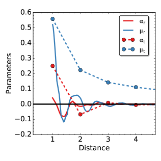
Figure 6: Plot of two coefficients in the generalized Aboav-Weaire law, $\alpha_{r}$ and $\mu_{r}$ with their topological counterparts, $\alpha_{t}$ and $\mu_{t}$. Geometrical definitions show that correlation quickly decays to zero while pseudo-correlations in the topological case last over a long-range for $\mu_{t}$. The geometrical distances are chosen so the geometrical and topological distances agree for the first shell.

Since $r$ is continuous, a binning procedure is used to compare with the previous results using topological distance. Small bins are used with a windowing procedure where the width of the window mimics unity in topological distance. Results for the charge are shown in Fig. 5. It is evident that correlations last about $3$ shells and are quite short-ranged with the charge going to $0$ over the same range, as expected. Therefore this definition of a shell using geometrical distance is more useful. Because of the different size of the rings, e.g., distance between a $5-6$ pair is greater than a $7-8$ pair so a range of geometrical distances corresponds to a single topological distance. To compare the two distances, we rescale the geometrical distance by the average distance between adjacent rings, which is defined to be unity. Fig. 5 shows this for the first neighbors with two dashed lines. Within this window, all four curves show a common trend: a maximum followed by a minimum. The former corresponds to $5-$rings (positively charge) and the latter to $7-$ and $8-$rings (negatively charged). The point in the middle corresponds to neutral $6-$rings. The horizontal axis is normalized such that these three points line up for all curves. According to Aboav-Weaire law, smaller rings surround a larger ring; the pronounced minimum of $q_{r}(5)$ due to $7-$ and $8-$rings and the pronounced maximum of $q_{r}(7)$ and $q_{r}(8)$ due to $5-$rings admit this law. In the case of $q_{r}(6)$, minimum and maximum have the same amplitude due to uniform distribution of the rings around hexagons hence their weak correlations with other rings.

It is also constructive to look at Aboav-Weaire law using geometrical distance. In this case, we expect that both $\alpha_{r}$ and $\mu_{r}$ decay rapidly to zero in accordance with the absence of correlations for large $r$. This is confirmed in Fig. 6 which clearly for distances larger than $3$, the mean ring size is essentially exactly $6$. This confirms our assertion that ring correlations in glassy networks are either short-range or medium-range and using geometrical distance in the calculations of topological charge and mean ring size resolves the issue of excess topological charge in the shells found by topological distance which is shown by the long-tail of $\mu_{2}$ in Fig. 6.

Fig. 7 shows linearity of the generalized Aboav-Weaire law for the third neighbors. The plot shows that $nm(n)$ is indeed a linear function of $n$ but because of pseudo-correlations, the average ring size using topological distance is slightly larger than expected for geometrical distance, where the mean ring size is 6 for three-fold coordinated networks.

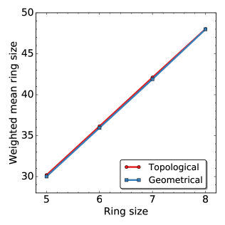
Figure 7: Plot of weighted mean ring size $nm(n)$ versus ring size $n$ for the third neighbors using both geometrical and topological distance. This plot shows that the mean ring size for all shells follows the generalized Aboav-Weaire law (Eq. 9). Note that the topological definition leads to a slightly larger mean ring size.

Although the topological charge and Aboav-Weaire law are useful tools to quantify correlations, they only measure correlations between a ring and shells. The ring-ring correlation function is perhaps a better measure of correlations especially since, as it was shown, definition of shells using the topological distance do introduce some artifacts such as excess charge.

To find out the correlation between two single rings, we need to derive an expression for the probability $p_{t}(n,n^{\prime})$ of finding a pair of $n,n^{\prime}$ rings with distance $t$. For a given $n-$ring, the number of $n^{\prime}-$rings at distance $t$ is $N_{t}(n,n^{\prime})$ while on average a typical shell has $\left\langle K_{t}\right\rangle$ rings. Therefore the probability of having a pair of rings is Szeto et al. (1998):

$$p_{t}(n,n^{\prime})=\frac{p(n)N_{t}(n,n^{\prime})}{\left\langle K_{t}\right\rangle}.$$ (13)

This equation is important as it relates ring distributions of the shell structure to of the network (For $t=1$, this equation reduces to the correlation function defined in Ref. Le Caer and Delannay (1993)). If the rings were independent, this probability is simply product of the individual probabilities but we showed the ring distribution of a shell is different from the bulk and rings are topologically dependent even for large $t$. This motivates us to define the probability of having an $n-$ring at shell $t$ (independent of the central ring) as:

$$p_{t}(n)=\sum_{n^{\prime}}p_{t}(n^{\prime},n)=p(n)\frac{K_{t}(n)}{\left\langle K_{t}\right\rangle},$$ (14)

which can be derived using Eqs. 1 and 3. The probability of having $n-$ring is proportional to the average shell size around $n-$fold rings and the ensemble averaged shell size. We define correlation function between two $n$ and $n^{\prime}$ sided rings as:

$$C_{t}(n,n^{\prime})=p_{t}(n,n^{\prime})-p_{t}(n)p_{t}(n^{\prime})$$ (15)

Figure 8 shows the results for the above correlation function. This clearly shows the medium-range order of the rings except for hexagons where correlations are weak and short-range. In contrast with the results in Ref. Szeto et al. (1998), hexagon-hexagon is short-range and only non-zero for adjacent cells ($t=1$) which is a signature of microcrystal regions in the network (see Fig. 1). If we had used $p(n)p(n^{\prime})$ instead of $p_{t}(n)p_{t}(n^{\prime})$, ring-ring correlation shows a long-range behavior due to topological effect Oguey (2011); Miri and Oguey (2007) but Eq. 14 correctly captures the nature of correlations in the random network.

III Discussion and Conclusion

We have shown that correlations between rings in glassy networks can be treated best if geometrical rather than topological distances between rings are used. Using topological distances, which would be preferable, unfortunately leads to spurious long range correlations as the topological charge for each shell around a central ring does not approach zero at large distances, due to the non-circular nature of the shells. These issues are absent if the geometrical distances between the centers of rings are used. We find in this case that correlations only extend out to about third neighbor rings, and can be described by a generalized Aboav-Weaire law. These studies have been done on a very large computer-generated network with periodic boundary conditions Wooten et al. (1985); Stone and Wales (1986). Experimental samples of bilayer of vitreous silica are currently too small to allow for the study of longer range correlations, but the main conclusion of the paper that geometrical rather than topological distances should be used is expected to hold. Future studies comparing experimental and computer-generated networks (both three-coordinated with similar ring distributions) should help explain why different values of $\alpha$ are obtained in these two cases Kumar et al. (2014).

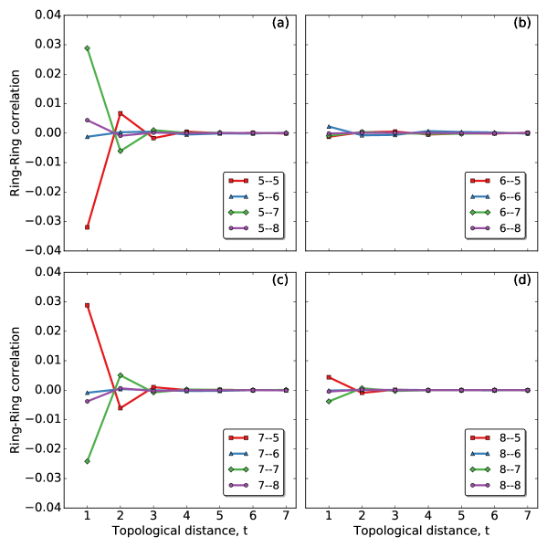
Figure 8: Ring-ring correlation $C_{t}(n,n^{\prime})$ versus topological distance $t$. The correlations are short or medium range depending on the size of the interacting rings. Although hexagons are weakly correlated with their neighbor rings, other rings show a high degree of correlations up to three rings away. Very similar results are obtained using geometrical distances. Note that correlations are symmetric so that $5-6$ is the same as $6-5$ etc. where panel (a) is for five-fold rings, panel (b) six-fold rings, panel (c) seven-fold rings, and panel (d) eight-fold rings.