HyperLogLog Hyper Extended:
Sketches for Concave Sublinear Frequency Statistics

Abstract.

One of the most common statistics computed over data elements is the number of distinct keys. A thread of research pioneered by Flajolet and Martin three decades ago culminated in the design of optimal approximate counting sketches, which have size that is double logarithmic in the number of distinct keys and provide estimates with a small relative error. Moreover, the sketches are composable, and thus suitable for streamed, parallel, or distributed computation.

We consider here all statistics of the frequency distribution of keys, where a contribution of a key to the aggregate is concave and grows (sub)linearly with its frequency. These fundamental aggregations are very common in text, graphs, and logs analysis and include logarithms, low frequency moments, and capping statistics.

We design composable sketches of double-logarithmic size for all concave sublinear statistics. Our design combines theoretical optimality and practical simplicity. In a nutshell, we specify tailored mapping functions of data elements to output elements so that our target statistics on the data elements is approximated by the (max-) distinct statistics of the output elements, which can be approximated using off-the-shelf sketches. Our key insight is relating these target statistics to the complement Laplace transform of the input frequencies.

1. Introduction

We consider data presented as elements $e=(\text{\em{e.key}},\text{\em{e.value}})$ where each element has a key and a positive numeric value $>0$. This data model is very common in streaming or distributed aggregation problems. A well-studied special case is where $\text{\em{e.value}}\equiv 1$ for all elements.

One of the most fundamental statistics over such data is the number of distinct keys: $\operatorname{\textsf{Distinct}}(E)=\{\text{\em{e.key}}\mid e\in E\}$. Exact computation of the statistics requires maintaining a structure of size that is linear in the number of distinct keys. A pioneering design of Flajolet and Martin (FlajoletMartin85, ) showed that an approximate count can be obtained in a streaming model using structures (“sketches”) of logarithmic size. Since then, a rich research strand proposed and analysed a diverse set of approximate counting sketches and deployed them for a wide range of applications (hyperloglogpractice:EDBT2013, ).

Distinct counting sketches can be mostly classified as based on sampling (MinHash sketches) or on random projections (linear sketches). Both types of structures are mergeable/composable: This means that when the elements are partitioned, we can compute a sketch for each part separately and then obtain a corresponding sketch for the union from the sketches of each part. This property is critical for making the sketches suitable for parallel or distributed aggregation.

The original design of (FlajoletMartin85, ) and the leading ones used in practice use sample-based sketches. In particular, the popular Hyperloglog sketch (hyperloglog:2007, ) has double logarithmic size $O(\epsilon^{-2}+\log\log n)$, where $n$ is the number of distinct keys and $\epsilon$ is the target normalized root mean squared error (NRMSE). Since this size is necessary to represent the approximate count, Hyperloglog is asymptotically optimal. We note that the Hyperloglog sketch contains $\epsilon^{-2}$ registers which store exponents of the estimated count. Thus, explicit representation of the sketch has size $O(\epsilon^{-2}\log\log n)$, but one can theoretically use instead a single exponent and $\epsilon^{-2}$ constant-size offsets (e.g. (KNW:PODS2010, ; ECohenADS:TKDE2015, )) to bring the sketch size down to $O(\epsilon^{-2}+\log\log n)$, albeit by somewhat increasing updates complexity. Another point is that Hyperloglog uses random hash functions which have logarithmic-size representations. Some theoretical lower bounds consider the hash representation to be part of the sketch (ams99, ; KNW:PODS2010, )), implying a logarithmic lower bound on size. We follow (FlajoletMartin85, ; hyperloglog:2007, ) and consider the hash representation to be provided by the platform, which is consistent with practice where hash functions are reused and shared by multiple sketches.

We now consider other common statistics over elements. In particular, statistics expressed over a set of (key, weight) pairs, where the weight $w_{x}$ of a key $x$, is defined to be the sum of the values of data elements with key $x$:

$$w_{x}=\sum_{e\mid\text{\em{e.key}}=x}\text{\em{e.value}}\ .$$

Keys that are not active (no elements with this key) are defined to have $w_{x}=0$. Note that if all elements have value equal to $1$, then $w_{x}$ is the number of occurrences of key $x$. For a nonnegative function $f(w)\geq 0$ such that $f(0)\equiv 0$, we define the $f$-statistics of the data as $\sum_{x}f(w_{x})$. We will find it convenient to work with the notation $W(w)$ for the number of keys with $w_{x}=w$. Equivalently, we can treat $W$ as a distribution over weights $w_{x}$ that is scaled by the number of distinct keys. We can then express the $f$-statistics (with a slight notation abuse) as

(1) $$f(W)=\int_{0}^{\infty}W(w)f(w)dw\ .$$

The design og sketches that approximate $f$-statistics over streams of elements was formalized and popularized in a seminal paper by Alon, Matias, and Szegedy (ams99, ). The aim was to understand the necessary sketch size for approximating different statistics and in particular understand which statistics can be sketched in size that is polylogarithmic in the number of keys.

We focus here on functions $f$ that are concave with (sub)linear nonnegative growth-rate. Equivalently, these are all nonnegative linear combinations (the nonnegative span) of capping functions

$$\textsf{cap}_{T}(x)=\min\{T,x\}\ \text{parameterized by}\ T>0\ ,$$

and we therefore use the notation $\overline{\textsf{cap}}$. Members of $\overline{\textsf{cap}}$ that parametrize a spectrum between distinct count ($f(x)=1$) and sum ($f(x)=x$) include frequency moments $f(x)=x^{p}$ in the range $p=[0,1]$ (sum is $p=1$ and distinct count is $p=0$), capping functions (sum is realized by $\textsf{cap}_{\infty}$ and distinct count by $\textsf{cap}_{1}$ when element values are integral and by $f(x)=\textsf{cap}_{T}/T$ as $T\rightarrow 0$ generally), and the soft capping functions

(2) $$\widetilde{\textsf{cap}}_{T}=T(1-\exp(-x/T))\ .$$

Soft capping is a smooth approximation of “hard” capping functions: For $x\ll T$ we have $\widetilde{\textsf{cap}}_{T}(x)\approx x=\textsf{cap}_{T}(x)$, for $x\gg T$ we have $\widetilde{\textsf{cap}}_{T}(x)\approx T=\textsf{cap}_{T}(x)$, and it always holds that

(3) $$\forall x,\,(1-1/e)\textsf{cap}_{T}(x)\leq\widetilde{\textsf{cap}}_{T}(x)\leq\textsf{cap}_{T}(x)\ .$$

Other important $\overline{\textsf{cap}}$ members are $\log(1+x)$ and capped moments.

Statistics in $\overline{\textsf{cap}}$ are used in applications to decrease the impact of very frequent keys and increase the impact of rare keys. It is a common practice to weigh frequencies, say degree of nodes in a graph (NandanwarM:kdd2016, ) or frequency of a term in a document (SaltonBuckley1988, ), by a sublinear function such as $w^{p}$ for $p\in(0,1)$ or $\log(1+w)$. In many applications, the ability to approximate the statistics over the raw data, without the cost of aggregation, can be very useful. One such application is to online advertising (GoogleFreqCap, ; facebookFreqCap, ), data elements are interpreted as opportunities to show ads to users (keys) that are interacting with various apps on different platforms. An advertisement campaign specifies a maximum number of times $T$ an ad can be displayed to the same user, so the number of qualifying impressions corresponds to $\textsf{cap}_{T}$ statistics of the data. Statistics are computed over past data in order to estimate the number of qualifying impressions when designing a campaign. Another application is the computation of word embeddings. The objective is to have the focus and context embeddings of words captures the respective co-occurrence frequencies. Glove (PenningtonSM14:EMNLP2014, ) achieved significant improvements by using $f(w)=\min\{1,w/T\}^{\alpha}$ for $\alpha<1$ (instead of $f(w)=w$). Typically, the text corpus is presented as complete text documents, and elements in arbitrary order are extracted in a pass over this data.

There is a very large body of work on the topic of approximating statistics over streamed or distributed data and it is not possible to mention it all here. Most of the prior work uses linear sketches (random linear projections). A sketch for the second moment, inspired by the JL transform (JLlemma:1984, ), was presented by (ams99, ). Indyk (indyk:stable, ) followed with a beautiful construction based on stable distributions of sketches of size $O(\epsilon^{-2}\log^{2}n)$ for moments in $p\in[0,2]$. Braverman and Ostrovsky (BravermanOstro:STOC2010, ) presented a characterization and an umbrella construction of sketch structures, based on $L_{2}$ heavy hitter sketches, for all monotone $f$-statistics. The structure size is polylogarithmic but is practically too large (degree of the polylog and constant factors).

Sample-based sketches for $\overline{\textsf{cap}}$ functions were presented by the author (freqCap:KDD2015, ). The sketch is a weighted sample of keys that supports approximate cap-statistics on domain queries (subsets of the keys). The framework generalizes both distinct reservoir sampling (Knuth2f, ; Vit85, ) and the sample and hold stream sampling (GM:sigmod98, ; EV:ATAP02, ; flowsketch:JCSS2014, ). The size and quality tradeoffs of the sample are very close (within a small constant) to those of an optimal sample that can be efficiently computed over aggregated data (set of key and weight pairs). Roughly, a sample of $O(\epsilon^{-2})$ keys suffices to approximate $\textsf{cap}_{T}(W)$ unbiasedly with coefficient of variation (CV) $\epsilon$. Moreover, a multi-objective (universal) sample (see (multiw:VLDB2009, ; multiobjective:2015, )) of $O(\epsilon^{-2}\log n)$ keys can approximate with CV $\epsilon$ any $f$-statistics for $f\in\overline{\textsf{cap}}$. When this method is applied to sketching statistics of the full data, we can hash key identifiers to size $O(\log n)$ (to obtain uniqueness with very high probability) and obtain sketches of size $O(\epsilon^{-2}\log n)$ and a multi-objective sketches of size $O(\epsilon^{-2}\log^{2}n)$. One weakness of the design is that these sketches are not fully composable: They apply on streamed elements (single pass) or take two passes over distributed data elements.

A remaining fundamental challenge is to design composable sketches of size $O(\epsilon^{-2}\log n)$ for each $\overline{\textsf{cap}}$ statistics and a composable multi-objective sketch of size $O(\epsilon^{-2}\log^{2}n)$. Given the practical significance of the problem, we seek simple and highly efficient designs. A further theoretical challenge is to design sketches that meet or approach the double-logarithmic representation-size lower bound of $O(\epsilon^{-2}+\log\log n)$.

Contributions overview and organization

We address these challenges and make the following contributions. We show that any statistics in the soft capping span $\overline{\widetilde{\textsf{cap}}}$ can be approximated with the essential effectiveness and estimation quality of Hyperloglog. That is, we present composable sketches of size $O(\epsilon^{-2}+\log\log n)$ that estimate the statistics with RNMSE $\epsilon$ with good concentration. The soft capping span $\overline{\widetilde{\textsf{cap}}}\subset\overline{\textsf{cap}}$ is the set of functions that can be expressed as

(4) $$f(w)=\int_{0}^{\infty}a(t)(1-e^{-wt})dt\ ,\text{ where }a(t)\geq 0\ .$$

In particular, the span includes all soft capping functions, low frequency moments ($f(w)=w^{p}$ with $p\in(0,1)$), and $\log(1+w)$. We also present a composable multi-objective sketch for $\overline{\widetilde{\textsf{cap}}}$. This is a single structure that is larger by a logarithmic factor than a single distinct counter and supports the approximations of all $\overline{\widetilde{\textsf{cap}}}$ statistics. Finally, we consider statistics in $\overline{{\textsf{cap}}}$ that are not in $\overline{\widetilde{\textsf{cap}}}$ and show how to approximate them within small relative errors (12%) using differences of approximate $\overline{\widetilde{\textsf{cap}}}$ statistics.

Our main technical tool is a novel framework, illustrated in Figure 1, that reduces the approximation of the more general statistics to distinct-count statistics. At the core we specify randomized functions $M$ that map data elements of the form $e=(\text{\em{e.key}},\text{\em{e.value}})$ to sets of output elements. Each output element $e^{\prime}\in M(e)$ contains an output key (outkey) $e^{\prime}.key$ (which generally is from a different domain than the input keys) and an optional value $e^{\prime}.value\geq 0$. For a set of data elements $W$, we obtain a corresponding multiset of output elements

$$E=M(W)=\bigcup_{e\in W}M(e)\ .$$

The mapping functions are crafted so that the approximate statistics of the set of data elements $W$ can be obtained from approximations of other statistics of the output elements $E$. In particular, if we have a composable sketch for the output statistics, we obtain a composable sketch for the target statistics. Note that our mapping functions are randomized, therefore the set $E$ is a random variable and so is any (exact) statistics on $E$. We will use approximate statistics on $E$.

The output statistics we use are the distinct count $\operatorname{\textsf{Distinct}}(E)$, which allows us to leverage approximate distinct counters as black boxes, and the more general max-distinct statistics $\operatorname{\textsf{MxDistinct}}(E)$, defined as the sum over distinct keys of the maximum value of an element with the key:

$$\operatorname{\textsf{MxDistinct}}(E)=\sum_{x}m_{x}\ ,$$

$$\text{ where }m_{x}\equiv\max_{e\in E\mid\text{\em{e.key}}=x}\text{\em{e.value}}\ ,$$

which also can be sketched in double logarithmic size. Note that when all elements have value $1$, $\operatorname{\textsf{MxDistinct}}(E)=\operatorname{\textsf{Distinct}}(E)$.

For multi-objective approximations we use all-threshold sketches that allows us to recover, for any threshold $t>0$, an approximation of

(6) $$\operatorname{\text{{\sf TDistinct}}}_{t}(E)=\operatorname{\textsf{Distinct}}\{e\in E\mid\text{\em{e.value}}\leq t\},$$

which is the number of distinct keys that appear in at least one element $e\in E$ with value $\text{\em{e.value}}\leq t$. The size of the all-threshold sketch is larger by only a logarithmic factor than the basic distinct count sketch. We refer to the value of the output statistics on the output elements as a measurement of $W$. When a sketch is applied to approximate the value of output statistics, we refer to the result as an approximate measurement of $W$.

Figure 1. Element processing framework

The paper is organized as follows. In Section 2 we define the complement Laplace transform $\operatorname{\mathcal{L}^{c}}[W](t)$ of the frequency distribution $W$, which is its distinct count minus its Laplace transform at $t$. We have the relation

$$T\operatorname{\mathcal{L}^{c}}[W](1/T)=\widetilde{\textsf{cap}}_{T}(W)\ ,$$

that is, the transform at $1/T$ multiplied by $T$ is the $\widetilde{\textsf{cap}}_{T}$ statistics of the data. In Section 3 we define a mapping function for any $t>0$, so that $\operatorname{\mathcal{L}^{c}}[W](t)$, and hence $\widetilde{\textsf{cap}}_{1/t}$-statistics, is approximated by the respective $\operatorname{\textsf{Distinct}}$ measurement. We refer to this as a measurement of $\operatorname{\mathcal{L}^{c}}[W]$ at point $t$.

In Section 4 we consider the span $\overline{\widetilde{\textsf{cap}}}$ of soft capping statistics, that is, all $f$ of the form (4). Equivalently, $a(t)$ is the inverse $\operatorname{\mathcal{L}^{c}}$ transform of $f$. We derive the explicit form of the inverse transform of all frequency moments with $p\in(0,1)$ and logarithms. The statistics $f(W)$ for $f\in\overline{\widetilde{\textsf{cap}}}$ can thus be expressed as

$$f(W)=\operatorname{\mathcal{L}^{c}}[W][a]\equiv\int_{0}^{\infty}a(t)\operatorname{\mathcal{L}^{c}}[W](t)dt\ .$$

This suggests that we can approximate $f(W)$ using multiple approximate point ($\operatorname{\textsf{Distinct}}$) measurements. In section 5 we show that a single $\operatorname{\textsf{MxDistinct}}$ measurement suffices: We present element mapping functions (tailored to $f$) such that the $\operatorname{\textsf{MxDistinct}}$ statistics on output elements approximates $f(W)=\operatorname{\mathcal{L}^{c}}[W][a]$. We refer to this statistics as a combination measurement of $\operatorname{\mathcal{L}^{c}}[W]$ using $a$. A $\operatorname{\textsf{MxDistinct}}$ sketch of the output element gives us an approximation of combination measurement which approximates $f(W)$. Finally, we will review the design of HyperLoglog-like $\operatorname{\textsf{MxDistinct}}$ sketches.

In Section 6 we consider the multi-objective setting, that is, a single sketch from which we can approximate all $\overline{\widetilde{\textsf{cap}}}$ statistics. We define a mapping function such that for all $t>0$, $\operatorname{\text{{\sf TDistinct}}}_{t}(E)$ is equivalent to a point measurement of $\operatorname{\mathcal{L}^{c}}[W]$ at $t$. The output elements are processed by an all-threshold distinct count sketches, which can be interpreted as all-distance sketches (ECohen6f, ; ECohenADS:TKDE2015, ) and inherit their properties – In particular, the total structure size has logarithmic overhead over a single distinct counter. The all-threshold sketch allows us to obtain approximate point measurements for any $t$ and combination measurement for any $a$.

In Section 7 we consider statistics in $\overline{\textsf{cap}}$ that may not be in $\overline{\widetilde{\textsf{cap}}}$. We characterize $\overline{\textsf{cap}}$ as the set of all concave sublinear functions and derive expressions for the capping transform which transforms $f\in\overline{\textsf{cap}}$ to the coefficients of the corresponding nonnegative linear combination of capping functions. We then consider sketching these statistics $f(W)$ using approximate signed inverse $\operatorname{\mathcal{L}^{c}}$ transform of the function $f$. We use separate combinations measurements of the positive and negative components for the approximation. We show that $\textsf{cap}_{1}$ is the “hardest” function in that class in the sense that any approximate inverse transform for the function $\textsf{cap}_{1}(x)=\min\{1,x\}$ can be extended (while retaining sketchability and approximation quality) to any statistics $f\in\overline{\textsf{cap}}$, using the capping transform of $f$. We then derive some approximate transforms for $\textsf{cap}_{1}(x)$, and hence for any $\overline{\textsf{cap}}$ statistics that achieve maximum relative error of $12\%$.

Section 8 shows some experiments that mainly aimed at demonstrating the ease and effectiveness of our sketches.

Appendix sections F–H briefly present some extensions. In Section F we define a related discrete transform which we call the Bin transform. A variant of the Bin transform was proposed in (freqCap:KDD2015, ). We show how it can be approximated using our framework. Sections G and H discuss extensions to time-decayed statistics and weighted keys. We conclude in Section 9 with future directions and open problems.

2. The Laplace^C transform

The complement Laplace (Laplace^c) transform $\operatorname{\mathcal{L}^{c}}[W](t)$ is parametrized by $t>0$ and defined as

(7) $$\operatorname{\mathcal{L}^{c}}[W](t)\equiv\int_{0}^{\infty}W(w)(1-\exp(-wt))dw$$

$$= \int_{0}^{\infty}W(w)dw-\operatorname{\mathcal{L}}[W(w)](t)\ .$$

See Figure 2 for an illustration of $LapM[W](t)$ for a toy distribution $W$. The transform has the following relation to soft capping statistics:

(8) $$\widetilde{\textsf{cap}}_{T}(W) = T\operatorname{\mathcal{L}^{c}}[W](1/T)$$

The first term in (7), $\int_{0}^{\infty}W(w)dw\equiv\operatorname{\textsf{Distinct}}(W)$, is the “distinct count” and the second term $\operatorname{\mathcal{L}}[W(w)]$ is the Laplace transform of our (scaled) frequency distribution $W$. Hence the name complement Laplace transform. Note that $\operatorname{\mathcal{L}^{c}}[W](t)$ is non-decreasing with $t$. At the limit when $t$ increases, the second term vanishes and

(9) $$\lim_{t\rightarrow\infty}\operatorname{\mathcal{L}^{c}}[W](+\infty)=\int_{0}^{\infty}W(w)dw=\operatorname{\textsf{Distinct}}(W)$$

is the number of distinct keys in $W$. At the limit as $t$ decreases

(10) $$\lim_{t\rightarrow 0^{+}}\frac{1}{t}\operatorname{\mathcal{L}^{c}}[W](t)=\int_{0}^{\infty}W(w)wdt=t\operatorname{\textsf{Sum}}(W)\ ,$$

where $\operatorname{\textsf{Sum}}(W)=\sum_{e\in W}\text{\em{e.value}}=\sum_{x}w_{x}$ is the sum of the weights of keys. More precisely:

Lemma 2.1.

For $t\leq\frac{\sqrt{\epsilon}}{\max_{x}w_{x}}$ and for $t\geq\frac{-\ln\epsilon}{\min_{x}w_{x}}$, the transform is approximated within a relative error of at most $\epsilon$ by the respective limits (10) and (9).

Proof.

For the first claim, note that $wt\leq\sqrt{\epsilon}$. Hence, using the Maclaurin expansion, $|1-e^{-wt}-wt|\approx(wt)^{2}/2\leq\epsilon$. For the second claim, the relative error is $\exp(-wt)\leq\epsilon$. ∎

The Lemma implies that the fine structure of $W$ is captured by a restricted “relevant” range of $t$ values and is well approximated outside this range by the basic (and composably sketchable) $\operatorname{\textsf{Distinct}}$ and $\operatorname{\textsf{Sum}}$ statistics. The statistics $\operatorname{\textsf{Distinct}}(W)$ is approximated by an off-the-shelf approximate distinct counter applied to data elements. The exact $\operatorname{\textsf{Sum}}(W)$ is straightforward to compute composably with a single counter of size $O(\log\operatorname{\textsf{Sum}}(W))$ (assuming integral values). A classic algorithm by Morris (Morris77, ) (see (ECohenADS:TKDE2015, ) for a composable version that can handle varying weights) uses sketches of size $O(\epsilon^{-2}+\log\log(\operatorname{\textsf{Sum}}(W))$.

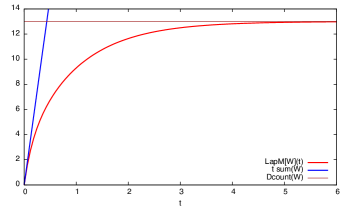
Figure 2. Data $W$ with 10 keys with $w_{x}=1$, 2 keys with $w_{x}=5$, and one key with $w_{x}=10$. The distinct count (number of keys) is $\operatorname{\textsf{Distinct}}(W)=13$ and the sum is $\operatorname{\textsf{Sum}}(W)=30$. We have $W(w)=10\delta(w-1)+2\delta(w-5)+\delta(w-10)$, where $\delta$ is Dirac Delta function. The transform (plotted) is $\operatorname{\mathcal{L}^{c}}[W](t)=10(1-e^{-t})+2(1-e^{-5t})+(1-e^{-10t})=13-10e^{-t}-2e^{-5t}-e^{-10t}$. The plot shows the asymptotes $t\operatorname{\textsf{Sum}}(W)$ for small $t$ and $\operatorname{\textsf{Distinct}}(W)$ for large $t$.

3. Laplace^c point measurements

We define a mapping function of elements such that the expectation of the (scaled) distinct count of output elements is equal to the Laplace^c transform $\operatorname{\mathcal{L}^{c}}[W](t)$ of $W$ at $t$. We also establish concentration around the expectation.

The basic element mapping is provided as Algorithm 1. A more efficient variant that performs computation proportional to the number of generated output elements is provided in Appendix A.

The mapping is parametrized by $t$ and by an integer $r\geq 1$ and uses a set of functions $H_{i}$ for $i\in[r]$. All we need to assume here is that for all $i$ and keys $x$, $H_{i}(x)$ are (nearly) unique. This can be achieved by concatenating $x$ to a string representation of $i$: $H_{i}(x)\equiv x\cdot\text{str}(i))$. To obtain output key representation that is logarithmic in $r\operatorname{\textsf{Distinct}}(W)$, we can apply a random hash function to the concatenated string. An element $e$ is processed by drawing a set of $r$ independent exponential random variables $y_{i}\sim\textsf{Exp}[\text{\em{e.value}}]$ with parameter e.value. For each $i$ such that $y_{i}<t$, the output key $H_{i}(\text{\em{e.key}})$ is created. Note that the number of output keys returned is between 0 and $r$.

Input: Element $e=(\text{\em{e.key}},\text{\em{e.value}})$, $t>0$, integer $r\geq 1$, hash functions $H_{i}$ $i\in[r]$

Output: A set OutKeys of at most $r$ outkeys

$\textnormal{{OutKeys}}\leftarrow[]$ // initialize

foreach $i\in[r]$ do

      $y_{i}\sim\textsf{Exp}[\text{\em{e.value}}]$ // independent exponentially distributed with parameter e.value

       if $y_{i}\leq t$ then

            $\textnormal{{OutKeys}}.append(H_{i}(\text{\em{e.key}}))$ // Append $H_{i}(\text{\em{e.key}})$ to list of output keys

            

      

return OutKeys

Algorithm 1 $\textnormal{{OutKeys}}_{t,H}(e)$: Map input element to outkeys

Our point measurement is

(11) $$\widehat{\operatorname{\mathcal{L}^{c}}}[W](t)=\frac{1}{r}\operatorname{\textsf{Distinct}}\left(\bigcup_{e}\text{\sc{OutKeys}}_{t,H}(e)\right)\ ,$$

which is number of distinct output keys generated for all data elements, divided by $r$. We now show that for any choice of $r\geq 1$, $t$, and input data $W$, the expectation of the measurement $\widehat{\operatorname{\mathcal{L}^{c}}}[W](t)$ is equal to the value of the Laplace^c transform of $W$ at $t$.

Lemma 3.1.

$$\textsf{E}[\widehat{\operatorname{\mathcal{L}^{c}}}[W](t)]=\operatorname{\mathcal{L}^{c}}[W](t)$$

Proof.

The distinct count of outkeys $r\widehat{\operatorname{\mathcal{L}^{c}}}[W](t)$ can be expressed as the sum of $rn$ Poisson trials. Each Poisson trial corresponds to “appearance at least once” of the potential outkey $H_{i}(x)$ over the $n=\operatorname{\textsf{Distinct}}(W)$ active input keys and $i\in[r]$. For each $i\in[r]$ and key $a$, the outkey $H_{i}(a)$ appears if the minimum $\textsf{Exp}[\text{\em{e.value}}]$ draw over elements $e$ with key $a$ is at most $t$. The minimum of these exponential random variables is exponentially distributed with parameter equal to their sum $w_{a}=\sum_{e\mid\text{\em{e.key}}=a}\text{\em{e.value}}$. This distribution has density function $w\exp(-wx)$. Therefore, the probability of the event is

(12) $$p(w_{a},t)=\int_{0}^{t}w_{a}\exp(-w_{a}y)dy=1-\exp(-w_{a}t)\ .$$

It follows that the expected contribution of a key $a$ with weight $w_{a}$ to the sum measurement is $rp(w_{a},t)$. Therefore the expected value of the measurement is

$$\textsf{E}[\widehat{\operatorname{\mathcal{L}^{c}}}[w](t)]=\frac{1}{r}\int_{0}^{\infty}W(w)rp(w,t)dw\equiv\operatorname{\mathcal{L}^{c}}[W](t)\ .$$

∎

Note that for $t=+\infty$, which corresponds to distinct counting, $p(w,t)=1$, and the measurement is always equal to its expectation $n$. More generally, $p(w,t)<1$ and we can bound the relative error by a straightforward application of Chernoff bound:

Lemma 3.2.

For $\delta<1$,

$$\Pr[\frac{|\widehat{\operatorname{\mathcal{L}^{c}}}[W](t)-\operatorname{\mathcal{L}^{c}}[W](t)|}{\operatorname{\mathcal{L}^{c}}[W](t)}\geq\delta]\leq 2\exp(-r\delta^{2}\operatorname{\mathcal{L}^{c}}[W](t)/3)\ .$$

Proof.

We apply Chernoff bounds to bound the deviation of the sum $r\widehat{\operatorname{\mathcal{L}^{c}}}[W](t)$ of our $rn$ independent Poisson random variables from its expectation $r\operatorname{\mathcal{L}^{c}}[W](t)$.

$$\Pr[\frac{|\widehat{\operatorname{\mathcal{L}^{c}}}[W](t)-\operatorname{\mathcal{L}^{c}}[w](t)|}{\operatorname{\mathcal{L}^{c}}[W](t)}\geq\delta]$$

$$= \Pr[|r\widehat{\operatorname{\mathcal{L}^{c}}}[W](t)-r\operatorname{\mathcal{L}^{c}}[W](t)|\geq\delta r\operatorname{\mathcal{L}^{c}}[W](t)]\ .$$

∎

The outkeys $E$ are processed by an approximate distinct counter and our final approximate measurement

(13) $$\widehat{\widehat{\operatorname{\mathcal{L}^{c}}}}[W](t)=\frac{1}{r}\widehat{\operatorname{\textsf{Distinct}}}(E)$$

is equal to the approximate count of distinct output keys divided by $r$. Since there are at most $r\operatorname{\textsf{Distinct}}(W)$ distinct output keys, the sketch size needed for CV $\epsilon$ is $O(\epsilon^{-2}+\log\log(r\operatorname{\textsf{Distinct}}(W)))=O(\epsilon^{-2}+\log\log\operatorname{\textsf{Distinct}}(W))$. Note that even a very large choice of $r$ will not significantly increase the sketch size. A large $r$, however, can affect the element mapping computation when there are many generated output elements.

We now consider the choice of $r$ that suffices for our quality guarantees. From Lemma 3.2, when

(14) $$r\operatorname{\mathcal{L}^{c}}[W](t)\geq 3\epsilon^{-2}$$

we have CV $\epsilon$ with tight concentration for $\widehat{\operatorname{\mathcal{L}^{c}}}[W](t)$ as an approximation of $\operatorname{\mathcal{L}^{c}}[W](t)$. Note that $r\operatorname{\mathcal{L}^{c}}[W](t)$ is the expected number of distinct output elements. We can combine the contributions to the error due to the measurement and its approximation, noting that the two are independent, and obtain that when (14) holds, the error of $\widehat{\widehat{\operatorname{\mathcal{L}^{c}}}}[W](t)$ as an approximation of $\operatorname{\mathcal{L}^{c}}[W](t)$ has CV $\sqrt{2}\epsilon$ and tight concentration.

We now provide a lower bound on $\operatorname{\mathcal{L}^{c}}[W](t)$ as a function of $t$.

Lemma 3.3.

$$\operatorname{\mathcal{L}^{c}}[W](t)\geq\frac{e-1}{e}\operatorname{\textsf{Sum}}(W)\min\{\frac{1}{\operatorname{\textsf{Max}}(W)},t\}\ ,$$

where $\operatorname{\textsf{Max}}(W)\equiv\max_{x}w_{x}$.

Proof.

From definition,

(15) $$\operatorname{\mathcal{L}^{c}}[W](t)\geq(1-\frac{1}{e})\sum_{x}\min\{1,tw_{x}\}$$

When $t\leq 1/\operatorname{\textsf{Max}}(W)$ we have $\sum_{x}\min\{1,tw_{x}\}=t\operatorname{\textsf{Sum}}(W)$. When $t\geq 1/\operatorname{\textsf{Max}}(W)$ we have $\sum_{x}\min\{1,tw_{x}\}\geq\operatorname{\textsf{Sum}}(W)$. ∎

The lemma implies that when $t\geq\sqrt{\epsilon}/\operatorname{\textsf{Max}}(W)$,

(16) $$r=\frac{e}{e-1}\epsilon^{-2.5}\frac{\operatorname{\textsf{Max}}(W)}{\operatorname{\textsf{Sum}}(W)}\leq\frac{e}{e-1}\epsilon^{-2.5}$$

always suffices to ensure that (14) holds.

Since we do not know $\operatorname{\textsf{Max}}(W)$ or $\operatorname{\textsf{Sum}}(W)$ in advance, we use the following strategy. Our approximate point measurement algorithm computes both an approximate sum $\widehat{\operatorname{\textsf{Sum}}}(W)$ and approximate count of output elements $\widehat{\operatorname{\textsf{Distinct}}(E)}$ generated by Algorithm 1 with $r$ as in (16). If $\widehat{\operatorname{\textsf{Distinct}}(E)}<3\epsilon^{-2}$, we return $t\widehat{\operatorname{\textsf{Sum}}}(W)$ and otherwise return (13).

We comment here that the choice of $r$ in (16) provides seamless worst-case quality guarantees for any $t$ and distribution $W$. In particular, having $t$ as small as $\sqrt{\epsilon}/\operatorname{\textsf{Max}}(W)$ and at the same time having $\operatorname{\textsf{Sum}}(W)=O(\operatorname{\textsf{Max}}(W))$. In practice, we may want to use a smaller value of $r$: While $r$ does not affect sketch size, it does affect element processing computation. The basic algorithm is linear in $r$. In Appendix A we provide a more efficient algorithm with computation that is linear in the number of generated output keys $O(r(1-\exp(-t\text{\em{e.value}}))$. We note that when $\operatorname{\textsf{Sum}}(W)\geq\epsilon^{-2.5}\operatorname{\textsf{Max}}(W)$ then $r=1$ suffices.

4. The soft capping span

The soft capping span $\overline{\widetilde{\textsf{cap}}}$ contains all functions $f$ that can be expressed as nonnegative linear combinations of $\widetilde{\textsf{cap}}_{T}$ functions. Equivalently, for some $a(t)\geq 0$,

(17) $$f(w)=\operatorname{\mathcal{L}^{c}}[a](w)=\int_{0}^{\infty}a(t)(1-e^{-wt})dt\ .$$

Note that $a(t)$ is the inverse Laplace^c transform of $f(w)$:

(18) $$a(t)=(\operatorname{\mathcal{L}^{c}})^{-1}[f(w)](t)\ .$$

The following is immediate from the definition (17)

Lemma 4.1.

For any well defined $f(w)$, $\int_{0}^{1}a(t)tdt<\infty$ and $\int_{1}^{\infty}a(t)dt<\infty$.

The soft capping span includes basic functions such as $\widetilde{\textsf{cap}}_{T}(w)$ for all $T>0$, $w^{p}$ for all $p\in(0,1)$, and $\ln(1+w)$. Explicit expressions for the inverse $\operatorname{\mathcal{L}^{c}}$ transforms of these functions are provided in Table 1. The table also lists other expressions that we will use for sketching the statistics. The derivations are established in Appendix B.

Table 1. Inverse $\operatorname{\mathcal{L}^{c}}$ transform of basic functions

$f(w)$	$a(t)=(\operatorname{\mathcal{L}^{c}})^{-1}[f(w)](t)$	$\int_{\tau}^{\infty}a(t)dt$	$\int_{0}^{\tau}a(t)tdt$
$\widetilde{\textsf{cap}}_{T}(w)$	$T\delta_{1/T}(t)$	$T$, when $y\leq 1/T$; $0$ otherwise	$0$ when $\tau<1/T$
$w^{p}$ ($p\in(0,1)$)	$\frac{p}{\Gamma(1-p)}t^{-(1+p)}$	$\frac{1}{\tau^{p}\Gamma(1-p)}$	$\frac{p}{(1-p)\Gamma(1-p)}\tau^{1-p}$
$\sqrt{w}$	$\frac{1}{2\sqrt{\pi}}t^{-1.5}$	$\frac{1}{\sqrt{\pi\tau}}$	$\frac{\tau^{0.5}}{\sqrt{\pi}}$
$\log(1+w)$	$\frac{e^{-t}}{t}$	$\int_{\tau}^{\infty}\frac{e^{-t}}{t}dt=-\tau\text{Ei}(-\tau)$	$1-e^{-\tau}$

We can express $f(W)$ in terms of the inverse $\operatorname{\mathcal{L}^{c}}$ transform $a(t)$ of $f(w)$ and the transform $\operatorname{\mathcal{L}^{c}}[W]$ of the frequencies:

(19) $$f(W) = \int_{0}^{\infty}f(w)W(w)dw$$

$$= \int_{0}^{\infty}W(w)\operatorname{\mathcal{L}^{c}}[a](w)dw$$

$$= \int_{0}^{\infty}a(t)\int_{0}^{\infty}W(w)(1-e^{-wt})dwdt$$

$$= \int_{0}^{\infty}a(t)\operatorname{\mathcal{L}^{c}}[W](t)dt\ .$$

Alternatively, when the inverse transform has a discrete form, that is, when we can express $f$ using $\{a_{t}\}$ for $t\in Y$ as

(20) $$f(w)=\sum_{t\in Y}a_{t}(1-e^{-wt})\ ,$$

(Equivalently, $a(t)$ is a linear combination of Dirac delta functions at $t\in Y$). We can express $f(W)$ in terms of corresponding points of $\operatorname{\mathcal{L}^{c}}[W]$:

$$f(W)=\sum_{t\in Y}a_{t}\operatorname{\mathcal{L}^{c}}[W](t)\ .$$

We will find it convenient to work with the notation:

(21) $$\operatorname{\mathcal{L}^{c}}[W][a]_{\tau}^{b}\equiv\int_{\tau}^{b}a(t)\operatorname{\mathcal{L}^{c}}[W](t)dt\ .$$

When the subscript or superscript are omitted, we use the defaults $\tau=0$ and $b=\infty$. With approximate $\operatorname{\mathcal{L}^{c}}$ measurements we have

(22) $$\widehat{\widehat{\operatorname{\mathcal{L}^{c}}}}[W][a]_{\tau}^{b}=\int_{\tau}^{b}a(t)\widehat{\widehat{\operatorname{\mathcal{L}^{c}}}}[W](t)dt\ .$$

When $f(w)$ is such that the inverse $\operatorname{\mathcal{L}^{c}}$ transform $a(t)$ is a sum of Dirac delta functions, we can approximate $f(W)$ using corresponding point measurements of $\operatorname{\mathcal{L}^{c}}[W]$. In the next section we introduce combination $\operatorname{\mathcal{L}^{c}}$ measurements which allow us to approximate $\operatorname{\mathcal{L}^{c}}[W][a]$ for any nonnegative continuous $a(t)\geq 0$.

5. Combination $\operatorname{\mathcal{L}^{c}}$ measurements

In this section we show how to sketch $\operatorname{\mathcal{L}^{c}}[W][a]_{0}^{\infty}$ for any $a(t)\geq 0$ that satisfies the conditions in Lemma 4.1. Recall that his allows us to sketch any $f(W)\in\overline{\widetilde{\textsf{cap}}}$ (see Section 4).

We define randomized mapping functions of elements, tailored to some $a(t)\geq 0$ and $\tau>0$, such that the expectation of the (scaled) max-distinct statistics of output elements is equal to $\operatorname{\mathcal{L}^{c}}[W][a]_{\tau}^{\infty}$ (see notation (21)) we also establish concentration around the expectation. We then estimate the component $\operatorname{\mathcal{L}^{c}}[W][a]_{0}^{\tau}$ separately through $\widehat{\operatorname{\textsf{Sum}}}(W)$.

5.1. Element mapping

Consider $a(t)\geq 0$. Our element processing is a simple modification of the element processing Algorithm 1. The algorithm inputs the function $a()$ (instead of $t$) and returns output elements (outkey and value pairs) instead of only returning outkeys. Pseudocode is provided as Algorithm 2.

Input: Element $e=(\text{\em{e.key}},\text{\em{e.value}})$, $a(t)\geq 0$, integer $r\geq 1$, hash functions $H_{i}$ $i\in[r]$, $\tau>0$

Output: OutElements: A set of at most $r$ output elements

$\textnormal{{OutElements}}\leftarrow[]$

foreach $i\in[r]$ do

      $y_{i}\sim\textsf{Exp}[\text{\em{e.value}}]$ // independent exponentially distributed with parameter e.value

       $v\leftarrow\int_{\max\{\tau,y_{i}\}}^{\infty}a(t)dt$

       if $v>0$ then

            $\textnormal{{OutElements}}.append((H_{i}(\text{\em{e.key}}),v))$ // New output element

            

      

return OutElements

Algorithm 2 OutElements ${}_{a,H}(e)$: Map of element $e$ to a set of output elements for a $\operatorname{\mathcal{L}^{c}}[W][a]_{\tau}^{\infty}$ measurement

We show that the max-distinct statistics of the output elements divided by $r$

(23) $$\widehat{\operatorname{\mathcal{L}^{c}}[W][a]}_{\tau}^{\infty}=\frac{1}{r}\operatorname{\textsf{MxDistinct}}\left(\bigcup_{e\in W}\textnormal{{OutElements}}_{a}(e)\right)\$$

has expectation equal to $\operatorname{\mathcal{L}^{c}}[W][a]_{\tau}^{\infty}$ with good concentration:

Lemma 5.1.

$$\textsf{E}[\widehat{\operatorname{\mathcal{L}^{c}}[W][a]}_{\tau}^{\infty}]=\operatorname{\mathcal{L}^{c}}[W][a]_{\tau}^{\infty}$$

$$\forall\delta<1,\,\Pr[\frac{|\widehat{\operatorname{\mathcal{L}^{c}}[W][a]}_{\tau}^{\infty}-\operatorname{\mathcal{L}^{c}}[W][a]_{\tau}^{\infty}}{\operatorname{\mathcal{L}^{c}}[W][a]_{\tau}^{\infty}}\geq\delta]$$

$$\leq 2\exp(-r\delta^{2}\operatorname{\mathcal{L}^{c}}[W][\tau]/3)\ .$$

Proof.

The claim on the expectation follows from linearity of expectation and the claim for point measurements for each $t$ in Lemma 3.1. The concentration follows from Lemma 3.2 which establishes point-wise concentration at each $t$, combined with the relation

$$\min_{t\in[\tau,\infty)}\operatorname{\mathcal{L}^{c}}[W](t)=\operatorname{\mathcal{L}^{c}}[W](\tau)\$$

which follows from monotonicity of $\operatorname{\mathcal{L}^{c}}[W](t)$. ∎

Note that the assumption $a(t)\geq 0$ is necessary for correctness. It ensures monotonicity of $\int_{y}^{\infty}a(t)dt$ in $y$ which implies that the maximum indeed corresponds to minimum $y$.

We now address quality of approximation. From the lemma, quality is bounded by a function of $\operatorname{\mathcal{L}^{c}}[W](\tau)$. Using our treatment of point measurements, we know that it suffices to ensure that $\tau$ and $r$ are large enough so that (14) holds. As with point measurements, we can use $\tau=\sqrt{\epsilon}/\operatorname{\textsf{Max}}(W))$ and $r$ as in (16) to obtain a concentrated measurement of $\operatorname{\mathcal{L}^{c}}[W][a]_{\tau}^{\infty}$.

To obtain an estimate of $\operatorname{\mathcal{L}^{c}}[W][a]_{0}^{\infty}$, we need to separately estimate $\operatorname{\mathcal{L}^{c}}[W][a]_{0}^{\tau}$. From Lemma 2.1, when $\tau\leq\sqrt{\epsilon}/\operatorname{\textsf{Max}}(W)$, we have

(24) $$\operatorname{\mathcal{L}^{c}}[W][a]_{0}^{\tau}\approx\int_{0}^{\tau}a(t)t\operatorname{\textsf{Sum}}(W)dt\approx\widehat{\operatorname{\textsf{Sum}}(W)}\int_{0}^{\tau}a(t)tdt\ .$$

Closed expressions for $\int_{0}^{\tau}a(t)tdt$ (used in (24) and for $\int_{\tau}^{\infty}a(t)dt$ (used in Algorithm 2) for inverse transforms of basic functions are provided in Table 1. Note that these expressions are bounded and well defined for all $a$ that are inverse $\operatorname{\mathcal{L}^{c}}$ transform of a $\overline{\widetilde{\textsf{cap}}}$ function (see Lemma B.2).

Our sketch consists of a $\widehat{\operatorname{\textsf{Sum}}}$ sketch applied to data elements $W$ and a $\widehat{\operatorname{\textsf{MxDistinct}}}$ sketch applied to output element $E$ produced by applying the element mapping Algorithm 2 to $W$. The final estimate we return is

(25) $$\widehat{\widehat{\operatorname{\mathcal{L}^{c}}}}[W][a]_{0}^{\infty}=\frac{1}{r}\widehat{\operatorname{\textsf{MxDistinct}}}(E)+\widehat{\operatorname{\textsf{Sum}}}(W)\int_{0}^{\tau}a(t)tdt\ .$$

There is one subtlety here that was deferred for the sake of exposition: We do not know $\operatorname{\textsf{Max}}(W)$ and therefore can not simply set $\tau$ prior to running the algorithm. To obtain the worst-case bound we set $r$ as in (16) and set $\tau$ adaptively to be the $\ell=3\epsilon^{-2}$ smallest $y$ value generated for a distinct output key. To do so, we extend our sketch to include another component, a “sidelined” set, which is the $\ell$ distinct output keys with smallest $y$ values processed so far. Note that this sketch component is also composable. The sidelined elements are not immediately processed by the $\operatorname{\textsf{MxDistinct}}$ sketch: The processing is delayed to when they are not sidelined, that is, to the point that due to merges or new arrivals, there are $\ell$ other distinct output keys with lower $y$ values. Finally, when the sketches are used to extract an estimate of the statistics, we set $\tau$ as the largest $y$ in the sidelined set, feed all the sidelined keys to the $\operatorname{\textsf{MxDistinct}}$ sketch with value $\int_{\tau}^{\infty}a(t)dt$, and apply the estimator (25). Note that explicitly maintaining the sidelined output keys and $y$ value pairs requires $\epsilon^{-2}\log n$ storage. Details on doing so in double logarithmic size are outlined in Section C.1.

5.2. Max-distinct sketches

Popular composable weighted sampling schemes such as the with-replacement $k$-mins samples and the without-replacement bottom-$k$ samples (Rosen1972:successive, ; Rosen1997a, ; bottomk07:ds, ; bottomk:VLDB2008, ) naturally extend to data elements with non-unique keys where the weight $m_{x}$ of the key $x$ is interpreted as the maximum value of an element with key $x$. A bottom-$k$ sample over elements with unique keys is (Rosen1972:successive, ) computed by drawing for each element an independent random rank value that is exponentially distributed with parameter e.value $r_{e}\sim\textsf{Exp}[\text{\em{e.value}}]$. The sample includes the $k$ distinct keys with minimum $r_{e}$ and the corresponding $m_{x}$. It is easy to see that this sampling scheme can be carried out using composable sketches that stores $k=\epsilon^{-2}$ key value pairs. For max-distinct statistics we instead use the ranks $r_{e}=-\ln u_{\text{\em{e.key}}}/\text{\em{e.value}}$, where $u_{\text{\em{e.key}}}\sim U[0,1]$ is a hash function that maps keys to independent uniform random numbers. These ranks are exponentially distributed, but consistent for the same key so that the minimum rank of a key is exponentially distributed with parameter equal to $m_{x}$. We can apply an estimator to this sample to obtain an estimate of the max-distinct statistics of the data with CV $1/\sqrt{k-2}\approx\epsilon$. Through technical use of offsets and randomized rounding and using with-replacement sampling we can design max-distinct sketches of size $O(\log\log n+\epsilon^{-2}\log\epsilon^{-1})$ (assuming $1\leq m_{x}=O(\text{poly}(n))$.) The design relates to MinHash sketches with base-$b$ ranks (ECohenADS:TKDE2015, ) and is detailed in Section C.

6. Full range $\operatorname{\mathcal{L}^{c}}$ measurements

We consider now computing approximations of the transform $\operatorname{\mathcal{L}^{c}}[W](t)$ for all $t$, which we refer to as a full range measurement. This is a representation of a function that returns “coordinated” $\operatorname{\mathcal{L}^{c}}[W](t)$ measurements for any $t$ value. Our motivation is that an approximate full-range measurement of $W$ provides us with estimates of the statistics $f(W)$ for any $f\in\overline{\widetilde{\textsf{cap}}}$.

Concretely, consider the set of output keys $\textnormal{{OutKeys}}_{t,H}(e)$ generated by Algorithm 1 for input element $e$ when fixing the parameter $r$, the set of hash functions $\{H_{i}\}$, and the randomization $\{y_{i}\}$, but varying $t$. It is easy to see that the set $\textnormal{{OutKeys}}_{t}(e)$ monotonically increases with $t$ until it reaches size $r$. We can now consider all outkeys generated for input $W$ as a function of $t$

$$\textnormal{{OutKeys}}_{t}(W)\equiv\bigcup_{e\in W}\textnormal{{OutKeys}}_{t}(e)\ .$$

The number of distinct outkeys increases with $t$ until it reaches size $rn$, where $n$ is the number of distinct input keys. Our full-range measurement is accordingly defined as the function

(26) $$\widehat{\operatorname{\mathcal{L}^{c}}}[W](t)=\frac{1}{r}\bigg{|}\textnormal{{OutKeys}}_{t}(W)\bigg{|}\ .$$

Equivalently, this can be expressed through the element mapping provided as Algorithm 3. For each input element $e$, the algorithm generates $r$ output elements $\textnormal{{OutElements}}_{H}(e)$ that are outkey and value pairs. We denote the set of output elements generated for all input elements by $\textnormal{{OutElements}}(W)$. We then have

(27) $$\widehat{\operatorname{\mathcal{L}^{c}}}[W](t)=\frac{1}{r}\operatorname{\textsf{Distinct}}\{e\in\textnormal{{OutElements}}(W)\mid\text{\em{e.value}}\leq t\}\ .$$

The number of distinct keys in output elements that have value at most $t$. Note that as with point measurements, for the regime of $t$ values where $|\textnormal{{OutKeys}}_{t}(W)|\leq 3\epsilon^{-2}$, we use instead $\widehat{\operatorname{\mathcal{L}^{c}}}[W](t)\approx t\operatorname{\textsf{Sum}}(W)$.

We can also define a combination measurement obtained from a full range measurement as

$$\widehat{\operatorname{\mathcal{L}^{c}}}[W][a]=\int_{0}^{\infty}a(t)\widehat{\operatorname{\mathcal{L}^{c}}}[W](t)dt\ .$$

We show that this formulation is equivalent to directly obtaining a combination measurement:

Corollary 6.1.

Lemma 5.1 also applies to $\widehat{\operatorname{\mathcal{L}^{c}}[W][a]}$ computed from a full-range measurement

Proof.

Consider element mappings for full-range and combination measurements that are performed using the same randomization (hash functions $H$ and draws $y$). Consider the combination measurement computed from $|\textnormal{{OutKeys}}_{t}(W)|$. It is easy to verify that

$$\widehat{\operatorname{\mathcal{L}^{c}}[W][a]} = \frac{1}{r}\operatorname{\textsf{MxDistinct}}\left(\bigcup_{e\in W}\textnormal{{OutElements}}_{a}(e)\right)$$

$$= \frac{1}{r}\int_{0}^{\infty}a(t)|\textnormal{{OutKeys}}_{t}(W)|dt\ .$$

∎

We next discuss composable all-threshold distinct counting sketch that when applied to $\textnormal{{OutElements}}(W)$ allow us to obtain an approximate point measurement of $\widehat{\widehat{\operatorname{\mathcal{L}^{c}}}}[W](t)$ for any $t$ or compute an approximate combination measurement $\widehat{\widehat{\operatorname{\mathcal{L}^{c}}}}[W][a]$ for any $a\in\operatorname{\mathcal{L}^{c}}^{-1}(\overline{\widetilde{\textsf{cap}}})$.

Input: Element $e=(\text{\em{e.key}},\text{\em{e.value}})$, integer $r\geq 1$, hash functions $\{H_{i}\}$ $i\in[r]$

Output: OutElements: A set of $r$ output elements

$\textnormal{{OutElements}}\leftarrow[]$

foreach $i\in[r]$ do

      $y_{i}\sim\textsf{Exp}[\text{\em{e.value}}]$ // independent exponentially distributed with parameter e.value

       $\textnormal{{OutElements}}.append((H_{i}(\text{\em{e.key}}),y_{i}))$ // New output element

      

return OutElements

Algorithm 3 OutElements ${}_{\{H_{i}\}}(e)$: Map of element $e$ to a set of output elements for full range measurement

An all-threshold sketch of a set $E$ of key value pairs is a composable summary structure which allows us to obtain an approximation $\widehat{\operatorname{\text{{\sf TDistinct}}}}_{t}(E)$ for any $t$ (see (6). The design mimics the extension of MinHash sketches to All-Distance Sketches (ECohen6f, ; ECohenADS:TKDE2015, ), noting that Hyperloglog sketches can be viewed as a degenerate form of MinHash sketches. Details are provided in Section E.

7. The “hard” Capping span

The capping transform expresses functions as nonnegative combinations of capping functions. The transform is interesting to us here because it allows us to extend approximations of capping statistics to the rich family of functions with a capping transform. We define the capping transform of a function $f$ as a function $a(t)\geq 0$ and $A_{\infty}\geq 0$ such that $\int_{0}^{\infty}a(t)dt<\infty$ and

$$f(x)=A_{\infty}x+\int_{0}^{\infty}a(t)\textsf{cap}_{t}(x)dt\ .$$

It is useful to allow the transform to include a discrete and continuous components, that is, have continuous $a(t)$ and a discrete set $\{A_{t}\}>0$ for $t\in Y$ such that

$$f(x)=A_{\infty}x+\sum_{t\in Y}A_{t}\textsf{cap}_{t}(x)+\int_{0}^{\infty}a(t)\textsf{cap}_{t}(x)dx\ ,$$

and require that $A_{\infty}+\sum_{t\in Y}A_{t}+\int_{0}^{\infty}a(t)dt<\infty$. For convenience, however we will use a single continuous transform $a()$ but allow it to include a linear combination of Dirac delta functions at points $Y$. The one exception is the coefficient $A_{\infty}<\infty$ of $\textsf{cap}_{\infty}(x)=x$ which is separate.

We denote by $\overline{\textsf{cap}}$ the set of functions with a capping transform. We can characterize this set of functions as follows:

Theorem 7.1.

Let $f:[0,\infty]$ be a nonnegative, continuous, concave, and monotone non-decreasing function such that $f(0)=0$ and $\partial_{+}f(0)<\infty$. Then $f\in\overline{\textsf{cap}}$ with the capping transform:

(30) $$a(x) = \left\{\begin{array}[]{ll}-\partial^{2}f(x)&\text{ when }\,\partial^{2}_{-}f(x)=\partial^{2}_{+}f(x)\\ (\partial_{-}f(x)-\partial_{+}f(x))\delta_{x}&\text{otherwise}\end{array}\right.$$

(31) $$A_{\infty} = \partial f(\infty)$$

where $\delta$ is the Dirac delta function and $\partial f(\infty)\equiv\lim_{t\rightarrow\infty}\partial f(t)$.

Proof.

From monotonicity, $f$ is differentiable almost everywhere and the left and right derivatives $\partial_{+}f(x)$ and $\partial_{-}f(x)$ are well defined. Because $f$ is continuous and monotone, we have

(32) $$f(w)=\int_{0}^{w}\partial_{+}f(t)dt=\int_{0}^{w}\partial_{-}f(t)\equiv\int_{0}^{w}\partial f(t)dt\ .$$

From concavity, for all $x\leq y$, $\partial_{+}f(y)\leq\partial_{-}f(x)$. In particular the slope of $\partial f(x)$ is initially (sub)linear and can only decrease as $x$ decreases. In particular the limit $\partial f(\infty)\geq 0$ is well defined.

Since $\partial f(x)$ is monotone, it is differentiable and equality holds almost everywhere:

$$\partial^{2}_{+}f(x)=\partial^{2}_{-}f(x)\equiv\partial^{2}f(x)\ .$$

From concavity, we have $\partial^{2}_{+}f(x),\partial^{2}_{-}f(x)\leq 0$.

Note that at all $w$ with well defined $\partial f(w)$, we have

(33) $$\partial f(w)=\partial_{+}f(0)-\int_{0}^{w}a(t)dt\ .$$

In particular, when taking the limit as $w\rightarrow\infty$ we get

(34) $$A_{\infty}+\int_{0}^{\infty}a(t)dt=\partial_{+}f(0)\ .$$

$$\int_{0}^{\infty}a(t)\textsf{cap}_{t}(w)dt$$

$$= \int_{0}^{\infty}a(t)\min\{t,w\}dt$$

(36) $$= \int_{0}^{w}ta(t)dt+w\int_{w}^{\infty}a(t)dt$$

(37) $$= w\int_{0}^{w}a(t)dt-\int_{0}^{w}(\partial_{+}f(0)-\partial f(t))dt+w\int_{w}^{\infty}a(t)dt$$

(38) $$= w\int_{0}^{\infty}a(t)dt+f(w)-w\partial_{+}f(0)$$

(39) $$= f(w)-A_{\infty}w$$

Derivation (36) uses the definition of $\textsf{cap}_{t}$, (37) uses integration by parts and (33), (38) uses (32), and finally (39) uses (34). ∎

The capping transforms of some example functions are derived below and summarized in Table 2. Note that the transform is a linear operator, so the transform of a linear combination is a corresponding linear combination of the transforms.

• $f(w)=\textsf{cap}_{T}(w)$ has the transform $A_{\infty}=0$ and $a(x)=\delta_{T}(x)$.

• $f(w)=w=\textsf{cap}_{\infty}(w)$ has the transform $A_{\infty}=1$, $a(x)=0$ for all $x$.

• Moments $f(w)=w^{p}$ for $p\in(0,1)$. Here we assume that $w\geq 1$ and for convenient replace the function with a linear segment $f(w)=\min\{w,w^{p}\}$ at the interval $w\in[0,1]$. Note that the modified moment function satisfies the requirements of Theorem (7.1). We have $\partial f(w)=1$, $\partial^{2}f(w)=0$ for $w<1$ and $\partial f(w)=pw^{p-1}$ and $\partial^{2}f(w)=p(p-1)w^{p-2}$ when $w\geq 1$. Note that $\partial f(\infty)=0$ and $\partial_{+}f(0)=1$.

  We obtain $A_{\infty}=0$, $a(x)=p(1-p)x^{p-2}$ for $x>1$ and $a(1)=(1-p)\delta_{1}$.

• Soft capping $f(w)=\widetilde{\textsf{cap}}_{T}(w)=T(1-e^{-w/T})$. We have $\partial f(w)=e^{-w/T}$ and $\partial^{2}f(w)=-\frac{1}{T}e^{-w/T}$. Note that $\partial f(\infty)=0$ and $\partial_{+}f(0)=1$.

  We obtain $A_{\infty}=0$ and $a(x)=\frac{1}{T}e^{-x/T}$.

Table 2. Example capping transforms

$f(w)$	capping transform
$\textsf{cap}_{T}(w)$	$A_{\infty}=0$, $a(x)=\delta_{T}(x)$
$w$	$A_{\infty}=1$, $a(x)=0$
$\min\{w,w^{p}\}$	$A_{\infty}=0$, $a(x)=p(1-p)x^{p-2}$ for $x>1$,
	$a(x)=0$ for $x<1$, $a(1)=(1-p)\delta_{1}$
$\widetilde{\textsf{cap}}_{T}(w)$	$A_{\infty}=0$, $a(x)=\frac{1}{T}e^{-x/T}$
$\log(1+w)$	$A_{\infty}=0$, $a(x)=\frac{1}{(1+x)^{2}}$

7.1. Sketching with signed inverse transforms

We now consider sketching $f$-statistics that are not in $\overline{\widetilde{\textsf{cap}}}$ but where $f$ has a signed inverse transform $a(t)=\operatorname{\mathcal{L}^{c}}^{-1}[f(w)](t)$ (17). We use the notation $a(t)=a_{+}(t)-a_{-}(t)$ where

(40) $$a_{+}(t)=\max\{a(t),0\}\,\text{ and }\,a_{-}(t)=\max\{-a(t),0\}\ .$$

We define $f_{+}(w)=\operatorname{\mathcal{L}^{c}}[a_{+}](w)$ and $f_{-}(w)=\operatorname{\mathcal{L}^{c}}[a_{-}](w)$. Note that for all $w$, $f(w)=f_{+}(w)-f_{-}(w)$ and in particular $f(W)=f_{+}(W)-f_{-}(W)$. Since $a_{+},a_{-}\geq 0$, we can obtain a good approximations $\hat{f}_{+}(W)$ and $\hat{f}_{-}(W)$ for each of $f_{+}(W)=\operatorname{\mathcal{L}^{c}}[W][a_{+}]$ and $f_{-}(W)=\operatorname{\mathcal{L}^{c}}[W][a_{-}]$ using approximate full-range, two combination, or several point measurements when $a$ is discrete and small. We approximate $f(W)$ using the difference $\hat{f}(W)=\hat{f}_{+}(W)-\hat{f}_{-}(W)$.

The quality of this estimate depends on a parameter $\rho$:

(41) $$\rho(a)\equiv\max_{w}\max\frac{\operatorname{\mathcal{L}^{c}}[a_{+}](w)}{\operatorname{\mathcal{L}^{c}}[a](w)},\frac{\operatorname{\mathcal{L}^{c}}[a_{-}](w)}{\operatorname{\mathcal{L}^{c}}[a](w)}$$

Lemma 7.2.

For all $W$, $f(w)=\operatorname{\mathcal{L}^{c}}[a](w)$,

$$\frac{|f(W)-\hat{f}(W)|}{f(W)}\leq$$

$$\rho(a)\left(\frac{|\operatorname{\mathcal{L}^{c}}[W][a_{+}]-\widehat{\operatorname{\mathcal{L}^{c}}}[W][a_{+}]|}{\operatorname{\mathcal{L}^{c}}[W][a_{+}]}\ +\frac{|\operatorname{\mathcal{L}^{c}}[W][a_{-}]-\widehat{\operatorname{\mathcal{L}^{c}}}[W][a_{-}]|}{\operatorname{\mathcal{L}^{c}}[W][a_{-}]}\ \right)$$

Proof.

We use $\hat{f}(W)=\widehat{\operatorname{\mathcal{L}^{c}}}[W][a_{+}]-\widehat{\operatorname{\mathcal{L}^{c}}}[W][a_{-}]$ and $f(W)=\operatorname{\mathcal{L}^{c}}[W][a_{+}]-\operatorname{\mathcal{L}^{c}}[W][a_{-}]$. Also note that using the definition of $\rho$, for all $W$,

$$f(W) = \int_{0}^{\infty}W(w)\operatorname{\mathcal{L}^{c}}[a](w)dw$$

$$\geq \int_{0}^{\infty}W(w)\frac{\operatorname{\mathcal{L}^{c}}[a]_{+}(w)}{\rho(a)}dw$$

$$= \frac{1}{\rho(a)}\int_{0}^{\infty}W(w)\operatorname{\mathcal{L}^{c}}[a]_{+}(w)dw=f_{+}(W)\ .$$

Symmetrically, for all $W$, $\rho f(W)\geq f_{-}(W)$.

Combining it all we obtain

$$\frac{|\hat{f}(W)-f(W)|}{f(W)}=$$

$$\frac{\widehat{\operatorname{\mathcal{L}^{c}}}[W][a_{+}]-\operatorname{\mathcal{L}^{c}}[W][a_{+}]}{f(W)}+\frac{\widehat{\operatorname{\mathcal{L}^{c}}}[W][a_{-}]-\operatorname{\mathcal{L}^{c}}[W][a_{-}]}{f(W)}$$

$$\leq \rho(a)\frac{|\widehat{\operatorname{\mathcal{L}^{c}}}[W][a_{+}]-\operatorname{\mathcal{L}^{c}}[W][a_{+}]|}{\operatorname{\mathcal{L}^{c}}[W][a_{+}]}+\rho(a)\frac{|\widehat{\operatorname{\mathcal{L}^{c}}}[W][a_{-}]-\operatorname{\mathcal{L}^{c}}[W][a_{-}]|}{\operatorname{\mathcal{L}^{c}}[W][a_{-}]}$$

∎

That is, when the components $f_{+}(W)$ and $f_{-}(W)$ are estimated within relative error $\epsilon$, then our estimate of $f(W)$ has relative error at most $\epsilon\rho$. In particular, the concentration bound in Lemma 5.1 holds with $\rho\delta$ replacing $\delta$ and the sketch size has $\epsilon\rho$ replacing $\epsilon$.

When the exact inverse transform $a$ of $f$ is not defined or has a large $\rho(a)$, we look for an approximate inverse transform $a$ such that $\rho(a)$ is small and $f(w)\approx\operatorname{\mathcal{L}^{c}}[a](w)$:

(42) $$\textsf{relerr}(f,\operatorname{\mathcal{L}^{c}}[a])=\max_{w>0}\frac{|f(w)-\operatorname{\mathcal{L}^{c}}[a](w)|}{f(w)}\leq\epsilon$$

We will apply this approach to approximate hard capping functions. In general, fitting data or functions to sums of exponentials is a well-studied problem in applied math and numerical analysis. Methods often have stability issues. A method of choice is the Varpro (Variable projection) algorithm of Golub and Pereyra (varpro_Golub:SiNumAs1973, ) and improvements (varpro2013, ) which has Matlab and SciPy implementation.

7.2. From $\textsf{cap}_{1}$ to $\overline{\textsf{cap}}$

We show that from an approximate signed inverse transform of $\textsf{cap}_{1}$ we can obtain one with the same quality for any $f\in\overline{\textsf{cap}}$. We first consider the special case of $\textsf{cap}_{T}$ functions:

Lemma 7.3.

Let $\alpha$ be such that $\operatorname{\mathcal{L}^{c}}[\alpha]$ is an approximation of $\textsf{cap}_{1}$. Then for all $T$, $\operatorname{\mathcal{L}^{c}}[\alpha_{T}]$, where $\alpha_{T}(x)\equiv\alpha(x/T)$ is a corresponding approximation of $\textsf{cap}_{T}$. That is,

$$\textsf{relerr}(\textsf{cap}_{T},\operatorname{\mathcal{L}^{c}}[\alpha_{T}]) = \textsf{relerr}(\textsf{cap}_{1},\operatorname{\mathcal{L}^{c}}[\alpha])$$

$$\rho(\alpha_{T}) = \rho(\alpha)\ .$$

Proof.

The claim on relerr and $\rho$ follows from the pointwise equality

(43) $$\frac{|\textsf{cap}_{T}(w)-\operatorname{\mathcal{L}^{c}}[\alpha_{T}](w)|}{\textsf{cap}_{T}(w)}=\frac{|\textsf{cap}_{1}(w/T)-\operatorname{\mathcal{L}^{c}}[\alpha](w/T)|}{\textsf{cap}_{1}(w/T)}\ .$$

For $\rho$ observe the correspondence

(44) $$\frac{\operatorname{\mathcal{L}^{c}}[\alpha_{T+}](w/T)}{\operatorname{\mathcal{L}^{c}}[\alpha_{T}](w/T)}=\frac{\operatorname{\mathcal{L}^{c}}[\alpha_{+}](w)}{\operatorname{\mathcal{L}^{c}}[\alpha](w)}$$

and similarly for $\alpha_{-}$. The maximum over $w$ of both sides is therefore the same. ∎

Theorem 7.4.

Let $f\in\overline{\textsf{cap}}$ and let $a(t)$ be the capping transform of $f$. Let $\alpha(x)$ be such that $\operatorname{\mathcal{L}^{c}}[\alpha](w)$ is an approximation of $\textsf{cap}_{1}$. Then

(45) $$c(x)=\int_{0}^{\infty}a(T)\alpha(x/T)dT\ ,$$

is an approximate inverse transform of $f$ that satisfies

(46) $$\rho(c) \leq \rho(\alpha)$$

(47) $$\textsf{relerr}(f,\operatorname{\mathcal{L}^{c}}[c]) \leq \textsf{relerr}(\textsf{cap}_{1},\operatorname{\mathcal{L}^{c}}[\alpha])$$

Proof.

Recall from Lemma 7.3, that for all $T$, $\textsf{cap}_{T}$ is approximated by $\operatorname{\mathcal{L}^{c}}[\alpha_{T}]$, where $\alpha_{T}(x)=\alpha(x/T)$). We have

$$f(w) = \int_{0}^{\infty}a(T)\textsf{cap}_{T}(w)dT$$

$$\hat{f}(w) = \int_{0}^{\infty}a(T)\operatorname{\mathcal{L}^{c}}[\alpha_{T}](w)dT$$

The approximation $\hat{f}$ is obtained by substituting respective approximations for the capping functions. For all $W$,

$$\textsf{relerr}(f(W),\hat{f}(W)) \leq \max_{w}\textsf{relerr}(\textsf{cap}_{T},\operatorname{\mathcal{L}^{c}}[\alpha_{T}])$$

$$= \textsf{relerr}(\textsf{cap}_{1},\operatorname{\mathcal{L}^{c}}[\alpha])\ .$$

The inequality follows from $a\geq 0$. The last equality follows from Lemma 7.3.

We now show that $\hat{f}(W)=\operatorname{\mathcal{L}^{c}}[c]$:

$$\hat{f}(w) = \int_{0}^{\infty}a(T)\operatorname{\mathcal{L}^{c}}[\alpha_{T}](w)dT$$

$$= \int_{0}^{\infty}\int_{0}^{\infty}a(T)\alpha_{T}(x)(1-e^{-wx})dxdT$$

$$= \int_{0}^{\infty}\int_{0}^{\infty}a(T)\alpha(x/T)dT(1-e^{-wx})dx$$

$$= \int_{0}^{\infty}c(x)(1-e^{-wx})dx=\operatorname{\mathcal{L}^{c}}[c]\ ,$$

where

$$c(x)=\int_{0}^{\infty}a(T)\alpha_{T}(x)dT=\int_{0}^{\infty}a(T)\alpha(x/T)dT\ .$$

We will now show that $\forall w,\ \operatorname{\mathcal{L}^{c}}[c_{+}](w)\leq\rho(\alpha)\operatorname{\mathcal{L}^{c}}[c](w)$. The claim for $c_{-}$ is symmetric and together using the definition of $\rho$ they imply that $\rho(c)\leq\rho(\alpha)$. We first observe that

$$c_{+}(x) = \max\{0,\int_{0}^{\infty}a(T)(\alpha_{T+}(x)-\alpha_{T-}(x)dT\}$$

$$= \max\{0,\int_{0}^{\infty}a(T)(\alpha_{T+}(x)dT-\int_{0}^{\infty}a(T)\alpha_{T-}(x)dT\}$$

$$\leq \int_{0}^{\infty}a(T)\alpha_{T+}(x)dT\ .$$

The last equality follows from the two integrals being nonnegative.

Therefore,

$$\operatorname{\mathcal{L}^{c}}[c_{+}](w) \leq \int_{0}^{\infty}a(T)\operatorname{\mathcal{L}^{c}}[\alpha_{T+}](w)dT$$

$$\leq \int_{0}^{\infty}a(T)\rho(\alpha_{T})\operatorname{\mathcal{L}^{c}}[\alpha_{T}](w)dT$$

$$= \rho(\alpha)\int_{0}^{\infty}a(T)\operatorname{\mathcal{L}^{c}}[\alpha_{T}](w)dT$$

$$= \rho(\alpha)\operatorname{\mathcal{L}^{c}}[c](w)\ .$$

Using Lemma 7.3 that established $\rho(\alpha)=\rho(\alpha_{T})$.

∎

It follows that to approximate $f(W)$ we do as follows. We compute the capping transform of $f$ and use an approximate inverse transform of $\textsf{cap}_{1}$, from which we obtain an approximate inverse transform $c$ of $f$. We then perform two combination measurements (with respect to the negative and positive components $c_{+}$ and $c_{-}$). Alternatively, we can use one full-range measurement to estimate both.

7.3. Sketching $\textsf{cap}_{1}$

We consider approximate inverse transforms of $\textsf{cap}_{1}$. The simplest approximation (see (3)) is to approximate $\textsf{cap}_{T}$ statistics by $\widetilde{\textsf{cap}}_{T}$. The worst-case error of this approximation is $\textsf{relerr}(\textsf{cap}_{T},\widetilde{\textsf{cap}}_{T})=1/e\approx 0.37$. Note, however, that the relative error is maximized at $w=T$, but vanishes when $w\ll T$ and $w\gg T$. This means that only distributions that are heavy with keys of weight approximately $T$ would have significant error. Noting that $\widetilde{\textsf{cap}}_{T}$ is an underestimate of $\textsf{cap}_{T}$, we can decrease the worst-case relative error using the approximation

(48) $$\frac{2e}{2e-1}\widetilde{\textsf{cap}}_{T}(w)\$$

and obtain $\textsf{relerr}(\textsf{cap}_{T},\frac{2e}{2e-1}\widetilde{\textsf{cap}}_{T})=\frac{1}{2e-1}\approx 0.23\ .$ This improvement, however, comes at the cost of spreading the error, that otherwise dissipated for very large and very small frequencies $w$, across all frequencies (see Figure 3).

We derive tighter approximations of $\textsf{cap}_{1}$ using a signed approximate inverse transform $\alpha()$. We first specify properties of $\alpha()$ so that $\operatorname{\mathcal{L}^{c}}[\alpha]$ has desirable properties as an approximation of $\textsf{cap}_{1}$. To have the error vanish for $w\gg 1$, that is, have $\operatorname{\mathcal{L}^{c}}[\alpha](w)\rightarrow 1$ when $w\rightarrow+\infty$, we must have

(49) $$\int_{0}^{\infty}\alpha(t)dt=1\ .$$

To have the error vanish for $w\ll 1$, that is, have $\operatorname{\mathcal{L}^{c}}[\alpha](w)/w\rightarrow 1$ when $w\rightarrow 0$, we must have

(50) $$\int_{0}^{\infty}t\alpha(t)dt=1\ .$$

We can relate the approximation quality obtained by $\alpha()$ to its “approximability”:

Theorem 7.5.

Let $\alpha()$ be such that (49) and (50) hold. Let $\alpha_{+}()$ and $\alpha_{-}()$ be defined as in (40). Then

(51) $$\rho(\alpha)\leq\frac{\int_{0}^{\infty}\alpha_{+}(t)dt}{1-\textsf{relerr}(\operatorname{\mathcal{L}^{c}}[\alpha],\textsf{cap}_{1})}\ .$$

Proof.

From conditions (49) and (50) we obtain

$$\int_{0}^{\infty}\alpha_{+}(t)dt = 1+\int_{0}^{\infty}\alpha_{-}(t)dt$$

$$\int_{0}^{\infty}t\alpha_{+}(t)dt = 1+\int_{0}^{\infty}t\alpha_{-}(t)dt$$

We also have

(52) $$\operatorname{\mathcal{L}^{c}}[\alpha_{+}](w) \leq \int_{0}^{\infty}\alpha_{+}(t)dt\min\{1,w\}$$

(53) $$\operatorname{\mathcal{L}^{c}}[\alpha_{-}](w) \leq \int_{0}^{\infty}\alpha_{-}(t)dt\min\{1,w\}$$

(54) $$\operatorname{\mathcal{L}^{c}}[\alpha](w) \geq (1-\textsf{relerr}(\operatorname{\mathcal{L}^{c}}[\alpha],\textsf{cap}_{1}))\min\{1,w\}$$

The last inequality follows from the definition of relerr.

Combining, we obtain

$$\max_{w}\frac{\operatorname{\mathcal{L}^{c}}[\alpha_{+}](w)}{\operatorname{\mathcal{L}^{c}}[\alpha](w)} \leq \frac{\int_{0}^{\infty}\alpha_{+}(t)dt}{1-\textsf{relerr}(\operatorname{\mathcal{L}^{c}}[\alpha],\textsf{cap}_{1})}$$

$$\max_{w}\frac{\operatorname{\mathcal{L}^{c}}[\alpha_{-}](w)}{\operatorname{\mathcal{L}^{c}}[\alpha](w)} \leq \frac{\int_{0}^{\infty}\alpha_{-}(t)dt}{1-\textsf{relerr}(\operatorname{\mathcal{L}^{c}}[\alpha],\textsf{cap}_{1})}$$

$$= \frac{\int_{0}^{\infty}\alpha_{+}(t)dt-1}{1-\textsf{relerr}(\operatorname{\mathcal{L}^{c}}[\alpha],\textsf{cap}_{1})}$$

$$< \frac{\int_{0}^{\infty}\alpha_{+}(t)dt}{1-\textsf{relerr}(\operatorname{\mathcal{L}^{c}}[\alpha],\textsf{cap}_{1})}$$

∎

We now consider using simple combinations of three functions of the particular form:

$$(A+1)(1-\exp(-w))-\alpha_{1}(1-\exp(-\beta_{1}w))-\alpha_{2}(1-\exp(-\beta_{2}w))\$$

where $\beta_{1}<1<\beta_{2}$. Equivalently, we estimate $\textsf{cap}_{1}(w)=\min\{1,w\}$ using $\operatorname{\mathcal{L}^{c}}[\alpha]$ where

$$\alpha(t)=(A+1)\delta_{1}(t)-\alpha_{1}\delta_{\beta_{1}}(t)-\alpha_{2}\delta_{\beta_{2}}(t)\ ,$$

where $\delta$ is the Dirac delta function.

From conditions (49) and (50) we obtain

$$A-\alpha_{1}-\alpha_{2} = 0$$

$$A-\alpha_{1}\beta_{1}-\alpha_{2}\beta_{2} = 0\ .$$

Therefore we obtain

$$\alpha_{1}=A\frac{(\beta_{2}-1)}{\beta_{2}-\beta_{1}}$$

$$\alpha_{2}=A\frac{(1-\beta_{1})}{\beta_{2}-\beta_{1}}\ .$$

We did a simple grid search with local optimization over the free parameters $A,\beta_{1},\beta_{2}$ focusing on small values of $A$. Note that $\int_{0}^{\infty}\alpha_{+}(t)dt=A+1$. Applying Theorem 7.5 we obtain that $\rho(\alpha)\leq(A+1)/(1-\textsf{relerr})$, which is a small constant when $A$ and relerr are small. Two choices and their tradeoffs are listed in the table below. Note the small error (less than $12\%$). In both cases the error vanishes for small and large $w$. We obtain that three point measurements with a small relative error for the points $\operatorname{\mathcal{L}^{c}}[W](t)$, $\operatorname{\mathcal{L}^{c}}[W](\beta_{1}t)$, $\operatorname{\mathcal{L}^{c}}[W](\beta_{2}t)$ yield an approximation of the linear combination with quality the same order.
$A$ $\beta_{1}$ $\beta_{2}$ $\textsf{relerr}\approx$ $\rho(\alpha)<$ $10.0$ $0.9$ $3.75$ $0.115$ $12.4$ $1.5$ $0.6$ $7.97$ $0.14$ $2.9$

Figure 3 shows $\textsf{cap}_{1}(w)$ and various approximations. The single point measurement approximations: $\widetilde{\textsf{cap}}_{1}$ and scaled $\widetilde{\textsf{cap}}_{1}$ and the two 3-point approximations from the table. One plot shows the functions and the other shows their ratio to $\textsf{cap}_{1}$ which corresponds to the relative error as a function of $w$. The graphs show that the error vanishes for small and large values of $w$ for all but the scaled $\widetilde{\textsf{cap}}_{1}$ (48). We can also see the smaller error for the 3-point approximations.

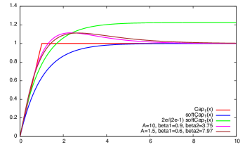
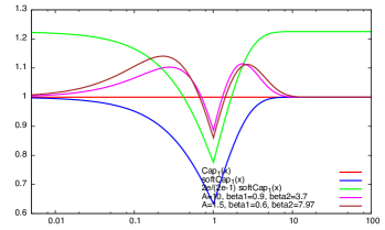
Figure 3. Left: $\textsf{cap}_{1}(w)$ function and different approximations: With a single $\operatorname{\mathcal{L}^{c}}$ point measurement we can use the soft capping function $\widetilde{\textsf{cap}}_{1}(w)$ or scaling it $\frac{2e}{2e-1}\widetilde{\textsf{cap}}_{1}(w)$ to minimize the worst-case relative error. We also show two 3 point measurements approximations with different parameters. Right: The corresponding ratio to $\textsf{cap}_{1}$ which shows the relative error of the different approximations.

8. Experiments

We performed experiments aimed at demonstrating the ease of implementing our schemes and explaining the use of the parameters that control the approximation quality. We implemented the element mapping functions in Python. We also use Python implementations of approximate $\operatorname{\textsf{MxDistinct}}$ and $\operatorname{\textsf{Distinct}}$ sketches. We generated synthetic data using a Zipf distribution of keys. We set the values of all elements to $1$. Zipf distributions are parametrized by $\alpha$ that controls the skew: The distribution is more skewed (has more higherer frequency keys) with higher $\alpha$. Typically values in the range $\alpha\in[1,2]$ model real-world distributions. We used $\alpha=\{1.1,1.2,1.5,2.0\}$ in our experiments.

8.1. Point measurements

In this set of experiments we generated data sets with $10^{5}$ elements and performed point measurements, which approximate the statistics $\widetilde{\textsf{cap}}_{T}(W)$. We used $T=\{1,5,20,100,500\}$. We applied element mapping Algorithm 1 with parameter $r\in\{1,10,100\}$ to generate output elements $E$. The output elements were processed by an approximate distinct counter with parameter $k=100$ to obtain an estimate of $\operatorname{\textsf{Distinct}}(E)$. The final estimate (13) is the approximate count divided by $r$. In our evaluation we also computed the exact count $\operatorname{\textsf{Distinct}}(E)$, to obtain the exact point measurement, and also the exact value of the statistics $\widetilde{\textsf{cap}}_{T}(W)$.

Recall that there are two sources of error in the approximate measurement. The first is the error of the measurement $\widehat{\operatorname{\mathcal{L}^{c}}}[W](t)$ ($\operatorname{\textsf{Distinct}}(E)/r$) as an estimate of $\operatorname{\mathcal{L}^{c}}[W](t)$. This error is controlled by the parameter $r$ in the element mapping Algorithm 1. We showed that $r>\epsilon^{-2.5}$ always suffices in the worst-case but generally on larger data set that are not dominated by few keys we have $\operatorname{\mathcal{L}^{c}}[W](t)>\epsilon^{-2}$ and $r=1$ suffices. The second source of error is the approximate counter which returns an approximation $\widehat{\widehat{\operatorname{\mathcal{L}^{c}}}}[W](t)$ of the measurement $\widehat{\operatorname{\mathcal{L}^{c}}}[W](t)$. An approximate counter with $k=\epsilon^{-2}$ has NRMSE $\epsilon$. In the experiments we used a fixed $k=100$ which has $\epsilon=0.1$. We performed 200 repetitions of each experiment and computed the average errors. Results are illustrated in Figure 4: The left plot in the figure shows the average number of distinct output elements generated for different Zipf parameters $\alpha$ and $T$ value for $r=1$. The expectation of $\operatorname{\textsf{Distinct}}(E)$ is equal to $r\widehat{\operatorname{\mathcal{L}^{c}}}[W](1/T)$. The middle plot shows the normalized root mean squared (NRMSE) error of the measurement $\frac{T}{r}\operatorname{\textsf{Distinct}}(E)$ that uses the exact distinct count of output keys. We can see that the error rapidly decreases with the parameter $r$ and that it is very small. The right plot shows the error of the approximate measurement as a function of $r$, obtained by applying an approximate counter to $E$. The additional error component is an error with NRMSE $10\%$ with respect to the measurement, and is independent of the measurement error. We can see that the approximation error dominates the total error which is about $10\%$.

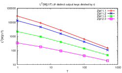
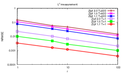
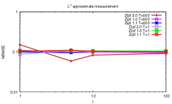
Figure 4. Point measurements experiments on $10^{5}$ elements with Zipf keys (averaged over 200 repetitions). Left: $\operatorname{\mathcal{L}^{c}}[W](1/T)$, Middle: NRMSE of exact measurement $\widehat{\operatorname{\mathcal{L}^{c}}}[W](1/T)$. Right: NRMSE of approximate measurement $\widehat{\widehat{\operatorname{\mathcal{L}^{c}}}}[W](1/T)$.

8.2. Combination measurements

In this set of experiments we estimate the statistics $f(W)$ for $f(w)=\sqrt{w}$ using approximate combinations measurements. We used the element mapping Algorithm 2 with $\tau=0$. Note that the estimates we get are unbiased but the NRMSE error can be larger due to the contributions of the $t$ regime with a very small number of output keys. Figure 5 shows the NRMSE of the measurement $\frac{1}{r}\operatorname{\textsf{MxDistinct}}(E)$ for different values of $r$. The application of an approximate $\operatorname{\textsf{MxDistinct}}$ counter of size $\epsilon^{-2}$ introduces NRMSE of at most $\epsilon$ to this measurement.

Figure 5. Combination measurement NRMSE for $f(w)=\sqrt{w}$ as a function of $r$ on $10^{5}$ elements with Zipf distributed keys, averaged over 200 repetitions.

9. Conclusion

We presented a novel elegant framework for composable sketching of concave sublinear statistics. We obtain state-of-the-art asymptotic bounds on sketch size together with highly efficient practical solution.

We leave open the intriguing question of fully understanding the limits of our approach and in particular, understand if the scope of sample-based sketching is limited to (sub)linear statistics (we suspect it does). Another question is to precisely quantify the approximation tradeoff for $\textsf{cap}_{1}$ (and hence for any $\overline{\textsf{cap}}$ function)

Appendix A Efficient element processing for point measurements

Ideally, we would want to determine the selected indices using computation proportional to $O(r(1-\exp(-t\text{\em{e.value}}))$, which is the expected number of output keys returned. There are many ways to do so and retain the confidence bounds. We recommend a way that uses varopt dependent sampling [3, 18, 8, 10]. This shows that, in principle, we can always obtain very tight concentration for $\widehat{\operatorname{\mathcal{L}^{c}}}[W](t)$ as an approximation of $\operatorname{\mathcal{L}^{c}}[W](t)$ (using large enough $r$).

Pseudocode for the inner loop of the efficient element processing is provided as Algorithm 4. The inner loop selects the samples from $[1,r]$, each in probability $p$, in time proportional to the number of selected samples. The range $[1,r]$ is logically partitioned to $\lceil rp\rceil$ consecutive ranges of size $\lfloor 1/p\rfloor$, where $p=1-\exp(-t\text{\em{e.value}})$ (the last range may be smaller). The probability associated with each range is its size times $p$, which is $p\lfloor 1/p\rfloor\leq 1$. We then varopt sample the $O(pr)$ ranges according to these probabilities (e.g., using $\lceil rp\rceil$ pair aggregations [8]). Finally, for each range that is included in the sample, we uniformly return one of the numbers in the range.

The improved scheme select a varopt sample of the set $[r]$ such that each $i\in[r]$ is included with probability $1-\exp(-t\text{\em{e.value}})$. Since the joint inclusion/exclusion probabilities have the varopt property, the concentration bounds (Lemma 3.2) hold. Moreover, generally varopt improves quality over Poisson sampling by eliminating the variance in the sample size.

$p\leftarrow 1-\exp(-t\text{\em{e.value}})$ // inclusion probability for each $i\in[r]$ // Compute vector $\boldmath{\pi}$ of sampling probabilities for consecutive partition of $[1,r]$ to subranges of equal size $\lfloor 1/p\rfloor$ and the remainder as the last entry.

$\ell\leftarrow\lceil\frac{pr}{p\lfloor 1/p\rfloor}\rceil$

$rem\leftarrow r\,\text{mod}\,p\lfloor 1/p\rfloor$

if $rem=0$ then // $\ell_{f}$ number of full-size ranges

      $\ell_{f}=\ell$

else

      $\ell_{f}=\ell-1$

Initialize a vector $\boldmath{\pi}$ of size $\ell$ foreach $j\leq\ell_{f}$ do

      $\pi_{j}\leftarrow p\lfloor 1/p\rfloor$

if $rem\not=0$ then

      $\pi_{\ell}\leftarrow prem$

// varopt sample the entries of $\boldmath{\pi}$

$S\leftarrow$ varopt sample $\boldmath{\pi}$

  // $S$ has $\lfloor pr\rfloor$ or $\lceil pr\rceil$ entries equal to $1$ and remaining entries are $0$.

foreach $h=1,\ldots,\ell_{f}$ do

       if $S_{h}=1$ then

            $j\sim U[1,\lfloor 1/p\rfloor]$

              // uniformly at random

            

             $i\leftarrow(h-1)\lfloor 1/p\rfloor+j$

             $\textnormal{{OutKeys}}.append(H_{i}(\text{\em{e.key}}))$

      

if $rem\not=0$ and $S_{\ell}=1$ then

      $i\sim U[r-rem+1,r]$

        // uniform at random

      

       $\textnormal{{OutKeys}}.append(H_{i}(\text{\em{e.key}}))$

Algorithm 4 Element processing inner loop with varopt sampling (for $\widehat{\operatorname{\mathcal{L}^{c}}}$ measurements)

We point out a choice of $r$, for uniform element values ($\text{\em{e.value}}=1$ for all elements), which seamlessly guarantees small element processing and tight confidence bounds also when $t$ is very small:

Corollary A.1.

. With uniform elements and $r=c\epsilon^{-2}/t$, we have $O(c\epsilon^{-2})$ element processing and probability of relative error that exceeds $\epsilon$ that is bounded by $2\exp(-c/5)$.

Proof.

The element processing is proportional to the number of outkeys computed and is $\frac{r}{t}(1-\exp(-t))\leq c\epsilon^{-2}$. For the concentration bound we note that $w_{x}\geq 1$ for all active keys, from (15), $\operatorname{\mathcal{L}^{c}}[W](t)\geq(1-1/e)\min\{1,t\}$. ∎

Appendix B Inverse $\operatorname{\mathcal{L}^{c}}$ transform derivations

In this section we derive the expressions for the inverse $\operatorname{\mathcal{L}^{c}}$ transform in Table 1. Our main tool is the following Lemma which expresses the inverse $\operatorname{\mathcal{L}^{c}}$ transform of $f$ in terms of the inverse Laplace transform of the derivative of $f(w)$:

Lemma B.1.

$$(\operatorname{\mathcal{L}^{c}})^{-1}[f(w)](t)=\frac{1}{t}\operatorname{\mathcal{L}}^{-1}[\frac{\partial f(w)}{\partial w}](t)\ ,$$

where $\operatorname{\mathcal{L}}$ is the Laplace transform.

Proof.

We look for a solution $a(t)$ of

$$f(w)=\int_{0}^{\infty}a(t)(1-e^{-wt})dt\ .$$

Differentiating both sides by $w$ we obtain

$$\frac{\partial f(w)}{\partial w}=\int_{0}^{\infty}ta(t)e^{-wt}dt=\operatorname{\mathcal{L}}[a(t)t](w)\ .$$

∎

Lemma B.2.

For all $T>0$,

$$\operatorname{\mathcal{L}^{c}}^{-1}[\widetilde{\textsf{cap}}_{T}(w)](t)=T\delta_{1/T}(t)\ ,$$

where $\delta_{1/T}$ is the Dirac Delta function at $1/T$. For all $p\in(0,1)$,

$$\operatorname{\mathcal{L}^{c}}^{-1}[w^{p}](t)=\frac{p}{\Gamma(1-p)}t^{-(1+p)}\,$$

where $\Gamma$ is the Gamma function.

$$\operatorname{\mathcal{L}^{c}}^{-1}[\ln(1+w)](t)=\frac{e^{-t}}{t}\ .$$

Proof.

The claim for the inverse transform of $f(w)=\widetilde{\textsf{cap}}_{T}(w)$ follows directly from (2). For $f(w)=w^{p}$, we apply Lemma B.1 using $\frac{\partial w^{p}}{\partial w}=pw^{p-1}$. We take the inverse Laplace transform to obtain

$$a(t) = \frac{p}{t}\operatorname{\mathcal{L}}^{-1}[w^{p-1}](t)$$

$$= \frac{p}{t}\frac{t^{-p}}{\Gamma(1-p)}$$

$$= \frac{p}{\Gamma(1-p)}t^{-(1+p)}\ .$$

We now consider $f(w)=\ln(1+w)$ and apply Lemma B.1 substituting the derivative $\frac{\partial f(w)}{\partial w}=\frac{1}{1+w}$ and $\operatorname{\mathcal{L}}^{-1}[1/(w+1)]=e^{-t}$. We obtain

$$a(t)=\frac{1}{t}\operatorname{\mathcal{L}}^{-1}[1/(w+1)](t)=\frac{e^{-t}}{t}\ .$$

∎

Appendix C Double-logarithmic size max-distinct sketches

We outline here basic representation tricks that yield max-distinct sketches of size $O(\log\log n+\epsilon^{-2}\log\epsilon^{-1})$ (assuming $1\leq m_{x}=O(\text{poly}(n))$.) Our sketch contains $k$ registers, where each register corresponds to a balanced “bucket” of output keys. For balance, we can place all keys in all buckets (with different hash function per bucket) or (see Section D) apply stochastic averaging and partition the output elements to buckets according to a partition of $[r]$. For an element $e$ with key that falls in the bucket, we compute $-\ln u_{\text{\em{e.key}}}/\text{\em{e.value}}$ and if smaller than the current register, replace its value. The distribution of the minimum in the bucket is exponential with parameter equals to the sum of $m_{x}$ over keys in the bucket (see e.g. [4]). As in Hyperloglog, we only store exponents with base $b=1+\delta$ (for some appropriate small fixed $\delta$) We apply consistent (per key/bucket) randomized rounding to an integral power of $(1+\delta)$ and store only the negated exponent $y_{i}$ for bucket $i$. The exponent can be stored in $O(\log\log n)$ bits. For different buckets, we can store one exponent and offsets of expected size $O(1)$ per bucket. To obtain the approximate statistics from the sketch we use the estimator

$$\widehat{\operatorname{\textsf{MxDistinct}}(E)}=(k-1)/\sum_{i=1}^{k}b^{-y_{i}}\$$

for the total weight of keys over buckets (when stochastic averaging is not used we need to divide by $k$.)

C.1. Sidelined output elements

We discuss here compact representation of the $\ell=3\epsilon^{-2}$ “sidelined” output keys and their $y$ values $(x_{i},y_{i})$. Roughly, it suffices to store $O(\log\epsilon)$ per sidelined key (and one exponent): An $O(\log\ell)$ representation of a hash of the key that will allow us to tell it apart (with good probability) from new elements with $y$ value in the sidelined range. An offset rounded representation of the $y$ value (so that $\int_{y}^{\infty}a(t)dt$ is approximated within $\epsilon$), and a $\log\epsilon$ representation of the distinct counter bucket and of the random hash $u_{e}$, so that the modification to the approximate counter can be performed when $(x_{i},v_{i})$ leaves the sidelined set.

Appendix D Practical optimization for point measurements

An optimization that applies with approximate distinct counters (including Hyperloglog) that use stochastic averaging is to partition equally the $r$ “output” buckets to the $k$ counter buckets. Then pipe corresponding outkeys to each bucket. In more detail, stochastic averaging counters hash each key to one of $k$ buckets, where each bucket maintains an order statistics (maximum or minimum) of another hash applied to the keys that fall in that bucket. This design can be integrated with our element processing parameter $r$. We direct the $r$ indices of outkeys produced for same element to corresponding buckets in the counter, replacing the hash-based assignment to buckets.

Appendix E All-threshold sketches

At a high level, sample-based distinct count sketches can be extended to all-threshold sketches by considering the distinct sketch of $\textnormal{{OutKeys}}_{t}$ as a function of $t$. It turns out (analysis of all-distance sketches) that the number of points $t$ where the sketch changes as we sweep $t$ is in expectation $\epsilon^{-2}\ln(rn)$. In more detail, the Hyperloglog sketch consists of $k=\epsilon^{-2}$ registers that can only increase as keys are processed. Each register has in expectation $\ln(rn)$ change points as we sweep $t$.

The storage overhead factor of all-threshold sketching is the number of change points of each register ($\ln n$) multiplied by the representation of each $t$ value where the change occurred. We now note that since $\operatorname{\mathcal{L}^{c}}[W](t)$ is smooth and Lipschitz, a small number of $\log(1/\epsilon)$ significant bits and the exponent suffices. Since the change points for each register are an increasing sequence, generally from a polynomial range, it suffices to store changes to the exponent.

With an enhanced sketch, since it records all counts as we sweep $t$, we can apply the HIP estimator [5] to the sketch (with respect to the swept parameter $t$) to obtain full-range estimates for all $t$.

Appendix F Bin Transform

A related discrete transform is the Bin transform $\operatorname{\mathcal{B}}[W](\ell)$ for an integer parameter $\ell>0$ is defined as

$$\operatorname{\mathcal{B}}[W](\ell)\equiv\int_{0}^{\infty}W(w)\ell(1-(1-1/\ell)^{w})dw\ .$$

We present a mapping scheme of elements to outkeys that for parameters $\ell,r$ has expected distinct count equal to the Bin trasform of the frequencies. The mapping applies for data sets of elements with uniform values $\text{\em{e.value}}=1$. We use $r$ sets of $\ell$ independent hash functions $H^{(j)}_{i}$ for $i\in[\ell]$ and $j\in[r]$. The hash functions are applied to element keys and produces output keys. We assume that $H^{(j)}_{i}(x)$ are unique for all $x,i,j$. When processing an element $e$, we draw for each $j\in[r]$, a value $i\sim U[\ell]$ uniformly at random. We generate the output key $H^{(j)}_{i}(\text{\em{e.key}})$. Note that $r$ output keys are generated for each element. Our measurement $\widehat{\operatorname{\mathcal{B}}}[W](\ell)$ is the number of distinct outkeys divided by $r$.

The expected contribution of a key $x$ with weight $w_{x}$ to the measurement (the expected number of distinct outkeys produced for elements with that key divided by $r$) is $\ell(1-(1-1/\ell)^{w})$ which is close to $\operatorname{\mathcal{L}^{c}}$measurements. We focus more on the continuous $\operatorname{\mathcal{L}^{c}}$ transform, however, as it is nicer to work with. A variation of the Bin transform was used in [7] for weighted sampling of keys and it was also proposed to use them for counting (computing statistics over the full data).

Appendix G Extension: Time-decaying aggregation

We presented simple “reductions” from the approximation of (sub)linear growth statistics to distinct or max-distinct counting and sum. We observe that our reductions can also be combined with time-decaying aggregation [14] (e.g., sliding window models), with essentially out-of-the-box use of respective structures for distinct counting and sum. For our enhanced (max-distinct, all-threshold) counters we can obtain time-decaying aggregations for all decay functions by essentially “distance sketching” the time domain (see [5]).

Appendix H Extension: Weighted keys

A useful extension is to approximate aggregations of the form

(55) $$\sum_{x}f(w_{x})v_{x}\ ,$$

where $v_{x}>0$ are intrinsic weight associated with key $x$. With the distribution interpretation, we have $W(w)$ as the weighted sum

$$W(w)=\sum_{x\mid w_{x}=w}v_{x}$$

of all keys with frequency $w_{x}=w$. Our presentation focused on $v_{x}=1$ for all keys. We outline how our algorithms can be extended to handle general $v_{x}$ weights. The assumption here is that $v_{x}$ is available to us when an element with key $x$ is processed.

One application is computing a loss function or its gradient when computing embeddings. The data elements have entity and context pairs $(i,j)$. Each entity $i$ has a current embedding vector $\boldmath{v}_{i}$ and similarly, contexts $j$ have embeddings $\tilde{\boldmath{v}}_{j}$. The pairs are our keys and their values are a function of the inner produce $\boldmath{v}_{i}\cdot\tilde{\boldmath{v}}_{j}$. The weight $w_{x}$ of a key $x=(i,j)$ is the number of occurrences of the key in the data. We would like to estimate (55) efficiently.

When $f$ is a soft capping function, this can be done with a single modified point measurement. For $f\in\overline{\widetilde{\textsf{cap}}}$, we need a modified combination measurement.

The modification for point measurements (Element processing Algorithm 1) produces output elements $(H_{i}(x),v_{x})$ instead of respective output keys. The measurement we seek is then a a weighted distinct statistics of the output elements, which returns the sum $\sum_{y}v_{y}$ over distinct output element keys (divided by $r$). The measurement is approximated using an approximate weighted distinct counter instead of a plain distinct counter.

Weighted distinct statistics are a special case of max-distinct statistics, where elements with a certain key always have the same value. Therefore, they can be approximated using approximate max-distinct counters (see Section 5.2).

The modification of Algorithm 2 needed to obtain a combination measurements of (55) replaces the value $y$ of the output elements generated for an element with key $x$ by the product $v_{x}y$. The elements are processed as before by an approximate max-distinct counter. The quality and structure size tradeoffs remain the same.

References

• [1] N.Β Alon, Y.Β Matias, and M.Β Szegedy. The space complexity of approximating the frequency moments. J. Comput. System Sci., 58:137–147, 1999.
• [2] V.Β Braverman and R.Β Ostrovsky. Zero-one frequency laws. In STOC. ACM, 2010.
• [3] M.Β T. Chao. A general purpose unequal probability sampling plan. Biometrika, 69(3):653–656, 1982.
• [4] E.Β Cohen. Size-estimation framework with applications to transitive closure and reachability. J. Comput. System Sci., 55:441–453, 1997.
• [5] E.Β Cohen. All-distances sketches, revisited: HIP estimators for massive graphs analysis. TKDE, 2015.
• [6] E.Β Cohen. Multi-objective weighted sampling. In HotWeb. IEEE, 2015. full version: http://arxiv.org/abs/1509.07445.
• [7] E.Β Cohen. Stream sampling for frequency cap statistics. In KDD. ACM, 2015. full version: http://arxiv.org/abs/1502.05955.
• [8] E.Β Cohen, G.Β Cormode, and N.Β Duffield. Structure-aware sampling: Flexible and accurate summarization. Proceedings of the VLDB Endowment, 2011.
• [9] E.Β Cohen, N.Β Duffield, H.Β Kaplan, C.Β Lund, and M.Β Thorup. Algorithms and estimators for accurate summarization of unaggregated data streams. J. Comput. System Sci., 80, 2014.
• [10] E.Β Cohen, N.Β Duffield, C.Β Lund, M.Β Thorup, and H.Β Kaplan. Efficient stream sampling for variance-optimal estimation of subset sums. SIAM J. Comput., 40(5), 2011.
• [11] E.Β Cohen and H.Β Kaplan. Summarizing data using bottom-k sketches. In ACM PODC, 2007.
• [12] E.Β Cohen and H.Β Kaplan. Tighter estimation using bottom-k sketches. In Proceedings of the 34th VLDB Conference, 2008.
• [13] E.Β Cohen, H.Β Kaplan, and S.Β Sen. Coordinated weighted sampling for estimating aggregates over multiple weight assignments. VLDB, 2(1–2), 2009. full: http://arxiv.org/abs/0906.4560.
• [14] E.Β Cohen and M.Β Strauss. Maintaining time-decaying stream aggregates. J. Algorithms, 59:19–36, 2006.
• [15] C.Β Estan and G.Β Varghese. New directions in traffic measurement and accounting. In SIGCOMM. ACM, 2002.
• [16] P.Β Flajolet, E.Β Fusy, O.Β Gandouet, and F.Β Meunier. Hyperloglog: The analysis of a near-optimal cardinality estimation algorithm. In Analysis of Algorithms (AofA). DMTCS, 2007.
• [17] P.Β Flajolet and G.Β N. Martin. Probabilistic counting algorithms for data base applications. J. Comput. System Sci., 31:182–209, 1985.
• [18] R.Β Gandhi, S.Β Khuller, S.Β Parthasarathy, and A.Β Srinivasan. Dependent rounding and its applications to approximation algorithms. J. Assoc. Comput. Mach., 53(3):324–360, 2006.
• [19] P.Β Gibbons and Y.Β Matias. New sampling-based summary statistics for improving approximate query answers. In SIGMOD. ACM, 1998.
• [20] G.Β H. Golub and V.Β Pereyra. The differentiation of pseudoinverses and nonlinear least squares problems whose variables separate. SIAM Journal on Numerical Analysis, 10:413–432, 1973.
• [21] Google. Frequency capping: AdWords help, December 2014. https://support.google.com/adwords/answer/117579.
• [22] S.Β Heule, M.Β Nunkesser, and A.Β Hall. HyperLogLog in practice: Algorithmic engineering of a state of the art cardinality estimation algorithm. In EDBT, 2013.
• [23] P.Β Indyk. Stable distributions, pseudorandom generators, embeddings and data stream computation. In Proc. 41st IEEE Annual Symposium on Foundations of Computer Science, pages 189–197. IEEE, 2001.
• [24] W.Β Johnson and J.Β Lindenstrauss. Extensions of Lipschitz mappings into a Hilbert space. Contemporary Math., 26, 1984.
• [25] D.Β M. Kane, J.Β Nelson, and D.Β P. Woodruff. An optimal algorithm for the distinct elements problem. In PODS, 2010.
• [26] D.Β E. Knuth. The Art of Computer Programming, Vol 2, Seminumerical Algorithms. Addison-Wesley, 1st edition, 1968.
• [27] R.Β Morris. Counting large numbers of events in small registers. Comm. ACM, 21, 1977.
• [28] S.Β Nandanwar and N.Β N. Murty. Structural neighborhood based classification of nodes in a network. In KDD. ACM, 2016.
• [29] D.Β P. O’Leary and B.Β W. Rust. Variable projection for nonlinear least squares problems. Computational Optimization and Applications, 54(3):579–593, 2013.
• [30] M.Β Osborne. Facebook Reach and Frequency Buying, October 2014. http://citizennet.com/blog/2014/10/01/facebook-reach-and-frequency-buying/.
• [31] J.Β Pennington, R.Β Socher, and C.Β D. Manning. Glove: Global vectors for word representation. In EMNLP, 2014.
• [32] B.Β RosΓ©n. Asymptotic theory for successive sampling with varying probabilities without replacement, I. The Annals of Mathematical Statistics, 43(2):373–397, 1972.
• [33] B.Β RosΓ©n. Asymptotic theory for order sampling. J. Statistical Planning and Inference, 62(2):135–158, 1997.
• [34] G.Β Salton and C.Β Buckley. Term-weighting approaches in automatic text retrieval. Information Processing & Management, 24(5):513 – 523, 1988.
• [35] J.S. Vitter. Random sampling with a reservoir. ACM Trans. Math. Softw., 11(1):37–57, 1985.