Transient temperature and mixing times of quantum walks on cycles

Abstract

The definition of entanglement temperature for the quantum walk on the line is extended to $N$-cycles, which are more amenable to a physical implementation. We show that, for these systems, there is a linear connection between the thermalization time and the mixing time, and also that these characteristic times become insensitive to the system size when $N$ is larger than a few units.

I Introduction

The concept of quantum walk (QW) is a natural generalization of classical random walks and can be considered a subarea of quantum computation and quantum information Kempe:2003a ; Venegas-Andraca:2008 ; Portugal:Book . The possibility of developing fast quantum algorithms based on QWs has attracted the attention of researchers from different fields and the first successes were provided in Refs. Shenvi:2003 ; Ambainis:2005 . Experimental implementations of QWs have been proposed using many kind of physical setups Manouchehri2014 . Actual implementations were reported through experiments on optical Schreiber2010 and atomic systems Karski2009 ; Zahringer2010 . A new proposal of implementation of QWs on cycles using optomechanical systems is described in Ref. MPO15 .

One of the most striking properties of QWs on lattices is their ability to spread over the lattice linearly in time, as characterized by the standard deviation $\sigma(t)\sim t$, while its classical analog spreads out as the square root of time $\sigma(t)\sim t^{1/2}$ ABNVW01 ; MBSS02 . This characteristic is not preserved in fractal-like structures, as is discussed in Refs. BFP14 ; BFP15 .

QWs also have different mixing properties compared to classical random walks. The mixing time measures the time it takes for the average probability distribution to approach the limiting distribution. The mixing time on $N$-cycles is $O(N\ln N)$, giving a nearly quadratic speedup over the classical walk, and it is the best possible, since the diameter of the graph is a lower bound for the mixing time Aharonov:2000 . Similar results were reported for the hypercube in Ref. MPAD08 .

The notion of temperature of QWs is discussed in Refs. Rom10 ; Rom12 ; RDPM14 ; RS14 by analyzing the entanglement between the coin and the spatial subspaces of the composite Hilbert space of a coined QW on the line. Considering the coin as the main system and tracing out the spatial degrees of freedom, the coin reduced density matrix evolves stochastically and has a limiting configuration as time goes to infinity. Considering the quantum canonical ensemble, an entanglement temperature and other thermodynamical quantities can be defined, which help understand the QW dynamics. In the quantum case, the thermodynamical quantities depend on the initial condition in stark contrast with the classical Markovian behavior.

In all the previous work on QW’s entanglement temperature, the analysis was performed considering the system in thermodynamical equilibrium, which is reached when time goes to infinity. In the present paper we analyze the transient behavior of the entanglement temperature on $N$-cycles. We describe the behavior of the temperature as a function of time and determine how quickly thermal equilibration occurs. Using a threshold $\varepsilon$ analogous to the one used in the definition of the mixing time, we define the thermalization time on $N$-cycles and show that this time depends on $\varepsilon$ as $O(\ln{1}/{\varepsilon})$ for a fixed $N$. On the other hand, for large $N$, the value of the thermalization time is determined only by $\varepsilon$ and does not depend on $N$. We also calculate the thermalization time in the classical case and obtain that it also is independent of the cycle size $N$.

The mixing time of QWs has been extensively analyzed in the literature with the goal of establishing that QWs mix faster than the classical random walk, a result which should be useful for quick sampling Richter:2007 ; Ric07 . In this work we analyze an alternative physical intepretation of the mixing time by establishing a connection between the mixing- and the thermalization times. We show analytically that the thermalization time is proportional to the mixing time, which demonstrates that the mixing time is strongly related with the time that thermodynamic quantities take to reach equilibrium.

The paper is organized as follows. In Sec. II, we discuss the dynamics of QWs on cycles. In Sec. III, we obtain the coin reduced density matrix as a function of time. In Sec. IV, we analyze the asymptotic entanglement temperature on cycles and compare with the results on the infinite line. In Sec. V, we calculate the entanglement temperature as a function of time and connect the mixing time and thermalization time for cycles. In Sec. VI, we discuss the Markovian analogue of the classical thermalization time and compared to its quantum version. Finally, in Sec. VII, we present the main conclusions.

II QW on cycles

The standard QW on the line corresponds to a one-dimensional evolution of a quantum system (the walker) in a direction which depends on an additional degree of freedom, the chirality, with two possible states: “left” $|L\rangle$ or “right” $|R\rangle$. The global Hilbert space of the system is the tensor product $H_{s}\otimes H_{c}$ where $H_{s}$ is the Hilbert space associated to the motion on the line and $H_{c}$ is the chirality Hilbert space. Let us call $T_{-}$ ($T_{+}$) the operators in $H_{s}$ that move the walker one site to the left (right), and $|L\rangle\langle L|$ and $|R\rangle\langle R|$ the chirality projector operators in $H_{c}$. We consider the unitary transformations

$$U(\theta)=\left\{T_{-}\otimes|L\rangle\langle L|+T_{+}\otimes|R\rangle\langle R|\right\}\circ\left\{I\otimes K(\theta)\right\},$$ (1)

where $K(\theta)=\sigma_{z}e^{-i\theta\sigma_{y}}$, $I$ is the identity operator in $H_{s}$, and $\sigma_{y}$ and $\sigma_{z}$ are Pauli matrices acting in $H_{c}$. The unitary operator $U(\theta)$ evolves the state in one time step as $|\Psi(t+1)\rangle=U(\theta)|\Psi(t)\rangle$. The wave vector can be expressed as the spinor

$$|\Psi(t)\rangle=\sum\limits_{k=-\infty}^{\infty}\left[\begin{array}[]{c}a_{k}(t)\\ b_{k}(t)\end{array}\right]|k\rangle,$$ (2)

where the upper (lower) component is associated to the left (right) chirality. The unitary evolution implied by Eq. (1) can be written as the map

$$a_{k}(t+1) =a_{k+1}(t)\,\cos\theta\,+b_{k+1}(t)\,\sin\theta,$$

$$b_{k}(t+1) =a_{k-1}(t)\,\sin\theta\,-b_{k-1}(t)\,\cos\theta,$$ (3)

where $\theta\in\left[0,\pi/2\right]$ is a parameter defining the bias of the coin toss ($\theta=\frac{\pi}{4}$ for an unbiased or Hadamard coin). Then, the cyclic map is achieved by postulating an appropriate periodicity. In one-dimension, the lattice is bent into a ring so that its last site is the nearest neighbor to its first site. If the lattice extends from the site $0$ to the site $N-1$, then we obtain the evolution equations for the cycle by taking subindices modulo $N$. The evolution of Hadamard QWs on cycles was analyzed in Ref. BGKLW03 with the goal of obtaining explicit formulas for the limiting probability distribution. We depart from the approach of this paper because we are interested to analyze the limiting distribution of the reduced coined space. We leave for Appendix A the derivation of coefficients $a_{k}(t)$ and $b_{k}(t)$, and simply quote the result,

$$a_{k}(t) =\sum\limits_{l=0}^{N-1}\upsilon_{kl}c_{l}^{L}(t),$$

$$b_{k}(t) =\sum\limits_{l=0}^{N-1}\upsilon_{kl}c_{l}^{R}(t),$$ (4)

where $\upsilon_{kl}=\frac{1}{\sqrt{N}}\exp\left(\frac{2\pi ikl}{N}\right)$ and the $c_{l}^{L,R}(t)$ are determined from the initial conditions for $a_{k}(0)$ and $b_{k}(0)$.

III Average reduced density operator as a function of time

The unitary evolution of the QW generates entanglement between the coin and position degrees of freedom. This entanglement can be quantified by the associated von Neumann entropy for the reduced density operator CLXGKK05 that defines the entropy of entanglement

$$S(t)=-\mathrm{tr}(\rho_{c}(t)\ln\rho_{c}(t)),$$ (5)

where

$$\rho_{c}(t)=\mathrm{tr}(|\Psi(t)\rangle\langle\Psi(t)|),$$ (6)

and the partial trace is taken over the positions. Using Eq. (2) and its normalization properties, we obtain the reduced density operator

$$\rho_{c}(t)=\left(\begin{array}[]{cc}P_{L}(t)&Q(t)\\ Q(t)^{\ast}&P_{R}(t)\end{array}\right),$$ (7)

where the global left and right chirality probabilities are defined as

$$P_{L}(t) \equiv\sum_{k=0}^{N-1}\left|a_{k}(t)\right|^{2},\,$$ (8)

$$P_{R}(t) \equiv\sum_{k=0}^{N-1}\left|b_{k}(t)\right|^{2},$$ (9)

with $P_{R}(t)+P_{L}(t)=1$ and the interference term is defined as

$$Q(t)\equiv\sum_{k=0}^{N-1}a_{k}(t)b_{k}^{\ast}(t).$$ (10)

Due to the unitarity of evolution of closed quantum systems, the probability distributions $P_{L}(t)$ and $P_{R}(t)$ do not converge when time goes to infinity. However, we can use a natural notion of convergence in the quantum case, if we define the average of the probability distributions over time. As we shall see, with this definition the results for a large cycle approach those for the quantum walk on the line. For instance, the average of ${P}_{L}(t)$ is

$$\bar{P}_{L}(t)=\frac{1}{t}\sum_{t^{\prime}=0}^{t-1}P_{L}(t^{\prime}).$$ (11)

$\bar{P}_{R}(t)$ and $\bar{Q}(t)$ are obtained in the same manner. These definitions correspond to the natural concept of sampling from the system, since if one measures the system at a random time chosen from the interval $\left[0,t\right]$, the resulting distribution is exactly the average probability distribution.

The average reduced density operator is

$$\bar{\rho}_{c}(t)\equiv\left(\begin{array}[]{cc}\bar{P}_{L}(t)&\bar{Q}(t)\\ \bar{Q}^{\ast}(t)&\bar{P}_{R}(t)\end{array}\right)$$ (12)

and its limit when $t\rightarrow\infty$ is

$$\bar{\rho}_{c}(\infty)=\left(\begin{array}[]{cc}{\Pi}_{L}&{Q_{0}}\\ {Q_{0}}^{\ast}&{\Pi}_{R}\end{array}\right),$$ (13)

where ${\Pi}_{L}$, ${\Pi}_{R}$, and ${Q}_{0}$ are the limiting probability distribution, which are obtained from $\bar{P}_{L}(t)$, $\bar{P}_{R}(t)$, and $\bar{Q}(t)$, respectively, after taking the limit $t\rightarrow\infty$, and are given in AppendixB. Ref. Aharonov:2000 addressed a similar calculation by tracing out the coin space.

It is interesting to point out that Eq. (12) can be expressed as

$$\bar{\rho}_{c}(t)=\bar{\rho}_{c}(\infty)+\frac{2}{t}\left(\begin{array}[]{cc}\xi(t)&\varsigma(t)\\ \varsigma^{\ast}(t)&-\xi(t)\end{array}\right),$$ (14)

where $\xi(t)$ and $\varsigma(t)$ are functions of $t$, whose expressions are obtained in Appendix B. Eq. (14) shows that the convergence of $\bar{\rho}_{c}(t)$ to its asymptotic value goes essentially as $1/t$.

IV Asymptotic entanglement temperature

The eigenvalues of $\bar{\rho}_{c}(\infty)$ given by Eq. (13) are

$$\bar{\Lambda}^{\pm}=\frac{1}{2}\left[1\pm\sqrt{1-4\left(\Pi_{L}\,\Pi_{R}-\left|Q_{0}\right|^{2}\right)}\right],$$ (15)

and can be expressed in the following form

$$\bar{\Lambda}^{\pm}=\frac{1}{2}\pm\sqrt{\chi}.$$ (16)

Ref. Rom12 proposed a correspondence between $\bar{\Lambda}^{\pm}$ and the probabilities of being in the ground and excited states of a two-state system. Using the canonical ensemble and a two-state Hamiltonian with energy levels $\pm E_{0}$, we have

$$\bar{\Lambda}^{\pm}\,=\,\frac{e^{\pm\beta E_{0}}}{e^{\beta E_{0}}+e^{-\beta E_{0}}},$$ (17)

where $\beta=1/T$. Solving for $T$, we obtain the expression for the asymptotic entanglement temperature:

$$T=2E_{0}/\ln\left(\frac{1+2\sqrt{\chi}}{1-2\sqrt{\chi}}\right).$$ (18)

Once the value of $\chi$ is known, the temperature is completely determined.

In order to analyze details about this asymptotic temperature on $N$-cycles and to show the differences with respect to the entanglement temperature on the infinite line (analyzed in Ref. Rom12 ), we consider a QW on $N$-cycles with a localized initial condition, that is, the initial position of the walker is assumed to be at the origin with arbitrary chirality. Then

$$\left[\begin{array}[]{c}a_{k}(0)\\ b_{k}(0)\end{array}\right]=\delta_{k0}\left[\begin{array}[]{c}\cos{\frac{\gamma}{2}}\\ e^{i\varphi}\text{ }\sin{\frac{\gamma}{2}}\end{array}\right],$$ (19)

where $\gamma\in\left[0,\pi\right]$ and $\varphi\in\left[0,2\pi\right]$ define a point on the unit three-dimensional Bloch sphere (see Eq. (2)).

Using the results of Appendices A and B and after some algebra, we obtain the following expressions for the the limiting probability distributions:

$${\Pi}_{L} =1-{\Pi}_{R},$$ (20)

$${\Pi}_{R} =\left(\frac{1}{2}-\frac{1}{2}\cos^{2}\theta\cos\gamma-\frac{1}{4}\sin\gamma\sin{2\theta}\cos\varphi\right)f(N,\theta)$$

$$+\left(\frac{1}{4}\sin\gamma\sin{2\theta}\cos\varphi-\cos^{2}\theta\sin^{2}\frac{\gamma}{2}\right)g(N,\theta),$$ (21)

$${Q_{0}} =\frac{1}{4}\left(e^{-i\varphi}\sin\gamma\sin^{2}\theta+\frac{1}{2}\cos\gamma\sin 2\theta\right)f(N,\theta)$$

$$+\frac{1}{4}\left(e^{i\varphi}\sin\gamma\sin^{2}\theta+\frac{1}{2}\cos\gamma\sin 2\theta\right)h(N,\theta),\,$$ (22)

where

$$f(N,\theta) =\frac{1}{N}\sum_{k=0}^{N-1}{\frac{1}{1-\cos^{2}\theta\sin^{2}{\frac{2\pi k}{N}}}},$$ (23)

$$g(N,\theta) =\frac{1}{\cos^{2}\theta}(f(N,\theta)-1),$$ (24)

$$h(N,\theta) =\frac{2}{\cos^{2}\theta}+\left(1-\frac{2}{\cos^{2}\theta}\right)f(N,\theta).$$ (25)

Fixing the bias of the coin toss $\theta=\pi/4$, it is possible to show that

$$f(N,\pi/4)=\left\{\begin{array}[]{c}\frac{\left(1+\sqrt{2}\right)^{N}+\left(1-\sqrt{2}\right)^{N}}{\left(1+\sqrt{2}\right)^{N}-\left(1-\sqrt{2}\right)^{N}}\sqrt{2}\\ \frac{\left(1+\sqrt{2}\right)^{N/2}+\left(1-\sqrt{2}\right)^{N/2}}{\left(1+\sqrt{2}\right)^{N/2}-\left(1-\sqrt{2}\right)^{N/2}}\sqrt{2}\end{array}\right.\begin{array}[]{c}\text{for }N\text{ odd},\\ \text{for }N\text{ even}.\end{array}$$

Additionally, using again Eq. (23) and taking $N\rightarrow\infty$, it is straightforward to show that

$$f(N,\theta)\rightarrow\frac{1}{\sin\theta}.$$

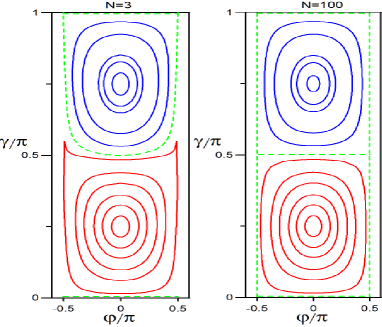
Figure 1: (Color online) Isothermal curves as functions of the initial position, Eq. (19), expressed by the two dimensionless angles $\gamma$ and $\varphi$. The left and right side of the figure correspond for two QWs on the cycle with $N=3$ and $N=100$ respectively. In both sub-figures the bias of the coin is $\theta=\pi/4$. Due to the rotation symmetry in the angle $\varphi$ only two zones are distinguished in each figure: one “cold” and one “hot”. For the “hot” zones (the orange lines on the lower part of the figure) six isotherms are shown, and their temperatures are, starting for the most inner one, $T/T_{0}=6.5,~{}3.2,~{}2.2,~{}1.6,~{}1.3$ and $1.06$. In the case of the “cold” zones (blue lines in the upper part of the figure) five isotherms are shown, and their temperatures are, starting from the outermost one: $T/T_{0}=0.9,~{}0.8,~{}0.7,~{}0.68$ and $0.66$. The dashed green lines correspond to $T/T_{0}=1$.

Using Eqs. (20-22) for a fixed $\theta$, the asymptotic isothermal lines as a function of the initial conditions are determined by the equation

$$\chi= \left[h(N,\theta)-f(N,\theta)\right]^{2}\sin^{2}\varphi\sin^{2}\gamma\sin^{4}\theta/16$$

$$+ \left[h(N,\theta)+f(N,\theta)\right]^{2}\left(\cos\varphi\sin\gamma\sin\theta\right.$$

$$+ \left.{\cos\gamma}\cos\theta\right)^{2}/16.$$ (26)

If we simultaneously make the substitutions $\pi-\gamma\rightarrow\gamma$ and $\varphi+\pi\rightarrow\varphi$, then Eq. (26) is invariant. The angles $\gamma$ and $\varphi$ define the initial chirality on the Bloch sphere, and the mentioned invariance implies that the asymptotic behavior has a symmetry with respect to the origin. This means that any point on the Bloch sphere has the following property

$$\left[X(\varphi+\pi,\pi-\gamma),Y(\varphi+\pi,\pi-\gamma),Z(\varphi+\pi,\pi-\gamma)\right]$$

$$= -\left[X(\varphi,\gamma),Y(\varphi,\gamma),Z(\varphi,\gamma)\right].$$ (27)

Therefore, due to this property, it is sufficient to study the asymptotic isothermal lines as a function of the initial conditions, see Eq. (19), for $\varphi\in\left[-\pi/2,\pi/2\right]$ and $\gamma\in\left[0,\pi\right]$. From Eq. (26), with $\gamma=\pi$, we define

$$\chi_{0}\equiv\left[h(N,\theta)+f(N,\theta)\right]^{2}\frac{\cos^{2}\theta}{16}.$$ (28)

This value $\chi_{0}$ determines, using Eq. (18), the characteristic temperature $T_{0}$. Then the entanglement temperature of the system can be expressed in terms of $T_{0}$.

Fig. 1 shows the level curves (isotherms) for the entanglement temperature as a function of the QW initial position for two QWs on the cycle with $N=3$ (left) and $N=100$ (right). The initial position is defined through the angles $\gamma$ and $\varphi$. Both sides of the figure show two regions, one of them corresponding to temperatures $T>T_{0}$ (the orange lines in the lower regions) and the other to temperatures $T<T_{0}$ (the blue lines in the upper regions). The dashed green straight lines correspond to the temperature $T=T_{0}$ and their initial conditions are $\gamma=\pi$. From this figure it is clear that the dependence of the temperature with the size $N$ of the cycle is very weak. This arises from the fact that the convergence of $f(N,\theta)$ and $h(N,\theta)$, Eqs. (23) and (25), with $N$ is very fast. Additionally, it is important to point out that taking $N\rightarrow\infty$ we re-obtain analytically the asymptotic behavior of the QW on the line reported in Ref. Rom12 . This last result indicates that the extension of the entanglement temperature to finite graphs, as proposed in this work, is consistent.

V Transient Entanglement Temperature

In this section we analyze the thermal transient behavior on $N$-cycles. Using the same correspondence between the eigenvalues of the reduced density operator and the energy levels of a two-state Hamiltonian for any time $t$ (given by Eq. (17) in the asymptotic case), we can define a transient entanglement temperature by using the expression

$$T(t)\,=\,\frac{E_{0}}{\ln{\left(\bar{\Lambda}^{+}(t)/\bar{\Lambda}^{-}(t)\right)}},$$ (29)

where $\bar{\Lambda}^{\pm}(t)$ are the eigenvalues of $\bar{\rho}_{c}(t)$ given by Eq. (12). We assume that $\Lambda^{+}(t)>\Lambda^{-}(t)$.

Fig. 2 presents three curves for the entanglement temperature as a function of time. They are calculated using the original map given by Eq. (3). This figure shows that the temperature quickly approaches a limiting value in $t\sim 100$ time steps.

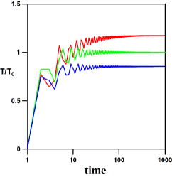
Figure 2: (Color online) Dimensionless entanglement temperatures as a function of time, in log scale, for $N=3$ and $\theta=\pi/4$. Starting from the bottom to the top, the asymptotic temperatures are $T/T_{0}=0.8,1$ and $1.1$. The initial conditions for these curves can be obtained from Fig. 1.

Let us now connect this thermalization process with the convergence of the density distribution. The usual mixing time is defined from the density matrix as

$$\tau_{\varepsilon}(N)\equiv\min\{\widetilde{t}\ |\ \forall t\geq\widetilde{t},\|\bar{\rho}_{c}(t)-\bar{\rho}_{c}(\infty)\|\leq\varepsilon\}$$ (30)

where $\varepsilon$ is an arbitrarily small positive number. For the norm in Eq. (30) we employ the definition

$$\|\bar{\rho}_{c}(t_{1})-\bar{\rho}_{c}(t_{2})\|\equiv\left|\bar{\Lambda}^{+}(t_{1})-\bar{\Lambda}^{+}(t_{2})\right|.$$ (31)

It is straightforward to show that this definition meets the requirements of a properly defined seminorm, it i.e. absolute homogeneity and subaditivity. The elements of the density matrix $\bar{\rho}_{c}(t)$ converge to the corresponding ones of $\bar{\rho}_{c}(\infty)$. Besides, aside from a set of initial conditions of measure zero, $\bar{\Lambda}^{+}(t_{1})=\bar{\Lambda}^{+}(t_{2})\Leftrightarrow t_{1}=t_{2}$. This is a direct consequence of the evolution being over discrete values of the time. Therefore the definition in Eq.(31) can be considered as a true norm for the definition of the mixing time in Eq.(30).

Using Eq. (12) we obtain

$$\bar{\Lambda}^{\pm}(t)=\frac{1}{2}\left[1\pm\sqrt{1-4\left(\bar{P}_{L}(t)\,\bar{P}_{R}(t)-\left|\bar{Q}(t)\right|^{2}\right)}\right],$$ (32)

and from Eq. (29) it is straightforward to show that

$$\tanh\left(\beta(t)E_{0}\right)=\sqrt{1-4\left(\bar{P}_{L}(t)\,\bar{P}_{R}(t)-\left|\bar{Q}(t)\right|^{2}\right)},$$ (33)

where we have defined $\beta(t)=1/T(t)$.

$$\bar{\Lambda}^{+}(t)-\bar{\Lambda}^{+}(\infty)=\frac{1}{2}\left[\tanh\left(\beta(t)E_{0}\right)-\tanh\left(\beta(\infty)E_{0}\right)\right].$$ (34)

Defining $\Delta\beta=\beta(t)-\beta(\infty)$ and using that $\Delta\beta$ goes to zero when $t$ is large we obtain

$$\bar{\Lambda}^{+}(t)-\bar{\Lambda}^{+}(\infty)=\frac{E_{0}}{c}\,\Delta\beta+O(\Delta\beta^{2})$$ (35)

where

$$c=2\cosh^{2}\left(\beta(\infty)E_{0}\right).$$ (36)

If we now define the thermodynamic thermalization time as

$$\tilde{\tau}_{\varepsilon}(N)\equiv\min\{\widetilde{t}\ |\ \forall t\geq\widetilde{t},E_{0}|\beta(t)-\beta(\infty)|\leq\varepsilon\},$$ (37)

we see that the mixing and thermalization times are related through

$$\tau_{\varepsilon}(N)\simeq\tilde{\tau}_{c\varepsilon}(N)$$ (38)

for large $t$, where $\tilde{\tau}_{c\varepsilon}(N)$ is defined by Eq. (37) after replacing $\varepsilon$ by $c\varepsilon$.

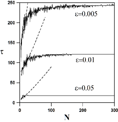
Figure 3: Mixing time as a function of $N$. In all calculations we took $\theta=\pi/4$, $\gamma=\pi/3$ and $\varphi=\pi/6$. A fit of $\tau$ with the function $N\ln N$ for an initial small range of values of $N$ is shown with dashed lines.

The mixing time depends on both $N$ and $\varepsilon$. Fig. 3 depicts the mixing time as a function of $N$ for several values of $\varepsilon$. Notice that $\tau_{\varepsilon}$ does not depend on $N$ for large $N$. However, $\tau_{\varepsilon}$ depends on $N$ for small values of $N$, and when $\varepsilon$ is very small, $\tau_{\varepsilon}$ is independent of $N$ only for large $N$. Additionally, Fig. 3 shows that $\tau_{\varepsilon}=O(1/\varepsilon)$ for $N$ large. This behavior is a direct consequence of Eq. (14), which shows that $\|\bar{\rho}_{c}(t)-\bar{\rho}_{c}(\infty)\|\sim 1/t$. A similar conclusion can be reached by using the Riemann-Lebesgue lemma PBF15 . Using this result we obtain

$$\tau_{\varepsilon}\simeq\tilde{\tau}_{\varepsilon}/c.$$ (39)

Thus, there is a linear connection between the mixing time and the thermalization time, and those quantities do not depend on the system size when $N$ is large for fixed $\varepsilon$. From the expression for $c$ given in Eq.(36), we see that, for small values of the equilibrium entanglement temperature, the mixing time is a small fraction of the thermalization time.

VI Markovian version of the Quantum Walk on the cycle

It is shown in Refs. Rom10 ; Rom12 that $P_{L}$, $P_{R}$ and $Q$ satisfies the following map

$${\left[\begin{array}[]{c}P_{L}(t+1)\\ P_{R}(t+1)\end{array}\right]} ={\left(\begin{array}[]{cc}\cos^{2}\theta&\sin^{2}\theta\\ \sin^{2}\theta&\cos^{2}\theta\end{array}\right)}\left[\begin{array}[]{c}P_{L}(t)\\ P_{R}(t)\end{array}\right]$$ (46)

$$+\mathrm{Re}\left[Q(t)\right]\sin{2}\theta\left[\begin{array}[]{c}1\\ -1\end{array}\right].$$ (49)

This equation is valid for both the QW on the line as on the cycle and from it is clear that $Q(t)$ accounts for the interferences. When $Q(t)$ vanishes the behavior of $[P_{L}(t),P_{R}(t)]$ can be described as a classical Markovian process. Therefore, the classical analogous map for the quantum walk on the cycle (Eq. (49)) is given by the following equations

$${\left[\begin{array}[]{c}P_{mL}(t+1)\\ P_{mR}(t+1)\end{array}\right]} ={\left(\begin{array}[]{cc}\cos^{2}\theta&\sin^{2}\theta\\ \sin^{2}\theta&\cos^{2}\theta\end{array}\right)}\left[\begin{array}[]{c}P_{mL}(t)\\ P_{mR}(t)\end{array}\right],$$ (56)

where the additional subindex $m$ (in $P_{mL}$ and $P_{mR}$) refers to the Markovian character of this distribution. The solution of this map is

$${\left[\begin{array}[]{c}P_{mL}(t)\\ P_{mR}(t)\end{array}\right]}$$ (59)

$$=\frac{1}{2}{\left(\begin{array}[]{cc}1+\cos^{t}(2\theta)&1-\cos^{t}(2\theta)\\ 1-\cos^{t}(2\theta)&1+\cos^{t}(2\theta)\end{array}\right)}\left[\begin{array}[]{c}P_{mL}(0)\\ P_{mR}(0)\end{array}\right],$$ (64)

and its asymptotic behavior is independent of the initial condition

$$\begin{array}[]{c}\lim\text{ }P_{mL}(t)\\ t\rightarrow\infty{}{}{}{}\end{array} =\frac{1}{2},\,$$ (67)

$$\begin{array}[]{c}\lim\text{ }P_{mR}(t)\\ t\rightarrow\infty{}{}{}{}\end{array} =\frac{1}{2}.$$ (70)

The reduced density matrix in this case is

$$\rho_{mc}(t)=\left(\begin{array}[]{cc}P_{mL}(t)&0\\ 0&P_{mR}(t)\end{array}\right).$$ (71)

If we assume equilibrium between the lattice and the chirality, it is possible to define a time-dependent transient temperature for the Markovian process in the same way than in the quantum case, that is

$$P_{mL}(t)\equiv\frac{e^{\beta_{m}E_{0}}}{e^{\beta_{m}E_{0}}+e^{-\beta_{m}E_{0}}},$$ (72)

$$P_{mR}(t)\equiv\frac{e^{-\beta_{m}E_{0}}}{e^{\beta_{m}E_{0}}+e^{-\beta_{m}E_{0}}},$$ (73)

where

$$\beta_{m}(t)=\frac{1}{2E_{0}}\ln\left\{\frac{1+\cos^{t}(2\theta)(P_{mL}(0)-P_{mR}(0))}{1-\cos^{t}(2\theta)(P_{mL}(0)-P_{mR}(0))}\right\}.$$ (74)

The above equation shows that in the asymptotic limit of large $t$ the temperature is infinite, independently of the initial conditions, and the chirality is equally distributed between left and right. Using Eq. (37) we obtain

$$\tilde{\tau}_{\varepsilon}(N)\approx\frac{\ln\varepsilon-\ln|P_{mL}(0)-P_{mR}(0)|}{\ln|\cos(2\theta)|},$$ (75)

for small $\varepsilon$. We note that, differing from the quantum case, $\tilde{\tau}_{\varepsilon}(N)$ does not depend on $N$ even for small $N$, and it is valid for both the line and cycle. Note that, according to Eq. (56), for $\theta=0$ the probabilities $P_{L,R}(t)$ are constant. Thus, in this case, as well as for $\theta=\frac{\pi}{4}$, which corresponds to the usual Hadamard coin, the thermalization time vanishes. For $\theta=\frac{\pi}{2}$ the probabilities $P_{L,R}(t)$ flip-flop without converging, so the system does not thermalize. For other values of $\theta$ the thermalization time scales as $\tilde{\tau}_{\varepsilon}(N)=O\big{(}\ln\frac{1}{\varepsilon}\big{)}$.

VII Conclusions

We have studied the asymptotic regime of QWs on $N$-cycles and we have focused into the asymptotic entanglement between chirality and position degrees of freedom in order to define the entanglement temperature on cycles, generalizing the definition obtained for the line in Ref. Rom12 . A map for the isotherms was analytically built for arbitrary localized initial conditions and found that the entanglement temperature depends strongly on the initial conditions of the system but weakly with the cycle size $N$. We have also verified that when $N\rightarrow\infty$ the thermodynamic behavior of the QW on the line is recovered.

Then we have focused on the transient behavior of the QW on $N$-cycles. We have extended the definition of entanglement temperature for times where the equilibrium thermodynamic between chirality and position was still not achieved. Using this temperature, we have introduced the concept of thermalization time. One of the main results of this work was to show that the thermalization time is proportional to the mixing time, a result which provides a new interpretation of the concept of mixing times of QWs in terms of the time that thermodynamic quantities take to reach the equilibrium. The mixing time in our case is defined as the time it takes for the average global chirality be $\varepsilon$-close to its limiting distribution. We have numerically shown that, fixing $\varepsilon$, the mixing time depends on $N$ only for small values of $N$, and becomes practically independent on the system’s size when $N$ is large. This last fact shows that the entanglement between the coin and position degrees of freedom achieves equilibrium in a much faster way than the density distribution associated to the full wave function. For a given threshold $\varepsilon$, the mixing time is at most half of the thermalization time, and their ratio becomes much smaller for small values of the equilibrium entanglement temperature.

Finally, we have built and studied the chirality distribution for the classical analogous of QWs on $N$-cycles. In this case the chirality distribution has a Markovian behavior and the mixing time does not depend of $N$ even for a small $N$.

Appendix A

In order to uncouple the chirality components in Eqs. (3), we consider two consecutive time steps and rearrange the corresponding evolution equations to obtain

$$a_{k}(t+1)\,-a_{k}(t-1) =\cos\theta\text{ }\left[a_{k+1}(t)\,-a_{k-1}(t)\right],$$

$$b_{k}(t+1)\,-b_{k}(t-1) =\cos\theta\text{ }\left[b_{k+1}(t)\,-b_{k-1}(t)\right],$$ (76)

for $0\leq k\leq N-1$. Note that, after the last transformation, both components of the chirality satisfy the same equation. These equations can be put in matrix form

$$\overrightarrow{A}(t+1)-\overrightarrow{A}(t-1) =M\text{ }\overrightarrow{A}(t),$$

$$\overrightarrow{B}(t+1)-\overrightarrow{B}(t-1) =M\text{ }\overrightarrow{B}(t),$$ (77)

where

$$\overrightarrow{A}(t) =\left[a_{0}(t),...,a_{N-1}(t)\right]^{T},$$

$$\overrightarrow{B}(t) =\left[b_{0}(t),...,b_{N-1}(t)\right]^{T},$$

and $M$ is

$$\cos\theta\left(\begin{array}[]{cccccccc}\ 0&\ \ 1&0&0&...&0&0&-1\\ -1&\ 0&1&0&...&0&0&0\\ \ 0&-1&0&1&...&0&0&0\\ .&.&.&.&...&.&.&.\\ .&.&.&.&...&.&.&.\\ \ 0&\ 0&0&0&...&-1&0&1\\ \ 1&\ 0&0&0&...&\ \ 0&-1&0\end{array}\right).$$ (78)

Then, $M$ is a cyclic square matrix, with dimensionality $N\times N$. Following Ref. BK52 , the characteristic values and vectors of the matrix Eq. (78) are respectively

$$\lambda_{k\text{ }}=2i\cos\theta\sin\left(\frac{2\pi k}{N}\right),$$ (79)

and

$$\upsilon_{kl}=\frac{1}{\sqrt{N}}\exp\left(\frac{2\pi ikl}{N}\right),$$ (80)

where $\upsilon_{kl}$ denotes the $l$th component of the eigenvector associated with the eigenvalue $\lambda_{k}$ and the indices $k$ and $l$ run from $0$ to $N-1$. We now proceed to solve Eqs. (77) in the base where the matrix $M$ is diagonal. To do this, we multiply both sides of Eqs. (77) by the inverse of the matrix $\upsilon_{kl}$ and define the vectors $c_{k}^{L,R}(t)$ as

$${c_{k}^{L}(t)} ={\sum\limits_{l=0}^{N-1}{\upsilon}_{kl}^{\ast}\text{ }a_{l}(t)},$$

$${c_{k}^{R}(t)} ={\sum\limits_{l=0}^{N-1}{\upsilon}_{kl}^{\ast}\text{ }b_{l}(t)},$$ (81)

where ${\upsilon}_{kl}^{\ast}$ is the complex conjugate of ${\upsilon}_{kl}$. Therefore the amplitudes $c_{k}^{L,R}(t)$ satisfy the fundamental equation

$$c_{k}^{L,R}(t+1)-c_{k}^{L,R}(t-1)=\lambda_{k\text{ }}c_{k}^{L,R}(t).$$ (82)

If $c_{k}^{L,R}(0)$ and $c_{k}^{L,R}(1)$ are the amplitudes evaluated into two consecutive initial time steps, then the time dependent solution of Eq. (82) is

$$c_{k}^{L,R}(t)=\alpha_{k}^{L,R}\text{ }e^{i\Omega_{k}t}+\beta_{k}^{L,R}(-1)^{t}e^{-i\Omega_{k}t},$$ (83)

where

$$\sin\Omega_{k}\equiv\cos\theta\sin\left(\frac{2\pi k}{N}\right)=\frac{\lambda_{k\text{ }}}{2i},$$ (84)

$$\alpha_{k}^{L,R}\equiv\frac{c_{k}^{L,R}(1)+c_{k}^{L,R}(0)e^{-i\Omega_{k}}}{2\cos\Omega_{k}},$$ (85)

$$\beta_{k}^{L,R}\equiv\frac{c_{k}^{L,R}(0)e^{i\Omega_{k}}-c_{k}^{L,R}(1)}{2\cos\Omega_{k}}.$$ (86)

Using the orthogonality property

$$\sum\limits_{l=0}^{N-1}\upsilon_{k^{\prime}l}\upsilon_{kl}^{\ast}=\delta_{kk^{\prime}},$$

where $\upsilon_{lk}^{\ast}$ is the transposed conjugate of $\upsilon_{kl}$, we can return to the initial variables by making an inverse transform of Eqs. (81), that is

$$a_{k}(t) =\sum\limits_{l=0}^{N-1}\upsilon_{kl}c_{l}^{L}(t),$$

$$b_{k}(t) =\sum\limits_{l=0}^{N-1}\upsilon_{kl}c_{l}^{R}(t),$$

i.e. Eq.(4). The conditions $c_{k}^{L,R}(0)$ and $c_{k}^{L,R}(1)$ can be obtained using the initial conditions for $a_{k}(0)$ and $b_{k}(0)$ into Eqs. (3) for $t=0$.

Appendix B

The functions $\xi(t)$ and $\varsigma(t)$ used in Eq. (14) are given by:

$$\xi(t) \equiv\sum_{k=0}^{N-1}\mathfrak{R}\left\{\alpha_{k}^{L}\beta_{k}^{L\ast}\mathfrak{F}_{k}(t)\right\},\,$$ (87)

$$\varsigma(t) \equiv\frac{1}{2}\sum_{k=0}^{N-1}\left\{{\alpha_{k}^{L}\beta_{k}^{R\ast}\mathfrak{F}_{k}(t)+\beta_{k}^{L}\alpha_{k}^{R\ast}\mathfrak{F}_{k}^{\ast}(t)}\right\},\,$$ (88)

$$\mathfrak{F}_{k}(t) =\frac{1-e^{i(2\Omega_{k}+\pi)t}}{1+e^{2i\Omega_{k}}}\,,$$ (89)

where $\mathfrak{R}\left\{x\right\}$ is the real part of $x$.

In order to obtain the above result we use the following expressions:

$${\Pi}_{L} =\sum_{k=0}^{N-1}\left\{\left|\alpha_{k}^{L}\right|^{2}+\left|\beta_{k}^{L}\right|^{2}\right\},\,$$ (90)

$${\Pi}_{R} =\sum_{k=0}^{N-1}\left\{\left|\alpha_{k}^{R}\right|^{2}+\left|\beta_{k}^{R}\right|^{2}\right\},\,$$ (91)

$${Q_{0}} =\sum_{k=0}^{N-1}\left\{{\alpha_{k}^{R}}^{\ast}\alpha_{k}^{L}+{\beta_{k}^{R}}^{\ast}\beta_{k}^{L}\right\}.\,$$ (92)

In the last three equations we have introduced the superscript $R$ and $L$ to indicate whether the initial constants, $\alpha_{k}$ and $\beta_{k}$, are related to the initial conditions over $a_{k}$ or $b_{k}$, respectively.

Substituting Eqs. (85) and (86) into Eqs. (90), (91) and (92) we obtain

$${\Pi}_{L} =\sum_{k=0}^{N-1}\frac{\left|c_{k}^{L}(1)\right|^{2}+\left|c_{k}^{L}(0)\right|^{2}}{2\cos^{2}\Omega_{k}}$$

$$+\sum_{k=0}^{N-1}\frac{i\sin\Omega_{k}(c_{k}^{L}(1){c_{k}^{L}}^{\ast}(0)-{c_{k}^{L}}^{\ast}(1)c_{k}^{L}(0))}{2\cos^{2}\Omega_{k}},\,$$ (93)

$${\Pi}_{R} =\sum_{k=0}^{N-1}\frac{\left|c_{k}^{R}(1)\right|^{2}+\left|c_{k}^{R}(0)\right|^{2}}{2\cos^{2}\Omega_{k}}$$

$$+\sum_{k=0}^{N-1}\frac{i\sin\Omega_{k}(c_{k}^{R}(1){c_{k}^{R}}^{\ast}(0)-{c_{k}^{R}}^{\ast}(1)c_{k}^{R}(0))}{2\cos^{2}\Omega_{k}},\,$$ (94)

$${Q_{0}} =\sum_{k=0}^{N-1}\frac{c_{k}^{L}(0){c_{k}^{R}}^{\ast}(0)+c_{k}^{L}(1){c_{k}^{R}}^{\ast}(1)}{2\cos^{2}\Omega_{k}}$$

$$+\sum_{k=0}^{N-1}\frac{i\sin\Omega_{k}(c_{k}^{L}(1){c_{k}^{R}}^{\ast}(0)-c_{k}^{L}(0){c_{k}^{R}}^{\ast}(1))}{2\cos^{2}\Omega_{k}}.\,$$ (95)

References

- (1) J. Kempe. Quantum random walks - an introductory overview. Contemporary Physics, 44(2):307–327, 2003.
- (2) S. E. Venegas-Andraca. Quantum walks for computer scientists. Morgan & Claypool, 2008.
- (3) Renato Portugal. Quantum Walks and Search Algorithms. Springer, New York, 2013.
- (4) N. Shenvi, J. Kempe, and K. B. Whaley. Quantum random-walk search algorithm. Phys. Rev. A, 67:052307, 2003.
- (5) A. Ambainis, J. Kempe, and A. Rivosh. Coins make quantum walks faster. In Proceedings of the 16th ACM-SIAM Symposium on Discrete Algorithms, pages 1099–1108, 2005.
- (6) Kia Manouchehri and Jingbo Wang. Physical Implementation of Quantum Walks. Springer, Berlin, Heidelberg, 2014.
- (7) A. Schreiber, K. N. Cassemiro, V. Potoček, A. Gábris, P. J. Mosley, E. Andersson, I. Jex, and Ch. Silberhorn. Photons Walking the Line: A Quantum Walk with Adjustable Coin Operations. Physical Review Letters, 104(5):050502, February 2010.
- (8) Michal Karski, Leonid Förster, Jai-Min Choi, Andreas Steffen, Wolfgang Alt, Dieter Meschede, and Artur Widera. Quantum walk in position space with single optically trapped atoms. Science (New York, N.Y.), 325(5937):174–7, July 2009.
- (9) F. Zähringer, G. Kirchmair, R. Gerritsma, E. Solano, R. Blatt, and C. F. Roos. Realization of a Quantum Walk with One and Two Trapped Ions. Physical Review Letters, 104(10):100503, March 2010.
- (10) J.K. Moqadam, R. Portugal, and M.C. de Oliveira. Quantum walks on a circle with optomechanical systems. Quantum Information Processing, 14(10):3595–3611, 2015.
- (11) Andris Ambainis, Eric Bach, Ashwin Nayak, Ashvin Vishwanath, and John Watrous. One-dimensional quantum walks. In Proceedings of the Thirty-third Annual ACM Symposium on Theory of Computing, STOC ’01, pages 37–49, New York, NY, USA, 2001. ACM.
- (12) T D Mackay, S D Bartlett, L T Stephenson, and B C Sanders. Quantum walks in higher dimensions. Journal of Physics A: Mathematical and General, 35(12):2745, 2002.
- (13) Stefan Boettcher, Stefan Falkner, and Renato Portugal. Renormalization and scaling in quantum walks. Phys. Rev. A, 90:032324, Sep 2014.
- (14) Stefan Boettcher, Stefan Falkner, and Renato Portugal. Relation between random walks and quantum walks. Phys. Rev. A, 91:052330, May 2015.
- (15) D. Aharonov, A. Ambainis, J. Kempe, and U. Vazirani. Quantum walks on graphs. In Proceedings of the 33rd ACM Symposium on Theory of computing, pages 50–59, 2000.
- (16) F. L. Marquezino, R. Portugal, G. Abal, and R. Donangelo. Mixing times in quantum walks on the hypercube. Phys. Rev. A, 77:042312, Apr 2008.
- (17) Alejandro Romanelli. Distribution of chirality in the quantum walk: Markov process and entanglement. Phys. Rev. A, 81:062349, Jun 2010.
- (18) Alejandro Romanelli. Thermodynamic behavior of the quantum walk. Phys. Rev. A, 85:012319, Jan 2012.
- (19) Alejandro Romanelli, Raul Donangelo, Renato Portugal, and Franklin de Lima Marquezino. Thermodynamics of -dimensional quantum walks. Phys. Rev. A, 90:022329, Aug 2014.
- (20) Alejandro Romanelli and Gustavo Segundo. The entanglement temperature of the generalized quantum walk. Physica A: Statistical Mechanics and its Applications, 393:646 – 654, 2014.
- (21) P.C. Richter. Almost uniform sampling via quantum walks. New Journal of Physics, 9(3):72, 2007.
- (22) P.C. Richter. Quantum speedup of classical mixing processes. Phys. Rev. A, 76:042306, Oct 2007.
- (23) Małgorzata Bednarska, Andrzej Grudka, Paweł Kurzyński, Tomasz Łuczak, and Antoni Wójcik. Quantum walks on cycles. Physics Letters A, 317(1–2):21 – 25, 2003.
- (24) Ivens Carneiro, Meng Loo, Xibai Xu, Mathieu Girerd, Viv Kendon, and Peter L Knight. Entanglement in coined quantum walks on regular graphs. New Journal of Physics, 7(1):156, 2005.
- (25) R. Portugal, S. Boettcher, and S. Falkner. One-dimensional coinless quantum walks. Phys. Rev. A, 91:052319, May 2015.
- (26) T. H. Berlin and M. Kac. The spherical model of a ferromagnet. Phys. Rev., 86:821–835, Jun 1952.