Global Energetics of Solar Flares: III. Nonthermal Energies

Abstract

This study entails the third part of a global flare energetics project, in which Ramaty High-Energy Solar Spectroscopic Imager (RHESSI) data of 191 M and X-class flare events from the first 3.5 yrs of the Solar Dynamics Observatory (SDO) mission are analyzed. We fit a thermal and a nonthermal component to RHESSI spectra, yielding the temperature of the differential emission measure (DEM) tail, the nonthermal power law slope and flux, and the thermal/nonthermal cross-over energy $e_{\mathrm{co}}$. From these parameters we calculate the total nonthermal energy $E_{\mathrm{nt}}$ in electrons with two different methods: (i) using the observed cross-over energy $e_{\mathrm{co}}$ as low-energy cutoff, and (ii) using the low-energy cutoff $e_{\mathrm{wt}}$ predicted by the warm thick-target bremsstrahlung model of Kontar et al. Based on a mean temperature of $T_{e}=8.6$ MK in active regions we find low-energy cutoff energies of $e_{\mathrm{wt}}=6.2\pm 1.6$ keV for the warm-target model, which is significantly lower than the cross-over energies $e_{\mathrm{co}}=21\pm 6$ keV. Comparing with the statistics of magnetically dissipated energies $E_{\mathrm{mag}}$ and thermal energies $E_{\mathrm{th}}$ from the two previous studies, we find the following mean (logarithmic) energy ratios with the warm-target model: $E_{\mathrm{nt}}=0.41\ E_{\mathrm{mag}}$, $E_{\mathrm{th}}=0.08\ E_{\mathrm{mag}}$, and $E_{\mathrm{th}}=0.15\ E_{\mathrm{nt}}$. The total dissipated magnetic energy exceeds the thermal energy in 95% and the nonthermal energy in 71% of the flare events, which confirms that magnetic reconnection processes are sufficient to explain flare energies. The nonthermal energy exceeds the thermal energy in 85% of the events, which largely confirms the warm thick-target model.

1 INTRODUCTION

We undertake a systematic survey of the global energetics of solar flares and coronal mass ejections (CME) observed during the SDO era, which includes all M and X-class flares during the first 3.5 years of the SDO mission, covering some 400 flare events. This project embodies the most comprehensive survey about various forms of energies that can be detected during flares, such as the dissipated magnetic energy, the thermal energy, the nonthermal energy, the radiative and conductive energy, and the kinetic energy of associated CMEs. Two studies have been completed previously, containing statistics on magnetic energies (Aschwanden Xu, and Jing 2014; Paper I), and thermal energies (Aschwanden et al. 2015; Paper II). In this study we focus on the third part of this “global flare energetics project”, which entails the statistics of nonthermal energies in hard X ray-producing electrons that are observed in hard X-rays and gamma-rays, using data from the Ramaty High-Energy Solar Spectroscopic Imager (RHESSI) spacecraft (Lin et al. 2002).

The quantitative measurement of nonthermal energies in solar flares allows us some tests of fundamental nature. One concept or working hypothesis is that all primary energy input in solar flares is provided by dissipation of free magnetic energy, for instance by a magnetic reconnection process, which supplies energy for secondary processes, such as for acceleration of charged particles and heating of flare plasma. The accelerated (nonthermal) particles either escape from the flare site into interplanetary space, or more likely precipitate down to the chromosphere where they subsequently become thermalized and radiate in hard X-rays and gamma rays, according to the thick-target bremsstrahlung model (Brown 1971). In this picture we expect that the total nonthermal energy $E_{\mathrm{nt}}$ (in electrons and ions) produced in flares should not exceed the dissipated magnetic (free) energy $E_{\mathrm{mag}}$, but on the other hand should yield an upper limit on the thermal energy $E_{\mathrm{th}}$ inferred from the soft-X-ray and EUV-emitting plasma. Alternative mechanisms to the thick-target model envision thermal conduction fronts (e.g., Brown et al. 1979) or direct heating processes (e.g., Duijveman et al. 1981). In the previous two papers we proved the inequality $E_{\mathrm{mag}}>E_{\mathrm{th}}$, for which we found an energy conversion ratio of $E_{\mathrm{th}}/E_{\mathrm{mag}}\approx 0.02-0.40$ (Paper II), which is about an order of magnitude higher than estimated in a previous statistical study (Emslie et al. 2012), where an ad hoc value (30%) of the ratio of the free magnetic energy to the potential field energy was estimated. In this Paper III we investigate the expected inequalities $E_{\mathrm{mag}}>E_{\mathrm{nt}}>E_{\mathrm{th}}$. If these two inequalities are not fulfilled, it could be attributed to insufficient accuracy of the energy measurements, or alternatively may question the correctness of the associated low-energy cutoff model, the applied magnetic reconnection models, or the efficiency of the electron thick-target bremsstrahlung model. Such an outcome would have important consequences in our understanding of solar flare models and the related predictability of the most extreme space weather events.

The measurement of nonthermal energies in solar flares requires a spectral fit of the hard X-ray spectrum in the energy range of $\varepsilon\approx 10-30$ keV (Aschwanden 2007), from spectral data as they are available from the HXRBS/SMM, BATSE/CGRO, or RHESSI instrument. Since the total nonthermal energy contained in a flare requires integrations over the temporal and spectral range, the largest uncertainty of this quantity comes from the assumed low-energy cutoff, because it cannot be directly measured due to the strong thermal component that often dominates the spectrum at $\varepsilon\lower 1.72218pt\hbox{$\;\buildrel<\over{\scriptstyle\sim}\;$}20$ keV during solar flares (for a review see Holman et al. 2011). In a few cases, low-energy cutoffs of the nonthermal spectrum could be determined by regularized inversion methods at $e_{c}=20-40$ keV (Kasparova et al. 2005), $e_{c}\approx 20$ keV (Kontar and Brown 2006), and $e_{c}=13-19$ keV (Kontar, Dickson, and Kasparova 2008). For the 2002 July 23 flare, Holman et al. (2003) deduced upper limits to low-energy cutoffs by determining the highest values consistent with acceptable spectral fits. Sui et al. (2007) deduced the low-energy cutoff in a flare from the combination of spectral fits and the time evolution of the X-ray emission in multiple energy bands. Sui et al. (2007) deduced low-energy cutoffs for several flares with relatively weak thermal components (“early impulsive flares”) from spectral fits, with values ranging from $15-50$ keV. In the late peak of a multi-peaked flare, Warmuth et al. (2009) inferred low-energy cutoff values exceeding 100 keV, but this unusually high value could possibly be explained also by high-energy electrons that accumulate by trapping after the flare peak (Aschwanden et al. 1997). Using a novel method of differentiating nonthermal electrons by their time-of-flight delay from thermal electrons by their thermal conduction time delay, a thermal-nonthermal crossover energy of $e_{c}=18.0\pm 3.4$ keV (or a range of $e_{c}=10-28$ keV) was established for the majority (68%) of 65 analyzed flare events (Aschwanden 2007).

Statistical measurements of nonthermal flare energies have been calculated from HXRBS/SMM data (Crosby et al. 1993), or from RHESSI data (Hannah et al. 2008; Christe et al. 2008; Emslie et al. 2012). The low-energy cutoff was taken into account by assuming a fixed energy cutoff of $e_{c}=25$ keV (Crosby et al. 1993), a fixed spectral slope of $\gamma=-1.5$ below the thermal-nonthermal cross-over energy $e_{\mathrm{co}}$ (Hannah et al. 2008), or by adopting the largest energy $e_{c}$ that still produces a goodness-of-fit with $\chi^{2}\approx 1$ for the nonthermal power law fit (Emslie et al. 2012). Low-energy cutoffs for microflares were estimated in the range of $e_{c}\approx 9-16$ keV, with a median of 12 keV (Hannah et al. 2008), using a numerical integration code of Holman (2003). The statistical study of Emslie et al. (2012) provides a comparison between nonthermal energies $E_{\mathrm{nt}}$, thermal energies $E_{\mathrm{th}}$, and dissipated magnetic energies $E_{\mathrm{mag}}$, yielding mean (logarithmic) ratios of $E_{\mathrm{th}}\approx 0.005\ E_{\mathrm{mag}}$ and $E_{\mathrm{nt}}\approx 0.03\ E_{\mathrm{mag}}$. These results conform to the expected inequalities, but the magnetic energies $E_{\mathrm{mag}}$ were actually not measured in the study of Emslie et al. (2012), and most likely were overestimated by an order of magnitude (Paper I). The dissipated magnetic energies $E_{\mathrm{mag}}$ were for the first time quantitatively measured in Paper I, by automated tracing of coronal flare loops from AIA/SDO images and by forward-fitting of a nonlinear force-free magnetic field (NLFFF) model based on the vertical current approximation (Aschwanden 2013, 2016).

The content of this paper consists of a theoretical model to estimate the low-energy cutoff and the nonthermal energy (Section 2), a description of the data analysis method (Section 3), the results of the data analysis of 191 M and X-class flare events observed with RHESSI (Section 4), a discussion of the results (Section 5), and conclusions (Section 6).

2 THEORY

2.1 Nonthermal Energy in Electrons

The nonthermal energy in flare electrons is generally calculated with the thick-target model (Brown 1971), which expresses the hard X-ray photon spectrum by a convolution of the electron injection spectrum with the Bethe-Heitler bremsstrahlung cross-section. According to this model, the observed hard X-ray photon spectrum $I(\varepsilon)$ observed at Earth can be approximated by a power law function with slope $\gamma$ for the nonthermal energies, while the spectral index generally changes at the lower (thermal) energies. Thus, the nonthermal spectrum is defined as (e.g., see textbook Aschwanden 2004; chapter 13),

$$I(\varepsilon)=A\ \varepsilon^{-\gamma}\qquad({\rm photons}\ {\rm cm}^{-2}\ {\rm s}^{-1}\ {\rm keV}^{-1})\ ,$$ (1)

which yields a thick-target (non-thermal) electron injection spectrum $f_{e}(e)$,

$$f_{e}(e)=2.68\times 10^{33}\ b(\gamma)A{e}^{-(\gamma+1)}\qquad({\rm electrons}\ {\rm keV}^{-1}\ {\rm s}^{-1})\ ,$$ (2)

which is a power law function also, but with a slope $\delta=\gamma+1$ that is steeper by one, and $b(\gamma)$ is an auxiliary function related to the Beta function. The detailed shape of a nonthermal electron spectrum that is affected by a low-energy cutoff is simulated in Holman (2003), showing a gradual flattening at lower energies. Note that we use the symbol $\varepsilon$ for photon energies, while we use the symbol $e$ for electron energies. The total power in nonthermal electrons above some cutoff energy $e_{c}$, i.e., $P(e\geq e_{c}$), is

$$P(e\geq e_{c})=4.3\times 10^{24}\ {b(\gamma)\over(\gamma-1)}\ A\ (e_{c})^{-(\gamma-1)}\ \qquad({\rm erg\ s^{-1})}\ .$$ (3)

Thus, the three observables of the photon flux $A$, the photon power law slope $\gamma$, and the low-energy cutoff energy $e_{c}$ are required to calculate the power during a selected flare time interval, which can be calculated with the OSPEX package of the SolarSoftWare (SSW) library of the Interactive Data Language (IDL) software (see RHESSI webpage http://hesperia.gsfc.nasa.gov/ssw/packages/spex/doc/ospex$\_$explanation.html).

In order to calculate the total nonthermal energy $E_{\mathrm{nt}}$ during an entire flare, we have to integrate the power as a function of time,

$$E_{\mathrm{nt}}=\int_{t_{\mathrm{start}}}^{t_{\mathrm{end}}}P(e>e_{c}(t),t)\ dt\qquad({\rm erg})\ .$$ (4)

While the photon fluxes $A(t)$ and the spectral slopes $\gamma(t)$ can readily be measured from a time series of hard X-ray photon spectra (Eq. 1), the largest uncertainty in the determination of the nonthermal energy is the low-energy cutoff energy $e_{c}(t)$ between the thermal and nonthermal hard X-ray components, typically expected in the range of $\approx 10-30$ keV (see Table 3 in Aschwanden 2007). In the following we outline two different theoretical models of the low-energy cutoff that are applied in this study.

2.2 Thermal-Nonthermal Cross-Over Energy

The bremsstrahlung spectrum $I(\varepsilon)$ of a thermal plasma with temperature $T$, as a function of the photon energy $\varepsilon=h\nu$, setting the coronal electron density equal to the ion density $(n=n_{i}=n_{e})$, and neglecting factors of order unity (such as the Gaunt factor $g(\nu,T)$ in the approximation of the Bethe-Heitler bremsstrahlung cross-section), and the ion charge number, $Z\approx 1$, is (Brown 1974; Dulk & Dennis 1982),

$$I(\varepsilon)=I_{0}\int{\exp{(-{\varepsilon/k_{B}T})}\over T^{1/2}}{dEM(T)\over dT}\ dT\ ,$$ (5)

where $I_{0}\approx 8.1\times 10^{-39}$ keV s^-1 cm^-2 keV^-1 and $dEM(T)/dT$ specifies the differential emission measure $n^{2}dV$ in the element of volume $dV$ corresponding to temperature range $dT$,

$$\left({dEM(T)\over dT}\right)dT=n^{2}(T)\ dV\ .$$ (6)

Regardless, whether we define this differential emission measure (DEM) distribution by an isothermal or by a multi-thermal plasma (Aschwanden 2007), the thermal spectrum $I(\varepsilon)$ falls off similar to an exponential function at an energy of $\varepsilon\lower 1.72218pt\hbox{$\;\buildrel<\over{\scriptstyle\sim}\;$}20$ keV (or up to $\lower 1.72218pt\hbox{$\;\buildrel<\over{\scriptstyle\sim}\;$}40$ keV in extremal cases), while the nonthermal spectrum in the higher energy range of $\varepsilon\approx 20-100$ keV can be approximated with a single (or broken) power law function (Eq. 1).

Because of the two different functional shapes, a cross-over energy $\varepsilon_{c}$ can often be defined from the change in the spectral slope between the thermal and the nonthermal spectral component. The electron energy spectrum, however, can have a substantially lower or higher cutoff energy (e.g., Holman 2003).

We represent the combined spectrum with the sum of the (exponential-like) thermal and the (power law-like) nonthermal component, i.e.,

$$I(\varepsilon)=I_{\mathrm{th}}(\varepsilon)+I_{\mathrm{nt}}(\varepsilon)=I_{0}\int{\exp{(-{\varepsilon/k_{B}T})}\over T^{1/2}}{dEM(T)\over dT}\ dT\ +\ A\ \varepsilon^{-\gamma}\ ,$$ (7)

where the cross-over energy $\varepsilon_{\mathrm{co}}$ can be determined in the (best-fit) model spectrum $I(\varepsilon)$ from the energy where the logarithmic slope is steepest, i.e., from the maximum of $\partial\log I(\varepsilon)/\partial\log\varepsilon$.

2.3 Warm-Target Model

A new theoretical model has recently been developed that allows us to calculate the low-energy cutoff energy in the thick-target model directly, by including the “warming” of the cold thick-target plasma during the electron precipitation phase, when chromospheric heating and evaporation sets in (Kontar et al. 2015). Previous applications of the thick-target model generally assume cold (chromospheric) temperatures in the electron precipitation site (e.g., Holman et al. 2011, for a review). The theoretical derivation of the warm-target model has been analytically derived and tested with numerical simulations that include the effects of collisional energy diffusion and thermalization of fast electrons (Galloway et al. 2005; Goncharov et al. 2010; Jeffrey et al. 2014). According to this model, the effective low-energy cutoff $e_{c}$ is a function of the temperature $e_{\mathrm{th}}=k_{B}T_{e}$ of the warm-target plasma and the power law slope $\delta=\gamma+1$ of the (nonthermal) electron flux,

$$e_{c}\approx(\xi+2)\ k_{B}T_{e}=\delta\ k_{B}T_{e}\ .$$ (8)

where $\xi=\gamma-1$ is the power law slope of the source-integrated mean electron flux spectrum (see Eqs. 8-10 in Kontar et al. 2015), and $T_{e}$ is the temperature of the warm target, which is a mixture or the cold preflare plasma and the heated evaporating plasma. Thus, for the temperature range of a medium-sized to a large X-class flare, which spans $T_{e}\approx 10-25$ MK, the temperature in energy units is $E_{\mathrm{th}}=k_{B}T_{e}\approx 0.9-2.1$ keV, and for a range of power law slopes of $\delta=3-6$ (Dennis 1985; Kontar et al. 2011), a range of $e_{c}\approx 3-13$ keV is predicted for the low-energy cutoffs by this model.

Besides collisional heating of the warm chromospheric target, electron beams and beam-driven Langmuir wave turbulence may affect the low-energy cutoff additionally (Hannah et al. 2009). Alternative analytical models on the low-energy cutoff can be derived from a collisional time-of-flight model (Appendix A), from the Rosner-Tucker-Vaiana heating/cooling balance model (Appendix B), and from the runaway acceleration model (Appendix C).

3 DATA ANALYSIS METHOD

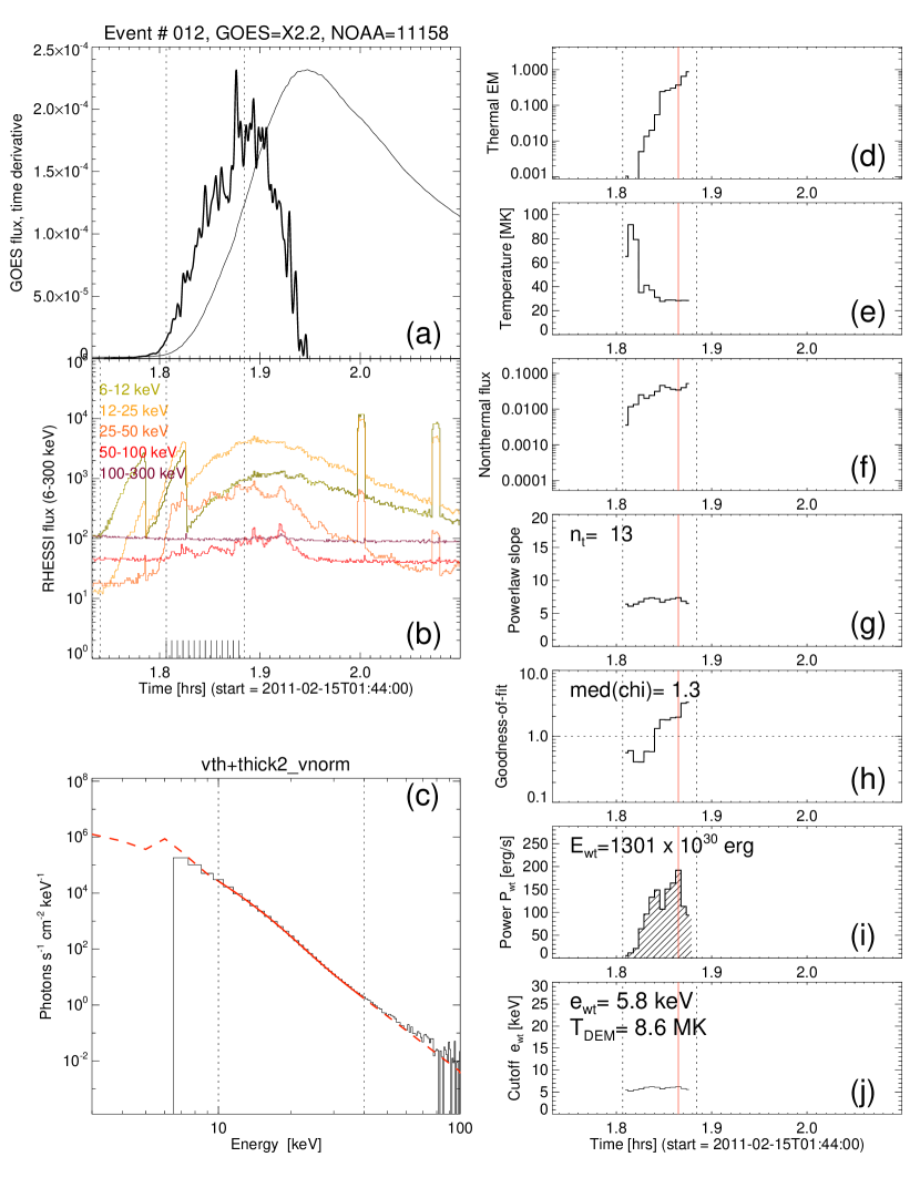
Figure 3: The data analysis of a large flare event #12, GOES X2.2-class, observed on 2011-Feb-15, 01:44 UT, otherwise similar representation as in Figs. 1 and 2.

From the same comprehensive catalog of 399 M and X-class flares observed with SDO during 2010-2014, used in the first two studies of our global flare energetics project, we will analyze all events that have been simultaneously observed in hard X-rays and gamma-rays with RHESSI. The orbit of RHESSI has a duty cycle of $\approx 50\%$, leading to a total of 191 events that have suitable time coverage. In the following we describe the analysis of these events, which are also listed in Table 1 (labeled with identical identification numbers #1$-$399 as used in Papers I and II). We explain the various steps performed in our analysis for three examples shown in Figs. 1-3.

3.1 Spectral Modeling of RHESSI Data with OSPEX

For the measurement of the nonthermal energy ($E_{\mathrm{nt}}$) of electrons during solar flares we use the OSPEX (Object Spectral Executive) software, which is an object-oriented interface for X-ray spectral analysis of solar data, written by Richard Schwartz and others (see RHESSI website http://hesperia.gsfc.nasa.gov/ for a documentation). The OSPEX software allows the user to read RHESSI data, to select and subtract a background, to select time intervals of interest, to select a combination of photon flux model components, and to fit those components to the spectrum in each selected time interval. During the fitting process, the response matrix is used to convert the photon model to the model counts that are fitted to the observed counts. The OSPEX software deals also with changes of attenuator states, decimation, pulse pile-up effects, albedo effects, and provides procedures to calculate the nonthermal energy $(E_{\mathrm{nt}})$ (according to the thick-target model) and the thermal energy ($E_{\mathrm{th}}$) down to energies of $\lower 1.72218pt\hbox{$\;\buildrel>\over{\scriptstyle\sim}\;$}3$ keV.

RHESSI complements spectral information of the differential emission measure (DEM) distribution at the high-temperature side ($T_{e}\lower 1.72218pt\hbox{$\;\buildrel>\over{\scriptstyle\sim}\;$}16$ MK) (Caspi 2010; Caspi and Lin 2010; Caspi et al. 2014), while AIA/SDO provides DEM information at the low-temperature side ($T_{e}\lower 1.72218pt\hbox{$\;\buildrel<\over{\scriptstyle\sim}\;$}16$ MK), as we determined in Paper II. For spectral modeling we are using the two-component model vth+thick2$\_$vnorm, which includes a thermal component at low energies and a (broken) power law function at higher (nonthermal) energies. In our spectral fits we are only interested in the transition from the thermal to the nonthermal spectrum, which can be expressed by an exponential-like plus a single power law function (Eq. 7), and thus we use only the lower power law part of the two-component model vth+thick2$\_$vnorm, while the spectral slope in the upper part was set to a constant ($\delta_{2}=4$). In addition we use calc$\_$nontherm$\_$electron$\_$energy$\_$flux of the OSPEX package to calculate the nonthermal energy flux in the thick-target model.

RHESSI Spectral Fitting Range Selection: In order to obtain a self-consistent measure of the nonthermal energy, which varies considerably during the duration of a flare or among different flares, we have to choose a spectral fitting range that covers a sufficient part of both the thermal and nonthermal components. We choose the maximum energy range $[\varepsilon_{1},\varepsilon_{2}]$, bound by $\varepsilon_{1}=6...10$ keV and $\varepsilon_{2}=20...50$ keV, in which an acceptable (reduced) $\chi^{2}$-value ($\chi<2.0$) is obtained for the spectral fit. The upper bound of the fitting range is mostly constrained by the photon count statistics, which is often too noisy for energies at $\varepsilon_{2}\lower 1.72218pt\hbox{$\;\buildrel>\over{\scriptstyle\sim}\;$}30$ keV during small flares (M-class here), given the time steps of $\Delta t=20$ s chosen throughout. The fitted energy ranges cover also the range of cross-over energies (10-28 keV) found in multi-thermal fitting of energy-dependent time delays (Aschwanden 2007).

As a general criticism, we have to be aware that the nonthermal spectral component could in addition also be confused with a multi-thermal component in the fitted spectral range of $\varepsilon\approx 10-30$ keV (Aschwanden 2007), or with non-uniform ionization effects (Su, Holman, and Dennis 2011), or with return-current losses (Holman 2012).

RHESSI Detector Selection: We used the standard option of OSPEX, where a spectral fit is calculated from the combined counts of a selectable set of RHESSI subcollimaters. RHESSI has 9 (subcollimator) detectors that had originially near-identical sensitivities, but progressively deviate from each other as a result of steady degradation over time due to radiation damage from charged particles. Heating up the germanium restores the lost sensitivity and resolution, and thus five annealing procedures have been applied to RHESSI so far (second anneal at 2010 Mar 16 - May 1; third at 2012 Jan 17 - Febr 22; forth at 2014 Jun 26 - Aug 13; and fifth at 2016 Feb 23 - Apr 23). No science data are collected during the annealing periods. Based on the performance of the individual detector sensitivities, it is general practice to exclude the detectors 2 and 7 in spectral fits. Furthermore, detectors 4 and 5 are considered as unreliable after January 2012 (Richard Schwartz; private communication). Therefore, we select the set of detectors [1, 3, 4, 5, 6, 8, 9] in spectral fits up to the third anneal in January 2012 (events # 1-126 in Table 1), and the set of [1, 3, 6, 8, 9] after February 2012 (events # 154-395 in Table 1). Omitting detectors 4 and 5 in the latter set of 71 events yields a total nonthermal energy that is by a factor of $q_{\mathrm{det}}=E_{\mathrm{nt}}[1,3,6,8,9]/E_{\mathrm{nt}}[1,3,4,5,6,8,9]=1.3\pm 0.5$ higher.

GOES Time Range and RHESSI Time Resolution: We download the GOES 1-8 Å light curves $F_{\mathrm{GOES}}(t)$ and calculate the time derivative as a proxy for the hard X-ray time profile $F_{\mathrm{HXR}}\approx dF_{\mathrm{GOES}}/dt$, as shown in Figs. 1a ,2a, and 3a. The start time $t_{\mathrm{start}}$, peak time $t_{\mathrm{peak}}$, and end time $t_{\mathrm{end}}$ are defined from the NOAA/GOES catalog. We compute consecutive spectra in time steps of $\Delta t=20$ s. Note that RHESSI is a spinning spacecraft with a period of 4 s, which does not cause any modulation effects for 20 s time integrations.

RHESSI Quick-Look Data: In a next step we inspect the RHESSI quick-look time profiles (Figs. 1b, 2b, 3b), which show photon counts in 5 different energy channels in the range of 6-300 keV. Based on these RHESSI time profiles we select time intervals for background subtraction. Generally we select a time interval at flare start as the background interval (in 90%), and subtract this preflare spectrum for the entire flare time interval. Only in a few cases (10%) where the preflare flux is higher than the postflare flux, we choose a time interval at flare end for background subtraction. The RHESSI quick-look data show changes in the attenuator state (e.g., Figs.2b, 3b), which are automatically handled in most time intervals with the OSPEX software, unless there is a change in the attenuator state during a selected time interval itself, in which case this time interval is removed from the spectral analysis. The quick-look data show occasionally data gaps that are caused when RHESSI enters spacecraft night in its near-Earth orbit. If the data gap does not occur during the flare peak of hard X-ray emission, we still include the event in the analysis, as long as the time interval of dominant nonthermal HXR emission is covered (such as event #219 in Fig. 2b).

OSPEX Spectral Fitting: For spectral fitting we perform first a semi-calibration and store the detector response matrix (DRM), and then run a spectral fit with the fit function vth+thick2$\_$vnorm using the OSPEX software, optimizing the following model fit parameters (for each time interval $t$):

$EM(t)$	= Emission measure in units of $10^{49}$ cm-3
$T_{e}(t)$	= plasma temperature in units of keV (1 keV=11.6 MK)
$A(t)$	= photon flux at $\varepsilon=50$ keV
$\delta(t)$	= negative power law index of electron spectrum
$e_{c}(t)$	= low-energy cutoff

Examples of spectral fits are shown in Figs. 1c, 2c, and 3c, fitted at the time of the peak power $P_{\mathrm{co}}(t)$ (indicated with red vertical lines in Figs. 1, 2, and 3). The best-fit spectrum yields a cross-over energy $e_{\mathrm{co}}$ between the thermal and nonthermal spectral component. Alternatively, the warm-target model of Kontar et al. (2015) yields a low-energy cutoff value $e_{\mathrm{wt}}$. The fitted energy ranges are listed in Table 1 and are indicated with dotted vertical lines in Figs. 1g, 2g, and 3g. The goodness-of-fit is quantified with the $\chi^{2}$-value criterion. In case of bad fits of the $\chi^{2}$-values ($\chi>2$) we changed either the fitted energy range (in 13%), the selected interval for background subtraction (10%), or the fitted time range (5%).

4 RESULTS

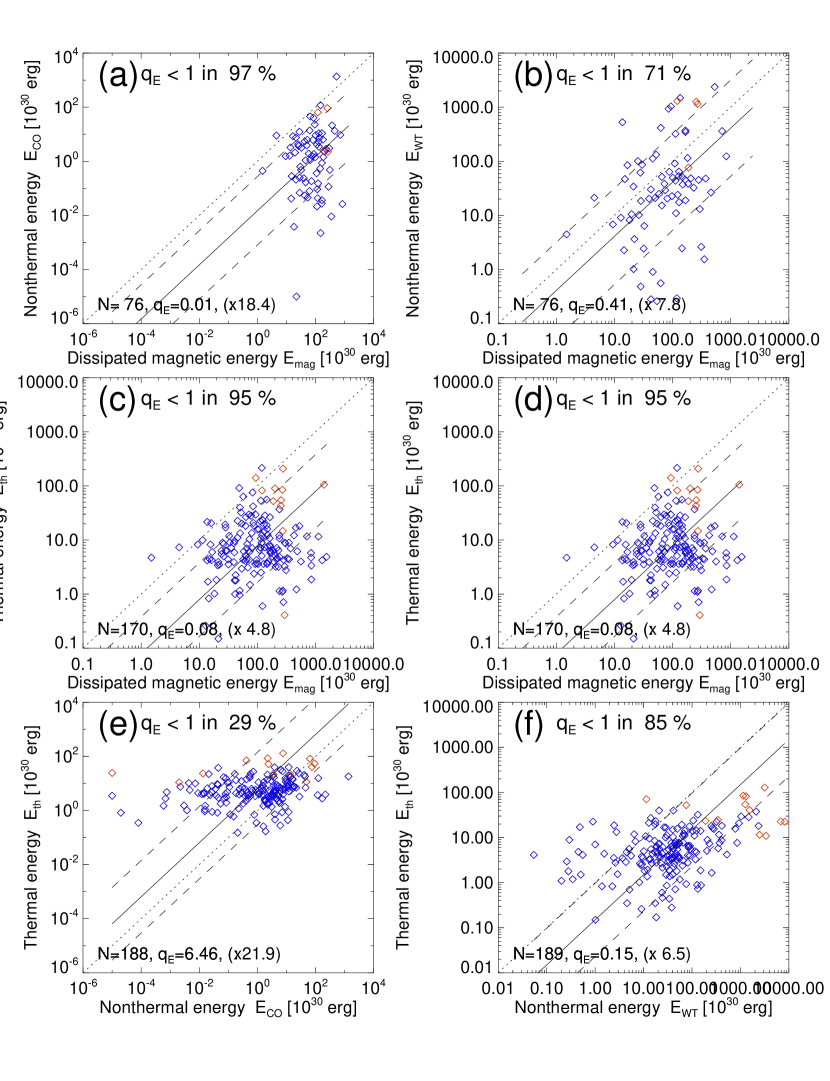
Figure 6: Scatter plots are shown between the dissipated magnetic energies $E_{mag}$ (calculated in Paper 1), the thermal energies $E_{th}$ (calculated in Paper 2), and the non-thermal energies calculated here, using the cross-over method (left panels a,e) and the warm-target model (right panels b,f). The mean ratios (by averaging the logarithmic values) (solid lines) are indicated in each panel with the standard deviations (two dashed lines and multiplier marked with $\times$), and the unity ratio (dotted line). The color code indicates X-class (red) and M-class flares (blue).

The numerical values of the main results of the low energy cutoffs $e_{c}$ (which we label as $e_{\mathrm{co}}$ in the cross-over method, and as $e_{\mathrm{wt}}$ in the warm-target method), and the nonthermal energy $E_{\mathrm{nt}}$ for the analyzed 191 events are listed in Table 1, while scatter plots and distributions are shown in Figs. 4-8.

4.1 Time Evolution of Flares

Three examples of analyzed flare events are shown in Figs. 1, 2, and 3, including one of the smallest events (Fig. 1: #387, GOES M1.0 class), an event with multi-peak characteristics (Fig. 2; #219, GOES M2.0 class), and one of the largest events (Fig. 3; #12, GOES X2.2 class). In all three cases we show the time evolution of the most important fit parameters in the various panels (d through j) of Figs. 1-3: (d) the thermal emission measure $EM(t)$; (e) the temperature evolution $T_{e}(t)$; (f) the nonthermal photon flux $I_{\mathrm{nt}}(t)$ at 50 keV; (g) the power law slope $\delta(t)$; (h) the goodness-of-fit $\chi(t)$; (i) the nonthermal power $P_{\mathrm{wt}}(t)$ using the low cutoff energy based on the warm-target model (Section 2.3); and (j) the low-energy cutoff $e_{\mathrm{wt}}(t)$ of the warm-target model. In the examples shown in Figs. 1, 2 and 3 we see that the thermal emission measure $EM(t)$ increases during the rise time of the GOES flux, while the temperature $T_{e}(t)$ decreases, which indicates both density increases due to chromospheric evaporation as well as subsequent plasma cooling during the impulsive flare phase. Since multiple heating and cooling cycles overlap during a flare, we see both effects simultaneously. The cases shown in Figs. 1, 2 and 3 show also that the nonthermal flux $I_{\mathrm{nt}}(t)$ (Figs. 1f, 2f, 3f) and the power $P_{\mathrm{wt}}(t)$ (Figs. 1i, 2i, 3i) are correlated with the GOES time derivative (Figs. 1a, 2a, 3a).

4.2 Goodness-of-Fit

The goodness of the spectral fits computed with the OSPEX code is specified with the $\chi^{2}$-criterion, based on the least-square difference between the theoretical spectral model (isothermal plus power law nonthermal function) and the observed counts in the fitted energy range [$\varepsilon_{1}$-$\varepsilon_{2}$]. The fitted energy time interval (with a resolution of 1 keV) has about $n_{\mathrm{bin}}\approx 30-10=20$ energy bins, while the model has four ($n_{\mathrm{par}}=4)$ free parameters $(EM,T_{e},A_{50},\delta)$, yielding a degree of freedom $n_{\mathrm{free}}=n_{\mathrm{bin}}-n_{\mathrm{par}}\approx 20-4=16$. In our spectral analysis of 191 flare events we performed spectral fits, with an average of $n_{t}\approx 27$ time steps per event, amounting to a total of $N_{\mathrm{spec}}\approx 191\times 27=5157$ spectral fits. The values $\chi(t)$ of three events are shown in Figs. 1h, 2h, and 3h. The median values of these three events are $\chi=1.4,1.0$, and 1.3. We obtained in all 191 events a median goodness-of-fit value of $\chi<2$, after adjustment of the fitted energy range if necessary. The mean and standard deviations of the median $\chi^{2}$-values of all 191 events is $\chi=1.2\pm 0.4$, which indicates that the fitted spectral model is adequate in the chosen fitted energy range. Of course, if one particular model, such as the two-component thermal-nonthermal model chosen here (Eq. 7), is found to be consistent with the data according to an acceptable goodness-of-fit criterion, it does not rule out alternative models. For instance, the thermal component is often modeled with an iso-thermal (single-temperature) spectrum, while a multi-thermal power law function was found to fit the thermal flare component in most flares equally well (Aschwanden 2007).

4.3 Temperature Definitions

A representative value for the electron temperature during a flare can be defined in various ways. In paper II we measured the peak temperature $T_{\mathrm{AIA}}$ of the differential emission measure (DEM) distribution at the peak time of the flare, as well as the emission measure-weighted temperature $T_{w}$ (Eq. 13 in Paper II), which approximately characterizes the “centroid” of the (logarithmic) DEM function. The mean ratio of these two temperature values was found to be $q_{T}=T_{\mathrm{AIA}}/T_{w}=0.31$ within a standard deviation by a factor of $2.0$ (Fig. 4, left panel). The emission measure-weighted temperature $T_{w}$ is generally found to be higher, because near-symmetric DEM functions as a function of the logarithmic temperature are highly asymmetric on a linear temperature scale, with a centroid that is substantially higher than the logarithmic centroid.

On the other hand, spectral fits of RHESSI data with an isothermal component are known to have a strong bias towards the highest temperatures occurring in a flare, because the fitted energy range covers only the high-temperature tail of the DEM distribution function (Battaglia et al. 2005; Ryan et al. 2014; Caspi et al. 2014). A statistical study demonstrated that the high-temperature bias of RHESSI by fitting in the photon energy range of $\varepsilon\approx 6-12$ keV amounts to a factor of $T_{R}/T_{\mathrm{AIA}}=1.9\pm 1.0$ (Ryan et al. 2014). Here we find that all RHESSI temperatures averaged during each flare are found in a range of $T_{R}=16-40$ MK, which is about equal to the emission measure-weighted temperature, i.e., $T_{R}/T_{w}=0.90$ within a factor of 1.4 (Fig. 4, right panel). The 1-$\sigma$ ranges (containing 67% of the values) of the various temperature definitions are $T_{\mathrm{AIA}}\approx 3-14$ MK, $T_{w}\approx 20-30$ MK, and $T_{R}\approx 19-28$ MK. So, we should keep these different temperature definitions in mind when we calculate the low-energy cutoff $e_{c}(t)$ as a function of the RHESSI temperature $T_{R}(t)$ (Eq. 8 for the warm-target model).

The most decisive parameter in the determination of the nonthermal energy $E_{nt}$ is the low-energy cutoff $e_{c}$ (Eq. 4), which is directly proportional to the temperature $T_{e}$ in the warm target (Eq. 8). What is the most likely temperature of the warm target? The relevant temperature is a mixture of pre-flare plasma temperatures and upflowing evaporating flare plasma. In the absence of a sound model, we resort to the mean value of the DEM peak temperatures determined in flaring active regions, as determined with AIA in Paper II, yielding a mean value of $T_{AIA}=8.8\pm 6.0$ MK (Fig. 4 left panel), averaged over $N=380$ M and X-class flare events. For the subset of 191 flare events observed with RHESSI, this mean value is $T_{e}=8.6$ MK, or $k_{B}T_{e}=0.74$ keV. Note that a deviation of the plasma temperature by a factor of two will result into a deviation in the determination of the nonthermal energy $E_{nt}$ by about an order of magnitude (using a power law with a typical slope of $\gamma\approx 4$ in Eqs. 3 and 4).

4.4 Nonthermal Energy Parameters

The nonthermal energy in electrons, calculated as a time integral $E_{\mathrm{nt}}$ (Eq. 4), using the low-energy cutoff according to the warm thick-target model $e_{\mathrm{wt}}(t)$ (Section 2.3; Eq. 8), or alternatively the thermal/nonthermal cross-over energy $e_{\mathrm{co}}(t)$ (Section 2.2), is the main objective of this study. Examples of the time evolution of the nonthermal parameters [$A(t),\delta(t)$, $e_{\mathrm{co}}(t)$, $e_{\mathrm{wt}}(t)$] and the resulting nonthermal energies $dE_{\mathrm{nt}}(t)$ are shown in Figs. 1-3. In Fig. 5 we show statistical results of these parameters. Investigating the dependence of these parameters on the flare temperature $T_{R}$ we find that both the low-energy cutoff energy $e_{\mathrm{wt}}$ (Fig. 5a) as well as the nonthermal (warm-target) energy $E_{\mathrm{nt}}$ (Fig. 5b) are uncorrelated with the RHESSI temperature.

If we use the thermal-nonthermal cross-over method to estimate the low-energy cutoff, we find a systematically higher value, $e_{\mathrm{co}}\lower 1.72218pt\hbox{$\;\buildrel>\over{\scriptstyle\sim}\;$}e_{\mathrm{wt}}$ (Fig. 5c). Consequently, the nonthermal energy estimated with the cross-over method is systematically lower than the nonthermal energy calculated with the warm-target model (Fig. 5d). This result strongly depends on the assumption of the warm-target temperature. Based on a mean temperature of $T_{e}=8.6$ MK found in the active regions analyzed here, we derive low-energy cutoff energies of $e_{\mathrm{wt}}=6.2\pm 1.6$ keV for the warm-target model, which is significantly lower than the cross-over energies $e_{\mathrm{co}}=21\pm 6$ keV. If we adopt the warm-target model, we conclude that the cross-over method over-estimates the low-energy cutoff and under-estimates the nonthermal energies.

4.5 Comparison of Magnetic, Nonthermal, and Thermal Energies

In Fig. 6 we show scatterplots of the nonthermal energy $E_{\mathrm{nt}}$ measured here with other forms of previously determined energies, such as the magnetic energy $E_{\mathrm{mag}}$ (Paper I) and the (total pre-impulsive and post-impulsive) thermal energies $E_{\mathrm{th}}$ (Paper II). The energy ratios are characterized with the means of the logarithmic energies in the following. The ratios between the three forms of energies are shown separately for the cross-over method in the left-hand panels of Fig. 6, and for the warm-target model in the right-hand panels of Fig. 6.

The ratios between the nonthermal energies and the magnetically dissipated energy is $E_{\mathrm{co}}/E_{\mathrm{mag}}=0.01$ for the cross-over method, or $E_{\mathrm{wt}}/E_{\mathrm{mag}}=0.41$ for the warm-target model, respectively. Thus, the warm-target model yields ratios that are closer to unity, which is expected in terms of magnetic reconnection processes, where most of the magnetic energy is converted into particle acceleration. We find that the dissipated magnetic energy is sufficient to supply the energy in nonthermal particles in 71% for the warm-target model, or in 97% for the cross-over model (Figs. 6a and 6b).

The ratios between the thermal energies and the magnetically dissipated energy is $E_{\mathrm{th}}/E_{\mathrm{mag}}=0.08$ for both the cross-over or the warm-target model (Fig. 6c and 6d). We find that the dissipated magnetic energy is sufficient to supply the thermal energy in 95%.

Comparing the thermal with the nonthermal energies, we find a mean a ratio of $E_{\mathrm{th}}/E_{\mathrm{wt}}=0.15$ for the warm-target model, or $E_{\mathrm{th}}/E_{\mathrm{co}}=6.46$ for the cross-over method. We find that the nonthermal energy is sufficient to supply the thermal energy in 85% for the warm-target model (Fig. 6f), but only in 29% for the cross-over method. Thus, the warm-target model yields values that are closer to the expectations of the standard thick-target model, where the thermal energy is entirely produced by the nonthermal energy of precipitating (nonthermal) electrons.

We show the comparison of nonthermal and thermal energies also in form of cumulative size distributions in Fig. 7, for the subset of 75 flare for which all three forms of (magnetic, thermal, nonthermal) energies could be calculated. We find that the nonthermal energy is typically an order of magnitude larger than the thermal energy in the statistical average. Then we find that the nonthermal energy is smaller than the magnetic energy, as expected for magnetic reconnection processes, for smaller flares with energies of $E_{nt}<3\times 10^{32}$ erg. However, we find the opposite results for larger flares, with the nonthermal energy exceeding the magnetically dissipated energy, for large events with $E_{nt}>3\times 10^{32}$ erg. Since the uncertainties in nonthermal energies are about an order of magnitude and the dissipated magnetic energy exceeds the nonthermal energy in 71% (Fig. 6b), we suspect that the largest nonthermal energies are over-estimated, which would indicate that a higher value of the low-energy cutoff or a higher flare plasma temperature (than the mean active region temperature $T_{e}=8.6$ MK used here) could ameliorate the over-estimated nonthermal energies.

We compare the occurrence frequency distributions of magnetic, nonthermal, and thermal energies, as well as those of the direct RHESSI observables: the peak counts $P$, total counts $C$, and durations $D$ (Fig. 8). As a caveat, we have to be aware that these values for $P$ and $C$ are obtained from the online RHESSI flare catalog, and thus are not well-calibrated, as they do not take attenuation or decimation into account. Nevertheless, taking these raw values, the magnetic and thermal energies have similar power law slopes of $\alpha\approx 2.0$, while the nonthermal energies have a slightly flatter slope of $\alpha_{\mathrm{nt}}=1.55\pm 0.11$, which can be compared with a previous study, where a power law slope of $\alpha_{\mathrm{nt}}=1.53\pm 0.02$ was found (Crosby et al. 1993). The latter study is actually based on larger statistics, containing 2878 flare events observed with HXRBS/SMM during 1980-1982 (Crosby et al. 1993), but with a higher assumed low-energy cutoff of $e_{c}>25$ keV.

5 DISCUSSION

5.1 Energy Partition in Flares

While we determined the dissipated magnetic energies $E_{\mathrm{mag}}$ (Paper I; called $E_{\mathrm{diss}}$ therein), thermal energies $E_{\mathrm{th}}$ (Paper II), and the nonthermal energies $E_{\mathrm{nt}}$, we can ask now the question how the energy partition from primary to secondary energy dissipation works in solar flares. Many solar flare models are based on a magnetic reconnection process, where a stressed non-potential magnetic field becomes unstable and undergoes a reconfiguration towards a lower magnetic energy state, releasing during this process some amount $E_{\mathrm{mag}}=q_{\mathrm{diss}}E_{\mathrm{free}}$ of the magnetic free energy $E_{\mathrm{free}}$ (defined by the difference between the non-potential and the potential energy, $E_{\mathrm{free}}=E_{\mathrm{np}}-E_{p}$). Excluding alternative energy sources, we hypothesize that this dissipated magnetic energy $E_{\mathrm{mag}}$ is considered to be the entire available primary energy input, while other energy conversion processes represent secondary steps that need to add up in the energy budget,

$$E_{\mathrm{mag}}=(E_{\mathrm{nt}}+E_{\mathrm{cme}}+...)>E_{\mathrm{nt}}\ ,$$ (9)

such as the nonthermal energy $E_{\mathrm{nt}}$ that goes into acceleration of particles, or the energy $E_{\mathrm{cme}}$ to accelerate an accompanying coronal mass ejection (CME). The nonthermal energy $E_{\mathrm{nt}}$ may be further subdivided into energies in electrons $E_{\mathrm{nt,e}}$ and ions $E_{\mathrm{nt,i}}$,

$$E_{\mathrm{nt}}=(E_{\mathrm{nt,e}}+E_{\mathrm{nt,i}}+...)>E_{\mathrm{nt,e}}\ ,$$ (10)

while the CME energy $E_{\mathrm{cme}}$ consists of the kinetic energy $E_{\mathrm{kin}}$ and the gravitational potential energy $E_{\mathrm{grav}}$, and part of it may be converted into acceleration of particles in the interplanetary CME shock ($E_{\mathrm{nt,cme}}$), which are particularly present in solar energetic particle (SEP) events,

$$E_{\mathrm{cme}}=E_{\mathrm{kin}}+E_{\mathrm{grav}}+E_{\mathrm{nt,cme}}+...\ .$$ (11)

We have to be careful to avoid double-counting of secondary energies, because there may be some tertiary energy conversion processes, such as heating of chromospheric plasma according to the thick-target bremsstrahlung model, $E_{\mathrm{th}}$, while upgoing nonthermal particles escape into interplanetary space, carrying an energy of $E_{\mathrm{nt,esc}}$,

$$E_{\mathrm{nt}}=(E_{\mathrm{th}}+E_{\mathrm{nt,esc}}+...)>E_{\mathrm{th}}\ .$$ (12)

Since we have measured only three types of energies so far, $E_{\mathrm{mag}},E_{\mathrm{nt}}$, and $E_{\mathrm{nt}}$, we can test only the inequalities given on the righthand-side of Eqs. (9) and (12) at this point.

Based on the nonthermal energies in electrons determined in this work we can answer the question whether the so far measured magnetic energy is sufficient to accelerate the electrons observed in hard X-rays, i.e., $E_{\mathrm{mag}}>E_{\mathrm{nt}}$, as expected for magnetic reconnection models. Relying on the warm-target model we found that 41% of the dissipated magnetic energy (with a standard deviation of about an order of magnitude) is converted into acceleration of nonthermal electrons, or a total amount of $\approx 82\%$ for both electrons and ions in the case of equipartition, while the rest is available to accelerate CMEs. There are few statistical estimates of the flare energy budget in literature (besides the work of Emslie et al. 2012; Warmuth and Mann 2016). One early study quoted that the nonthermal energy in electrons $>20$ keV contains 10-50% of the total energy output for the August 1972 flares (Lin and Hudson 1976; Hudson and Ryan 1995), which is consistent with our result of 41% within the measurement uncertainties.

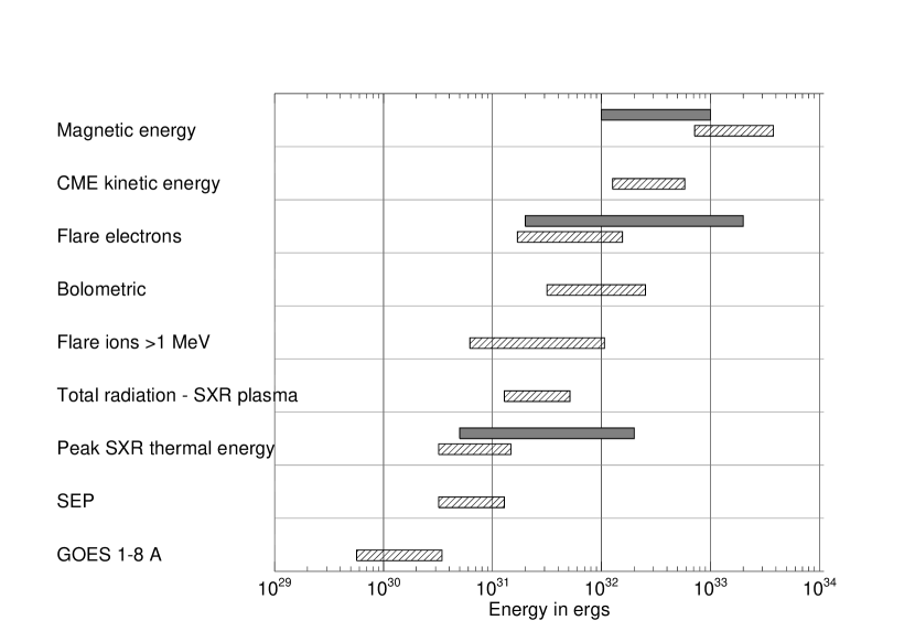
Figure 9: Bar chart showing the logarithmic ranges of energy distributions according to the study of 38 events in Emslie et al. (2012) (hatched boxes). For comparison, the magnetic energies in 172 events (Aschwanden et al. 2014), the thermal energies in 391 events (Aschwanden et al. 2015), and the nonthermal energies in this study here are shown (all in grey boxes). The grey boxes exclude incompletely-sampled ranges.

Comparing the energy ranges determined in this global flare energetics project with those obtained from 38 events in Emslie et al. (2012), we find higher amounts of nonthermal flare electron energies in the statistical average, covering the range of $E_{\mathrm{nt}}\approx(20-2000)\times 10^{30}$ erg (Fig. 9), which is mostly accounted for by a lower value of the low-energy cutoff predicted by the warm-target model (Kontar et al. 2015) for some events, while cutoff energies with the highest acceptable value of the $\chi^{2}$ was used in Emslie et al. (2012). The magnetically dissipated energies appear to be over-estimated by an order of magnitude (Fig. 9) in Emslie et al. (2012), based on the ad hoc assumption that the dissipated energy amounts to 30% of the potential field energy therein (Paper I). On the other hand, the thermal energies appear to be underestimated by at least an order of magnitude (Fig. 9) in Emslie et al. (2012) due to the isothermal approximation, as discussed in Paper II.

5.2 Insufficiency of the Thick-Target Model?

A second question we can answer is whether the nonthermal energy in electrons is sufficient to heat the flare plasma by the chromospheric evaporation process, as expected in the thick-target model according to the Neupert effect (Dennis and Zarro 1993), which requires $E_{\mathrm{nt}}>E_{\mathrm{th}}$. Based on the warm-target model we found a mean (logarithmic) ratio of $E_{\mathrm{th}}=0.15\ E_{\mathrm{nt}}$ (Fig. 6f). The fraction of flares that have a thermal energy less than the nonthermal energy, as expected in the standard thick-target model, amounts in our analysis to $\approx 85\%$ for the warm-target method, or $\approx 29\%$ for the cross-over model.

This means that the thick-target model could be insufficient to supply enough energy to explain the thermal energy produced by the chromospheric evaporation process in about 15% of the flares for the warm-target model, or in 71% for the cross-over model. Thus, the cross-over model would pose a series problem for the thick-target model. The insufficiency of the thick-target model has been addressed as a failure of the theoretical Neupert effect (Veronig et al. 2005; Warmuth and Mann 2016), which invokes testing of the correlation between the electron beam power (from RHESSI) and the time derivative of the thermal energy heating rate (from GOES). From such study it was concluded that (1) fast electrons are not the main source of soft X-ray plasma supply and heating, (2) the beam low cutoff energy varies with time, or (3) the theoretical Neupert effect is strongly affected by the source geometry (Veronig et al. 2005). If the thermally dominated flares cannot be fully explained by the thick-target model, additional heating sources besides precipitating electrons would be required. The most popular alternative to the thick-target model is heating by thermal conduction fronts (Brown et al. 1979; Batchelor et al. 1985; Emslie and Brown 1980; Smith and Harmony 1982; Smith and Brown 1980; Reep et al. 2016). Other forms of direct heating (for an overview see chapter 16 in Aschwanden 2004) occur via (1) resistive or Joule heating processes, such as anomalous resistivity heating (Duijveman et al. 1981; Holman 1985; Tsuneta 1985), ion-acoustic waves (Rosner et al. 1978b), electron ion-cyclotron waves (Hinata 1980), (2) slow-shock heating (Cargill and Priest 1983; Hick and Priest 1989), (3) electron beam heating by Coulomb collisional loss in the corona (Fletcher 1995, 1996; Fletcher and Martens 1998), (4) proton beam heating by kinetic Alfvén waves (Voitenko 1995, 1996), or (5) inductive current heating (Melrose 1995, 1997).

The thick-target model fails to explain the observed amount of thermal energy only in a small number of flares for the warm-target model, while it is a larger number of events for the cross-over method. However, it is more likely that the cross-over method over-estimates the low-energy cutoff, which under-estimates the nonthermal energies, while the physics-based warm-target model leads to higher nonthermal energies, in which case the problem with the insufficiency of the thick-target model goes away.

5.3 Nonthermal Low-Energy Cutoff in Flares

We outlined two different methods to infer a low-energy cutoff. The first method consists in measuring the cross-over between the fitted thermal and nonthermal spectral components, which yields an upper limit on the low-energy cutoff, but a statistical test demonstrates that the obtained values ($e_{\mathrm{co}}=21\pm 6$ keV) are significantly higher than those obtained from the warm-target model ($e_{\mathrm{wt}}=6.2\pm 1.6$ keV). There are pros and cons for each method. The cross-over method requires a dominant thermal component, which is not always detectable in the spectrum, in which case the cross-over energy has a large uncertainty. The warm-target model requires the measurement of the (warm) flare temperature, which is measured at lower values from DEMs at EUV wavelengths than from hard X-ray spectra observed with RHESSI. Moreover, the spatial temperature distribution is very inhomogeneous and the location with the dominant temperature component relevant for the warm-target collisional energy loss may be a mixture of colder pre-flare plasma in active regions and heated evaporating flare plasma at the location of instantaneous electron precipitation. In summary, the value of the low-energy cutoff is strongly dependent on the assumed warm-target temperature, for which no physical model is established yet.

In this study we investigated also the temporal evolution of the low energy cutoff $e_{c}(t)$, for instance as shown in Fig. 1j, 2j, and 3j, but we do not recognize a systematic pattern how the evolution of this low-energy cutoff is related to other flare parameters.

6 CONCLUSIONS

The energy partition study of Emslie et al. (2012) was restricted to 38 large solar eruptive events (SEE). In a more comprehensive study on the global flare energetics we choose a dataset that contains the 400 largest (GOES M and X-class) flare events observed during the first 3.5 years of the SDO era. Previously we determined the dissipated magnetic energies $E_{\mathrm{mag}}$ in these flares based on fitting the vertical-current approximation of a nonlinear force-free field (NLFFF) solution to the loop geometries detected in EUV images from SDO/AIA, a new method that could be applied to 177 events with a heliographic longitude of $\leq 45^{\circ}$ (Paper I). We also determined the thermal energy $E_{\mathrm{th}}$ in the soft X-ray and EUV-emitting plasma during the flare peak times based on a multi-temperature differential emission measure DEM forward-fitting method to SDO/AIA image pixels with spatial synthesis, which was applicable to 391 events (Paper II). In the present study we determined the nonthermal energy $E_{\mathrm{nt}}$ contained in accelerated electrons based on spectral fits to RHESSI data using the OSPEX software, which was applicable to 191 events. The major conclusions of the new results emerging from this study are:

1. The (logarithmic) mean energy ratio of the nonthermal energy to the total magnetically dissipated flare energy is found to be $E_{\mathrm{nt}}/E_{\mathrm{mag}}=0.41$, with a logarithmic standard deviation corresponding to a factor of $\approx 8$, which yields an uncertainty $\sigma/\sqrt{N}=0.41/\sqrt{191}=0.03$ for the mean, i.e., $E_{\mathrm{nt}}/E_{\mathrm{mag}}=0.41\pm 0.03$. The majority ($\approx 85\%$) of the flare events fulfill the inequality $E_{\mathrm{nt}}/E_{\mathrm{mag}}<1$, which suggests that magnetic energy dissipation (most likely by a magnetic reconnection process) provides sufficient energy to accelerate the nonthermal electrons detected by bremsstrahlung in hard X-rays. Our results yield an order of magnitude higher electron acceleration efficiency than previous estimates, i.e., $E_{\mathrm{nt}}/E_{\mathrm{mag}}=0.03\pm 0.005$ (with $N=37$, Emslie et al. 2012).

2. The (logarithmic) mean of the thermal energy $E_{\mathrm{th}}$ to the nonthermal energy $E_{\mathrm{nt}}$ is found to be $E_{\mathrm{th}}/E_{\mathrm{nt}}=0.15$, with a logarithmic standard deviation corresponding to a factor of $\approx 7$. The fraction of flares with a thermal energy being smaller than the nonthermal energy, as expected in the thick-target model, is found to be the case for $\approx 85\%$ only. Therefore, the thick-target model is sufficient to explain the full amount of thermal energy in most flares, in the framework of the warm-target model. The cross-over method shows the opposite tendency, but we suspect that the cross-over method over-estimates the low energy cutoff and under-estimates the nonthermal energies. Previous estimates yielded a similar ratio, i.e., $E_{\mathrm{th}}/E_{\mathrm{nt}}=0.15$ (Emslie et al. 2012).

3. A corollary of the two previous conclusions is that the thermal to magnetic energy ratio is $E_{\mathrm{th}}/E_{\mathrm{mag}}=0.08$. A total of $95\%$ flares fulfils the inequality $E_{\mathrm{nt}}/E_{\mathrm{mag}}<1$, indicating that all thermal energy in flares is supplied by magnetic energy. Previous estimates were a factor of 17 lower, i.e., $E_{\mathrm{th}}/E_{\mathrm{mag}}=0.0045$ (Emslie et al. 2012), which would imply a very inefficient magnetic to thermal energy conversion process.

4. The largest uncertainty in the calculation of nonthermal energies, the low-energy cutoff, is found to yield different values for two used methods, i.e., $e_{\mathrm{wt}}=6.2\pm 1.6$ keV for the warm thick-target model, versus $e_{\mathrm{co}}=21\pm 6$ keV for the thermal/nonthermal cross-over method. The calculation of the nonthermal energies is highly sensitive to the value of the low-energy cutoff, which strongly depends on the assumed (warm-target) temperature.

5. The flare temperature can be characterized with three different definitions, for which we found the following ($67\%$-standard deviation) ranges: $T_{\mathrm{AIA}}\approx 3-14$ MK for the AIA DEM peak temperature, $T_{w}\approx 20-30$ MK for the emission measure-weighted temperatures, and $T_{R}\approx 17-36$ MK for the RHESSI high-temperature DEM tails. The median ratios are found to be $T_{\mathrm{AIA}}/T_{w}=0.31$ and $T_{R}/T_{w}=0.90$. The mean active region temperature evaluated from DEMs with AIA, $T_{e}=8.6$ MK, is used to estimate the low-energy cutoff $e_{c}$ of the nonthermal component according to the warm-target model, i.e., $e_{c}\approx\delta(k_{B}T_{R})$. The low-energy cutoff $e_{c}$ of the nonthermal spectrum has a strong functional dependence on the temperature $T_{R}$.

In summary, our measurements appear to confirm that the magnetically dissipated energy is sufficient to explain thermal and nonthermal energies in solar flares, which strongly supports the view that magnetic reconnection processes are the primary energy source of flares. The nonthermal energy, which represents the primary energy source of the thick-target model, is sufficient to explain the full amount of thermal energies in 71% of the flares, according to the novel warm-target model (Kontar et al. 2011). However, the derived nonthermal energies are highly dependent on the the assumed temperature in the warm-target plasma, for which a sound physical model should be developed (see for instance Appendix A and B), before it becomes a useful tool to estimate the low-energy cutoff of nonthermal energy spectra. Future studies of this global flare energetics project may also quantify additional forms of energies, such as the kinetic energy in CMEs, and radiated energies in soft X-rays, EUV, and white-light (bolometric luminosity).

APPENDIX A : Collisional Time-of-Flight Model

We can derive a collisional time-of-flight model for the thermal/non-thermal cross-over energy that is complementary to the warm-target model of Kontar et al. (2015). For stochastic acceleration models, where particles gain and lose energy randomly, the collisional deflection time yields an upper time limit during which a particle can be efficiently accelerated. The balance between acceleration and collisions can lead to the formation of a kappa-distribution according to some solar flares models (Bian et al. 2014). For solar flares, we can thus estimate the cross-over energy between collisional and collisionless electrons by setting the collisional deflection time $t_{\mathrm{defl}}$,

$$t_{\mathrm{defl}}\approx 0.95\times 10^{8}\left({e_{\mathrm{keV}}^{3/2}\over n_{e}}\right)\left({20\over\ln\Lambda}\right)\ ,$$

where $\ln\Lambda\approx 20$ is the Coulomb logarithm, equal to the (relativistic) time-of-flight propagation time between the coronal acceleration site and the chromospheric thick-target energy loss site,

$$t_{\mathrm{TOF}}={L_{\mathrm{TOF}}\over v}={L_{\mathrm{TOF}}\over\beta c}\ ,$$

where the relativistic speed $\beta=v/c$,

$$\beta=\sqrt{1-{1\over\gamma^{2}}}\ ,$$

is related to the kinetic energy $e_{\mathrm{kin}}$ of the electron by

$$e_{\mathrm{kin}}=m_{e}c^{2}(\gamma-1)=511\ (\gamma-1)\ {\rm[keV]}\ ,$$

where $\gamma$ represents here the relativistic Lorentz factor (not to be confused with the spectral slope of the photon spectrum used above, i.e., Eq. 1). So, setting these two time scales equal,

$$t_{\mathrm{defl}}=t_{\mathrm{TOF}}\ ,$$

yields the relationship, using $\ln\Lambda\approx 20$,

$$(\gamma-1)^{3/2}(1-{1\over\gamma^{2}})^{1/2}={L_{\mathrm{TOF}}\ n_{e}\over 0.95\times 10^{8}\times 511^{3/2}\ c}\ .$$

Using the low-relativistic approximation (for $\gamma\lower 1.72218pt\hbox{$\;\buildrel>\over{\scriptstyle\sim}\;$}1$),

$$(\gamma-1)^{3/2}(1-{1\over\gamma^{2}})^{1/2}=(\gamma-1)^{3/2}{(\gamma-1)^{1/2}(\gamma+1)^{1/2}\over\gamma}={(\gamma-1)^{2}(\gamma+1)^{1/2}\over\gamma}\approx(\gamma-1)^{2}\sqrt{2}\ ,$$

we obtain,

$$(\gamma-1)^{2}\ \sqrt{2}\approx 0.003\times\left({L_{\mathrm{TOF}}\over 10^{9}\ {\rm cm}}\right)\left({n_{e}\over 10^{11}\ {\rm cm}^{-3}}\right)\quad{\rm[keV]}\ .$$

and by inserting $(\gamma-1)=e_{c}/511$ keV from Eq. (A4) we find the cross-over energy $e_{c}\approx e_{\mathrm{kin}}$ can be explicitly expressed as

$$e_{c}\approx 24\left({L_{\mathrm{TOF}}\over 10^{9}\ {\rm cm}}\right)^{1/2}\left({n_{e}\over 10^{11}\ {\rm cm}^{-3}}\right)^{1/2}\quad{\rm[keV]}\ .$$

This expression requires the measurement of a mean length scale $L_{\mathrm{TOF}}$ of flare loops and an average electron density $n_{e}$ where electrons propagate.

Turning the argument around predicts a time-of-flight distance $L_{\mathrm{TOF}}\propto e_{c}^{2}/n_{e}$ as a function of the low-energy cutoff $e_{c}$, which is a similar concept that has been applied to model the size $L$ of the acceleration region as a function of the electron energy $e$, i.e., $(L-L_{0})\propto e^{2}/n_{e}$ (Guo et al. 2012a,b; 2013; Xu, Emslie, and Hurford 2008).

APPENDIX B : The Rosner-Tucker-Vaiana Model

At the peak time of a flare, an energy balance between plasma heating and cooling occurs at the turnover point of the temperature maximum (Aschwanden and Tsiklauri 2009), which corresponds to the scaling law of Rosner, Tucker, and Vaiana (1978a) that was originally applied to steady-state heating of coronal loops, where an energy balance between the heating rate and the conductive and radiative cooling time is assumed. The RTV scaling law, $T^{3}\propto pL$, can be expressed in terms of the ideal gas pressure $p=3n_{e}k_{B}T$, which yields for the loop apex temperature $T_{\mathrm{RTV}}$,

$$T_{\mathrm{RTV}}=0.0011\ (n_{e}L_{\mathrm{RTV}})^{1/2}\ .$$

The loop half length and time-of-flight distance scale approximately with the flare size, $L_{\mathrm{TOF}}\approx L_{\mathrm{RTV}}\approx L$. Interestingly, the parameter combination $(n_{e}L)^{1/2}$ occurs also in the expression for the collisional low-energy cutoff (Eq. A9), so that we can insert the RTV scaling law and obtain an expression for the low-energy cutoff energy $e_{c}$ that depends on the temperature $T_{\mathrm{RTV}}$ only,

$$e_{c}\approx 25\ (k_{B}T_{\mathrm{RTV}})\quad{\rm[keV]}\ ,$$

which is similar to the result of the warm-target model (Eq. 8). However, while the warm-target model is applied to the evaporating upflowing flare plasma, which has temperatures of $T_{e}\approx 10-25$ MK, the collisional deflection model should be applied to the temperature of the cooler preflare loops, where the accelerated particles propagate from the acceleration site to the thick-target site. These cooler preflare loops may have typical coronal temperatures of $T_{\mathrm{RTV}}\approx 5-6$ MK ($\approx 0.43-0.52$ keV) in active regions (Hara et al. 1992), which predicts then low-energy cutoff energies of $e_{c}=11-13$ keV. If the time-of-flight distance $L_{\mathrm{TOF}}$ is corrected for magnetic twist and the pitch angle of the electrons, the effective time-of-flight distance is about $L_{\mathrm{TOF}}\lower 1.72218pt\hbox{$\;\buildrel<\over{\scriptstyle\sim}\;$}2L$ (Aschwanden et al. 1996), which increases the low-energy cutoff energy by a factor of $\sqrt{2}$, predicting values of $e_{c}=15-18$ keV. Combining Eqs. (8) and (B2), the RTV model predicts a relationship between the preflare temperature $T_{\mathrm{pre}}=T_{\mathrm{RTV}}$ and the (maximum) flare temperature $T_{\mathrm{flare}}$,

$$T_{\mathrm{pre}}\approx T_{\mathrm{flare}}\left({\delta\over 25}\right)\ ,$$

which yields $T_{\mathrm{pre}}\approx(0.12-0.24)\ T_{\mathrm{flare}}$ for a range of spectral slopes $\delta\approx 3-6$. Given the fact that flare temperatures are typically found in the range of $T_{flare}\approx 10-25$ MK, while preflare temperatures amount to typical coronal temperatures in active regions, $T_{pre}\approx 1-4$ MK, we would expect indeed temperature ratios of $T_{pre}/T_{flare}\approx 0.1-0.16$.

APPENDIX C : The Runaway Acceleration Model

Some particle acceleration models involve DC electric fields that accelerate electrons and ions out of the bulk plasma. Since the frictional drag on the electrons decreases with increasing particle velocity ($\nu\propto v^{-3}$), electrons in the initial thermal distribution with a high enough velocity will not be confined to the bulk current, but will be freely accelerated out of the thermal distribution (Kuijpers et al. 1981; Holman 1985), a process that is called runaway acceleration. A thermal electron of velocity $v_{e}$ will run away if the electric field strength is greater than the Dreicer field $E_{D}$,

$$E_{D}={m\over e}v_{e}\nu_{e}\ ,$$

where $m$ is the electron mass, $e$ the electron charge, $v_{e}$ the electron velocity, and $\nu_{e}$ the electron collision frequency. Since the square of the (non-relativistic) speed $v_{e}$ scales with the kinetic energy, $E_{\mathrm{kin}}=(1/2)m_{e}v_{e}^{2}$, the critical runaway energy $E_{\mathrm{ra}}$ can be characterized by the ratio of the critical velocity $v_{e}$ to the thermal speed $v_{\mathrm{th}}$,

$$E_{\mathrm{ra}}=E_{\mathrm{th}}\left({v_{e}\over v_{\mathrm{th}}}\right)^{2}\ ,$$

We can associate this critical runaway energy $E_{\mathrm{ra}}$ with the low-energy cutoff $e_{c}$ and obtain again a relationship that scales with the plasma temperature $T_{e}$ for a given critical velocity ratio,

$$e_{c}\approx E_{\mathrm{ra}}=k_{B}T_{e}\ \left({v_{e}\over v_{\mathrm{th}}}\right)^{2}\quad{\rm[keV]}\ .$$

Thus, for a typical velocity ratio of $(v_{e}/v_{\mathrm{th}})\approx$ 2$-$3 and a plasma temperature range of $T_{e}\approx 5-6$ MK $\approx 0.43-0.52$ keV in active regions, this model predicts a range of $e_{c}\approx 1.7-8.3$ keV. Combining the relationships of the warm-target model (Eq. 8) and the runaway acceleration model (Eq. C1) yields then a prediction for the nonthermal speed ratio of the runaway electrons,

$$\left({v_{e}\over v_{\mathrm{th}}}\right)\approx\sqrt{\delta}\approx(1.7-2.4)\ ,$$

which is consistent with solar parameters used in runway models (Kuijpers et al. 1981; Holman 1985). Implications of runway acceleration models for sub-Dreicer and super-Dreicer fields are discussed also in Guo, Emslie and Piana (2013) and Miller et al. (1997).

Table 1: Nonthermal energy parameters derived in 191 flare events observed with RHESSI: The soft X-ray flare duration $d$ (column 5), the peak counts $P$ (column 6), the total counts $C$ (column 7), the fitted energy range (column 8), the (warm-target) lower cutoff energy $e_{wt}$ for a mean temperature of $T_{e}=8.6$ MK in flaring active regions (column 9), the (warm-target) nonthermal energy $E_{\mathrm{wt}}$ (Column 10), the ratio of the thermal energy $E_{\mathrm{th}}$ to the (warm-target) nonthermal energy $E_{\mathrm{wt}}$ (column 11), and the ratio of the the (warm-target) nonthermal energy $E_{\mathrm{wt}}$ to the magnetic energy $E_{\mathrm{mag}}$ (column 12). Questionable solar flare events, detected in the front detectors without position, are flagged with a $(^{*})$ sign (in column 11).

#	Flare	GOES	Helio-	Flare	Peak	Total	Fitted	Cutoff	Nonthermal	Energy	Energy
	start time	class	graphic	duration	counts	counts	energy	energy	energy	ratio	ratio
			position	$d$	$P$	$C$	range	$e_{\mathrm{wt}}$	$E_{\mathrm{wt}}$	$E_{\mathrm{th}}/E_{\mathrm{wt}}$	$E_{\mathrm{wt}}/E_{\mathrm{mag}}$
				(s)	(cts/s)	(cts)	(keV)	(keV)	(erg)
1	20100612 0030	M2.0	N23W47	904	92	1.3E+05	[ 8-20]	2.6	1.0E+30	6.98∗	…
2	20100613 0530	M1.0	S24W82	1852	688	1.3E+06	[ 6-20]	4.9	5.4E+28	75.95∗	…
4	20101016 1907	M2.9	S18W26	1572	3312	3.1E+06	[ 6-26]	5.6	6.2E+31	0.31	2.21
6	20101105 1243	M1.0	S20E75	2980	400	2.2E+06	[ 6-20]	7.1	6.5E+31	0.12	…
8	20110128 0044	M1.3	N16W88	1760	1968	4.8E+06	[ 6-20]	7.2	3.9E+31	…	…
10	20110213 1728	M6.6	S21E04	2324	6384	2.5E+07	[ 8-30]	8.3	9.3E+32	0.022∗	10.98
12	20110215 0144	X2.2	S21W12	2628	26868	9.8E+07	[10-50]	5.8	1.1E+33	0.073	9.34
13	20110216 0132	M1.0	S22W27	1368	1072	1.5E+06	[ 8-40]	6.8	4.4E+31	0.17	0.39
15	20110216 1419	M1.6	S23W33	1692	1039	1.3E+06	[ 6-30]	6.9	3.8E+31	0.17	0.21
16	20110218 0955	M6.6	S21W55	1780	6082	6.5E+06	[ 6-30]	6.3	5.3E+32	0.0080	38.49
18	20110218 1259	M1.4	S20W70	1944	1904	3.6E+06	[ 6-30]	6.1	2.4E+31	0.088	…
19	20110218 1400	M1.0	N17E04	1264	432	6.4E+05	[ 8-20]	6.8	1.0E+31	0.49	0.39
20	20110218 2056	M1.3	N15E00	884	1200	2.2E+06	[ 6-30]	7.0	4.7E+31	0.095	3.11
21	20110224 0723	M3.5	N14E87	3332	2032	5.0E+06	[ 8-30]	4.8	2.9E+31	0.58	…
22	20110228 1238	M1.1	N22E35	732	688	1.2E+06	[10-30]	6.3	8.6E+31	0.074	2.88
23	20110307 0500	M1.2	N23W47	1340	880	1.5E+06	[ 6-30]	7.4	2.4E+31	0.019	…
26	20110307 0914	M1.8	N27W46	348	1776	1.6E+06	[ 6-30]	4.4	1.8E+31	0.0093	…
28	20110307 1943	M3.7	N30W48	3196	1328	6.7E+06	[10-30]	3.4	1.8E+31	1.30	…
29	20110307 2145	M1.5	S17W82	1232	720	1.0E+06	[ 8-30]	6.4	4.0E+31	0.038	…
30	20110308 0224	M1.3	S18W80	1460	752	6.8E+05	[ 6-30]	7.3	3.2E+31	0.088	…
31	20110308 0337	M1.5	S21E72	2768	108	6.5E+05	[12-30]	3.9	2.8E+30	4.80	…
33	20110308 1808	M4.4	S17W88	848	1712	5.6E+06	[ 8-30]	6.3	7.8E+32	0.020	…
34	20110308 1946	M1.5	S19W87	6044	176	1.3E+06	[ 6-20]	6.3	3.7E+31	0.17	…
37	20110309 2313	X1.5	N10W11	1660	4938	8.3E+06	[10-40]	5.8	1.1E+33	0.074	4.25
38	20110310 2234	M1.1	S25W86	1588	192	3.1E+05	[ 8-30]	6.7	4.5E+31	0.016	0.16
40	20110314 1930	M4.2	N16W49	2308	2988	3.3E+06	[ 8-30]	8.2	4.1E+32	0.021	…
41	20110315 0018	M1.0	N11W83	1500	1648	7.1E+05	[ 8-30]	5.0	4.6E+30	0.077	…
46	20110422 0435	M1.8	S19E40	3124	880	3.5E+06	[10-30]	6.7	1.1E+32	0.098	2.47
48	20110528 2109	M1.1	S21E70	2848	624	2.1E+06	[ 6-30]	7.3	1.4E+31	0.39	…
49	20110529 1008	M1.4	S20E64	3552	448	3.5E+06	[ 7-25]	6.5	5.3E+31	0.15	…
50	20110607 0616	M2.5	S22W53	3608	944	5.1E+06	[ 8-30]	3.3	1.4E+31	1.92	…
51	20110614 2136	M1.3	N14E77	2356	688	1.7E+06	[ 6-30]	5.3	5.5E+31	0.13	…
52	20110727 1548	M1.1	N20E41	2004	256	4.6E+05	[ 6-30]	6.8	6.4E+30	1.86	0.20
53	20110730 0204	M9.3	N16E35	1460	6115	6.5E+06	[ 8-30]	6.9	1.0E+33	0.028	11.05
54	20110802 0519	M1.4	N16W11	6208	1895	3.3E+06	[10-30]	5.3	1.1E+31	0.97	0.096
55	20110803 0308	M1.1	N15W23	2760	944	2.4E+06	[ 6-30]	6.9	3.4E+31	0.12	1.61
56	20110803 0429	M1.7	N16E10	1268	2160	1.6E+06	[ 8-30]	6.0	3.2E+31	0.098	0.14
61	20110809 0748	X6.9	N20W69	2256	53158	7.3E+07	[12-40]	5.5	3.2E+33	0.041	…
63	20110905 0408	M1.6	N18W87	1516	624	2.3E+06	[ 6-30]	6.7	1.5E+31	0.18	…
64	20110905 0727	M1.2	N18W87	2464	624	2.0E+06	[10-25]	11.7	3.5E+29	3.44	…
65	20110906 0135	M5.3	N15W03	692	4724	3.9E+06	[10-40]	6.8	3.2E+32	0.069	2.86
66	20110906 2212	X2.1	N16W15	1024	21072	2.3E+07	[12-40]	5.0	7.6E+31	0.68	0.41
68	20110908 1532	M6.7	N17W39	1764	2439	4.7E+06	[ 8-25]	7.3	1.5E+33	0.019	10.99
69	20110909 0601	M2.7	N14W48	1644	3824	6.3E+06	[10-40]	5.2	8.9E+31	0.20	…
70	20110909 1239	M1.2	N15W50	408	96	1.0E+05	[ 7-30]	5.8	9.2E+30	0.41	…
71	20110910 0718	M1.1	N14W64	2488	688	3.0E+06	[10-30]	7.3	4.1E+31	0.14	…
73	20110922 0953	M1.1	N24W55	1508	624	1.3E+06	[ 9-30]	8.2	4.2E+31	0.084	…
75	20110923 0147	M1.6	N24W64	1832	624	2.1E+06	[10-30]	8.7	4.0E+31	0.093	…
76	20110923 2154	M1.6	N12E56	2456	5616	2.2E+06	[10-30]	8.3	4.7E+31	0.14	…
77	20110923 2348	M1.9	N12E56	2020	1008	2.7E+06	[ 8-30]	5.6	7.1E+31	0.20	…
78	20110924 0921	X1.9	N13E61	3008	18653	4.4E+07	[ 8-50]	7.4	8.2E+33	0.0027	…
81	20110924 1719	M3.1	N13E54	1324	2160	3.3E+06	[ 6-30]	5.2	1.2E+32	0.028	…
83	20110924 1909	M3.0	N15E50	1068	1520	4.0E+06	[ 7-30]	5.4	1.1E+32	0.22	…
84	20110924 2029	M5.8	N13E52	1180	5051	8.1E+06	[ 8-40]	6.7	2.1E+32	0.042	…
86	20110924 2345	M1.0	S28W66	2596	336	1.3E+06	[10-30]	4.3	2.9E+30	0.53	…
88	20110925 0431	M7.4	N13E50	3640	5462	2.7E+07	[ 9-30]	6.9	2.1E+33	0.018	…
90	20110925 0925	M1.5	S28W71	2720	656	2.7E+06	[ 7-30]	6.9	5.2E+31	0.074	…
91	20110925 1526	M3.7	N15E39	676	1840	2.5E+06	[ 7-30]	6.5	2.7E+31	0.64	0.058
93	20110926 0506	M4.0	N15E35	572	1957	2.5E+06	[10-30]	7.4	3.6E+32	0.032	0.51
98	20111002 0037	M3.9	N10W13	3696	4336	9.4E+06	[10-30]	6.9	4.2E+32	0.044	6.62
100	20111020 0310	M1.6	N18W88	1044	1392	3.5E+06	[10-30]	7.2	1.5E+32	0.012	…
101	20111021 1253	M1.3	N05W79	760	624	9.9E+05	[ 6-30]	5.3	9.3E+30	0.28	…
103	20111031 1455	M1.1	N20E88	3980	1392	3.8E+06	[10-30]	6.7	1.3E+32	0.0070	…
110	20111105 0308	M3.7	N20E47	3752	1136	9.1E+06	[10-30]	7.9	1.0E+32	0.13	…
111	20111105 1110	M1.1	N22E43	2392	320	9.7E+05	[10-30]	6.9	1.3E+31	0.25	0.044
116	20111115 0903	M1.2	N21W72	2448	656	1.6E+06	[ 8-30]	6.2	2.3E+31	0.12	…
120	20111226 0213	M1.5	S18W34	2812	624	1.4E+06	[10-30]	5.6	6.8E+30	1.21	0.72
121	20111226 2012	M2.3	S18W44	1512	1456	3.2E+06	[10-30]	6.7	1.0E+32	…	3.98
122	20111229 1340	M1.9	S25E70	2368	848	1.6E+06	[10-30]	7.4	2.9E+31	0.35	…
123	20111229 2143	M2.0	S25E67	632	1008	1.2E+06	[10-30]	7.7	8.4E+31	0.079	…
125	20111231 1309	M2.4	S25E46	1892	1584	1.6E+06	[10-30]	6.7	8.3E+31	0.049	…
126	20111231 1616	M1.5	S22E42	1272	656	9.2E+05	[10-30]	7.1	4.6E+31	0.18	0.28
154	20120317 2032	M1.3	S25W28	1236	1136	8.2E+05	[10-25]	7.3	1.8E+31	0.35	0.65
156	20120416 1724	M1.7	N14E88	1932	352	1.5E+06	[10-20]	7.5	4.0E+31	0.37	…
157	20120427 0815	M1.0	N13W26	732	528	6.4E+05	[10-30]	6.2	2.1E+31	0.34	4.72
158	20120505 1319	M1.4	N11E78	200	560	1.4E+05	[10-30]	1.6	5.5E+30	0.71∗	…
159	20120505 2256	M1.3	N11E73	624	1200	9.6E+05	[10-30]	5.8	3.8E+31	0.091	…
160	20120506 0112	M1.1	N11E73	1684	976	6.7E+05	[10-30]	5.7	1.2E+31	0.16	…
163	20120508 1302	M1.4	N13E46	432	1264	1.1E+06	[10-30]	4.9	1.9E+31	0.25	…
167	20120510 0411	M5.7	N12E19	1128	3339	5.9E+06	[10-30]	3.1	2.5E+30	7.59	0.017
168	20120510 2020	M1.7	N12E10	1612	1712	2.3E+06	[10-30]	5.4	6.4E+31	0.17	0.50
169	20120517 0125	M5.1	N07W88	2708	2416	1.3E+07	[10-30]	4.7	4.1E+31	0.96	…
170	20120603 1748	M3.3	N15E33	852	1648	1.3E+06	[10-30]	4.2	9.0E+29	25.04	0.020
173	20120609 1645	M1.8	S16E76	1724	1264	1.8E+06	[10-30]	6.7	6.6E+31	0.047	…
176	20120614 1252	M1.9	S19E06	9628	880	4.3E+06	[10-30]	3.8	2.6E+30	1.05∗	0.008
178	20120629 0913	M2.2	N15E37	696	2160	1.2E+06	[10-30]	6.5	2.3E+31	0.16	0.23
182	20120702 0026	M1.1	N15E01	1356	944	1.1E+06	[10-30]	6.4	1.5E+31	0.29	0.23
187	20120704 0947	M5.3	S17W18	2416	8339	9.5E+06	[10-30]	6.3	3.7E+32	0.020	2.24
189	20120704 1435	M1.3	S18W20	428	320	2.7E+05	[10-25]	2.5	2.6E+29	11.36	0.005
190	20120704 1633	M1.8	N14W33	828	192	3.6E+05	[10-25]	3.2	4.8E+29	35.19	0.017
195	20120705 0325	M4.7	S18W29	1768	4447	8.0E+06	[10-30]	6.6	3.5E+32	0.017	2.09
196	20120705 0649	M1.1	S17W29	1208	912	2.5E+06	[10-30]	6.7	5.3E+31	0.068	0.42
199	20120705 1139	M6.1	S18W32	1056	1536	1.9E+06	[10-30]	4.4	1.8E+31	1.12	0.14
200	20120705 1305	M1.2	S18W36	1400	80	2.8E+05	[10-20]	1.6	2.9E+29	30.20	0.002
203	20120706 0137	M2.9	S18W43	2748	4300	3.7E+06	[10-30]	5.2	3.8E+31	0.11	0.53
205	20120706 0817	M1.5	S12W48	1392	1392	1.8E+06	[10-30]	6.4	4.3E+31	0.060	…
208	20120706 1848	M1.3	S15E88	1348	256	4.0E+05	[10-30]	5.7	3.2E+31	0.12	…
210	20120707 0310	M1.2	S17W55	1664	1200	1.7E+06	[10-30]	6.6	5.5E+31	0.062	…
211	20120707 0818	M1.0	S16E76	684	400	8.1E+05	[10-30]	4.8	5.1E+29	2.97	…
212	20120707 1057	M2.6	S17W59	520	3065	3.5E+06	[10-30]	5.4	2.0E+32	0.025	…
214	20120708 0944	M1.1	S16W70	768	784	8.7E+05	[10-30]	7.5	1.8E+31	0.15	…
215	20120708 1206	M1.4	S16W72	160	1712	7.9E+05	[10-30]	5.6	3.4E+31	0.056	…
219	20120710 0605	M2.0	S16E30	1848	1456	5.0E+06	[10-30]	8.1	1.2E+32	0.038	0.15
222	20120717 1203	M1.7	S20W88	20740	288	6.9E+06	[10-25]	10.5	1.3E+31	0.72	…
223	20120719 0417	M7.7	S20W88	8532	3696	3.0E+07	[10-25]	5.8	2.5E+32	0.072	…
228	20120806 0433	M1.6	S14E88	728	1264	1.3E+06	[10-30]	5.0	9.1E+30	0.029	0.70
230	20120817 1312	M2.4	N18E88	1512	2544	2.8E+06	[10-30]	5.9	5.6E+31	0.021	…
235	20120818 2246	M1.0	N18E88	1036	400	7.8E+05	[10-25]	8.9	1.7E+31	0.28	…
238	20120906 0406	M1.6	N04W61	2184	1456	2.0E+06	[10-30]	5.8	3.3E+31	0.16	…
241	20120930 0427	M1.3	N12W81	2228	1072	2.1E+06	[10-30]	5.9	3.8E+31	0.0073	…
245	20121020 1805	M9.0	S12E88	2116	12304	2.0E+07	[10-30]	6.1	8.6E+32	0.0089	…
246	20121021 1946	M1.3	S13E78	2124	976	2.7E+06	[10-30]	7.1	9.3E+31	0.060	…
248	20121023 0313	X1.8	S13E58	1380	16543	2.9E+07	[10-25]	7.0	2.5E+33	0.0046	…
251	20121112 2313	M2.0	S25E48	2124	1840	3.2E+06	[10-30]	6.8	9.1E+31	0.044	…
253	20121113 0542	M2.5	S26E44	1396	2288	3.1E+06	[10-30]	6.6	9.1E+31	0.072	0.83
255	20121114 0359	M1.1	S23E27	1352	720	6.3E+05	[10-30]	3.9	2.8E+29	6.36	0.007
256	20121120 1236	M1.7	N10E22	840	1200	9.7E+05	[10-30]	3.5	1.0E+30	0.15	0.048
257	20121120 1921	M1.6	N10E19	372	1072	5.4E+05	[10-30]	4.9	2.4E+30	1.45	0.077
258	20121121 0645	M1.4	N10E12	932	1136	2.0E+06	[10-30]	5.4	2.5E+31	0.25	0.43
261	20121127 2105	M1.0	S13W42	1668	720	9.2E+05	[10-30]	7.3	3.0E+31	0.075	0.71
262	20121128 2120	M2.2	S12W56	3044	1776	4.3E+06	[10-30]	6.6	6.8E+31	0.18	…
264	20130111 0843	M1.2	N05E42	1180	880	2.0E+06	[10-25]	7.0	4.8E+31	0.066	0.24
266	20130113 0045	M1.0	N18W15	764	1264	6.6E+05	[10-30]	5.4	1.1E+31	0.17∗	0.53
268	20130217 1545	M1.9	N12E23	620	3312	1.5E+06	[10-30]	6.2	8.2E+30	0.12	0.45
271	20130321 2142	M1.6	N09W88	3516	560	3.7E+06	[10-30]	4.3	1.7E+31	0.50	…
273	20130411 0655	M6.5	N11E13	1076	2160	2.8E+06	[10-25]	4.9	2.1E+31	1.90	0.42
274	20130412 1952	M3.3	N21W47	2012	2928	6.5E+06	[10-30]	6.5	1.5E+32	0.094	…
276	20130502 0458	M1.1	N10W19	2380	448	1.3E+06	[10-30]	3.1	5.6E+29	7.36	0.009
277	20130503 1639	M1.3	N11W38	2872	649	2.3E+05	[10-30]	4.5	2.3E+30	0.37	0.16
278	20130503 1724	M5.7	N15E83	1316	3696	1.2E+07	[10-30]	6.1	2.7E+32	0.061	…
283	20130512 2237	M1.2	N10E89	1872	1067	4.4E+06	[10-30]	7.2	2.4E+31	0.18	…
284	20130513 0153	X1.7	N11E89	2496	13151	8.2E+07	[10-30]	6.3	6.8E+33	0.0033	…
285	20130513 1157	M1.3	N10E89	1048	1264	1.3E+06	[10-30]	6.6	7.6E+31	0.012	…
286	20130513 1548	X2.8	N08E89	1032	33601	7.3E+07	[12-50]	3.3	1.1E+31	6.19	…
288	20130515 0125	X1.2	N10E68	3524	8656	3.9E+07	[10-25]	6.4	1.5E+33	0.026	…
289	20130516 2136	M1.3	N11E40	1280	624	1.5E+06	[10-30]	9.8	3.7E+30	0.96	0.17
291	20130520 0516	M1.7	N09E89	1380	592	1.6E+06	[10-25]	6.8	3.6E+31	0.096	…
292	20130522 1308	M5.0	N14W87	3248	1328	1.1E+07	[10-30]	4.4	1.3E+31	1.65	…
293	20130531 1952	M1.0	N12E42	1060	336	5.9E+05	[10-30]	6.7	4.5E+30	1.06	2.97
296	20130621 0230	M2.9	S14E73	5068	912	3.7E+06	[10-25]	7.4	1.2E+32	0.12	…
297	20130623 2048	M2.9	S18E63	1132	2160	2.7E+06	[10-30]	5.1	3.0E+31	0.028	…
298	20130703 0700	M1.5	S14E82	1548	1008	1.9E+06	[10-30]	5.1	2.1E+31	0.26	…
299	20130812 1021	M1.5	S21E17	1536	976	2.2E+06	[10-25]	6.5	8.5E+31	0.071	5.07
303	20131011 0701	M1.5	N21E87	1124	688	8.2E+05	[10-30]	4.7	5.1E+30	0.14	…
304	20131013 0012	M1.7	S22E17	1416	400	8.7E+05	[ 8-25]	5.5	2.0E+31	0.35	0.25
306	20131015 2331	M1.3	S21W22	1720	912	1.0E+06	[10-30]	6.8	2.0E+31	0.19	0.52
307	20131017 1509	M1.2	S09W63	1696	352	2.1E+06	[10-30]	5.7	5.1E+30	1.11	…
308	20131022 0014	M1.0	N08E20	1068	752	1.1E+06	[10-30]	4.8	5.1E+31	0.073	0.34
311	20131023 2041	M2.7	N08W06	3368	1904	5.4E+06	[10-30]	3.2	1.9E+31	0.33	0.11
312	20131023 2333	M1.4	N09W08	2000	1136	1.4E+06	[10-35]	5.2	1.5E+30	2.84	0.004
313	20131023 2358	M3.1	N09W09	1452	2416	6.6E+06	[10-25]	7.9	3.7E+31	0.20	0.25
317	20131025 0248	M2.9	S07E76	3164	1840	5.5E+06	[10-30]	5.8	7.0E+31	0.16	…
318	20131025 0753	X1.7	S08E73	676	10409	1.1E+07	[10-25]	9.0	3.4E+33	0.0032	…
320	20131025 1451	X2.1	S06E69	3568	16678	6.5E+07	[10-25]	10.8	3.4E+32	0.072	…
321	20131025 1702	M1.3	S08E67	2052	847	3.2E+06	[10-30]	4.2	8.8E+30	0.28	…
324	20131026 0559	M2.3	S08E59	1880	2032	3.4E+06	[10-20]	4.9	1.4E+31	0.24	…
325	20131026 0917	M1.5	S08E59	1060	320	6.5E+05	[10-30]	5.4	4.3E+30	0.67	…
326	20131026 1048	M1.8	S06E59	1176	320	1.0E+06	[10-30]	7.3	5.5E+31	0.14	…
328	20131026 1949	M1.0	S08E51	1940	272	6.2E+05	[10-25]	6.6	1.4E+30	0.60	…
330	20131028 0141	X1.0	N05W72	2376	9863	3.1E+07	[10-20]	6.9	1.9E+32	0.12	…
332	20131028 1132	M1.4	S14W46	3956	309	2.3E+06	[10-30]	8.6	5.0E+31	0.11	…
334	20131028 1446	M2.7	S08E27	2600	2288	8.8E+06	[10-30]	6.5	1.3E+32	0.24	2.53
336	20131028 2048	M1.5	N07W83	1748	1200	1.5E+06	[10-30]	7.0	4.9E+31	0.037	…
340	20131102 2213	M1.6	S12W12	768	1200	1.6E+06	[10-30]	6.4	6.4E+31	0.037	0.73
343	20131105 1808	M1.0	S12E47	1124	688	8.2E+05	[10-30]	6.1	1.2E+31	0.12	…
345	20131106 1339	M3.8	S09E35	1936	2928	6.0E+06	[10-30]	6.0	1.1E+32	0.043	0.64
347	20131107 0334	M2.3	S08E26	1436	1776	1.7E+06	[10-25]	5.1	4.8E+31	0.15	0.13
351	20131110 0508	X1.1	S11W17	3284	9303	1.3E+07	[10-30]	8.0	1.3E+33	0.043	4.95
352	20131111 1101	M2.4	S17E74	3068	1264	6.6E+06	[10-30]	7.3	2.3E+32	0.032	…
353	20131113 1457	M1.4	S20E46	1400	592	1.3E+06	[10-30]	8.1	4.1E+31	0.25	…
354	20131115 0220	M1.0	N07E53	1252	656	9.0E+05	[10-30]	6.9	4.5E+31	0.086	…
357	20131117 0506	M1.0	S19W41	1208	592	5.4E+05	[10-25]	7.0	2.4E+31	0.025	0.20
359	20131121 1052	M1.2	S14W89	1248	448	2.1E+06	[10-25]	5.7	3.5E+31	0.040	…
360	20131123 0220	M1.1	N13W58	2584	432	1.6E+06	[10-30]	4.1	8.2E+31	0.034	…
363	20131219 2306	M3.5	S16E89	2304	2160	5.5E+06	[10-30]	7.0	2.8E+32	0.055	…
364	20131220 1135	M1.6	S16E78	4272	336	2.1E+06	[10-30]	5.3	9.6E+30	0.37	…
365	20131222 0805	M1.9	S17W51	1788	1776	2.2E+06	[10-30]	8.2	4.2E+31	0.054	…
366	20131222 0833	M1.1	S17W52	1956	320	5.9E+05	[10-25]	5.8	8.4E+30	0.32	…
367	20131222 1424	M1.6	S16E44	2532	416	1.7E+06	[10-30]	5.3	5.1E+31	0.14	0.79
368	20131222 1506	M3.3	S17W55	1328	1968	3.4E+06	[10-30]	6.4	3.0E+31	0.37	…
377	20140103 1241	M1.0	S04E52	1000	30	9.5E+04	[10-30]	3.6	2.0E+29	5.44	…
379	20140104 1016	M1.3	S05E49	2888	400	2.0E+06	[10-30]	5.4	2.0E+31	0.23	…
382	20140107 0349	M1.0	N07E07	1432	880	8.1E+05	[10-25]	7.3	2.9E+31	0.051	0.39
383	20140107 1007	M7.2	S13E13	2000	7967	2.8E+07	[16-30]	8.7	2.4E+33	0.0076	4.47
385	20140108 0339	M3.6	N11W88	2016	2672	4.4E+06	[10-30]	5.4	1.5E+32	0.0057	…
386	20140113 2148	M1.3	S08W75	660	1456	7.8E+05	[10-25]	8.3	3.4E+31	0.013	…
387	20140127 0105	M1.0	S16E88	2860	272	1.5E+06	[10-30]	3.3	4.5E+29	10.74	…
389	20140127 2205	M4.9	S14E88	1880	4129	5.8E+06	[10-30]	9.8	2.6E+32	0.0064	…
393	20140128 1233	M1.3	S15E79	1708	560	1.2E+06	[10-30]	9.1	1.7E+31	0.020	…
395	20140128 2204	M2.6	S14E74	1112	1968	2.5E+06	[10-30]	6.5	1.3E+32	0.0055	…

Figure 1: Data analysis of the small flare event #387, GOES M1.0-class, observed on 2014-Jan-27, 01:05 UT: (a) the GOES 1-8 Å flux and time derivative; (b) RHESSI quick-look time profiles in 5 energy channels in the range of 6-300 keV; (c) the spectral fit at the peak time of the nonthermal power $e_{\mathrm{wt}}(t)$ (red), (d) the thermal emission measure $EM(t)$; (e) the temperature evolution $T_{e}(t)$; (f) the nonthermal photon flux $I_{\mathrm{nt}}(t)$; (g) the power law slope $\delta(t)$; (h) the goodness-of-fit $\chi(t)$; (i) the nonthermal power $P_{\mathrm{wt}}(t)$; (j) the low-energy cutoff $e_{\mathrm{wt}}(t)$. The dotted lines indicate fitting ranges and the vertical red lines indicate the peak time of the nonthermal power.

Figure 2: The data analysis of a medium-size flare event #219, GOES M2.0-class, observed on 2012-Jul-10, 06:05 UT, otherwise similar representation as in Fig. 1.

Figure 4: Comparison of three different temperature definitions: the DEM peak temperature $T_{\mathrm{AIA}}$ as a function of the DEM-weighted temperature $T_{w}$ as measured in Paper II (left-hand panel), and the time-averaged RHESSI temperature $T_{R}$ as a function of $T_{w}$ (right-hand panel). The (logarithmically) averaged temperature ratio is indicated with a solid line, the logarithmic standard deviation with two dashed lines, and the unity ratio with a dotted line.

Figure 5: Functional dependence of the low-energy cutoff $e_{\mathrm{wt}}$ (a), and the (warm-target) nonthermal energy $E_{\mathrm{nt}}$ (b) as a function of the RHESSI temperature $T_{R}$. Scatterplots of the low-energy cutoffs (c) and the nonthermal energies (d) are shown between the warm-target and the cross-over model. The diagonal dotted lines (in right-hand panels) indicate equivalence. Note that the cross-over method yield systematically larger cutuoff energies and smaller nonthermal energies than the warm-target model.

Figure 7: Cumulative occurrence frequency distributions of thermal, nonthermal, and dissipated magnetic energies in 75 M and X-class flare events simultaneously observed with HMI, AIA, and RHESSI.

Figure 8: Occurrence frequency distributions of dissipated magnetic energies (a), RHESSI nonthermal energies (b), AIA thermal energies (c), RHESSI flare durations (d), RHESSI peak counts (e), and RHESSI total counts (f). Only the histogram parts with complete sampling (hatched areas) are fitted with a power law function.

References

- (1)
- (2)
- (3) Aschwanden, M.J., Kosugi, T., Hudson, H.S., Wills, M.J., and Schwartz, R.A. 1996, ApJ 470, 1198.
- (4) Aschwanden, M.J., Bynum, R.M., Kosugi, T., Hudson, H.S., and Schwartz, R.A. 1997, ApJ 487, 936.
- (5) Aschwanden, M.J. 2004, Physics of the Solar Corona - An Introduction, Springer, New York, ISBN 3-540-22321-5.
- (6) Aschwanden, M.J. 2007, ApJ 661, 1242.
- (7) Aschwanden, M.J. and Tsiklauri, D. 2009, ApJSS 185, 171.
- (8) Aschwanden, M.J. 2013, Solar Phys. 287, 323.
- (9) Aschwanden, M.J., Xu, Y., and Jing, J. 2014, ApJ 797, 50, [Paper I].
- (10) Aschwanden, M.J., Boerner, P., Ryan, D., Caspi, A., McTiernan, J.M., and Warren, H.P. 2015, ApJ 802, 53, [Paper II].
- (11) Aschwanden, M.J. 2016, ApJSS 224, 25.
- (12) Batchelor, D.A., Crannell, C.J., Wiehl, H.J., and Magun, A. 1985, ApJ 295, 258.
- (13) Battaglia, M., Grigis, P.C., and Benz, A.O. 2005, A&A 439, 737.
- (14) Bian, N.H., Emslie, A.G., Stackhouse, D.J., and Kontar, E.P. 2014, ApJ 796, 142.
- (15) Brown, J.C. 1971, Solar Phys. 18, 489.
- (16) Brown, J.C. 1974, in Coronal Disturbances, Proc. Symposium of IAU Coll. 57, (ed. Newkirk,G.A.Jr.), (523pp), Reidel Publishing Co., Dordrecht.
- (17) Brown, J.C., Spicer, D.S., and Melrose, D.B. 1979, ApJ 228, 592.
- (18) Cargill, P.J. and Priest, E.R. 1983, ApJ 266, 383.
- (19) Caspi, A. 2010, PhD Thesis, University of California, Berkeley.
- (20) Caspi, A. and Lin, R.P. 2010, ApJ 718, 1476.
- (21) Caspi, A., Krucker, S., and Lin, R.P. 2014, ApJ 781, 43.
- (22) Christe, S., Hannah, I.G., Krucker, S., McTiernan, J., and Lin, R.P. 2008, ApJ 677, 1385.
- (23) Crosby, N.B., Aschwanden, M.J. and Dennis, B.R. 1993, Solar Phys. 143, 275.
- (24) Dennis, B.R. 1985, Solar Phys. 100, 465.
- (25) Dennis, B.R. and Zarro, D.M. 1993, Solar Phys. 146, 177.
- (26) Duijveman, A., Hoyng, P. and Ionson, J.A. 1981, ApJ 245, 721.
- (27) Dulk, G.A. and Dennis, B.R. 1982, ApJ 260, 875.
- (28) Emslie, A.G. and Brown, J.C. 1980, Solar Phys. 237, 1015.
- (29) Emslie, A.G., Dennis, B.R., Shih, A.Y., Chamberlin, P.C., Mewaldt, R.A., Moore, C.S., Share, G.H., Vourlidas, A., and Welsch, B.T. 2012, ApJ 759, 71.
- (30) Fletcher, L. 1995, A&A 303, L9.
- (31) Fletcher, L. 1996, A&A 310, 661.
- (32) Fletcher, L. and Martens, P.C.H. 1998, ApJ 505, 418.
- (33) Galloway, R.K., MacKinnon, A.L., Kontar, E.P., and Helander, P. 2005, A&A 438, 1107.
- (34) Goncharov, P.R., KJuteev, B.V., Ozaki, T., and Sudo, S. 2010, Physics of Plasmas 17, 112313.
- (35) Guo, J., Emslie, A.G., Kontar, E.P., Benvenuto, F., Massone, A.M., and Piana, M. 2012a, A&A 543, A53.
- (36) Guo, J., Emslie, A.G., Massone, A.M., and Piana, M., and Piana, M. 2012b, ApJ 755, 32.
- (37) Guo, J., Emslie, A.G., and Piana, M., 2013, ApJ 766, 28.
- (38) Hannah, I.G., Christe, S., Krucker, S., Hurford, H.S., Hudson, H.S., and Lin, R.P. 2008, ApJ 677, 704.
- (39) Hannah, I.G., Kontar, E.P., and Sirenko, O.K. 2009, SpJ 707, L45.
- (40) Hara,H., Tsuneta, S., Lemen, J.R., Acton, L.W., and McTiernan, J.M. 1992, PASJ 44(5), L135.
- (41) Hick, P. and Priest, E.R. 1989, Solar Phys. 122, 111.
- (42) Hinata, S. 1980, ApJ 235, 258.
- (43) Holman, G.D. 1985, ApJ 293, 584.
- (44) Holman, G.D. 2003, ApJ 586, 606.
- (45) Holman, G.D., Sui, L., Schwartz, R.A., and Emslie, A.G. 2003, ApJ 595, L97.
- (46) Holman, G.D., Aschwanden, M.J., Aurass, H., Battaglia, M., Grigis, P.C., Kontar, E.P., Liu, W., Saint-Hilaire, P., and Zharkova, V.V. 2011, Space Sci. REv. 159, 107.
- (47) Holman, G.D. 2012, ApJ 745, 52.
- (48) Hudson, H. and Ryan, J. 1995, Annu.Rev.Astron.Astrophys. 33, 239.
- (49) Jeffrey, N.L.S., Kontar, E.P., Bian, N.H., and Emslie, A.G. 2014, ApJ 787, 86.
- (50) Kasparova, J., Karlicky, M., Kontar, E.P., and Dennis, B.R. 2005, Sol.Phys. 232, 63.
- (51) Kontar, E.P. and Brown, J.C. 2006, Adv.Space Res. 38, 945.
- (52) Kontar, E.P., Dickson, E., and Kasparova, J. 2008, Solar Phys. 252, 139.
- (53) Kontar, E.P., Brown, J.C., and Emslie, A.G. 2011, Space Sci.Rev. 159, 301.
- (54) Kontar, E.P., Jeffrey, N.L.S., Emslie, A.G., and Bian ,N.H. 2015, ApJ 809, 35.
- (55) Kuijpers, J., Van Der Post, P., and Slottje, C. 1981, A&A 103, 331.
- (56) Lin, R.P. and 65 co-authors, 2002, Solar Phys. 210, 3.
- (57) Lin, R.P. and Hudson, H.S. 1976, Solar Phys. 50, 153.
- (58) Melrose, D.B. 1995, ApJ 451, 391.
- (59) Melrose, D.B. 1997, ApJ 486, 521.
- (60) Miller, J.A., Cargill, P.J., Emslie, A.G., Holman, G.D., Dennis, B.R., LaRosa, T.N., Winglee, R.M., Benka, S.G., and Tsuneta, S. 1997, JGR 102/A7, 14631.
- (61) Reep, J.W., Bradshaw, S.J., and Holman, G.D. 2016, ApJ 818, 44.
- (62) Rosner, R., Tucker, W.H., and Vaiana, G.S. 1978a, ApJ 220, 643.
- (63) Rosner, R., Golub, L., Coppi, B., and Vaiana, G.S. 1978b, ApJ 220, 643.
- (64) Ryan, D.F., O’Flannagain, A.M., Aschwanden, M.J., and Gallagher, P.T. 2014, Solar Phys. 289, 2547.
- (65) Smith, D.F. and Harmony, D.W. 1982, ApJ 252, 800.
- (66) Smith, D.F. and Brown, J.C. 1980, ApJ 242, 799.
- (67) Su, Y., Holman, G.D. and Dennis, B.R. 2011, ApJ 731, 106.
- (68) Sui, L., Holman, G.D., and Dennis, B.R. 2007, ApJ 670, 862.
- (69) Tsuneta, S. 1985, ApJ 290, 353.
- (70) Veronig, A.M., Brown, J.C., Dennis, B.R., Schwartz, R.A., Sui, L., and Tolbert, A.K. 2005, ApJ 621, 482.
- (71) Voitenko, Y.M. 1995, Solar Phys. 161, 197.
- (72) Voitenko, Y.M. 1996, Solar Phys. 168, 219.
- (73) Warmuth, A., Holman, G.D., Dennis, B.R., Mann, G., Aurass, H. and Milligan, R.O. 2009, ApJ 699, 917.
- (74) Warmuth, A., and Mann, G. 2016, A&A 588, A115.
- (75) Xu, Y., Emslie, A.G., and Hurford, G.J. 2008, ApJ 673, 576.