First-principles approach to excitons in time-resolved and angle-resolved photoemission spectra

Abstract

We show that any quasi-particle or GW approximation to the self-energy does not capture excitonic features in time-resolved (TR) photoemission spectroscopy. In this work we put forward a first-principles approach and propose a feasible diagrammatic approximation to solve this problem. We also derive an alternative formula for the TR photocurrent which involves a single time-integral of the lesser Green’s function. The diagrammatic approximation applies to the relaxed regime characterized by the presence of quasi-stationary excitons and vanishing polarization. The main distinctive feature of the theory is that the diagrams must be evaluated using excited Green’s functions. As this is not standard the analytic derivation is presented in detail. The final result is an expression for the lesser Green’s function in terms of quantities that can all be calculated ab initio. The validity of the proposed theory is illustrated in a one-dimensional model system with a direct gap. We discuss possible scenarios and highlight some universal features of the exciton peaks. Our results indicate that the exciton dispersion can be observed in TR and angle-resolved photoemission.

I Introduction

Time-resolved (TR) and angle-resolved photoemission (PE) spectroscopy has established as a powerful experimental technique to monitor the femtosecond dynamics of electronic excitations in solid state physics. Applications cover the ultrafast dynamics in image potential states,GHHRS.1995 ; FW.1995 ; EBCFGH.2004 ; VMR.2004 ; GNEWW.2015 electron relaxation in metals,FSTB.1992 ; PO.1997 ; SAEMMCG.2004 ; LLBSGW.2004 semiconductors WKFR.2004 ; SS.2009 ; Netal.2014 ; WZR.2015 and more recently topological insulators, RGKCH.2014 ; SYACFKS.2012 ; WHSSGLJG.2012 ; CRCZGBBKGP.2012 ; NOHFMEAABEC.2014 ; BVLNL.2014 charge transfer processes at solid state interfaces GWLMGH.1998 ; VZ.1999 ; MYTZ.2008 ; ZYM.2009 ; VMT.2011 and in adsorbate on surfaces HBSW.1997 ; Setal.2002 ; ZGW.2002 ; OLP.2004 ; MSMYLBAMK.2008 ; TY.2005 ; Aetal.2003 , and the formation and dynamics of excitons. WKFR.2004 ; SS.2009 ; Z.2015 ; SRSW.1980 ; VBBT.2009 ; DWMRWS.2014 The theoretical description of excitons constitutes the main focus of the present work.

Figure 1: Schematic description of a TR and angle resolved PE experiment.

In TR-PE experiments on semiconductors or insulators a pump pulse excites electrons from the valence band to the conduction band. During the action of the pump the system coherently oscillates between the ground state and the dipole-allowed excited states giving rise to a finite polarization and hence to the emission of electromagnetic waves. Due to the Coulomb attraction between the conduction electrons and the valence holes the excited states may contain bound electron-hole (eh) pairs or excitons. If so then the lowest frequency of the time-dependent polarization (or, equivalently, the onset of the photoabsorption spectrum) reduces by an amount given by the exciton binding energy. In this oscillatory regime the system is not in an eigenstate and we say that it contains virtual excitons.KKKG.2006 After the pump has died off electrons (holes) remain trapped in the conduction (valence) band and relax toward the conduction band minimum (valence band maximum) because of inelastic scattering, see Fig. 1 for a schematic illustration. The relaxation process typically occurs on a femtosecond timescaleSM.2002 ; Betal.1995 ; BC.1997 ; sm.2015 and the resulting quasi-stationary state is an eh liquid containing real excitons, i.e., stationary bound eh pairs.KKKG.2006 In this regime we do not have a superposition of ground state and excited states but an admixture of them (hence the polarization vanishes). The photocurrent of a TR-PE experiment is generated by a probe pulse which impinges the system in this quasi-stationary state and causes the emission of electrons from the conduction band. Like virtual excitons have an effect on the photoabsorption spectrum so real excitons leave clear fingerprints on the TR-PE spectrum.

The photoabsorption spectrum is proportional to the polarization which, in turn, can be calculated from the Fourier transform of the time-dependent electron density $n({\mathbf{r}},t)$. In the Green’s function language $n({\mathbf{r}},t)$ is given by the off-diagonal (in the basis of Bloch states) equal-time lesser Green’s function $G^{<}(t,t)$. The effects of virtual excitons are therefore encoded in this quantity. It is well known that virtual excitons emerge already when the equation of motion for $G^{<}(t,t)$ is solved at the Hartree-Fock (HF) level. To lowest order in the perturbing field the HF $G^{<}(t,t)$ can alternatively be obtained from the equilibrium density response function which solves the Bethe-Salpeter equation (BSE) with HF kernel.Fetterbook ; SvLbook ; ullrichbooh In more refined state-of-the-art first-principles calculations the HF kernel is replaced by a Hartree plus screened exchangeH.1965 (HSEX) kernel.s.1988 ; SMH.1982 ; ORR.2002 ; ARDSO.1998 ; BSB.1998 ; RL.1998 ; PPHS.2011 ; AGM.2011 ; PSMS.2015 The theory of excitons in photoabsorption spectra is today very well established.

Conceptually different is the TR-PE spectrum since it is proportional to the probability of finding an electron with a certain momentum and energy. In the Green’s function language this probability is given by the Fourier transform of the diagonal (in the basis of Bloch states) lesser Green’s function $G^{<}(t-t^{\prime})=G^{<}(t,t^{\prime})$ (the dependence on the time-difference only is a consequence of the quasi-stationarity of the system). It could be tempting to calculate the quasi-stationary $G^{<}(t-t^{\prime})$ in the HSEX approximation since the equal-time HSEX $G^{<}(t,t)$ contains the physics of virtual excitons. However, we anticipate that real excitons do not emerge from HSEX. In fact, at present there exist no first-principles diagrammatic approach to calculate the impact of real excitons on the TR-PE spectrum. The purpose of the present work is to fill this gap.

The paper is organized as follows. In Section II we briefly discuss a simple picture of the exciton problem in TR-PE spectroscopy. In Section III we derive a general formula of the TR photocurrent valid for arbitrary intensities and shapes of the probe field and involving a single time-integral of the lesser Green’s function. The inadequacy of the HF, HSEX and GW approximations to $G^{<}(t-t^{\prime})$ is illustrated in Section IV. In Section V we identify the relevant diagrams to calculate the dressed Green’s function. We show that the (self-energy) vertex should satisfy a nonequilibrium Bethe-Salpeter equation (BSE) with a HSEX kernel evaluated at excited quasiparticle (qp) Green’s functions. In Section V.1 we generalize the solution of the nonequilibrium BSE of Ref. SRFHB.2011, to arbitrary momenta and show how to extract the lesser and greater component of the eh propagator. This part of the theory is also useful to calculate photoluminescence spectra.HGB.2000 From the lesser and greater eh propagators we construct the (self-energy) vertex and subsequently the spectral function, see Section V.2. Taking into account the quasi-stationarity of the system we finally obtain a simple and intuitive expression for the (dressed) lesser Green’s function. The proposed treatment is benchmarked in a minimal model with only one valence band and one conduction band. For the case of a single eh pair the model can be solved analytically and our diagrammatic treatment is shown to be exact, see Section VI.1. In Section VI.2 we consider a finite eh density, discuss possible scenarios and highight some universal features of the excitonic features. A summary of the method and the main conclusions are drawn in Section VII.

II A simple physical picture

Let us briefly illustrate a simple physical picture of TR-PE in systems with real excitons.Z.2015 After absorption of a pump photon the system makes a transition, from the ground state of energy $E_{g}$ to an excited state of energy $E$ characterized by one electron in the conduction band. Subsequently, the conduction electron absorbes a (probe) photon of energy $\omega_{0}$ and it is expelled as a photoelectron of momentum ${\mathbf{k}}$ and energy $\epsilon_{{\mathbf{k}}}>0$ (we set the continuum threshold to zero). Energy conservation and conservation of the momentum parallel to the surface imply that $\omega_{0}+E=E^{-}_{{\mathbf{k}}_{\parallel}}+\epsilon_{{\mathbf{k}}}$, where $E^{-}_{{\mathbf{k}}_{\parallel}}$ is the energy of the original system without a valence electron of momentum ${\mathbf{k}}_{\parallel}$ and energy $\epsilon_{v{\mathbf{k}}_{\parallel}}$. Approximating $E^{-}_{{\mathbf{k}}_{\parallel}}\simeq E_{g}-\epsilon_{v{\mathbf{k}}_{\parallel}}$ one finds the momentum resolved photocurrent

$$I({\mathbf{k}})\propto\delta(\omega_{0}+E-E_{g}+\epsilon_{v{\mathbf{k}}_{\parallel}}-\epsilon_{{\mathbf{k}}}),$$ (1)

from which it follows that the energy-resolved photocurrent perpendicular to the surface is

$$I(\epsilon)\propto\delta(\omega_{0}+E-E_{g}+\epsilon_{v0}-\epsilon).$$ (2)

If the eh pair of the excited state does not bound then $E-E_{g}$ is no smaller than the optical gap $\Delta$ and the photocurrent is nonvanishing for $\epsilon>\omega_{0}+\Delta+\epsilon_{v0}$. If, on the other hand, the eh pair bounds then the lowest excited state splits off from the continuum by an amount equal to the exciton binding energy $b_{X}$ and the photocurrent is nonvanishing also at the discrete energy values $\epsilon=\omega_{0}+\Delta+\epsilon_{v0}-b_{X}$. Thus, the formation of an exciton manifests as a photocurrent peak below the onset of the continuum.

Although this picture captures the qualitative aspects of the problem, it lacks of a quantitative description of the phenomenon. In reality, after the action of the pump pulse the system is not in a pure state characterized by a single eh pair but in an admixture of excited states with a certain distribution of eh pairs and the exciton binding energy depends on this distribution in a far from obvious manner. The above picture is also inadequate to determine the proportionality constant in Eq. (1), thus preventing a quantitative comparison with the experiment.

The failure of the HF or HSEX (or any other qp for that matter) approximation is also evident. Due to Coulomb attraction with the valence hole the bare conduction electron splits into a conduction qp of roughly the same energy and a qp bound to the valence hole. In other words every bare electron, characterized by a well defined energy, is transformed into two qp’s of different energies. By construction a qp approximation assigns a single energy to every qp and it is therefore inadequate to study real excitons in TR-PE. A more technical discussion of this point can be found in Section IV while in Section V we propose a diagrammatic solution to the problem. Preliminarly, however, we derive a formula which relates the TR photocurrent to the lesser Green’s function.

III Nonequilibrium Photocurrent

In this Section we derive and discuss the formula for the time-dependent photocurrent induced by a laser pulse impinging on a solid out of equilibrium. By definition the photocurrent of electrons with momentum ${\mathbf{k}}=({\mathbf{k}}_{\parallel},k_{\perp})$ is given by the rate of change of the occupation of the time-reversed low-energy electron-diffraction (LEED) stateSKRL.1993 ; SDCZB.2008 ; BRPME.2015 with momentum ${\mathbf{k}}$, i.e.,

$$I({\mathbf{k}},t) \equiv \frac{d}{dt}\langle\hat{f}^{{\dagger}}_{H{\mathbf{k}}}(t)\hat{f}_{H{\mathbf{k}}}(t)\rangle$$ (3)

$$= -i\frac{d}{dt}G^{<}_{f\!f,{\mathbf{k}}}(t,t),$$

where $\hat{f}_{{\mathbf{k}}}$ annihilates an electron in the LEED state of momementum ${\mathbf{k}}$ and the subindex $H$ signifies that operators evolve according to the Heisenberg picture in the presence of the pump and probe fields. In the second line of Eq. (3) appears the lesser component of the free-electron Green’s function which is defined according to SvLbook

$$G_{f\!f,{\mathbf{k}}}(z,z^{\prime})\equiv\frac{1}{i}\langle\mbox{$\mathcal{T}$}\left\{\hat{f}_{H{\mathbf{k}}}(z)\hat{f}^{{\dagger}}_{H{\mathbf{k}}}(z^{\prime})\right\}\rangle,$$ (4)

where $z$ and $z^{\prime}$ are times on the Keldysh contour and $\mathcal{T}$ is the contour ordering operator. Denoting by $\epsilon_{f{\mathbf{k}}}=k^{2}/2>0$ the free-electron energy, the LEED states are linear combination of Bloch states with energy $\epsilon_{f{\mathbf{k}}}$.SDCZB.2008 We refer to Refs. CI.1999, ; SDCT.2004, for the description of an efficient numerical algorithm to calculate these states. We work in the dipole approximation (which is accurate for photon energies below 10 keV) and consider the vector potential of the probe field ${\mathbf{A}}(t)=\mbox{\boldmath$\eta$}\,a(t)$ parallel to some unit vector $\eta$. As we are interested in the photocurrent generated by a pulse the function $a(t)$ vanishes for $t\to\pm\infty$. Let $D_{\nu{\mathbf{k}}}$ be the matrix element of $({\mathbf{p}}\cdot\mbox{\boldmath$\eta$})/c$ between a LEED state of momentum ${\mathbf{k}}=({\mathbf{k}}_{\parallel},k_{\perp})$ and a bound Bloch state (of energy below zero) with band-index $\nu$ and parallel momentum ${\mathbf{k}}_{\parallel}$ (parallel momentum is conserved). Neglecting the Coulomb interaction between LEED electrons and bound electrons in the solid, the equations of motion for $G_{f\!f,{\mathbf{k}}}$ read

$$\left[i\frac{d}{dz}-\epsilon_{f{\mathbf{k}}}\right]\!G_{f\!f,{\mathbf{k}}}(z,z^{\prime})-\sum_{\nu}D^{\ast}_{\nu{\mathbf{k}}}a(z)G_{\nu f,{\mathbf{k}}}(z,z^{\prime})$$

$$=\delta(z,z^{\prime}),$$ (5)

$$\left[-i\frac{d}{dz^{\prime}}-\epsilon_{f{\mathbf{k}}}\right]\!G_{f\!f,{\mathbf{k}}}(z,z^{\prime})-\sum_{\nu}D_{\nu{\mathbf{k}}}a(z^{\prime})G_{f\nu,{\mathbf{k}}}(z,z^{\prime})$$

$$=\delta(z,z^{\prime}),$$ (6)

where $G_{f\nu,{\mathbf{k}}}(z,z^{\prime})$ and $G_{\nu f,{\mathbf{k}}}(z,z^{\prime})$ are defined mutatis mutandis as in Eq. (4). Equations (5-6) and all subsequent equations of motion have to be solved with Kubo-Martin-Schwinger boundary conditions.SvLbook Setting $z=t_{-}$ and $z^{\prime}=t_{+}$ and subtracting Eq. (6) from Eq. (5) we find

$$i\frac{d}{dt}G^{<}_{f\!f,{\mathbf{k}}}(t,t)=-2\,{\rm Re}\left[\sum_{\nu}D_{\nu{\mathbf{k}}}a(t)G^{<}_{f\nu,{\mathbf{k}}}(t,t)\right].$$ (7)

We can express the right hand side of Eq. (7) in terms of the Green’s function $G_{\nu^{\prime}\nu,{\mathbf{k}}_{\parallel}}(z,z^{\prime})\equiv\frac{1}{i}\langle\mbox{$\mathcal{T}$}\left\{\hat{c}_{\nu{\mathbf{k}}_{\parallel}}(z)\hat{c}^{{\dagger}}_{\nu^{\prime}{\mathbf{k}}_{\parallel}}(z^{\prime})\right\}\rangle$ with both indices in the bound Bloch sector. The equation of motion for $G_{f\nu,{\mathbf{k}}}$ reads

$$\left[i\frac{d}{dz}-\epsilon_{f{\mathbf{k}}}\right]G_{f\nu,{\mathbf{k}}}(z,z^{\prime})-\sum_{\nu^{\prime}}D^{\ast}_{\nu^{\prime}{\mathbf{k}}}a(z)G_{\nu^{\prime}\nu,{\mathbf{k}}_{\parallel}}(z,z^{\prime})=0.$$ (8)

If we define the unperturbed (probe-free) Green’s function as the solution of

$$\left[i\frac{d}{dz}-\epsilon_{f{\mathbf{k}}}\right]g_{f\!f,{\mathbf{k}}}(z,z^{\prime})=\delta(z,z^{\prime}),$$

then Eq. (8) can be solved for $G_{f\nu,{\mathbf{k}}}$ yielding

$$G_{f\nu,{\mathbf{k}}}(z,z^{\prime})=\sum_{\nu^{\prime}}\int\!\!d\bar{z}\,g_{f\!f,{\mathbf{k}}}(z,\bar{z})\,D^{\ast}_{\nu^{\prime}{\mathbf{k}}}a(\bar{z})G_{\nu^{\prime}\nu,{\mathbf{k}}_{\parallel}}(\bar{z},z^{\prime}).$$

Substituting this result into Eq. (7) we see that it is convenient to define the embedding self-energy

$$\Sigma_{\nu\nu^{\prime},{\mathbf{k}}}^{\rm emb}(z,z^{\prime})\equiv D_{\nu{\mathbf{k}}}a(z)g_{f\!f,{\mathbf{k}}}(z,z^{\prime})a(z^{\prime})D^{\ast}_{\nu^{\prime}{\mathbf{k}}}.$$ (9)

The embedding self-energy accounts for the fact that electrons can escape from the solid.PUvLS.2015 ; SBP.2016 ; PUvLS.2016 A similar quantity is used in the context of quantum transport where the electrons of a molecular junction can move in and out of the junction by tunneling from and to the leads.MW.1992 ; JWM.1994 ; SA.2004 The complex absorbing potential in quantum mechanics can be seen as a time-local approximation to $\Sigma^{\rm emb}$. It is worth noticing that the embedding self-energy is independent of the electron-electron and electron-phonon interactions and it is completely determined by the matrix elements $D_{\nu{\mathbf{k}}}$ and by the pulse shape $a(t)$.

Using the Langreth rules SvLbook and taking into account that $\Sigma_{\nu\nu^{\prime},{\mathbf{k}}}^{\rm emb,<}\propto g^{<}_{f\!f,{\mathbf{k}}}\propto f(\epsilon_{f{\mathbf{k}}})=0$ since there are no LEED electrons in the initial state (here $f(\epsilon)$ is the Fermi function), we can rewrite Eq. (7) as

$$I({\mathbf{k}},t)=2\sum_{\nu\nu^{\prime}}\int\!\!d\bar{t}\;{\rm Re}\left[\Sigma_{\nu\nu^{\prime},{\mathbf{k}}}^{\rm emb,R}(t,\bar{t})G_{\nu^{\prime}\nu,{\mathbf{k}}_{\parallel}}^{<}(\bar{t},t)\right],$$ (10)

where

$$\Sigma_{\nu\nu^{\prime},{\mathbf{k}}}^{\rm emb,R}(t,\bar{t})=-i\theta(t-\bar{t})D_{\nu{\mathbf{k}}}D^{\ast}_{\nu^{\prime}{\mathbf{k}}}a(t)a(\bar{t})e^{-i\epsilon_{f{\mathbf{k}}}(t-\bar{t})}.$$

This is our formula for the time-dependent photocurrent and it constitues the main result of this Section. The formula is valid for systems in arbitrary nonequilibrium states and for any temporal shape and intensity of the probe field, the only approximation being that LEED electrons do not interact with bound electrons. We observe that Eq. (10) reduces to the formula derived in Ref. FKP.2009, provided that one approximates $\frac{d}{dt}\langle\hat{f}^{{\dagger}}_{H{\mathbf{k}}}(t)\hat{f}_{H{\mathbf{k}}}(t)\rangle\simeq|{\mathbf{k}}|\langle\hat{f}^{{\dagger}}_{H{\mathbf{k}}}(t)\hat{f}_{H{\mathbf{k}}}(t)\rangle$ and discards the effect of the probe field on $G_{\nu^{\prime}\nu,{\mathbf{k}}_{\parallel}}$. A practical numerical advantage of Eq. (10) is that it contains a single time integral.

To make contact with the discussion of the introductory Section we consider the special case of a system left in a stationary excited state after the action of the pump pulsenote and take a probe pulse sharply peaked at frequency $\omega_{0}$, i.e., $a(t)=\theta(t)\left(a_{0}e^{i\omega_{0}t}+c.c.\right)$. If we are interested in the photocurrent for $t\to\infty$ only the terms depending on the time-difference contribute to the embedding self-energy. If we further assume (as in the introductory Section) that electrons are expelled from the conduction band $\nu=c$ then we can limit the sum in Eq. (10) to $\nu=\nu^{\prime}=c$ using

$$\Sigma_{cc,{\mathbf{k}}}^{\rm emb,R}(t,\bar{t})\!\! = \!\!-i\theta(t-\bar{t})|a_{0}D_{c{\mathbf{k}}}|^{2}e^{-i\epsilon_{f{\mathbf{k}}}(t-\bar{t})}$$ (11)

$$\times \!\!(e^{i\omega_{0}(t-\bar{t})}+c.c.).$$

To lowest order in the probe field $G_{cc,{\mathbf{k}}_{\parallel}}^{<}$ depends on the time difference only (the system is in a stationary state). Inserting Eq. (11) into Eq. (10) we then find

$$I({\mathbf{k}},t) = -2|a_{0}D_{c{\mathbf{k}}}|^{2}\int\frac{d\omega}{2\pi}\,iG_{cc,{\mathbf{k}}_{\parallel}}^{<}(\omega)$$

$$\times {\rm Re}\left[\int_{0}^{t}\!\!d\bar{t}\;\left(e^{-i\Omega_{-}(t-\bar{t})}+e^{-i\Omega_{+}(t-\bar{t})}\right)\right],\quad$$

where we used that $iG_{cc,{\mathbf{k}}_{\parallel}}^{<}(\omega)$ is real and we defined $\Omega_{\pm}=\epsilon_{f{\mathbf{k}}}\pm\omega_{0}-\omega$. Performing the time integral and taking into account that $\lim_{t\rightarrow\infty}\frac{\sin\Omega t}{\Omega}=\pi\delta(\Omega)$, the long-time limit of the photocurrent is given by

$$I({\mathbf{k}})\!\! \equiv \!\!\lim_{t\rightarrow\infty}I({\mathbf{k}},t)$$

$$= \!\!-i|a_{0}D_{{\mathbf{k}}}|^{2}\!\left[G_{cc,{\mathbf{k}}_{\parallel}}^{<}(\epsilon_{f{\mathbf{k}}}-\omega_{0})+G_{cc,{\mathbf{k}}_{\parallel}}^{<}(\epsilon_{f{\mathbf{k}}}+\omega_{0})\right].$$

Comparing this result with Eq. (1) we see that a proper selection of Feynman diagrams evaluated with an excited qp Green’s function are required to capture excitonic features in the energy-resolved photocurrent. In fact, $G_{cc,{\mathbf{k}}_{\parallel}}^{<}(\omega)$ is nonvanishing at the removal energies of the excited solid. In the next two Sections we develop a diagrammatic treatment to tackle this problem.

IV Failure of quasi-particle and GW approximations

In order to avoid the numerically expensive implementation of the two-times Kadanoff-Baym equationsSvLbook ; KBbook ; KB.2000 ; DvL.2007 ; MSSvL.2009 ; BB.2013 ; PvFVA.2009 ; SBP.2016 ; SB.2016 the lesser Green’s function is usually calculated from the Generalized Kadanoff-Baym Ansatzlsv.1986 ; bonitz.book ; anttibook ; BSH.1999 ; HB.1996 ; M.2013 ; LPUvLS.2014 (GKBA)

$$G^{<}(t,t^{\prime})=iG^{\rm R}(t,t^{\prime})G^{<}(t^{\prime},t^{\prime})-iG^{<}(t,t)G^{\rm A}(t,t^{\prime}),$$ (13)

where $G^{\rm R}(t,t^{\prime})=[G^{\rm A}(t^{\prime},t)]^{{\dagger}}$ is the retarded Green’s function in some qp approximation, e.g., HF or HSEX. It is well established that the equal-time HSEX $G^{<}$ accurately describes virtual excitons in photoabsortion (the photoabsorption spectrum is proportional to $\int dt\,e^{i\omega t}G^{<}(t,t)$).AGM.2011 Real excitons, however, arise from the Fourier transform of $G^{<}(t,t^{\prime})$ with respect to the relative-time $(t-t^{\prime})$; therefore real excitons hide in $G^{\rm R}(t,t^{\prime})$ and not in $G^{<}(t,t)$. In any qp approximation $G^{\rm R}(t,t^{\prime})$ is a single oscillatory exponential with frequency given by the qp energy. Thus, the Fourier transform $G^{<}(\omega)$ is peaked only at the qp energy and does not contain information on the exciton peak. The very same approximation which accurately describes virtual excitons (in photoabsorption) fails to describe real excitons (in TR-PE). The situation does not improve at the GW level. In fact, in insulators and semiconductors the main effect of the GW self-energy is to renormalize the qp energies. Dynamical effects (due to the dependence on frequency) appear at very high energy and are associated to plasmonic excitations, not to excitons. Hence, the retarded Green’s function in the GW approximation maintains a qp character.

To make progress we must abandon the qp approximation and calculate $G^{\rm R}$ using a many-body self-energy $\Sigma$ with vertex corrections. We emphasize that $\Sigma$ is distinct from the embedding self-energy defined in Eq. (9): the former is a functional of the Green’s function and Coulomb interaction whereas the latter is an explicit functional of the probe pulse. Hence $\Sigma$ is nonvanishing even without a probe whereas $\Sigma^{\rm emb}$ is nonvanishing even without the Coulomb interaction.

V Diagrammatic treatment

To find the most relevant many-body self-energy diagrams we argue as follows. In a metal the plasmon peak in photoabsorption is captured by a two-particle Green’s function $G_{2}$ evaluated from the Bethe-Salpeter equation (BSE) with Hartree kernel $K_{\rm H}=-\delta\Sigma_{\rm H}/\delta G$. However, in PE the plasmon peak does not emerge from a Green’s function calculated with Hartree self-energy $\Sigma_{\rm H}$. Rather, the plasmon peak emerges from the GW self-energy $\Sigma_{\rm GW}\equiv-ivG_{2}G^{-1}$, where $v$ is the Coulomb interaction and $G_{2}$ is the two-particle Green’s function which solves the BSE with kernel $K_{\rm H}$. By analogy we expect that real excitons emerge from a self-energy $\Sigma=-ivG_{2}G^{-1}$ where $G_{2}$ solves the BSE with kernel $K_{\rm HSEX}=-\delta\Sigma_{\rm HSEX}/\delta G$, $\Sigma_{\rm HSEX}$ being the HSEX self-energy. In fact, this $G_{2}$ contains the $T$-matrix diagrams in the particle-hole sector which we know to describe the physics of excitons in photoabsorption. The twist with respect to the plasmon case is that in PE plasmons are seen also in equilibrium whereas excitons are not. As we shall see this aspect is not related to the selection of self-energy diagrams but to the qp Green’s function chosen to evaluate them.

Figure 2: (a) Diagram for the self-energy. (b) Diagram for $L$. Wiggly lines denote the bare interaction $v$ and doubly wiggly lines denote the statically screened interaction $W$.

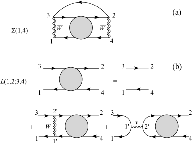
On the basis of this discussion we propose to calculate the Green’s function appearing in Eq. (10) using the self-energy in Fig. 2 (a) where the two-particle correlation function

$$L(1,2;3,4)\equiv-G_{2}(1,2;3,4)+G(1;3)G(2;4)$$

is given in Fig. 2 (b) and is evaluated using excited qp Green’s functions. The latter are calculated by performing numerical simulations of the dynamics of the system in the presence of the pump field. This can be done fully ab initio using, e.g., the Yambo code MHGV.2009 which implements a one-time Kadanoff-Baym evolution for the electronic populations.lsv.1986 ; bonitz.book ; anttibook ; BSH.1999 ; HB.1996 ; M.2013 Previous studies on bulk silicon sm.2015 ; sm2.2015 ; SDCMCM.2016 have shown that the polarization dies off a few femtoseconds after the pump pulse due to inelastic scattering and that the pumped electrons reach a Fermi-Dirac distribution $f(\epsilon)=1/(e^{\beta(\epsilon-\mu)}+1)$ with band-dependent temperature $1/\beta$ and chemical potential $\mu$. Electron-hole recombination and hence relaxation toward the ground state does instead occur on a picosecond time-scale. Thus, the solid is well described by an admixture of stationary excited states on the (femtosecond) time-scale of the probe pulse.PSMS.2015 It is the purpose of this Section to develop a first-principles approach to nonequilibrium PE in such regime.

V.1 Excited two-particle correlation function

As the screened interaction $W$ in Fig. 2 (a) is static, the vertices $(1,3)$ and $(2,4)$ have the same time argument. It is therefore sufficient to evaluate

$$L_{\begin{subarray}{c}{\mathbf{x}}_{1}{\mathbf{x}}_{3}\\ {\mathbf{x}}_{2}{\mathbf{x}}_{4}\end{subarray}}(z,z^{\prime})\equiv L({\mathbf{x}}_{1}z,{\mathbf{x}}_{2}z^{\prime};{\mathbf{x}}_{3}z,{\mathbf{x}}_{4}z^{\prime}),$$

where ${\mathbf{x}}=({\mathbf{r}}\sigma)$ is a collective index for the position and spin coordinate whereas $z$ is a contour time. The Green’s function lines in Fig. 2 (b) describe qp propagators in some admixture of stationary excited states

$$g_{{\mathbf{x}}_{1}{\mathbf{x}}_{4}}(z,z^{\prime})=\sum_{j}\varphi_{i}({\mathbf{x}}_{1})\varphi_{j}^{\ast}({\mathbf{x}}_{4})g_{j}(z,z^{\prime}),$$ (14)

where $\varphi_{j}$ is the qp wavefunction and $j$ is a collective index for the band, spin and momentum. Expanding $L$ according to

$$L_{\begin{subarray}{c}{\mathbf{x}}_{1}{\mathbf{x}}_{3}\\ {\mathbf{x}}_{2}{\mathbf{x}}_{4}\end{subarray}}(z,z^{\prime})=\sum_{\begin{subarray}{c}ij\\ mn\end{subarray}}L_{\begin{subarray}{c}ij\\ mn\end{subarray}}(z,z^{\prime})\varphi_{i}({\mathbf{x}}_{1})\varphi_{j}^{\ast}({\mathbf{x}}_{3})\varphi_{m}({\mathbf{x}}_{2})\varphi_{n}^{\ast}({\mathbf{x}}_{4}),$$ (15)

the BSE of Fig. 2(b) takes the form

$$L_{\vbox{\Let@\restore@math@cr\default@tag\halign{\hfil$\m@th\scriptstyle#$&$\m@th\scriptstyle{}#$\cr&ij\\ &mn\crcr}}}(z,z^{\prime})=\delta_{in}\delta_{jm}\,g_{i}(z,z^{\prime})g_{j}(z^{\prime},z)+i\sum_{pq}\int d\bar{z}$$ (18)

$$\times g_{i}(z,\bar{z})g_{j}(\bar{z},z)K_{\vbox{\Let@\restore@math@cr\default@tag\halign{\hfil$\m@th\scriptstyle#$&$\m@th\scriptstyle{}#$\cr&ij\\ &qp\crcr}}}L_{\vbox{\Let@\restore@math@cr\default@tag\halign{\hfil$\m@th\scriptstyle#$&$\m@th\scriptstyle{}#$\cr&pq\\ &mn\crcr}}}(\bar{z},z^{\prime}),$$ (23)

where $K_{\vbox{\Let@\restore@math@cr\default@tag\halign{\hfil$\m@th\scriptstyle#$&$\m@th\scriptstyle{}#$\cr&ij\\ &qp\crcr}}}\equiv W_{iqjp}-v_{iqpj}$. Here the four-index statically screened interaction is defined according to

$$W_{ijmn}=\!\!\int\!\!d{\mathbf{x}}_{1}d{\mathbf{x}}_{2}\,\varphi_{i}^{\ast}({\mathbf{x}}_{1})\varphi_{j}^{\ast}({\mathbf{x}}_{2})\varphi_{m}({\mathbf{x}}_{2})\varphi_{n}({\mathbf{x}}_{1})W({\mathbf{x}}_{1},{\mathbf{x}}_{2}).$$ (24)

The definition of the four-index bare interaction is analogous and is obtained by replacing $W$ with $v$ in Eq. (24).

To take advantage of the conservation of momentum we write every label $i,j,\ldots$ in terms of a collective greek index that specifies band and spin, and a latin bold index that specifies the value of the momentum, e.g., $i=\alpha{\mathbf{k}}$, $j=\beta{\mathbf{p}}$, etc. Since we are describing electrons bound to the solid all momenta have vanishing component perpendicular to the surface. Momentum conservation implies that the sum of the momenta of the indices $(i,q)$ in $K_{\vbox{\Let@\restore@math@cr\default@tag\halign{\hfil$\m@th\scriptstyle#$&$\m@th\scriptstyle{}#$\cr&ij\\ &qp\crcr}}}$ is the same as the sum of the momenta of the indices $(j,p)$. Therefore

$$K_{\vbox{\Let@\restore@math@cr\default@tag\halign{\hfil$\m@th\scriptstyle#$&$\m@th\scriptstyle{}#$\cr&\mu{\mathbf{k}}+{\mathbf{q}},\nu{\mathbf{k}}\\ &\alpha{\mathbf{k}}''+{\mathbf{q}}-{\mathbf{q}}'',\beta{\mathbf{k}}''+{\mathbf{q}}\crcr}}}=\delta_{{\mathbf{q}}{\mathbf{q}}^{\prime\prime}}K^{{\mathbf{q}}}_{\vbox{\Let@\restore@math@cr\default@tag\halign{\hfil$\m@th\scriptstyle#$&$\m@th\scriptstyle{}#$\cr&\mu\nu{\mathbf{k}}\\ &\alpha\beta{\mathbf{k}}''\crcr}}},$$ (25)

which implicitly defines the tensor on the right hand side. For a tensor $K$ with the property in Eq. (25) the solution of Eq. (23) is a tensor $L$ with the same property. Thus the BSE reduces to

$$L^{{\mathbf{q}}}_{\vbox{\Let@\restore@math@cr\default@tag\halign{\hfil$\m@th\scriptstyle#$&$\m@th\scriptstyle{}#$\cr&\mu\nu{\mathbf{k}}\\ &\rho\sigma{\mathbf{k}}^{\prime}\crcr}}}(z,z^{\prime})=\delta_{\mu\sigma}\delta_{\nu\rho}\delta_{{\mathbf{k}}{\mathbf{k}}^{\prime}}g_{\mu{\mathbf{k}}+{\mathbf{q}}}(z,z^{\prime})g_{\nu{\mathbf{k}}}(z^{\prime},z)$$ (28)

$$+i\sum_{\alpha\beta{\mathbf{k}}^{\prime\prime}}\int\!d\bar{z}\,g_{\mu{\mathbf{k}}+{\mathbf{q}}}(z,\bar{z})g_{\nu{\mathbf{k}}}(\bar{z},z)K^{{\mathbf{q}}}_{\vbox{\Let@\restore@math@cr\default@tag\halign{\hfil$\m@th\scriptstyle#$&$\m@th\scriptstyle{}#$\cr&\mu\nu{\mathbf{k}}\\ &\alpha\beta{\mathbf{k}}^{\prime\prime}\crcr}}}L^{{\mathbf{q}}}_{\vbox{\Let@\restore@math@cr\default@tag\halign{\hfil$\m@th\scriptstyle#$&$\m@th\scriptstyle{}#$\cr&\beta\alpha{\mathbf{k}}^{\prime\prime}\\ &\rho\sigma{\mathbf{k}}^{\prime}\crcr}}}(\bar{z},z^{\prime}).\quad$$ (33)

Introducing the superindices $I=(\mu\nu{\mathbf{k}})$, $J=(\sigma\rho{\mathbf{k}}^{\prime})$ etc. and using the convention that lower superindices have swapped band-spin indices, e.g. $A_{\begin{subarray}{c}I\\ J\end{subarray}}=A_{\begin{subarray}{c}\mu\nu{\mathbf{k}}\\ \rho\sigma{\mathbf{k}}^{\prime}\end{subarray}}$, we can rewrite Eq. (33) in the following compact form

$$L^{{\mathbf{q}}}_{\begin{subarray}{c}I\\ J\end{subarray}}(z,z^{\prime})=\delta_{\begin{subarray}{c}I\\ J\end{subarray}}\ell^{{\mathbf{q}}}_{I}(z,z^{\prime})+i\sum_{M}\int\!d\bar{z}\,\ell^{{\mathbf{q}}}_{I}(z,\bar{z})K^{{\mathbf{q}}}_{\begin{subarray}{c}I\\ M\end{subarray}}L^{{\mathbf{q}}}_{\begin{subarray}{c}M\\ J\end{subarray}}(\bar{z},z^{\prime}),$$ (34)

where $\delta_{\begin{subarray}{c}I\\ J\end{subarray}}=\delta_{\begin{subarray}{c}\mu\nu{\mathbf{k}}\\ \rho\sigma{\mathbf{k}}^{\prime}\end{subarray}}\equiv\delta_{\mu\sigma}\delta_{\nu\rho}\delta_{{\mathbf{k}}{\mathbf{k}}^{\prime}}$ and

$$\ell^{{\mathbf{q}}}_{I}(z,z^{\prime})=\ell^{{\mathbf{q}}}_{\mu\nu{\mathbf{k}}}(z,z^{\prime})\equiv g_{\mu{\mathbf{k}}+{\mathbf{q}}}(z,z^{\prime})g_{\nu{\mathbf{k}}}(z^{\prime},z)$$

is the free eh propagator. The Green’s function $g$ is an excited qp Green’s function and therefore the lesser and greater components are given by

$$g^{<}_{\mu{\mathbf{k}}}(\omega)=2\pi if_{\mu{\mathbf{k}}}\delta(\omega-\epsilon_{\mu{\mathbf{k}}}),$$ (35a)

$$g^{>}_{\mu{\mathbf{k}}}(\omega)=-2\pi i\bar{f}_{\mu{\mathbf{k}}}\delta(\omega-\epsilon_{\mu{\mathbf{k}}}),$$ (35b)

where $f_{\mu{\mathbf{k}}}$ is the qp occupation of level $\mu{\mathbf{k}}$ with energy $\epsilon_{\mu{\mathbf{k}}}$ whereas $\bar{f}_{\mu{\mathbf{k}}}=1-f_{\mu{\mathbf{k}}}$. Since the solid is in an admixture of excited states the occupations do not follow a thermal distribution. It is straightforward to extract the lesser/greater component of $\ell^{{\mathbf{q}}}$:

$$\ell^{{\mathbf{q}},>}_{\mu\nu{\mathbf{k}}}(\omega) = \int\frac{d\omega^{\prime}}{2\pi}g^{>}_{\mu{\mathbf{k}}+{\mathbf{q}}}(\omega+\omega^{\prime})g^{<}_{\nu{\mathbf{k}}}(\omega^{\prime})$$ (36)

$$= 2\pi\bar{f}_{\mu{\mathbf{k}}+{\mathbf{q}}}f_{\nu{\mathbf{k}}}\delta(\omega-\epsilon_{\mu{\mathbf{k}}+{\mathbf{q}}}+\epsilon_{\nu{\mathbf{k}}}),\quad$$

and similarly

$$\ell^{{\mathbf{q}},<}_{\mu\nu{\mathbf{k}}}(\omega)=2\pi f_{\mu{\mathbf{k}}+{\mathbf{q}}}\bar{f}_{\nu{\mathbf{k}}}\delta(\omega-\epsilon_{\mu{\mathbf{k}}+{\mathbf{q}}}+\epsilon_{\nu{\mathbf{k}}}).$$ (37)

Therefore

$$\ell^{{\mathbf{q}},\rm R/A}_{\mu\nu{\mathbf{k}}}(\omega) = i\int\frac{d\omega^{\prime}}{2\pi}\frac{\ell^{{\mathbf{q}},>}_{\mu\nu{\mathbf{k}}}(\omega^{\prime})-\ell^{{\mathbf{q}},<}_{\mu\nu{\mathbf{k}}}(\omega^{\prime})}{\omega-\omega^{\prime}\pm i\eta}$$ (38)

$$= i\frac{f_{\nu{\mathbf{k}}}-f_{\mu{\mathbf{k}}+{\mathbf{q}}}}{\omega-\epsilon_{\mu{\mathbf{k}}+{\mathbf{q}}}+\epsilon_{\nu{\mathbf{k}}}\pm i\eta}.$$

Again to keep the notation as light as possible we define

$$f_{I}^{{\mathbf{q}}}=f^{{\mathbf{q}}}_{\mu\nu{\mathbf{k}}}\equiv f_{\nu{\mathbf{k}}}-f_{\mu{\mathbf{k}}+{\mathbf{q}}},$$ (39)

and

$$\omega^{{\mathbf{q}}}_{I}=\omega^{{\mathbf{q}}}_{\mu\nu{\mathbf{k}}}\equiv\epsilon_{\mu{\mathbf{k}}+{\mathbf{q}}}-\epsilon_{\nu{\mathbf{k}}},$$

so that Eq. (38) takes the following compact form

$$\ell^{{\mathbf{q}},\rm R/A}_{I}=i\frac{f_{I}^{{\mathbf{q}}}}{\omega-\omega^{{\mathbf{q}}}_{I}\pm i\eta}.$$ (40)

We now proceed to the calculation of the various Keldysh components of $L$.

V.1.1 Retarded component

Extracting the retarded component of Eq. (34), Fourier transforming and using Eq. (40) we get

$$(\omega-\omega^{{\mathbf{q}}}_{I})L^{{\mathbf{q}},\rm R}_{\begin{subarray}{c}I\\ J\end{subarray}}(\omega)=if_{I}^{{\mathbf{q}}}\delta_{\begin{subarray}{c}I\\ J\end{subarray}}-f_{I}^{{\mathbf{q}}}\sum_{M}K^{{\mathbf{q}}}_{\begin{subarray}{c}I\\ M\end{subarray}}L^{{\mathbf{q}},\rm R}_{\begin{subarray}{c}M\\ J\end{subarray}}(\omega).$$ (41)

Since $f_{I}^{{\mathbf{q}}}=0$ implies $L^{{\mathbf{q}},\rm R}_{\begin{subarray}{c}I\\ J\end{subarray}}=0$ we can solve Eq. (41) in the subspace $\mbox{$\mathcal{S}$}^{{\mathbf{q}}}$ of superindices $I$ such that $f_{I}^{{\mathbf{q}}}\neq 0$, and restrict the sum over $M$ to this subspace. Notice that if $I\in\mbox{$\mathcal{S}$}^{{\mathbf{q}}}$ and $J\notin\mbox{$\mathcal{S}$}^{{\mathbf{q}}}$ then $\delta_{\begin{subarray}{c}I\\ J\end{subarray}}=0$ and therefore Eq. (41) becomes a homogeneous system of equations. Consequently, $L^{{\mathbf{q}},\rm R}_{\begin{subarray}{c}I\\ J\end{subarray}}$ is nonvanishing only for $I,J\in\mbox{$\mathcal{S}$}^{{\mathbf{q}}}$. Let us split the superindices into two classes, one class with $f_{I}^{{\mathbf{q}}}>0$ and the other class with $f_{I}^{{\mathbf{q}}}<0$. We order all vectors and matrices in such a way that the first entries correspond to superindices in the first class. Defining the matrices $\tilde{L}^{{\mathbf{q}}}$ and $\tilde{K}^{{\mathbf{q}}}$ according to SRFHB.2011

$$L^{{\mathbf{q}},\rm R}_{\begin{subarray}{c}I\\ J\end{subarray}}\equiv\sqrt{|f_{I}^{{\mathbf{q}}}|}\,\tilde{L}^{{\mathbf{q}}}_{\begin{subarray}{c}I\\ J\end{subarray}}\sqrt{|f_{J}^{{\mathbf{q}}}|}\quad;\quad\tilde{K}^{{\mathbf{q}}}_{\begin{subarray}{c}I\\ J\end{subarray}}\equiv\sqrt{|f_{I}^{{\mathbf{q}}}|}\,K^{{\mathbf{q}}}_{\begin{subarray}{c}I\\ J\end{subarray}}\sqrt{|f_{J}^{{\mathbf{q}}}|},$$ (42)

we can rewrite Eq. (41) as follows

$$\left[(\omega-\omega^{{\mathbf{q}}})\sigma_{z}^{{\mathbf{q}}}+\tilde{K}^{{\mathbf{q}}}\right]\tilde{L}^{{\mathbf{q}}}=i\mathbbm{1},$$ (43)

where $\mathbbm{1}$ is the identity matrix, $\omega^{{\mathbf{q}}}$ is the diagonal matrix with entries $\omega^{{\mathbf{q}}}_{I}$ and

$$(\sigma_{z}^{{\mathbf{q}}})_{\begin{subarray}{c}I\\ J\end{subarray}}={\rm sign}(f^{{\mathbf{q}}}_{I})\delta_{\begin{subarray}{c}I\\ J\end{subarray}}\;.$$

Since $\tilde{K}^{{\mathbf{q}}}$ is hermitian we see from Eq. (43) that $\tilde{L}^{{\mathbf{q}}}$ is anti-hermitian, i.e., $\tilde{L}^{{\mathbf{q}}}_{\begin{subarray}{c}I\\ J\end{subarray}}=-\tilde{L}^{{\mathbf{q}}\ast}_{\begin{subarray}{c}J\\ I\end{subarray}}$, as it should. Let us denote by $\Omega^{\lambda{\mathbf{q}}}$ the values of $\omega$ for which the matrix in the square brackets of Eq. (43) is singular and by $\tilde{Y}^{\lambda{\mathbf{q}}}$ the vector belonging to the null space of the singular matrix:

$$(\sigma_{z}^{{\mathbf{q}}}\omega^{{\mathbf{q}}}-\tilde{K}^{{\mathbf{q}}})\tilde{Y}^{\lambda{\mathbf{q}}}=\Omega^{\lambda{\mathbf{q}}}\sigma_{z}^{{\mathbf{q}}}\tilde{Y}^{\lambda{\mathbf{q}}}.$$ (44)

For systems in equilibrium $\omega^{{\mathbf{q}}}_{I}\lessgtr 0$ implies that $f^{{\mathbf{q}}}_{I}\gtrless 0$. This property guarantees that the $\Omega^{\lambda{\mathbf{q}}}$’s are all real and can be arranged in pairs with entries of opposite sign. The reality of the $\Omega^{\lambda{\mathbf{q}}}$’s is no longer guaranteed in stationary excited states (or in admixtures of them). However, if the pump is weak, as it is the case of 2PPE experiments,SBN.2004 ; Weinelt-book ; UG.2007 then the qp occupations differ from their equilibrium values by a small amount and the $\Omega^{\lambda{\mathbf{q}}}$’s continue to be real (although they cannot be arranged in pairs any longer). Under the assumption of reality we can normalize the $\tilde{Y}$ vectors according to

$$\tilde{Y}^{\lambda{\mathbf{q}}\ast}_{I}(\sigma_{z}^{{\mathbf{q}}})_{\begin{subarray}{c}I\\ J\end{subarray}}\tilde{Y}^{\lambda^{\prime}{\mathbf{q}}}_{J}=[\tilde{Y}^{\lambda{\mathbf{q}}}]^{{\dagger}}\sigma_{z}^{{\mathbf{q}}}\tilde{Y}^{\lambda^{\prime}{\mathbf{q}}}=s_{\lambda}\delta_{\lambda\lambda^{\prime}},$$ (45)

where $s_{\lambda}$ can be either $1$ or $-1$. From Eq. (44) and from the normalization condition in Eq. (45) it is easy to show that the solution of Eq. (41) with $I,J\in\mbox{$\mathcal{S}$}^{{\mathbf{q}}}$ can be written as

$$L^{{\mathbf{q}},\rm R}_{\begin{subarray}{c}I\\ J\end{subarray}}(\omega)=i\sum_{\lambda}Y^{\lambda{\mathbf{q}}}_{I}\frac{s_{\lambda}}{\omega-\Omega^{\lambda{\mathbf{q}}}+i\eta}Y^{\lambda{\mathbf{q}}\ast}_{J},$$ (46)

where $Y^{\lambda{\mathbf{q}}}_{I}\equiv\sqrt{|f_{I}^{{\mathbf{q}}}|}\;\sum_{\lambda}\tilde{Y}^{\lambda{\mathbf{q}}}_{I}$. The advanced component can be obtained similarly and differs from Eq. (46) only for the sign of the infinitesimal imaginary part of the denominator. Notice that the matrices $L^{{\mathbf{q}},\rm R/A}$ are manifestly anti-hermitian for real $\omega\pm i\eta$, as it should. It is also easy to verify that in the noninteracting case Eq. (46) reduces to $\delta_{\begin{subarray}{c}I\\ J\end{subarray}}\ell^{{\mathbf{q}},\rm R/A}_{I}$ [see Eq. (40)].

V.1.2 Lesser and Greater component

Let us define the diagonal matrix $\ell_{\begin{subarray}{c}I\\ J\end{subarray}}=\delta_{\begin{subarray}{c}I\\ J\end{subarray}}\ell_{I}$. Extracting the greater/lesser component of Eq. (34) and Fourier transforming one finds (omitting the dependence on frequency)

$$\left[\mathbbm{1}-i\ell^{{\mathbf{q}},\rm R}K^{{\mathbf{q}}}\right]L^{{\mathbf{q}},\lessgtr}=\ell^{{\mathbf{q}},\lessgtr}\left[\mathbbm{1}+iK^{{\mathbf{q}}}L^{{\mathbf{q}},\rm A}\right].$$ (47)

We emphasize that this is an equation in the full space of superindices, i.e., matrix multiplication involves also superindices not belonging to $\mbox{$\mathcal{S}$}^{{\mathbf{q}}}$. With the help of Eq. (41) we can solve for $L^{{\mathbf{q}},\lessgtr}$ and find

$$L^{{\mathbf{q}},\lessgtr}=(\mathbbm{1}+iL^{{\mathbf{q}},\rm R}K^{{\mathbf{q}}})\ell^{{\mathbf{q}},\lessgtr}(\mathbbm{1}+iK^{{\mathbf{q}}}L^{{\mathbf{q}},\rm A}).$$

At difference with the retarded/advanced components, the lesser/greater components are nonvanishing also for indices $I,J\notin\mbox{$\mathcal{S}$}^{{\mathbf{q}}}$. For instance, the lesser two-particle correlator is given by

$$L^{{\mathbf{q}},<}_{\begin{subarray}{c}I\\ J\end{subarray}}\!\! = \!\!\delta_{\begin{subarray}{c}I\\ J\end{subarray}}\ell^{{\mathbf{q}},<}_{I},\quad\quad\quad\quad\quad\quad\quad\quad\quad\quad\quad\quad\;\;\,I,J\notin\mbox{$\mathcal{S}$}^{{\mathbf{q}}}$$

$$L^{{\mathbf{q}},<}_{\begin{subarray}{c}I\\ J\end{subarray}}\!\! = \!\!i\ell^{{\mathbf{q}},<}_{I}(K^{{\mathbf{q}}}L^{{\mathbf{q}},\rm A})_{\begin{subarray}{c}I\\ J\end{subarray}},\quad\quad\quad\quad\quad\quad\,I\notin\mbox{$\mathcal{S}$}^{{\mathbf{q}}},J\in\mbox{$\mathcal{S}$}^{{\mathbf{q}}}$$

$$L^{{\mathbf{q}},<}_{\begin{subarray}{c}I\\ J\end{subarray}}\!\! = \!\!i(L^{{\mathbf{q}},\rm R}K^{{\mathbf{q}}})_{\begin{subarray}{c}I\\ J\end{subarray}}\ell^{{\mathbf{q}},<}_{J},\quad\quad\quad\quad\quad\quad\,I\in\mbox{$\mathcal{S}$}^{{\mathbf{q}}},J\notin\mbox{$\mathcal{S}$}^{{\mathbf{q}}}$$

$$L^{{\mathbf{q}},<}_{\begin{subarray}{c}I\\ J\end{subarray}}\!\! = \!\!-\sum_{M\notin\mbox{$\mathcal{S}$}^{{\mathbf{q}}}}(L^{{\mathbf{q}},\rm R}K^{{\mathbf{q}}})_{\begin{subarray}{c}I\\ M\end{subarray}}\ell^{{\mathbf{q}},<}_{M}(K^{{\mathbf{q}}}L^{{\mathbf{q}},\rm A})_{\begin{subarray}{c}M\\ J\end{subarray}}$$

$$+ \!\!2\eta\sum_{\alpha\beta{\mathbf{p}}\in\mbox{$\mathcal{S}$}^{{\mathbf{q}}}}L^{{\mathbf{q}},\rm R}_{\begin{subarray}{c}I\\ \beta\alpha{\mathbf{p}}\end{subarray}}\frac{f_{\alpha{\mathbf{p}}+{\mathbf{q}}}\bar{f}_{\beta{\mathbf{p}}}}{(f^{{\mathbf{q}}}_{\alpha\beta{\mathbf{p}}})^{2}}L^{{\mathbf{q}},\rm A}_{\begin{subarray}{c}\alpha\beta{\mathbf{p}}\\ J\end{subarray}},\quad\;\;\;\,I,J\in\mbox{$\mathcal{S}$}^{{\mathbf{q}}}$$

where in the second term of the last equality we used

$$\ell^{{\mathbf{q}},<}_{\alpha\beta{\mathbf{p}}}=2\eta\;\ell^{{\mathbf{q}},\rm R}_{\alpha\beta{\mathbf{p}}}\;\frac{f_{\alpha{\mathbf{p}}+{\mathbf{q}}}\bar{f}_{\beta{\mathbf{p}}}}{(f^{{\mathbf{q}}}_{\alpha\beta{\mathbf{p}}})^{2}}\;\ell^{{\mathbf{q}},\rm A}_{\alpha\beta{\mathbf{p}}},$$ (49)

as it follows from the explicit expressions in Eqs. (37) and (40) and from the identity $\eta/(\omega^{2}+\eta^{2})=\pi\delta(\omega)$.

Although every term can be explicitly calculated we here make an approximation that is well justified in the physical regime we are working, i.e., the regime of weak pumps. In this regime the qp occupations $f_{\mu{\mathbf{k}}}$ are either close to zero or close to 1. If $I=(\mu\nu{\mathbf{k}})\notin\mbox{$\mathcal{S}$}^{{\mathbf{q}}}$ then [see Eq. (39)] $f^{{\mathbf{q}}}_{I}=f_{\nu{\mathbf{k}}}-f_{\mu{\mathbf{k}}+{\mathbf{q}}}=0$ which implies that both $f_{\nu{\mathbf{k}}}$ and $f_{\mu{\mathbf{k}}+{\mathbf{q}}}$ are either close to zero or close to 1 and hence that both products $f_{\nu{\mathbf{k}}}\bar{f}_{\mu{\mathbf{k}}+{\mathbf{q}}}$ and $\bar{f}_{\nu{\mathbf{k}}}f_{\mu{\mathbf{k}}+{\mathbf{q}}}$ are close to zero. Taking into account Eqs. (36) and (37) we then see that $\ell^{{\mathbf{q}},\lessgtr}_{I}$ is small for $I\notin\mbox{$\mathcal{S}$}^{{\mathbf{q}}}$. Approximating

$$\ell^{{\mathbf{q}},\lessgtr}_{I}\simeq 0\quad\quad{\rm for}\;I\notin\mbox{$\mathcal{S}$}^{{\mathbf{q}}},$$

we can write for all $I$ and $J$

$$L^{{\mathbf{q}},<}_{\begin{subarray}{c}I\\ J\end{subarray}}(\omega)=-2\eta\sum_{\alpha\beta{\mathbf{p}}\in\mbox{$\mathcal{S}$}^{{\mathbf{q}}}}L^{{\mathbf{q}},\rm R}_{\begin{subarray}{c}I\\ \beta\alpha{\mathbf{p}}\end{subarray}}(\omega)\frac{f_{\alpha{\mathbf{p}}+{\mathbf{q}}}\bar{f}_{\beta{\mathbf{p}}}}{(f^{{\mathbf{q}}}_{\alpha\beta{\mathbf{p}}})^{2}}L^{{\mathbf{q}},\rm A}_{\begin{subarray}{c}\alpha\beta{\mathbf{p}}\\ J\end{subarray}}(\omega).$$ (50)

We now insert in Eq. (50) the spectral decomposition for the retarded/advanced two-particle correlator, see Eq. (46). The resulting double sum over $\lambda,\lambda^{\prime}$ can be split into a sum over $\lambda=\lambda^{\prime}$ and a sum over $\lambda\neq\lambda^{\prime}$. In the limit $\eta\to 0$ the latter is finite whereas the former yields a sum of $\delta$-functions. We can then restrict the sum to $\lambda=\lambda^{\prime}$ and get

$$L^{{\mathbf{q}},<}_{\begin{subarray}{c}I\\ J\end{subarray}}(\omega)=2\pi\,\sum_{\lambda}F^{\lambda{\mathbf{q}}}\,Y^{\lambda{\mathbf{q}}}_{I}\,\delta(\omega-\Omega^{\lambda{\mathbf{q}}})\,Y^{\lambda{\mathbf{q}}\ast}_{J}\;\;,$$ (51)

where we have defined

$$F^{\lambda{\mathbf{q}}}\equiv\sum_{\alpha\beta{\mathbf{p}}\in\mbox{$\mathcal{S}$}^{{\mathbf{q}}}}Y^{\lambda{\mathbf{q}}\ast}_{\alpha\beta{\mathbf{p}}}\,\frac{f_{\alpha{\mathbf{p}}+{\mathbf{q}}}\bar{f}_{\beta{\mathbf{p}}}}{(f^{{\mathbf{q}}}_{\alpha\beta{\mathbf{p}}})^{2}}\,Y^{\lambda{\mathbf{q}}}_{\alpha\beta{\mathbf{p}}},$$

and introduced the convention $Y^{\lambda{\mathbf{q}}}_{I}=0$ for $I\notin\mbox{$\mathcal{S}$}^{{\mathbf{q}}}$. A similar expression can be derived for the greater component

$$L^{{\mathbf{q}},>}_{\begin{subarray}{c}I\\ J\end{subarray}}(\omega)=2\pi\,\sum_{\lambda}\bar{F}^{\lambda{\mathbf{q}}}\,Y^{\lambda{\mathbf{q}}}_{I}\,\delta(\omega-\Omega^{\lambda{\mathbf{q}}})\,Y^{\lambda{\mathbf{q}}\ast}_{J}\;\;,$$ (52)

where we have defined

$$\bar{F}^{\lambda{\mathbf{q}}}\equiv\sum_{\alpha\beta{\mathbf{p}}\in\mbox{$\mathcal{S}$}^{{\mathbf{q}}}}Y^{\lambda{\mathbf{q}}\ast}_{\alpha\beta{\mathbf{p}}}\,\frac{\bar{f}_{\alpha{\mathbf{p}}+{\mathbf{q}}}f_{\beta{\mathbf{p}}}}{(f^{{\mathbf{q}}}_{\alpha\beta{\mathbf{p}}})^{2}}\,Y^{\lambda{\mathbf{q}}}_{\alpha\beta{\mathbf{p}}}.$$

We have verified that Eqs. (51) and (52) reduce to $\ell^{{\mathbf{q}},\lessgtr}(\omega)$ in the noninteracting case and that in equilibrium we recover the fluctuation dissipation theorem.

V.2 Excited self-energy and Green’s function

Let us evaluate $\Sigma_{{\mathbf{x}}_{1}{\mathbf{x}}_{4}}(z,z^{\prime})$ in Fig. 2 (a). Expanding the self-energy analogously to the Green’s function [see Eq. (14)], i.e.,

$$\Sigma_{{\mathbf{x}}_{1}{\mathbf{x}}_{4}}(z,z^{\prime})=\sum_{pq}\varphi_{p}({\mathbf{x}}_{1})\varphi_{q}^{\ast}({\mathbf{x}}_{4})\Sigma_{pq}(z,z^{\prime}),$$

and taking into account the expansion of $L$ in Eq. (15) as well as the definition of the four-index screened interaction in Eq. (24), it is a matter of simple algebra to find

$$\Sigma_{pq}(z,z^{\prime})=-i^{2}\sum_{ijmnk}g_{k}(z,z^{\prime})\,W_{\begin{subarray}{c}pk\\ ji\end{subarray}}\,L_{\begin{subarray}{c}ij\\ mn\end{subarray}}(z,z^{\prime})W_{\begin{subarray}{c}nm\\ kq\end{subarray}},$$

where $W_{\begin{subarray}{c}pk\\ ji\end{subarray}}\equiv W_{pjki}$ (in analogy with the definition of the kernel $K$ in Eq. (23)). Extracting the lesser/greater component, Fourier transforming and using Eqs. (35) we find

$$\Sigma_{pq}^{<}(\omega)=i\sum_{ijmnk}f_{k}\,W_{\begin{subarray}{c}pk\\ ji\end{subarray}}\,L_{\begin{subarray}{c}ij\\ mn\end{subarray}}^{<}(\omega-\epsilon_{k})W_{\begin{subarray}{c}nm\\ kq\end{subarray}},$$

$$\Sigma_{pq}^{>}(\omega)=-i\sum_{ijmnk}\bar{f}_{k}\,W_{\begin{subarray}{c}pk\\ ji\end{subarray}}\,L_{\begin{subarray}{c}ij\\ mn\end{subarray}}^{>}(\omega-\epsilon_{k})W_{\begin{subarray}{c}nm\\ kq\end{subarray}}.$$

We make explicit the dependence on the band-spin indices and momenta. Due to momentum conservation $\Sigma_{\mu{\mathbf{p}}\nu{\mathbf{p}}^{\prime}}=\delta_{{\mathbf{p}}{\mathbf{p}}^{\prime}}\Sigma_{\mu\nu{\mathbf{p}}}$. After some algebra the lesser self-energy takes the form

$$\Sigma^{<}_{\mu\nu{\mathbf{p}}}(\omega)=i\!\!\sum_{IJ,\gamma{\mathbf{q}}}\!f_{\gamma{\mathbf{p}}-{\mathbf{q}}}W^{{\mathbf{q}}}_{\vbox{\Let@\restore@math@cr\default@tag\halign{\hfil$\m@th\scriptstyle#$&$\m@th\scriptstyle{}#$\cr&\mu\gamma{\mathbf{p}}-{\mathbf{q}}\\ &I\crcr}}}L^{{\mathbf{q}},<}_{\vbox{\Let@\restore@math@cr\default@tag\halign{\hfil$\m@th\scriptstyle#$&$\m@th\scriptstyle{}#$\cr&I\\ &J\crcr}}}(\omega-\epsilon_{\gamma{\mathbf{p}}-{\mathbf{q}}})W^{{\mathbf{q}}}_{\vbox{\Let@\restore@math@cr\default@tag\halign{\hfil$\m@th\scriptstyle#$&$\m@th\scriptstyle{}#$\cr&J\\ &\gamma\nu{\mathbf{p}}-{\mathbf{q}}\crcr}}}$$ (54)

with a similar expression for the greater self-energy. In Eq. (54) the sum is restricted to $I,J\in\mbox{$\mathcal{S}$}^{{\mathbf{q}}}$ due to the approximation in Eq. (50), according to which $L^{{\mathbf{q}},<}_{\begin{subarray}{c}I\\ J\end{subarray}}$ vanishes if $I$ and/or $J$ do not belong to $\mbox{$\mathcal{S}$}^{{\mathbf{q}}}$. Inserting the expansion in Eq. (51) we get

$$\Sigma^{<}_{\mu\nu{\mathbf{p}}}(\omega)\!\! = \!\!2\pi i\sum_{\lambda}\sum_{IJ,\gamma{\mathbf{q}}}f_{\gamma{\mathbf{p}}-{\mathbf{q}}}F^{\lambda{\mathbf{q}}}W^{{\mathbf{q}}}_{\vbox{\Let@\restore@math@cr\default@tag\halign{\hfil$\m@th\scriptstyle#$&$\m@th\scriptstyle{}#$\cr&\mu\gamma{\mathbf{p}}-{\mathbf{q}}\\ &I\crcr}}}\,Y^{\lambda{\mathbf{q}}}_{I}$$ (57)

$$\times \!\!\delta(\omega-\epsilon_{\gamma{\mathbf{p}}-{\mathbf{q}}}-\Omega^{\lambda{\mathbf{q}}})\,Y^{\lambda{\mathbf{q}}\ast}_{J}W^{{\mathbf{q}}}_{\vbox{\Let@\restore@math@cr\default@tag\halign{\hfil$\m@th\scriptstyle#$&$\m@th\scriptstyle{}#$\cr&J\\ &\gamma\nu{\mathbf{p}}-{\mathbf{q}}\crcr}}}.$$ (60)

Following similar steps the greater self-energy reads

$$\Sigma^{>}_{\mu\nu{\mathbf{p}}}(\omega)\!\! = \!\!-2\pi i\sum_{\lambda}\sum_{IJ,\gamma{\mathbf{q}}}\bar{f}_{\gamma{\mathbf{p}}-{\mathbf{q}}}\bar{F}^{\lambda{\mathbf{q}}}\,W^{{\mathbf{q}}}_{\vbox{\Let@\restore@math@cr\default@tag\halign{\hfil$\m@th\scriptstyle#$&$\m@th\scriptstyle{}#$\cr&\mu\gamma{\mathbf{p}}-{\mathbf{q}}\\ &I\crcr}}}\,Y^{\lambda{\mathbf{q}}}_{I}$$ (63)

$$\times \!\!\delta(\omega-\epsilon_{\gamma{\mathbf{p}}-{\mathbf{q}}}-\Omega^{\lambda{\mathbf{q}}})\,Y^{\lambda{\mathbf{q}}\ast}_{J}W^{{\mathbf{q}}}_{\vbox{\Let@\restore@math@cr\default@tag\halign{\hfil$\m@th\scriptstyle#$&$\m@th\scriptstyle{}#$\cr&J\\ &\gamma\nu{\mathbf{p}}-{\mathbf{q}}\crcr}}},$$ (66)

and hence the retarded/advanced self-energy follows from the Hilbert transform

$$\Sigma^{\rm R/A}_{\mu\nu{\mathbf{p}}}(\omega) = \sum_{\lambda}\sum_{IJ,\gamma{\mathbf{q}}}W^{{\mathbf{q}}}_{\vbox{\Let@\restore@math@cr\default@tag\halign{\hfil$\m@th\scriptstyle#$&$\m@th\scriptstyle{}#$\cr&\mu\gamma{\mathbf{p}}-{\mathbf{q}}\\ &I\crcr}}}\,Y^{\lambda{\mathbf{q}}}_{I}$$ (69)

$$\times \frac{\bar{f}_{\gamma{\mathbf{p}}-{\mathbf{q}}}\bar{F}^{\lambda{\mathbf{q}}}+f_{\gamma{\mathbf{p}}-{\mathbf{q}}}F^{\lambda{\mathbf{q}}}}{\omega-\epsilon_{\gamma{\mathbf{p}}-{\mathbf{q}}}-\Omega^{\lambda{\mathbf{q}}}\pm i\eta}\,Y^{\lambda{\mathbf{q}}\ast}_{J}W^{{\mathbf{q}}}_{\vbox{\Let@\restore@math@cr\default@tag\halign{\hfil$\m@th\scriptstyle#$&$\m@th\scriptstyle{}#$\cr&J\\ &\gamma\nu{\mathbf{p}}-{\mathbf{q}}\crcr}}}.\quad\;\;$$ (72)

Equation (72) does not contain any empirical parameter; it provides the nonequilibrium self-energy in terms of quantities that can all be obtained ab initio.

As the self-energy is diagonal in momentum space the dressed Green’s function $G$ is diagonal too. Therefore, it is convenient to manipulate matrices with indices only in the band-spin sector. We define $(\Sigma_{{\mathbf{k}}})_{\alpha\beta}\equiv\Sigma_{\alpha\beta{\mathbf{k}}}$, $(\epsilon_{{\mathbf{k}}})_{\alpha\beta}\equiv\delta_{\alpha\beta}\epsilon_{\alpha{\mathbf{k}}}$, and $(G_{{\mathbf{k}}})_{\alpha\beta}\equiv G_{\alpha\beta{\mathbf{k}}}$. Then, the retarded Green’s function can be calculated from

$$G^{\rm R/A}_{{\mathbf{k}}}(\omega)=\frac{1}{\omega-\epsilon_{{\mathbf{k}}}-\Sigma^{\rm R/A}_{{\mathbf{k}}}(\omega)}.$$ (73)

ExperimentsCRCZGBBKGP.2012 ; SYACFKS.2012 ; NOHFMEAABEC.2014 ; BVLNL.2014 and numerical simulations sm.2015 ; SDCMCM.2016 indicate that the electron occupations in the quasi-stationary excited state follow a Fermi-Dirac distribution with temperatures $T_{\alpha}$ and chemical potentials $\mu_{\alpha}$ depending on the band-spin index $\alpha$. Of course $T_{\alpha}$ and $\mu_{\alpha}$ vary on a picosecond time-scale but they can be considered as constant on the time-scale of the probe pulse. From this evidence we infer that the recombination of electrons with different band-spin index $\alpha$ is severely suppressed and that the lesser Green’s function fulfills the approximate fluctuation-dissipation relation

$$G^{<}_{\alpha\beta{\mathbf{k}}}(\omega)=-\delta_{\alpha\beta}f_{\alpha}(\omega)[G^{\rm R}_{\alpha\alpha{\mathbf{k}}}(\omega)-G^{\rm A}_{\alpha\alpha{\mathbf{k}}}(\omega)],$$ (74)

where $f_{\alpha}(\omega)=1/(e^{(\omega-\mu_{\alpha})/T_{\alpha}}+1)$. The $\alpha$-dependent temperature and chemical potential can be extracted by a best fitting of the electronic populations as obtained from, e.g., the one-time Kadanoff-Baym propagation.sm.2015 Using the Green’s function of Eq. (74) in Eq. (10) the photocurrent follows.

This concludes our first-principle diagrammatic approach to deal with excitonic features in TR-PE spectra. In the next Section we study excitonic features in a minimal model and assess the accuracy of the proposed theory.

VI Application to a Minimal Model

We consider a one-dimensional insulator of length $\mathcal{L}$ with one valence band and one conduction band separated by a direct gap of strength $\Delta$.YLU.2012 Since the formation of excitons is due to the attraction between a valence hole and a conduction electron we discard the Coulomb interaction between electrons in the same band. For simplicity we also discard spin. Thus, the Hamiltonian of the insulator reads

$$\hat{H}_{\rm ins} = \sum_{k}(\epsilon_{vk}\hat{v}^{{\dagger}}_{k}\hat{v}_{k}+\epsilon_{ck}\hat{c}^{{\dagger}}_{k}\hat{c}_{k})-U(0)\frac{N_{v}}{\mbox{$\mathcal{L}$}}\sum_{k}\hat{c}^{{\dagger}}_{k}\hat{c}_{k}$$ (75)

$$+ \frac{1}{\mbox{$\mathcal{L}$}}\sum_{k_{1}k_{2}q}U(q)\,\hat{v}^{{\dagger}}_{k_{1}+q}\hat{c}^{{\dagger}}_{k_{2}-q}\hat{c}_{k_{2}}\hat{v}_{k_{1}},$$

where $\hat{v}_{k}$ ($\hat{c}_{k}$) annihilates an electron of momentum $k$ in the valence (conduction) band and $W(q)\equiv U(q)/\mbox{$\mathcal{L}$}$ is the statically screened interaction. The last term in the first row represents the interaction of a conduction electron with the positive background in the valence band, $N_{v}$ being the number of protons (which is also equal to the number of valence electrons in the ground state). For this model the ground state is obtained by filling all single-particle valence states with one electron. Hence the interaction between the valence background and the conduction electrons vanishes.

VI.1 Analytic treatment for a single bound exciton

The insulator Hamiltonian commutes with the total number of conduction electrons $\hat{N}_{c}=\sum_{k}\hat{c}^{{\dagger}}_{k}\hat{c}_{k}$ and with the total number of valence electrons $\hat{N}_{v}=\sum_{k}\hat{v}^{{\dagger}}_{k}\hat{v}_{k}$. We consider the special case of a stationary excited state of vanishing total momentum with one electron in the conduction band (and hence with one hole in the valence band). Denoting by $|\Psi_{g}\rangle=\prod_{k}\hat{v}^{{\dagger}}_{k}|0\rangle$ the ground state of energy $E_{g}$ we write this excited state as

$$|\Psi\rangle=\sum_{k}Y_{k}\hat{c}^{{\dagger}}_{k}\hat{v}_{k}|\Psi_{g}\rangle=\sum_{k}Y_{k}|\Phi_{k}\rangle,$$ (76)

where we introduced the eh states $|\Phi_{k}\rangle\equiv\hat{c}^{{\dagger}}_{k}\hat{v}_{k}|\Psi_{g}\rangle$. It is a matter of straightforward algebra to show that $\hat{H}_{\rm ins}|\Psi\rangle$ is again a linear combination of the $|\Phi_{k}\rangle$’s. The possible excited state energies $E=E_{g}+\Omega$ are found by solving the eigenvalue problem

$$(\omega_{k-q}-\Omega)Y_{k}=\frac{1}{\mbox{$\mathcal{L}$}}\sum_{q}U(q)Y_{k-q},$$ (77)

with $\omega_{k}\equiv\epsilon_{ck}-\epsilon_{vk}>\Delta=\epsilon_{c0}-\epsilon_{v0}$. For a momentum independent interaction $U(q)=U>0$ the expansion coefficients have the form

$$Y_{k}=\frac{\sqrt{R}}{\omega_{k}-\Omega},$$ (78)

where the positive constant $R$ is fixed by the normalization $\sum_{k}|Y_{k}|^{2}=1$. Equation (77) has a continuum of solutions $\Omega=\Delta-b$ with $b<0$ and one split-off solution $\Omega_{X}=\Delta-b_{X}$ with binding energy $b_{X}>0$. The latter corresponds to a bound eh state or exciton. Notice that for any arbitrary small but finite $U$ the excitonic amplitude $Y_{k}\sim 1/\sqrt{\mbox{$\mathcal{L}$}}$ for $\mbox{$\mathcal{L}$}\to\infty$ whereas $b_{X}$ converges to a finite positive value.

By definition, the lesser Green’s function of the system in the exciton state $|\Psi\rangle=|\Psi_{X}\rangle$ is

$$G_{cc,k}^{<}(t,t^{\prime})\!\! = \!\!i\langle\Psi_{X}|\hat{c}^{{\dagger}}_{kH}(t^{\prime})\hat{c}_{kH}(t)|\Psi_{X}\rangle$$

$$= \!\!i\langle\Psi_{X}|\hat{c}^{{\dagger}}_{k}e^{-i(\hat{H}-E_{g}-\Omega_{X})(t^{\prime}-t)}\hat{c}_{k}|\Psi_{X}\rangle.$$

The only many-body states having a nonvanishing overlap with $\hat{c}_{k}|\Psi_{X}\rangle$ are the states $\hat{v}_{p}|\Psi_{g}\rangle$ which are also eigenstates $\hat{H}_{\rm ins}$ with eigenvalue $E_{g}-\epsilon_{vp}$. Inserting a completeness relation to the right of $\hat{c}^{{\dagger}}_{k}$ and Fourier transforming we find the exact result

$$G_{cc,k}^{<}(\omega)=2\pi i|Y_{k}|^{2}\delta(\omega-\Omega_{X}+\epsilon_{vk}).$$ (79)

In the following we show that our diagrammatic approach yields precisely Eq. (79). Before, however, we observe that substitution of Eq. (79) into Eq. (LABEL:photocurr3) leads to the photocurrent

$$I({\mathbf{k}})=2\pi|Y_{k}a_{0}D_{{\mathbf{k}}}|^{2}\delta(\omega_{0}+\Omega_{X}+\epsilon_{vk}-\epsilon_{f{\mathbf{k}}}),$$ (80)

where, without any loss of generality, we took $\omega_{0}>0$ (in this case $G_{cc,k}^{<}(\epsilon_{f{\mathbf{k}}}+\omega_{0})$ does not contribute). Equation (80) agrees with Eq. (1), as it should.

To calculate the (dressed) excited lesser Green’s function diagrammatically we need an excited qp Green’s function $g$. Here we evaluate $g$ in the HF approximation. The excited noninteracting Green’s function $g^{(0)}$ with one conduction electron and one valence hole in the lowest energy state reads

$$g^{(0),<}_{vv,k}(\omega)=2\pi i\,\bar{\delta}_{k0}\,\delta(\omega-\epsilon_{vk}),$$ (81a)

$$g^{(0),>}_{vv,k}(\omega)=-2\pi i\,\delta_{k0}\,\delta(\omega-\epsilon_{vk}),$$ (81b)

$$g^{(0),<}_{cc,k}(\omega)=2\pi i\,\delta_{k0}\,\delta(\omega-\epsilon_{ck}+U(0)N_{v}/\mbox{$\mathcal{L}$}),$$ (81c)

$$g^{(0),>}_{cc,k}(\omega)=-2\pi i\,\bar{\delta}_{k0}\,\delta(\omega-\epsilon_{ck}+U(0)N_{v}/\mbox{$\mathcal{L}$}),$$ (81d)

and $g^{(0),\lessgtr}_{cv,k}=g^{(0),\lessgtr}_{vc,k}=0$. In Eqs. (81) we defined $\bar{\delta}_{k0}=1-\delta_{k0}$. The HF potential contains only the Hartree part since the interaction preserves the band-spin index and $g^{(0)}$ is diagonal. Using Eqs. (81) one finds

$$V_{{\rm HF},\alpha\alpha k}=\delta_{\alpha c}\frac{U(0)}{\mbox{$\mathcal{L}$}}N_{v}+\mbox{$\mathcal{O}$}(1/\mbox{$\mathcal{L}$}).$$ (82)

Accordingly, the excited HF Green’s function is

$$g^{<}_{vv,k}(\omega)=2\pi i\,\bar{\delta}_{k0}\,\delta(\omega-\epsilon_{vk}),$$ (83a)

$$g^{>}_{vv,k}(\omega)=-2\pi i\,\delta_{k0}\,\delta(\omega-\epsilon_{v0}),$$ (83b)

$$g^{<}_{cc,k}(\omega)=2\pi i\,\delta_{k0}\,\delta(\omega-\epsilon_{c0}),$$ (83c)

$$g^{>}_{cc,k}(\omega)=-2\pi i\,\bar{\delta}_{k0}\,\delta(\omega-\epsilon_{ck}).$$ (83d)

We observe that if we used the HF $g^{<}_{cc,k}$ to evaluate the photocurrent in Eq. (LABEL:photocurr3) we would find

$$I({\mathbf{k}})=2\pi|a_{0}D_{{\mathbf{k}}}|^{2}\delta_{k0}\delta(\omega_{0}+\epsilon_{c0}-\epsilon_{f{\mathbf{k}}}),$$

which coincides with the noninteracting limit of Eq. (80), i.e., $Y_{k}=\delta_{k0}$ and $b_{X}=0$. As expected the HF approximation (and any other qp approximation) does not capture the exciton peak in the energy-resolved and angle-resolved photocurrent.

Figure 3: Self-energy diagrams for the model Hamiltonian of Eq. (75).

For the model Hamiltonian in Eq. (75) the self-energy diagrams of Fig. 2 (a) that contain a polarization insertion vanish. Thus, we only need to evaluate the self-energy diagrams in Fig. 3, with the exception of the first (Hartree) diagram. Since we are interested in $G_{cc}$ and since the self-energy has vanishing $cv$ and $vc$ components we only calculate the $cc$ component. For simplicity we also consider the case of vanishing momentum $k=0$ and a momentum independent interaction $U(q)=U$. We have $\Sigma_{cc,0}(z,z^{\prime})\equiv\Sigma(z,z^{\prime})-\Sigma_{\rm H}(z,z^{\prime})$ where $\Sigma$ is the full series of Fig. 3 and $\Sigma_{\rm H}$ is the first diagram of the series. Introducing the averaged eh propagator

$$\ell_{p}(z,z^{\prime})=\frac{1}{\mbox{$\mathcal{L}$}}\sum_{q}g_{cc,q}(z,z^{\prime})g_{vv,p+q}(z^{\prime},z),$$ (84)

we can write the full series as

$$\Sigma(z,z^{\prime})=-\frac{i}{\mbox{$\mathcal{L}$}}\sum_{p}T_{p}(z,z^{\prime})g_{vv,p}(z,z^{\prime}).$$ (85)

where we have defined the $T$-matrix

$$T_{p}(z,z^{\prime})\equiv U\delta(z,z^{\prime})+iU\int dz_{1}\,\ell_{p}(z,z_{1})T_{p}(z_{1},z^{\prime}).$$ (86)

To calculate the lesser and greater components of $\Sigma$ (which are necessary to calculate $G^{<}_{cc,0}$) we need the lesser and greater components of $T_{p}$. This can be achieved without going through the spectral decomposition of Section V.1 since the system is in a pure (excited) state which is simple enough. The spectral decomposition will be used in the next Section where we consider the system in an admixtures of excited states. Using the Langreth rules in Eq. (86) we get

$$T^{\lessgtr}_{p}(\omega)=i\frac{U^{2}}{|1-iU\ell^{\rm R}_{p}(\omega)|^{2}}\ell^{\lessgtr}_{p}(\omega).$$ (87)

From the definition of the eh propagator in Eq. (84) and using the excited HF Green’s functions in Eqs. (83) we find $\ell^{<}_{p}(\omega)=(2\pi/\mbox{$\mathcal{L}$})\delta_{p0}\,\delta(\omega-\Delta)$. Therefore $T^{<}_{p}(\omega)\propto\delta_{p0}$ and consequently the lesser self-energy

$$\Sigma^{<}(t,t^{\prime})=-\frac{i}{\mbox{$\mathcal{L}$}}T^{<}_{0}(t,t^{\prime})g^{<}_{vv,0}(t,t^{\prime})=0.$$

Thus we only need to evaluate the greater self-energy. From Eq. (85)

$$\Sigma^{>}(\omega) = -\frac{i}{\mbox{$\mathcal{L}$}}\sum_{p}\int\frac{d\omega^{\prime}}{2\pi}T^{>}_{p}(\omega-\omega^{\prime})\mathfrak{g}^{>}_{vv,p}(\omega^{\prime})$$ (88)

$$= -\frac{1}{\mbox{$\mathcal{L}$}}T^{>}_{0}(\omega-\epsilon_{v0}).$$

It is important to emphasize that if we had used a ground state $g$ then also $\Sigma^{>}=0$ since there would be no holes in the valence band and hence $g^{>}_{vv,p}=0$. The calculation of $T^{>}_{0}$ requires the explicit form of $\ell^{>}_{0}$ and $\ell^{\rm R}_{0}$. These follow from Eq. (84)

$$\ell^{>}_{0}(\omega)=\frac{2\pi}{\mbox{$\mathcal{L}$}}\sum_{q}\delta(\omega-\omega_{q})+\mbox{$\mathcal{O}$}(1/\mbox{$\mathcal{L}$}),$$ (89)

and

$$\ell_{0}^{\rm R}(\omega)=\frac{1}{\mbox{$\mathcal{L}$}}\sum_{q}\frac{i}{\omega-\omega_{q}+i\eta}+\mbox{$\mathcal{O}$}(1/\mbox{$\mathcal{L}$}).$$ (90)

Substitution of these results into Eq. (87) yields

$$T^{>}_{0}(\omega)=2iU\frac{y(\omega)}{(1-x(\omega))^{2}+y^{2}(\omega)},$$

where we have defined $x(\omega)\equiv{\rm Re}[iU\ell_{0}^{\rm R}(\omega)]$ and $y(\omega)\equiv{\rm Im}[iU\ell_{0}^{\rm R}(\omega)]=(U/2)\ell^{>}_{0}(\omega)$. The quantity $y(\omega)$ vanishes for $\omega<\Delta$, see Eq. (89). However, this does not imply that $T_{0}^{>}(\omega)$ vanishes in the same region. In fact,

$$\lim_{y\rightarrow 0^{+}}\frac{y}{(1-x)^{2}+y^{2}}=\pi\delta(1-x),$$

and hence $T_{0}^{>}(\omega)$ is nonvanishing for $\omega<\Delta$ if in this frequency region $1-x(\omega)=0$. From Eq. (90) we have

$$1-x(\omega)=1+\frac{U}{\mbox{$\mathcal{L}$}}\sum_{q}\frac{1}{\omega-\omega_{q}}=0.$$

This equation is identical to Eq. (77) after the renaming $\omega=\Omega$. Thus $1-x(\omega)=0$ has a continuum of solutions for $\omega>\Delta$ and one split-off solution at $\omega=\Omega_{X}<\Delta$. Therefore $T^{>}_{0}(\omega)$ can be conveniently rewritten as

$$T^{>}_{0}(\omega) = \frac{2\pi iU}{\left|\partial x(\omega)/\partial\omega\right|_{\omega=\Omega_{X}}}\delta(\omega-\Omega_{X})$$ (91)

$$+ 2iU\,{\rm Reg}\left[\frac{y(\omega)}{(1-x(\omega))^{2}+y^{2}(\omega)}\right],$$

where ${\rm Reg}$ denotes the nonsingular part of the function.

We can now evaluate $\Sigma^{>}$ from Eq. (88) as well as the retarded self-energy

$$\Sigma^{\rm R}_{cc,0}(\omega)=-\frac{i}{\mbox{$\mathcal{L}$}}\int\frac{d\omega^{\prime}}{2\pi}\frac{T^{>}_{0}(\omega^{\prime}-\epsilon_{v0})}{\omega-\omega^{\prime}+i\eta}.$$ (92)

The Hartree part does not contribute to $\Sigma^{>}$ and it is therefore correctly removed in Eq. (92). Using Eq. (91) we find

$$\Sigma^{\rm R}_{cc,0}(\omega)=\frac{R_{X}}{\omega-\Omega_{X}-\epsilon_{v0}+i\eta}+\Sigma_{\rm reg}^{\rm R}(\omega),$$ (93)

where

$$R_{X}=\frac{U/\mbox{$\mathcal{L}$}}{\left|\partial x(\omega)/\partial\omega\right|_{\omega=\Omega_{X}}},$$

is the excitonic residue of the singular part whereas $\Sigma_{\rm reg}^{\rm R}$ is the regular (nonsingular) part. Both $R_{X}$ and $\Sigma_{\rm reg}^{\rm R}$ scale like $1/\mbox{$\mathcal{L}$}$ and are therefore infinitesimally small in the thermodynamic limit. Interestingly, $R_{X}$ is exactly the same constant that appears in the normalized excitonic amplitude of Eq. (78).

From the retarded self-energy the retarded Green’s function follows

$$G^{\rm R}_{cc,0}(\omega)=\frac{1}{\omega-\epsilon_{c0}-\Sigma^{\rm R}_{cc,0}(\omega)}.$$

For $\omega\simeq\epsilon_{X}\equiv\Omega_{X}+\epsilon_{v0}=\epsilon_{c0}-b_{X}$ the self-energy is dominated by the first term in Eq. (93). Thus for frequencies in the neighborhood of $\epsilon_{X}$ we can write

$$G^{\rm R}_{cc,0}(\omega\sim\epsilon_{X}) \simeq \frac{1}{\epsilon_{X}-\epsilon_{c0}-\frac{R_{X}}{\omega-\epsilon_{X}+i\eta}}$$

$$= \frac{R_{X}/b^{2}_{X}}{\omega-\epsilon_{X}+i\eta}+\mbox{$\mathcal{O}$}(1/\mbox{$\mathcal{L}$}),$$

where we took into account that $R_{X}\sim 1/\mbox{$\mathcal{L}$}$. In the same neighborhood the spectral function $A=i[G^{\rm R}_{cc,0}-G^{\rm A}_{cc,0}]$ reads

$$A(\omega\simeq\epsilon_{X})\simeq 2\pi Z_{X}\,\delta(\omega-\epsilon_{X}),$$

where we have defined the excitonic qp weight as

$$Z_{X}\equiv\frac{R_{X}}{b_{X}^{2}}.$$

The physical meaning of $Z_{X}$ is the amount of spectral weight that a bare excited electron transfers to the electron in the bound eh pair. We further observe that $Z_{X}$ is precisely the excitonic amplitude $|Y_{0}|^{2}$, see Eq. (78).

To calculate the excited lesser Green’s function we use Eq. (74), i.e., $G^{<}_{cc,0}(\omega)=if_{c}(\omega)A(\omega)$, where $f_{c}(\omega)$ is the Fermi function for the conduction band. To find the temperature $T_{c}$ and chemical potential $\mu_{c}$ we observe that the occupations of the excited state are $f_{ck}=\delta_{k0}$, see Eq. (83c). Therefore $T_{c}=0$ and $\mu_{c}$ is just above $\epsilon_{c0}$. From the previous analysis we know that the spectral function has a $\delta$-like peak in $\omega=\epsilon_{X}<\epsilon_{c0}$ and it is otherwise smooth and nonvanishing for $\omega>\epsilon_{c0}$. More precisely the self-energy is responsible for moving the noninteracting spectral peaks to the right by an amount $\simeq 1/\mbox{$\mathcal{L}$}$. Therefore only the exciton peak is below $\mu_{c}$ and the excited lesser Green’s function reads

$$G^{<}_{cc,0}(\omega)=2\pi iZ_{X}\delta(\omega-\epsilon_{X}).$$

Since $Z_{X}=|Y_{0}|^{2}$ our diagrammatic approach yields the exact result of Eq. (79).

The analysis of this Section supports the validity of the proposed theoretical framework. In the next Section we consider stationary excited states with a smooth distribution of electrons in the conduction band and investigate the behavior of the exciton peak in different regimes.

VI.2 Numerical results at finite eh density

In this Section we study the PE problem for finite eh densities. From Eq. (75) and the definition in Eq. (25) with $K\to W$ we see that

$$W^{q}_{\vbox{\Let@\restore@math@cr\default@tag\halign{\hfil$\m@th\scriptstyle#$&$\m@th\scriptstyle{}#$\cr&\mu\nu k\\ &\alpha\beta k^{\prime}\crcr}}} = W^{q}_{\vbox{\Let@\restore@math@cr\default@tag\halign{\hfil$\m@th\scriptstyle#$&$\m@th\scriptstyle{}#$\cr&\mu k+q\,\nu k\\ &\alpha k^{\prime}\,\beta k^{\prime}+q\crcr}}}$$

$$= W_{\mu k+q,\alpha k^{\prime},\nu k,,\beta k^{\prime}+q}$$

$$= \delta_{\mu\beta}\delta_{\alpha\nu}[\delta_{\mu c}\delta_{\alpha v}+\delta_{\mu v}\delta_{\alpha c}]U/\mbox{$\mathcal{L}$}.$$ (99)

Inserting this result into Eq. (54) and the analogous for the greater self-energy we obtain

$$\Sigma^{<}_{p}(\omega)\equiv\Sigma^{<}_{cc,p}(\omega)=iU^{2}\sum_{q}f_{vp-q}L^{q,<}(\omega-\epsilon_{vp-q}),$$

$$\Sigma^{>}_{p}(\omega)\equiv\Sigma^{>}_{cc,p}(\omega)=-iU^{2}\sum_{q}\bar{f}_{vp-q}L^{q,>}(\omega-\epsilon_{vp-q}),$$

where we defined

$$L^{q,\lessgtr}(\omega)\equiv\frac{1}{\mbox{$\mathcal{L}$}^{2}}\sum_{p_{1}p_{2}}L^{q,\lessgtr}_{\vbox{\Let@\restore@math@cr\default@tag\halign{\hfil$\m@th\scriptstyle#$&$\m@th\scriptstyle{}#$\cr&cvp_{1}\\ &vcp_{2}\crcr}}}(\omega).$$ (101)

In the calculations we solve Eq. (44) for different interaction strengths $U$ and occupations $f_{\alpha p}$. We consider a valence band with energies in the interval $[-w/2,w/2]$ and dispersion $\epsilon_{vk}=(w/2)\!\cos k$ and a conduction band with energies in the interval $[w/2+\Delta,3w/2+\Delta]$ and dispersion $\epsilon_{ck}=-(w/2)\!\cos k+w+\Delta$; $w>0$ is the bandwidth of both bands. The insulator has a direct gap of strength $\Delta$ at $k=0$. The electron occupations $f_{\alpha k}$ in the excited state are Fermi-Dirac distributions with the same temperature $T$ and different chemical potentials $\mu_{\alpha}$

$$f_{\alpha k}=\frac{1}{e^{(\epsilon_{\alpha k}-\mu_{\alpha})/T}+1},\quad\alpha=v,c\,.$$ (102)

Figure 4: Log-plot of $L^{q,<}$ (in arbitrary units) at $q=0$ according to Eq. (51) (dashed black line) and Eq. (LABEL:Lexact) (solid red line). The inset shows the difference between the two curves.

Figure 5: Left panel: lesser Green’s function $-iG^{<}_{cc,0}(\omega)$ (in arbitrary units) for different densities of the conduction electrons $n_{c}$. Right panel: Dependence of the exciton weight $Z_{X}$ on $n_{c}$.

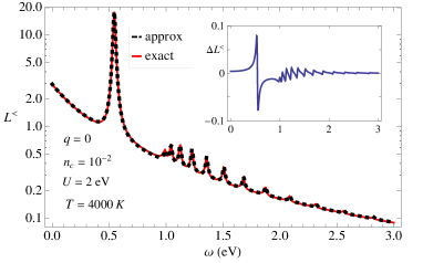
Let us start by assessing the accuracy of the two-particle correlation functions in Eqs. (51) and (52). In Fig. 4 we compare the numerical outcome of $L^{q,<}$ in Eq. (101) obtained by using the approximation of Eq. (51) and the exact result of Eq. (LABEL:Lexact). The system parameters are $\mathcal{L}=80$, $\Delta=w/4=1\,\mathrm{eV}$, $T=4000\,\mathrm{K}$ , $\mu_{v}=2.35\,\mathrm{eV}$, $\mu_{c}=2.65\,\mathrm{eV}$, $U=2\,\mathrm{eV}$, $\eta=w/(4\mathcal{L})$. With these parameters the number of conduction electrons per unit cell is $n_{c}=\frac{1}{\mathcal{L}}\sum_{k}f_{ck}\approx 10^{-2}$ and the solution of Eq. (44) for $q=0$ yields an exciton state with binding energy $b_{X}\approx 0.42\,\mathrm{eV}$. The accuracy of our approximation is excellent in the entire frequency domain. In particular both the exciton structure at $\approx 0.56\,\mathrm{eV}$ and the continuum of eh excitations above $\Delta=1\,\mathrm{eV}$ are well reproduced; the relative error never exceeds 0.5% and reaches its maximum at the exciton energy.

Figure 6: Lesser Green’s function $-iG^{<}_{cc,0}(\omega)$ (in arbitrary units) for different interaction strength $U$ (top panel) and temperatures $T$ (bottom panel).

According to Eq. (LABEL:photocurr3) the energy resolved photocurrent perpendicular to the surface is proportional to $G^{<}_{cc,0}(\epsilon-\omega_{0})$. In Fig. 5 (left panel) we show $G^{<}_{cc,0}(\omega)$ for different carrier densities $n_{c}$. At very low density $n_{c}\lesssim 10^{-4}$ the system is essentially in equilibrium and the photocurrent is vanishingly small (not shown). At density $n_{c}\approx 10^{-3}$ a qp peak at $\omega\approx 3\,\mathrm{eV}$ appears. This corresponds to the removal energy of an excited electron from the bottom of the conduction band. This peak was absent for the singular occupation of the previous Section, i.e., $f_{ck}=\delta_{k0}$, since in that case $T=0$. At $n_{c}\approx 10^{-3}$ the exciton peak at $\epsilon_{X}=\epsilon_{c0}-b_{X}\approx 2.5\,\mathrm{eV}$ is still not visible because the exciton weight $Z_{X}=\int_{-\infty}^{\epsilon_{c0}}\frac{d\omega}{2\pi}A(\omega)$ is still too small. The dependence of $Z_{X}$ on the density of conduction electrons is shown in the right panel of Fig. 5 and it is by and large linear. At higher density both the qp peak and the exciton peak become more pronounced. However, the latter acquires an asymmetric shape and an intrinsic broadening. The broadening is not related to the lifetime of the exciton (which is infinite in our model) but origins from the fact that an electron with momentum $k$ participates to the formation of excitons of different total momentum. Of course the probability of finding an electron with $k=0$ in an exciton with total momentum $q$ decreases with increasing $|q|$ and hence with increasing the binding energy of the exciton. Thus the broadening is asymmetric and proportional to the exciton bandwith.

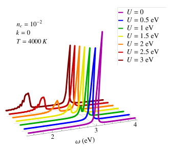
In Fig. 6 we illustrate the evolution of $G^{<}_{cc,0}(\omega)$ by varying the interaction strength $U$ (top panel) and the effective temperature $T$ (bottom panel) at fixed density $n_{c}=10^{-2}$. In the first case we clearly observe how the excitonic state develops. Starting from $U=0$ the exciton peak splits off from the qp peak and moves toward lower energies acquiring spectral weight and spreading over a finite energy window. If we lower the temperature at fixed $U$ the bottom panel indicates that the exciton peak shrinks and raises. However, the spectral weight $Z_{X}$ remains essentially constant (not shown). This suggests that the exciton peaks in TR-PE experiments should become more pronounced with increasing the delay between the pump and probe pulses since the excited electron liquid in the conduction band (initially very hot) has more time to cool down before getting probed.

Figure 7: Lesser Green’s function $-iG^{<}_{cc,k}(\omega)$ (in arbitrary units) for different momenta $k$ of the conduction electron. The (red) curve in the background is the integrated quantity $-i\int dk\,G^{<}_{cc,k}(\omega)$.

Figure 8: Momentum resolved and energy resolved excited spectral function $A_{k}(\omega)$ in arbitrary units. The dashed line corresponds to the exciton dispersion of the system in equilibrium.

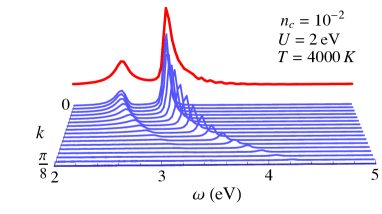
We have also calculated $G^{<}_{cc,k}(\omega)$ for different momenta $k$ of the conduction electron. This quantity is relevant to address angle-resolved experiments. In Fig. 7 we plot $-iG^{<}_{cc,k}(\omega)$ in the range $0<k<\pi/8$. For $k>\pi/8$ the lesser Green’s function is strongly suppressed by the Fermi function $f_{c}(\omega)$, see Eq. (74). It is interesting to observe that the angle-resolved photocurrent gives, in principle, access to the dispersion of the qp bound in an exciton. In order to better appreciate this point we show in Fig. 8 the spectral function $A_{k}(\omega)=i[G^{\rm R}_{cc,k}(\omega)-G^{\rm A}_{cc,k}(\omega)]$ for the same parameters of Fig. 7. From Eqs. (72) and (73) we expect that the peaks in $A_{k}(\omega)$ occur at the bare energy $\epsilon_{ck}$ and at $\epsilon_{vk-q}+\Omega^{Xq}$ where $\lambda=X$ labels the energy needed to excite an exciton of momentum $q$. In the quasi-stationary regime the residue $\bar{f}_{vk-q}\bar{F}^{\lambda q}+f_{vk-q}F^{\lambda q}$ of Eq. (72) is largest for $q\simeq k$ and hence the self-energy is dominated by the pole in $\epsilon_{v0}+\Omega^{Xk}$. The superimposed dashed line in Fig. 8 corresponds to the value of $\epsilon_{v0}+\Omega^{Xk}$ as obtained from an equilibrium calculation. More precisely we have solved Eq. (44) with equilibrium occupations and then identified $\Omega^{Xk}$ as the lowest (split-off) positive energy. If we write $\Omega^{Xk}=\epsilon_{ck}-\epsilon_{v0}-b_{X,k}^{\mathrm{eq}}$ (where $\epsilon_{ck}-\epsilon_{v0}$ is the noninteracting excitation energy) then $\epsilon_{v0}+\Omega^{Xk}=\epsilon_{ck}-b_{X,k}^{\mathrm{eq}}$. From Fig. 8 we see that $-iG^{<}_{cc,k}(\omega)$ is peaked in $\epsilon_{ck}$ and in the neighborhood of $\epsilon_{ck}-b_{X,q}^{\mathrm{eq}}$, thus confirming the physical picture that the bare conduction electron splits into a dressed conduction qp and into a bound qp. The discrepancy between the low-energy peak in $A_{k}(\omega)$ and the equilibrium calculation (dashed line) is due to the finite population of electrons in the conduction band. In general, the larger is $n_{c}$ and the more the bound qp dispersion differs from the one obtained by performing an equilibrium calculation. This points to the importance of solving the BSE with proper populations, as discussed in Section V.1. It is worth noting that the bound qp dispersion depends on the band structure of the solid and can differ substantially from the one of Fig. 8. Nevertheless, our theory is not limited to the minimal model of Eq. (75) and it can be applied to make predictions on real materials.

VII Summary and Conclusions

We developed a first-principles many-body diagrammatic approach to address TR and angle-resolved PE experiments in insulators and semiconductors with a low-energy spectrum dominated by exciton states. The time-dependent photocurrent can be calculated from a single-time convolution of the nonequilibrium lesser Green’s function and embedding self-energy. The latter is independent of the interaction and it is completely determined by the shape of the probe pulse and by the dipole matrix elements. The calculation of the lesser Green’s function does, in general, require the solution of the two-time Kadanoff-Baym equations.SvLbook ; KBbook ; KB.2000 ; DvL.2007 ; MSSvL.2009 ; BB.2013 ; PvFVA.2009 ; SBP.2016 ; SB.2016 However, if we are interested in probing the excited system after the pumped electrons have reached a thermal distribution (in the conduction band) then a quasi-stationary picture applies. In this regime one can solve the simpler one-time Kadanoff-Baym equations for the populations and then use these populations as inputs for the many-body approach presented in this work. The take-home message is that excitonic features in TR-PE emerge provided that (1) the self-energy diagram contains the HSEX vertex and (2) excited qp Green’s function are used to evaluate the self-energy diagrams.

The proposed theoretical framework has been applied to a minimal model Hamiltonian. We demonstrated that if the system is in a pure state with just one exciton then the many-body solution for the lesser Green’s function coincides with the exact solution. At finite temperatures we studied several features of the exciton peak. In addition to the intuitive red-shift with increasing the strength of the screened interaction we highlighted an asymmetric broadening which becomes more pronounced with increasing the density of electrons in the conduction band. We also showed that angle-resolved TR-PE spectroscopy can be used to calculate the bound qp dispersion and that this dispersion is in general different from the one obtained by solving the equilibrium BSE.

The proposed many-body approach is not the only first-principle method to tackle TR-PE spectra. Another popular method is Time-Dependent Density Functional Theory (TDDFT) which has already been applied to finite systemsDGBCWR.2013 ; LDGR.2016 ; WDGCR.2016 and, as it was recently shown, could be used for solids as well.BRPE.2016 However, in practical applications TDDFT is implemented with local functionals of time and space and the resulting spectrum is peaked at the Kohn-Sham single particle energies. This is not always satisfactory and the only remedy consists in developing ultra-nonlocal functionals as discussed in Ref. USvL.2014, . Our work clearly shows that local functionals cannot describe exciton peaks in TR-PE.

Finally we wish to point out that a first-principle approach to TR-PE experiments is crucial for the correct physical interpretation of the behavior of the spectral features as the intensity and envelop of the pump field is varied. Our work represents a first step in this direction and paves the way toward a more general theory and numerical approach to access the far-from-relaxed regime of the system during and shortly after the action of the pump.

Acknowledgements

We acknowledge financial support by the Futuro in Ricerca Grant No. RBFR12SW0J of the Italian Ministry of Education, University and Research MIUR. G.S. and E.P. also acknowledge EC funding through the RISE Co-ExAN (GA644076). D.S. and A.M. also acknowledge funding from the European Union project MaX Materials design at the eXascale H2020-EINFRA-2015-1, Grant Agreement No. 676598 and Nanoscience Foundries and Fine Analysis - Europe H2020-INFRAIA-2014-2015, Grant Agreement No. 654360.

References

- (1) K. Giesen, F. Hage, F. J. Himpsel, H. J. Riess, and W. Steinmann, Phys. Rev. Lett. 55, 300 (1995).
- (2) Th. Fauster and W. Steinmann, Photonic Probes of Surfaces, P. Halevi, Ed. (Elsevier, Amsterdam, 1995), pp. 347-411.
- (3) P. M. Echenique, R. Berndt, E. V. Chulkov, Th. Fauster, A. Goldmann, U.Höfer, Surf. Sci. Rep. 52, 219 (2004).
- (4) D. Varsano, M. A. L. Marques and A. Rubio, Comp. Mater. Sci. 30, 110 (2004).
- (5) D. Gugel, D. Niesner, C. Eickhoff, S. Wagner, M. Weinelt and T. Fauster, 2D Mater, 2, 045001 (2015).
- (6) W. S. Fann, R. Storz, H. W. K. Tom and J. Bokor, Phys. Rev. B 46, 13592 (1992).
- (7) H. Petek and S. Ogawa, Prog. Surf. Sci. 56, 239 (1997).
- (8) C. A. Schmuttenmaer, M. Aeschlimann, H. E. Elsayed-Ali, R. J. D. Miller, D. A. Mantell, J. Cao, and Y. Gao Phys. Rev. B 50, 8957(R) (2004).
- (9) M. Lisowski, P.A. Loukakos, U. Bovensiepen, J. Stähler, C. Gahl and M. Wolf, Appl. Phys. A 78, 165 (2004).
- (10) M. Weinelt, M. Kutschera, Th. Fauster and M. Rohlfing, Phys. Rev. Lett. 92, 126801 (2004).
- (11) T. Suzuki and R. Shimano, Phys. Rev. Lett. 103, 057401 (2009).
- (12) Z. Nie, R. Long, L. Sun, C.-C. Huang, J. Zhang, Q. Xiong, D. W. Hewak, Z. Shen, O. V. Prezhdo and Z.-H. Loh, ACS Nano 8, 10931 (2014).
- (13) H. Wang, C. Zhang, and F. Rana, Nano Lett. 15, 339 (2015).
- (14) J. Reimann, J. Güdde, K. Kuroda, E. V. Chulkov and U. Höfer, Phys. Rev. B 90, 081106(R) (2014).
- (15) J. A. Sobota, S. Yang, J. G. Analytis, Y. L. Chen, I. R. Fisher, P. S. Kirchmann and Z.-X. Shen, Phys. Rev. Lett. 108, 117403 (2012).
- (16) Y. H. Wang, D. Hsieh, E. J. Sie, H. Steinberg, D. R. Gardner, Y. S. Lee, P. Jarillo-Herrero and N. Gedik, Phys. Rev. Lett. 109, 127401 (2012).
- (17) A. Crepaldi, B. Ressel, F. Cilento, M. Zacchigna, C. Grazioli, H. Berger, Ph. Bugnon, K. Kern, M. Grioni and F. Parmigiani, Phys. Rev. B 86, 205133 (2012).
- (18) D. Niesner, S. Otto, V. Hermann, Th. Fauster, T. V. Menshchikova, S. V. Eremeev, Z. S. Aliev, I. R. Amiraslanov, M. B. Babanly, P. M. Echenique, and E. V. Chulkov, Phys. Rev. B 89, 081404(R) (2014).
- (19) M. Bernardi, D. Vigil-Fowler, J. Lischner, J. B. Neaton, and S. G. Louie, Phys. Rev. Lett. 112, 257402 (2014)
- (20) N.-H. Ge, C. M. Wong, R. L. Lingle Jr., J. D. McNeill, K. J. Gaffney and C. B. Harris, Science 279, 202 (1998).
- (21) T. Vondrak and X.-Y. Zhu, J. Phys. Chem. B 103, 3449 (1999).
- (22) M. Muntwiler, Q. Yang, W. A. Tisdale, and X.-Y. Zhu, Phys. Rev. Lett. 101, 196403 (2008).
- (23) X.-Y. Zhu, Q. Yang and M. Muntwiler, Acc. Chem. Res. 42 1779 (2009).
- (24) E. Varene, I. Martin and P. Tegeder, J. Phys. Chem. Lett. 2, 252 (2011).
- (25) T. Hannappel, B. Burfeindt, W. Storck and F. Willing, J. Phys. Chem. B 101, 6799 (1997).
- (26) J. Schnadt, P. A. Brḧwiler, L. Patthey, J. N. O’Shea, S. Södergren1, M. Odelius, R. Ahuja, O. Karis, M. Bässler, P. Persson, H. Siegbahn, S. Lunell and N. Mrtensson, Nature 418, 620 (2002).
- (27) Q. Zhong, C. Gahl and M, Wolf, Surf. Sci. 496, 21 (2002).
- (28) K. Onda, B. Li and H. Petek, Phys. Rev. B 70, 045415 (2004).
- (29) L. Miaja-Avila, G. Saathoff, S. Mathias, J. Yin, C. La-o-vorakiat, M. Bauer, M. Aeschlimann, M. M. Murnane and H. C. Kapteyn, Phys. Rev. Lett. 101, 046101 (2008).
- (30) T. L. Thompson and J. T. Yates Jr., Top. Catal. 35, 197 (2005).
- (31) D. M. Adams et al., J. Phys. Chem. B 107, 6668 (2003).
- (32) X.-Y. Zhu, J. El. Spec. Rel. Phenom. 204, 75 (2015).
- (33) V. Saile, D. Rieger, W. Steinmann and T. Wegehaupt, Phys. Lett. A 79, 221 (1980).
- (34) E. Varene, L. Bogner, C. Bronner, and P. Tegeder, Phys. Rev. Lett. 109, 207601 (2012).
- (35) J.-C. Deinert, D. Wegkamp, M. Meyer, C. Richter, M. Wolf and J. Stähler Phys. Rev. Lett. 113, 057602 (2014).
- (36) S. W. Koch, M. Kira, G. Khitrova and H. M. Gibbs, Nature Materials, 5, 523 (2006).
- (37) S. K. Sundaram and E. Mazur, Nature Materials 1, 217 (2002).
- (38) L. Bányai, D. B. Tran Thoai, E. Reitsamer, H. Haug, D. Steinbach, M. U. Wehner, M. Wegener, T. Marschner and W. Stolz, Phys. Rev. Lett. 75, 2188 (1995).
- (39) S. Bar-Ad and D. S. Chemla, Mater. Sci. Eng. B 48, 83 (1997).
- (40) D. Sangalli and A. Marini, J. Phys.: Conf. Series 609, 012006 (2015).
- (41) A. L. Fetter and J. D. Walecka, Quantum Theory of Many-Particle Systems (McGraw-Hill, New York, 1971)
- (42) G. Stefanucci and R. van Leeuwen, Nonequilibrium Many-Body Theory of Quantum Systems: A Modern Introduction (Cambridge University Press, 2013).
- (43) K. Ullrich, Time Dependent Density Functional Theory: Concepts and Applications (Oxford University Press, Oxford, 2012).
- (44) L. Hedin, Phys. Rev. 139, A796 (1965).
- (45) G. Strinati, Riv. Nuovo Cimento 11, 1 (1988).
- (46) G. Strinati, H. J. Mattausch, and W. Hanke, Phys. Rev. B 25, 2867 (1982).
- (47) G. Onida, L. Reining, and A. Rubio, Rev. Mod. Phys. 74, 601 (2002).
- (48) S. Albrecht, L. Reining, R. Del Sole, and G. Onida, Phys. Rev. Lett. 80, 4510 (1998).
- (49) L. X. Benedict, E. L. Shirley, and R. B. Bohn, Phys. Rev. Lett. 80, 4514 (1998).
- (50) M. Rohlfing and S. G. Louie, Phys. Rev. Lett. 81, 2312 (1998).
- (51) G. Pal, Y. Pavlyukh, W. Hübner, and H. C. Schneider, Eur. Phys. J. B 79, 327 (2011).
- (52) C. Attaccalite, M. Grüning and A. Marini, Phys. Rev. B 84, 245110 (2011).
- (53) E. Perfetto, D. Sangalli, A. Marini, and G. Stefanucci Phys. Rev. B 92, 205304 (2105).
- (54) A. Schleife, C. Rödl, F. Fuchs, K. Hannewald and F. Bechstedt, Phys. Rev. Lett. 107, 236405 (2011).
- (55) K. Hannewald, S. Glutsch, and F. Bechstedt, Phys. Rev. B 62, 4519 (2000).
- (56) C. Stampfl, K. Kambe, J. D. Riley and D. F. Lynch, J. Phys.: Condens. Matter 5, 8211 (1993).
- (57) N. Stojić, A. Dal Corso, B. Zhou and S. Baroni, Phys. Rev. B 77, 195116 (2008).
- (58) J. Braun, R. Rausch, M. Potthoff, J. Minár and H. Ebert, Phys. Rev. B 91, 035119 (2015).
- (59) H. J. Choi and J. Ihm, Phys. Rev. B 59, 2267 (1999).
- (60) A. Smogunov, A. Dal Corso, and E. Tosatti, Phys. Rev. B 70, 045417 (2004).
- (61) E. Perfetto, A.-M. Uimonen, R. van Leeuwen and G. Stefanucci, Phys. Rev. A 92, 033419 (2015).
- (62) M. Schüler, J. Berakdar and Y. Pavlyukh, Phys. Rev. B 93, 054303 (2016).
- (63) E. Perfetto, A.-M. Uimonen, R. van Leeuwen and G. Stefanucci, J. Phys.: Conf. Series 696, 012004 (2016).
- (64) Y. Meir and N. S. Wingreen, Phys. Rev. Lett. 68, 2512 (1992).
- (65) A.-P. Jauho, N. S. Wingreen, and Y. Meir, Phys. Rev. B 50, 5528 (1994).
- (66) G. Stefanucci and C.-O. Almbladh, Phys. Rev. B 69, 195318 (2004).
- (67) J. K. Freericks, H. R. Krishnamurthy and Th. Pruschke, Phys. Rev. Lett. 102, 136401 (2009).
- (68) The discussion can easily be generalized to situations where the system is left in an admixture of excited states.
- (69) L. P. Kadanoff and G. Baym, Quantum Statistical Mechanics (Benjamin, New York, 1962).
- (70) N.-H. Kwong and M. Bonitz, Phys. Rev. Lett. 84, 1768 (2000).
- (71) N. E. Dahlen and R. van Leeuwen, Phys. Rev. Lett. 98, 153004 (2007).
- (72) P. Myöhänen, A. Stan, G. Stefanucci and R. van Leeuwen, Phys. Rev. B 80, 115107 (2009).
- (73) K. Balzer, and M. Bonitz, Nonequilibrium Green’s Functions Approach to Inhomogeneous Systems, Lect. Notes Phys. vol. 867 (2013).
- (74) M. Puig von Friesen, C. Verdozzi and C.-O. Almbladh, Phys. Rev. Lett. 103, 176404 (2009).
- (75) N. Schlünzen and M. Bonitz, cond-mat/arXiv:1605.04588.
- (76) P. Lipavský, V. pika and B. Velický, Phys. Rev. B 34, 6933 (1986).
- (77) M. Bonitz, Quantum Kinetic Theory (B. G. Teubner Stuttgart, Leipzig, 1998).
- (78) H. Haug and A.-P. Jauho Quantum Kinetics in Transport and Optics of Semiconductors (Springer, Berlin, 2008).
- (79) M. Bonitz, D. Semkat and H. Haug, Eur. Phys. J. B 9, 309 (1999).
- (80) H. Haug and L. Bányai, Solid State Comm. 100, 303 (1996).
- (81) A. Marini, J. Phys.: Conf. Ser. 427, 012003 (2013).
- (82) S. Latini, E. Perfetto, A.-M. Uimonen, R. van Leeuwen and G. Stefanucci, Phys. Rev. B 89, 075306 (2014).
- (83) A. Marini, C. Hogan, M. Grüning and D. Varsano, Comp. Phys. Comm. 180, 1392 (2009).
- (84) D. Sangalli and A. Marini, EPL 110, 47004 (2015).
- (85) D. Sangalli, S. Dal Conte, C. Manzoni, G. Cerullo and A. Marini, Phys. Rev. B 93, 195205 (2016).
- (86) A. Stolow, A. E. Bragg and D. M. Neumark, Chem. Rev. 104, 1719 (2004)
- (87) M. Weinelt, A. B. Schmidt, M. Pickel, and M. Donath, Dynamics at Solid State Surfaces and Interfaces, Vol. 1: Current Developments (Wiley, New York, 2010).
- (88) H. Ueba and B. Gumhalter, Prog. Surf. Sci. 82, 193 (2007).
- (89) Z. Yang, Y. Li and C. Ullrich, J. Chem. Phys. 137, 014513 (2012).
- (90) U. De Giovannini, G. Brunetto, A. Castro, J. Walkenhorst and A. Rubio, Chem. Phys. Chem. 14, 1363 (2013).
- (91) A. H. Larsen , U. De Giovannini and A. Rubio, Top. Curr. Chem. 368, 219 (2016).
- (92) J. Walkenhorst, U. De Giovannini, A. Castro and A. Rubio, Eur. Phys. J. B 89, 1 (2016).
- (93) J. Braun, R. Rausch, M. Potthoff and H. Ebert, cond-mat/arXiv:1605.08596.
- (94) A.-M. Uimonen, G. Stefanucci, R. van Leeuwen, J. Chem. Phys. 140, 18A526 (2014).