OCU-PHYS 452

Dualities in ABJM Matrix Model
from Closed String Viewpoint


Kazuki Kiyoshige  and  Sanefumi Moriyama

Department of Physics, Graduate School of Science, Osaka City University
3-3-138 Sugimoto, Sumiyoshi, Osaka 558-8585, Japan

We propose a new formalism to study the ABJM matrix model. Contrary to expressing the fractional brane background with the Wilson loops in the open string formalism, we formulate the Wilson loop expectation value from the viewpoint of the closed string background. With this new formalism, we can prove some duality relations in the matrix model.

1 Introduction and summary

The most fundamental theory in theoretical physics is probably M-theory, which is an eleven-dimensional theory considered to unify all of the five ten-dimensional perturbative string theories. M2-branes and M5-branes are respectively fundamental and solitonic excitations in M-theory. From the fundamental roles it plays in theoretical physics, we naturally expect a large number of duality relations in M-theory. However, it is difficult to observe these dualities directly, since only little is known for this mysterious theory.

Recently, it was proposed [1, 2, 3] that the ${\mathcal{N}}=6$ superconformal Chern-Simons theory with gauge group U$(N_{1})\times$U$(N_{2})$, Chern-Simons levels $(k,-k)$ and two pairs of bifundamental matters describes the worldvolume theory of coincident $\min(N_{1},N_{2})$ M2-branes and $|N_{2}-N_{1}|$ fractional M2-branes on a geometry ${\mathbb{C}}^{4}/{\mathbb{Z}}_{k}$. The partition function and vacuum expectation values of the half-BPS Wilson loop on $S^{3}$, originally defined with the infinite-dimensional path integral, is reduced to a finite-dimensional matrix model [4]

$$\langle s_{Y}\rangle_{k}(N_{1},N_{2}) =\frac{(-1)^{\frac{1}{2}N_{1}(N_{1}-1)+\frac{1}{2}N_{2}(N_{2}-1)}}{N_{1}!N_{2}!}\int_{{\mathbb{R}}^{N_{1}+N_{2}}}\frac{d^{N_{1}}\mu}{(2\pi)^{N_{1}}}\frac{d^{N_{2}}\nu}{(2\pi)^{N_{2}}}e^{\frac{ik}{4\pi}(\sum_{m=1}^{N_{1}}\mu_{m}^{2}-\sum_{n=1}^{N_{2}}\nu_{n}^{2})}$$

$$\qquad\times\biggl{[}\frac{\prod_{m<m^{\prime}}^{N_{1}}2\sinh\frac{\mu_{m}-\mu_{m^{\prime}}}{2}\prod_{n<n^{\prime}}^{N_{2}}2\sinh\frac{\nu_{n}-\nu_{n^{\prime}}}{2}}{\prod_{m=1}^{N_{1}}\prod_{n=1}^{N_{2}}2\cosh\frac{\mu_{m}-\nu_{n}}{2}}\biggr{]}^{2}s_{Y}(e^{\mu}|e^{\nu}),$$ (1.1)

and a hidden super gauge group U$(N_{1}|N_{2})$ was observed [5, 2, 3, 4, 6]. Here $s_{Y}(x|y)$ is the supersymmetric Schur polynomial or the character of U$(N_{1}|N_{2})$. We directly observe a relation under the exchange of two sets of integration variables,

$$\langle s_{Y}\rangle_{k}(N_{1},N_{2})=\langle s_{Y^{\text{T}}}\rangle_{-k}(N_{2},N_{1})=[\langle s_{Y^{\text{T}}}\rangle_{k}(N_{2},N_{1})]^{*},$$ (1.2)

because of $s_{Y}(x|y)=s_{Y^{\text{T}}}(y|x)$. Hereafter we shall fix $k>0$. Also, we often consider the case of $M=N_{2}-N_{1}\geq 0$ unless otherwise stated and denote the expectation value $\langle s_{Y}\rangle_{k}(N,M+N)$ as $\langle s_{Y}\rangle_{k,M}(N)$.

It was then exciting to find that the partition function ([7, 8, 9, 11, 10, 12] for the case of equal ranks and [13, 14] for non-equal ranks) and vacuum expectation values of the half-BPS Wilson loop [15, 16] are respectively expressed in terms of the free energy of the closed and open topological string theories on local ${\mathbb{P}}^{1}\times{\mathbb{P}}^{1}$, which implies a certain modular invariance. Aside from the original computations in the ’t Hooft expansion [17, 18, 19], an important approach that leads to these findings is to rewrite the matrix model into the partition function of a Fermi gas system with $N$ non-interacting particles whose dynamics is governed by a non-trivial density matrix [8]. The success in formulating the partition function in terms of that of the Fermi gas system leads to a vast amount of WKB small $k$ expansions [8, 10] and numerical computations for finite $k$ [20, 21, 22, 9], from which the relation to the topological strings was found [7, 9, 12].

For the partition function in a general background with $M=N_{2}-N_{1}$ fractional branes, it was found that

$$\frac{\langle 1\rangle_{k,M}(N)}{\langle 1\rangle_{k,M}(0)}=\frac{1}{N!}\int\frac{d^{N}x}{(4\pi k)^{N}}\prod_{i<j}^{N}\biggl{(}\tanh\frac{x_{i}-x_{j}}{2k}\biggr{)}^{2}\prod_{i=1}^{N}V_{M}(x_{i}),$$ (1.3)

where $V_{M}(x)$ is defined as

$$V_{M}(x)=\frac{1}{2\cosh\frac{x}{2}}\prod_{\overline{l}\in\overline{L}}\tanh\frac{x+2\pi i\overline{l}}{2k},$$ (1.4)

with $\overline{L}=\{M-\frac{1}{2},M-\frac{3}{2},\cdots,\frac{3}{2},\frac{1}{2}\}$. If we introduce the coordinate and momentum operators satisfying the canonical commutation relation $[\widehat{q},\widehat{p}]=i\hbar$ with $\hbar=2\pi k$, the grand canonical partition function $\langle 1\rangle^{\text{GC}}_{k,M}(z)=\sum_{N=0}^{\infty}z^{N}\langle 1\rangle_{k,M}(N)$ is expressed as

$$\frac{\langle 1\rangle^{\text{GC}}_{k,M}(z)}{\langle 1\rangle_{k,M}(0)}=\det(1+z\widehat{\rho}_{M}),$$ (1.5)

with the density matrix $\widehat{\rho}_{M}$ given by

$$\widehat{\rho}_{M}=\sqrt{V_{M}(\widehat{q})}\frac{1}{2\cosh\frac{\widehat{p}}{2}}\sqrt{V_{M}(\widehat{q})}.$$ (1.6)

The expression (1.3) was first found for the case of equal ranks $M=0$ in [8] and later extended to the case of non-equal ranks. Namely, for $M\neq 0$, (1.3) was originally conjectured in [23] and proved in [24] with several steps of integrations. In this paper we shall rederive the result with a more refined presentation motivated by [25, 26] as a byproduct of our analysis.

In the expansion of the determinant in (1.5) there appear many traces of powers of the density matrix $\widehat{\rho}_{M}$. In introducing a background with $M$ fractional branes, all we have to do is to modify the density matrix $\widehat{\rho}_{M}$ (1.6) by changing $V_{M=0}(x)$ into $V_{M}(x)$ (1.4) without touching the structure of the determinant. In other words, we express the fractional branes by dressing the density matrix so that the background where the closed strings propagate is changed. From this viewpoint, this formalism is called “closed string formalism” in [27].

Since some poles of $(2\cosh\frac{x}{2})^{-1}$ in (1.4) at $x\in 2\pi i({\mathbb{Z}}\pm\frac{1}{2})$ are cancelled by the zeros of the hyperbolic tangent functions at $x=-2\pi i\overline{l}$, we can shift the integration contour by $-M\pi i$ [14]. This shift is essential to make contact with the orthosymplectic Chern-Simons matrix model [28, 29, 30, 31, 25, 26]. This matrix model is obtained from the localization of the ${\mathcal{N}}=5$ superconformal Chern-Simons theory with the orthosymplectic gauge group [2, 3] and the physical interpretation is the introduction of the orientifold plane in the type IIB setup. In [30, 25, 26] it was proved that the partition function of the orthosymplectic Chern-Simons matrix model is nothing but the chiral projection of the Chern-Simons matrix model with the super unitary gauge group (see table 1 in [26] for an interesting pattern).

There is another formalism to study the matrix model [13] called “open string formalism”. Here we do not change the expression of the density matrix from the $M=0$ case and instead introduce many extra contributions with endpoints. In this sense, as the Wilson loop expectation values [16], we express the fractional brane background with the open string endpoints. At present we stress that the open string formalism seems superior to the closed string one because it is obtained only from the combinatorics and hence is applicable not only for the partition function but also with the Wilson loop insertion. In this formalism the expectation values of the half-BPS Wilson loop in the grand canonical ensemble

$$\langle s_{Y}\rangle^{\text{GC}}_{k,M}(z)=\sum_{N=r}^{\infty}z^{N-r}\langle s_{Y}\rangle_{k,M}(N),$$ (1.7)

is reduced to

$$\frac{\langle s_{Y}\rangle^{\text{GC}}_{k,M}(z)}{\langle 1\rangle^{\text{GC}}_{k,0}(z)}=\det\begin{pmatrix}\bigl{(}H_{l_{p},-M+q-\frac{1}{2}}(z)\bigr{)}_{(M+r)\times M}&\bigl{(}\widetilde{H}_{l_{p},a_{q}}(z)\bigr{)}_{(M+r)\times r}\end{pmatrix},$$ (1.8)

where both $H_{l,a}(z)$ and $\widetilde{H}_{l,a}(z)$ take the form of a certain matrix element of $[1+z\widehat{\rho}_{M=0}]^{-1}$ (see [13] for the explicit form). The indices $a_{q}$, $l_{p}$ in (1.8) are the arm lengths and the leg lengths appearing in the Frobenius notation, which is another description of the Young diagram usually described by listing all of the arm lengths $[\alpha_{1},\alpha_{2},\cdots]$ or the leg lengths $[\lambda_{1},\lambda_{2},\cdots]^{\text{T}}$,

$$a_{q}=\alpha_{q}-q-M+1/2,\quad l_{p}=\lambda_{p}-p+M+1/2,$$

$$r=\max\{q|a_{q}>0\}=\max\{p|l_{p}>0\}-M.$$ (1.9)

See figure 1 for a pictorial explanation of the Frobenius notation. Note that here we have deliberately added $\frac{1}{2}$ to the lengths to measure the distances between the midpoints of two segments. As stressed in [16, 35], the integrations in $H_{l,a}(z)$ and $\widetilde{H}_{l,a}(z)$ are convergent only for $a_{1}+l_{1}<k/2$ (which implies $M\leq k/2$). We shall follow this condition in our analysis. One advantage of the open string formalism (1.8) is that we can prove the Giambelli compatibility for $\langle s_{Y}\rangle^{\text{GC}}_{k,M}(z)$ generally when correctly normalized with $\langle 1\rangle^{\text{GC}}_{k,M}(z)$ [36].

Although many identities were proved in this context, still a lot of important duality relations await to be proved. One of them is the miraculous open-closed duality observed recently in [35]. In [35], motivated by [37], starting from the simplest case with $r=1,M=0$, the authors arrive at a more general relation

$$\langle s_{[(M+r)^{r}]}\rangle^{\text{GC}}_{k,M}(z)\sim\langle 1\rangle^{\text{GC}}_{k,M+2r}(z),$$ (1.10)

with numerical computations. Here $\sim$ means that the relation holds up to a numerical factor independent of $z$. This duality relates the closed string BPS indices to the open string BPS indices and is another realization of the spirit of the open string formalism [13], which expresses the closed string background formed by fractional branes with many open strings in the determinant. In the same paper, the authors also observe a relation

$$\langle s_{(a|l)}\rangle^{\text{GC}}_{k,M}(z)\sim[\langle s_{(l+M|a-M)}\rangle^{\text{GC}}_{k,M}(z)]^{*},$$ (1.11)

for the hook representation $(a|l)$ with $a>M$. The complex conjugation applies only for the coefficients of $z$.

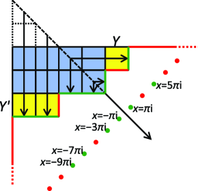
Figure 1: Young diagram and Frobenius notation. The standard Frobenius notation is defined by counting the boxes from the diagonal line. For the super case U$(N_{1}|N_{2})$, we shift the diagonal line by $M=N_{2}-N_{1}$. For the Young diagram in the figure $[\alpha_{1},\alpha_{2},\alpha_{3}]=[5,4,2]$ or $[\lambda_{1},\lambda_{2},\lambda_{3},\lambda_{4},\lambda_{5}]^{\text{T}}=[3,3,2,2,1]^{\text{T}}$, the standard Frobenius notation is $(42|21)$ and the shifted one with $M=2$ is $(20|4310)$. Here we find it useful to define the arm and leg lengths by adding $\frac{1}{2}$, or in other words, measuring the distances between the midpoints of two segments, $(a_{1},a_{2}|l_{1},l_{2},l_{3},l_{4})=(\frac{5}{2},\frac{1}{2}|\frac{9}{2},\frac{7}{2},\frac{3}{2},\frac{1}{2})$. We sometimes decompose the Young diagram as $([(M+r)^{r}]+Y)\cup Y^{\prime}$, which in the current case is $([4^{2}]+[1])\cup[2]$. We also display the poles of $(2\cosh\frac{x}{2})^{-1}$ in (1.13) in our Fermi gas formalism (1.12). The green dots denote the poles at $x=2\pi ia$ and $x=-2\pi il$ which are cancelled by the hyperbolic tangent functions in (1.13) and hence harmless, while the red dots denote the real poles which are not cancelled.

In this paper, we shall generalize the closed string formalism (1.3), so that it incorporates the Wilson loop insertion. Namely, contrary to the open string formalism [13] where we describe the fractional brane as a composite of the Wilson loops, here we propose an opposite formalism, which describes the Wilson loop by changing the closed string backgrounds,

$$\frac{\langle s_{Y}\rangle_{k,M}(N)}{\langle s_{Y}\rangle_{k,M}(r)}=\frac{1}{(N-r)!}\int\frac{d^{N-r}x}{(4\pi k)^{N-r}}\prod_{i<j}^{N-r}\biggl{(}\tanh\frac{x_{i}-x_{j}}{2k}\biggr{)}^{2}\prod_{i=1}^{N-r}V(x_{i}),$$ (1.12)

with

$$V(x)=\frac{1}{2\cosh\frac{x}{2}}\prod_{a\in A}\tanh\frac{x-2\pi ia}{2k}\prod_{l\in L}\tanh\frac{x+2\pi il}{2k}.$$ (1.13)

Here $A$ and $L$ denote respectively the set of all arm lengths and all leg lengths of the Young diagram $Y$. Note that $\overline{L}$ appearing in (1.4) is the set of all leg lengths in the trivial representation. From (1.13) it is easy to observe that although $x\in 2\pi i({\mathbb{Z}}\pm\frac{1}{2})$ are poles potentially, poles at $x=2\pi ia$ and $x=-2\pi il$ are cancelled by the zeros of the hyperbolic tangent functions (see figure 1). Also, since $a_{1}+l_{1}<k/2$, a hyperbolic tangent does not induce a new pole at the zero of another hyperbolic tangent.

Using this new formalism we are able to prove some untouched dualities without difficulties. Here we prove a generalized open-closed duality

$$\langle s_{([(M+r)^{r}]+Y)\cup Y^{\prime}}\rangle^{\text{GC}}_{k,M}(z)\sim\langle s_{([(M+r-1)^{r+1}]+Y)\cup Y^{\prime}}\rangle^{\text{GC}}_{k,M-2}(z).$$ (1.14)

In fact, from the expression (1.12) it is not difficult to find that we can shift the integration contour as long as we do not cross the poles. Due to this reason, the expectation values of two Young diagrams in the grand canonical ensemble, which share the same set of

$$\{a_{q}|q=1,\cdots,r\}\cup\{-l_{p}|p=1,\cdots,M+r\},$$ (1.15)

up to an overall shift of an integer, are identical.

This paper is organized as follows. In the next section, we propose a new formalism to study the Wilson loop expectation values. In section 3, we use this formalism to prove (a generalized version of) the open-closed duality. Finally in section 4, we conclude with discussions on the future directions.

2 Wilson loop as closed string background

In this section, following the method developed in [25, 26], we shall rewrite the expectation value of the half-BPS Wilson loop (1.1) into the partition function of a new Fermi gas system, where the density matrix is modified while the determinant structure is kept fixed. We shall rescale the integration variables by $k$ as

$$\langle s_{Y}\rangle_{k,M}(N) =\frac{(-1)^{\frac{1}{2}N_{1}(N_{1}-1)+\frac{1}{2}N_{2}(N_{2}-1)}}{N_{1}!N_{2}!}\int\frac{d^{N_{1}}\mu}{\hbar^{N_{1}}}\frac{d^{N_{2}}\nu}{\hbar^{N_{2}}}e^{\frac{i}{2\hbar}(\sum_{m=1}^{N_{1}}\mu_{m}^{2}-\sum_{n=1}^{N_{2}}\nu_{n}^{2})}$$

$$\qquad\times\biggl{[}\frac{\prod_{m<m^{\prime}}^{N_{1}}2\sinh\frac{\mu_{m}-\mu_{m^{\prime}}}{2k}\prod_{n<n^{\prime}}^{N_{2}}2\sinh\frac{\nu_{n}-\nu_{n^{\prime}}}{2k}}{\prod_{m=1}^{N_{1}}\prod_{n=1}^{N_{2}}2\cosh\frac{\mu_{m}-\nu_{n}}{2k}}\biggr{]}^{2}s_{Y}(e^{\frac{\mu}{k}}|e^{\frac{\nu}{k}}),$$ (2.1)

with $\hbar=2\pi k$ and $k>0$. We begin our analysis by assuming $M=N_{2}-N_{1}\geq 0$ and denote $N_{1}=N$, $N_{2}=M+N$ and $\langle s_{Y}\rangle_{k}(N,M+N)=\langle s_{Y}\rangle_{k,M}(N)$.

As in the open string formalism [13], our starting point is the following three determinant formulas; the Cauchy-Vandermonde determinant

$$\frac{\prod_{m<m^{\prime}}^{N_{1}}(x_{m}-x_{m^{\prime}})\prod_{n<n^{\prime}}^{N_{2}}(y_{n}-y_{n^{\prime}})}{\prod_{m=1}^{N_{1}}\prod_{n=1}^{N_{2}}(x_{m}+y_{n})}=(-1)^{N_{1}(N_{2}-N_{1})}\det\begin{pmatrix}\biggl{[}\displaystyle\frac{1}{x_{m}+y_{n}}\biggr{]}_{(m,n)\in Z_{1}\times Z_{2}}\\ \Bigl{[}y_{n}^{\overline{l}-\frac{1}{2}}\Bigr{]}_{(\overline{l},n)\in\overline{L}\times Z_{2}}\end{pmatrix},$$ (2.2)

where $m$, $n$ and $\overline{l}$ are respectively elements of $Z_{1}=\{1,2,\cdots,N_{1}\}$, $Z_{2}=\{1,2,\cdots,N_{2}\}$ and $\overline{L}=\{M-\frac{1}{2},M-\frac{3}{2},\cdots,\frac{1}{2}\}$ in this order; the same determinant

$$(-1)^{\frac{1}{2}N_{1}(N_{1}-1)+\frac{1}{2}N_{2}(N_{2}-1)}\frac{\prod_{m<m^{\prime}}^{N_{1}}(x_{m^{\prime}}^{-1}-x_{m}^{-1})\prod_{n<n^{\prime}}^{N_{2}}(y_{n^{\prime}}^{-1}-y_{n}^{-1})}{\prod_{m=1}^{N_{1}}\prod_{n=1}^{N_{2}}(x_{m}^{-1}+y_{n}^{-1})}$$

$$=(-1)^{N_{1}(N_{2}-N_{1})}\det\begin{pmatrix}\biggl{[}\displaystyle\frac{1}{y_{n}^{-1}+x_{m}^{-1}}\biggr{]}_{(n,m)\in Z_{2}\times Z_{1}}&\Bigl{[}y_{n}^{-\overline{l}+\frac{1}{2}}\Bigr{]}_{(n,\overline{l})\in Z_{2}\times\overline{L}}\end{pmatrix},$$ (2.3)

obtained by the substitutions $x_{m}\to x_{m}^{-1}$ and $y_{n}\to y_{n}^{-1}$; the determinantal formula for the supersymmetric Schur polynomial due to Moens and Van der Jeugt [38]

$$\frac{s_{Y}(x|y)}{(-1)^{r}}=\det\begin{pmatrix}\biggl{[}\displaystyle\frac{1}{x_{m}+y_{n}}\biggr{]}_{(m,n)\in Z_{1}\times Z_{2}}&\Bigl{[}x_{m}^{a-\frac{1}{2}}\Bigr{]}_{(m,a)\in Z_{1}\times A}\\ \Bigl{[}y_{n}^{l-\frac{1}{2}}\Bigr{]}_{(l,n)\in L\times Z_{2}}&[0]_{L\times A}\end{pmatrix}\bigg{/}\det\begin{pmatrix}\biggl{[}\displaystyle\frac{1}{x_{m}+y_{n}}\biggr{]}_{(m,n)\in Z_{1}\times Z_{2}}\\ \Bigl{[}y_{n}^{\overline{l}-\frac{1}{2}}\Bigr{]}_{(\overline{l},n)\in\overline{L}\times Z_{2}}\end{pmatrix},$$ (2.4)

with $A=\{a_{1},a_{2},\cdots,a_{r}\}$ and $L=\{l_{1},l_{2},\cdots,l_{M+r}\}$, where, as in figure 1, the arm and leg lengths measure the distances between the midpoints of two segments and are greater than the standard ones by $\frac{1}{2}$. After multiplying these three formulas with the substitutions $x_{m}=e^{\frac{\mu_{m}}{k}}$ and $y_{n}=e^{\frac{\nu_{n}}{k}}$, we find

$$(-1)^{\frac{1}{2}N_{1}(N_{1}-1)+\frac{1}{2}N_{2}(N_{2}-1)}\biggl{[}\frac{\prod_{m<m^{\prime}}^{N_{1}}2\sinh\frac{\mu_{m}-\mu_{m^{\prime}}}{2k}\prod_{n<n^{\prime}}^{N_{2}}2\sinh\frac{\nu_{n}-\nu_{n^{\prime}}}{2k}}{\prod_{m=1}^{N_{1}}\prod_{n=1}^{N_{2}}2\cosh\frac{\mu_{m}-\nu_{n}}{2k}}\biggr{]}^{2}\frac{s_{Y}(e^{\frac{\mu}{k}}|e^{\frac{\nu}{k}})}{(-1)^{r}}$$

$$=\det\begin{pmatrix}\biggl{[}\displaystyle\frac{1}{2\cosh\frac{\mu_{m}-\nu_{n}}{2k}}\biggr{]}_{N_{1}\times N_{2}}&\bigl{[}e^{\frac{a\mu_{m}}{k}}\bigr{]}_{N_{1}\times r}\\ \bigl{[}e^{\frac{l\nu_{n}}{k}}\bigr{]}_{(M+r)\times N_{2}}&[0]_{(M+r)\times r}\end{pmatrix}\det\begin{pmatrix}\biggl{[}\displaystyle\frac{1}{2\cosh\frac{\nu_{n}-\mu_{m}}{2k}}\biggr{]}_{N_{2}\times N_{1}}&\bigl{[}e^{-\frac{\overline{l}\nu_{n}}{k}}\bigr{]}_{N_{2}\times M}\end{pmatrix}.$$ (2.5)

Next, let us rewrite the components of the determinants by using the Fourier transformation of $(2\cosh\frac{\widehat{p}}{2})^{-1}$ and introducing the formal states $|h\operatorname{\!\rangle\!\rangle}$ and $\operatorname{\langle\!\langle\!}h|$ as in [25], $(h\in{\mathbb{Z}}\pm\frac{1}{2})$

$$\langle\mu|\frac{1}{2\cosh\frac{\widehat{p}}{2}}|\nu\rangle=\frac{1}{k}\frac{1}{2\cosh\frac{\mu-\nu}{2k}},\qquad\operatorname{\langle\!\langle\!}h|\mu\rangle=\langle\mu|h\operatorname{\!\rangle\!\rangle}=e^{\frac{h\mu}{k}}.$$ (2.6)

Then, we can follow the standard tricks of including the Gaussian factor into the brackets and applying the similarity transformation

$$1=\int\frac{dq}{2\pi}|q\rangle\langle q|\quad\Rightarrow\quad 1=\int\frac{dq}{2\pi}e^{-\frac{i}{2\hbar}\widehat{p}^{2}}|q\rangle\langle q|e^{\frac{i}{2\hbar}\widehat{p}^{2}},$$ (2.7)

to the $\mu$ and $\nu$ integrations. After these manipulations, the expectation value is expressed as

$$\langle s_{Y}\rangle_{k,M}(N)=\frac{(-1)^{r}}{N_{1}!N_{2}!}\int\frac{d^{N_{1}}\mu}{\hbar^{N_{1}}}\frac{d^{N_{2}}\nu}{\hbar^{N_{2}}}$$

$$\quad\times\det\begin{pmatrix}\biggl{[}\displaystyle k\langle\mu_{m}|e^{\frac{i}{2\hbar}\widehat{p}^{2}}e^{\frac{i}{2\hbar}\widehat{q}^{2}}\frac{1}{2\cosh\frac{\widehat{p}}{2}}e^{-\frac{i}{2\hbar}\widehat{q}^{2}}e^{-\frac{i}{2\hbar}\widehat{p}^{2}}|\nu_{n}\rangle\biggr{]}_{N_{1}\times N_{2}}&\Bigl{[}\langle\mu_{m}|e^{\frac{i}{2\hbar}\widehat{p}^{2}}e^{\frac{i}{2\hbar}\widehat{q}^{2}}|a\operatorname{\!\rangle\!\rangle}\Bigr{]}_{N_{1}\times r}\\ \Bigl{[}\operatorname{\langle\!\langle\!}l|e^{-\frac{i}{2\hbar}\widehat{q}^{2}}e^{-\frac{i}{2\hbar}\widehat{p}^{2}}|\nu_{n}\rangle\Bigr{]}_{(M+r)\times N_{2}}&\bigl{[}0\bigr{]}_{(M+r)\times r}\end{pmatrix}$$

$$\quad\times\det\begin{pmatrix}\biggl{[}\displaystyle k\langle\nu_{n}|e^{\frac{i}{2\hbar}\widehat{p}^{2}}\frac{1}{2\cosh\frac{\widehat{p}}{2}}e^{-\frac{i}{2\hbar}\widehat{p}^{2}}|\mu_{m}\rangle\biggr{]}_{N_{2}\times N_{1}}&\Bigl{[}\langle\nu_{n}|e^{\frac{i}{2\hbar}\widehat{p}^{2}}|{-\overline{l}}\operatorname{\!\rangle\!\rangle}\Bigr{]}_{N_{2}\times M}\end{pmatrix}.$$ (2.8)

It is magical [25] that all of the components in the first determinant reduce to delta functions

$$k\langle\mu|e^{\frac{i}{2\hbar}\widehat{p}^{2}}e^{\frac{i}{2\hbar}\widehat{q}^{2}}\frac{1}{2\cosh\frac{\widehat{p}}{2}}e^{-\frac{i}{2\hbar}\widehat{q}^{2}}e^{-\frac{i}{2\hbar}\widehat{p}^{2}}|\nu\rangle =\frac{\hbar}{2\cosh\frac{\mu}{2}}\delta(\mu-\nu),$$

$$\langle\mu|e^{\frac{i}{2\hbar}\widehat{p}^{2}}e^{\frac{i}{2\hbar}\widehat{q}^{2}}|a\operatorname{\!\rangle\!\rangle} =\frac{\hbar}{\sqrt{-ik}}e^{\frac{i}{2\hbar}(2\pi a)^{2}}\delta(\mu-2\pi ia),$$

$$\operatorname{\langle\!\langle\!}l|e^{-\frac{i}{2\hbar}\widehat{q}^{2}}e^{-\frac{i}{2\hbar}\widehat{p}^{2}}|\nu\rangle =\frac{\hbar}{\sqrt{ik}}e^{-\frac{i}{2\hbar}(2\pi l)^{2}}\delta(\nu+2\pi il).$$ (2.9)

For the second determinant we have

$$\langle\nu|e^{\frac{i}{2\hbar}\widehat{p}^{2}}|{-\overline{l}}\operatorname{\!\rangle\!\rangle} =e^{-\frac{i}{2\hbar}(2\pi\overline{l})^{2}}\langle\nu|{-\overline{l}}\operatorname{\!\rangle\!\rangle}.$$ (2.10)

For the expansion of the first determinant to be non-vanishing we need to choose $r$ rows out of $N$ rows in the upper-right block and $M+r$ columns out of $M+N$ columns in the lower-left block. Then, the remaining $N-r$ components are chosen from the upper-left block. In renaming the indices, we have $r!(M+r)!(N-r)!$ identical terms with signs $(-1)^{(M+r)r}$. After combining these factors, we find

$$\langle s_{Y}\rangle_{k,M}(N)=\frac{(-1)^{\frac{1}{2}M(M-1)+Mr}}{(N-r)!}\int\frac{d^{N}\mu}{\hbar^{N}}\frac{d^{M+N}\nu}{\hbar^{M+N}}e^{\frac{i}{2\hbar}(2\pi)^{2}(\sum a^{2}-\sum l^{2}-\sum\overline{l}^{2})}$$

$$\qquad\times\prod_{i=1}^{N-r}\frac{\hbar}{2\cosh\frac{\mu_{i}}{2}}\delta(\mu_{i}-\nu_{i})\prod_{q=1}^{r}\frac{\hbar}{\sqrt{-ik}}\delta(\mu_{N-r+q}-2\pi ia_{q})\prod_{p=1}^{M+r}\frac{\hbar}{\sqrt{ik}}\delta(\nu_{N-r+p}+2\pi il_{p})$$

$$\qquad\times e^{\frac{M}{2k}(\sum_{m=1}^{N}\mu_{m}-\sum_{n=1}^{M+N}\nu_{n})}\frac{\prod_{m<m^{\prime}}^{N}2\sinh\frac{\mu_{m}-\mu_{m^{\prime}}}{2k}\prod_{n<n^{\prime}}^{M+N}2\sinh\frac{\nu_{n}-\nu_{n^{\prime}}}{2k}}{\prod_{m=1}^{N}\prod_{n=1}^{M+N}2\cosh\frac{\mu_{m}-\nu_{n}}{2k}},$$ (2.11)

where we have used $(-1)^{r^{2}}=(-1)^{r}$. After performing the integration of the delta functions by substitutions, we arrive at the expression

$$\frac{\langle s_{Y}\rangle_{k,M}(N)}{\langle s_{Y}\rangle_{k,M}(r)}=\frac{1}{(N-r)!}\int\frac{d^{N-r}x}{(4\pi k)^{N-r}}\prod_{i<j}^{N-r}\biggl{(}\tanh\frac{x_{i}-x_{j}}{2k}\biggr{)}^{2}$$

$$\qquad\times\prod_{i=1}^{N-r}\biggl{[}\frac{1}{2\cosh\frac{x_{i}}{2}}\prod_{a\in A}\tanh\frac{x_{i}-2\pi ia}{2k}\prod_{l\in L}\tanh\frac{x_{i}+2\pi il}{2k}\biggr{]},$$ (2.12)

where the normalization is given by

$$\langle s_{Y}\rangle_{k,M}(r) =\frac{i^{\frac{1}{2}M(M-1)+Mr}e^{\frac{\pi i}{k}(\sum a^{2}-\sum l^{2}-\sum\overline{l}^{2})}e^{\frac{\pi i}{k}M(\sum a+\sum l)}}{\sqrt{-ik}^{r}\sqrt{ik}^{M+r}}\frac{\prod_{a>a^{\prime}}2\sin\frac{\pi(a-a^{\prime})}{k}\prod_{l>l^{\prime}}2\sin\frac{\pi(l-l^{\prime})}{k}}{\prod_{a}\prod_{l}2\cos\frac{\pi(a+l)}{k}}.$$ (2.13)

We note that, although we originally start with the situation of $N_{1}\leq N_{2}$, both of the formulas (2.12) and (2.13) are valid for the opposite case $N_{1}>N_{2}$ as well if we stick to the original notation $N_{1}=N$, $N_{2}=M+N$, $\max\{q|a_{q}>0\}=r$, $\max\{p|l_{p}>0\}=M+r$ and $\langle s_{Y}\rangle_{k,M}(N)=\langle s_{Y}\rangle_{k}(N,M+N)$ but $M<0$. Therefore, no special care is needed when crossing the diagonal line and we can extend to $M<0$ directly.

Finally let us comment on the closed string formalism for the partition function (1.3). In [24] the proof was done by several steps of integrations. Following the method of [25, 26], we have generalized the formalism for the expectation values of the half-BPS Wilson loop. The result of the partition function can be simply rederived by setting $A=\emptyset,L=L^{\prime}$ in (2.12).

3 Proof of generalized open-closed duality

In the previous section we have found that, after suitably normalized, the expectation value $\langle s_{Y}\rangle_{k,M}(N)$ is given in (1.12) with $V(x)$ defined by (1.13) and no special care is needed when crossing $M=0$. From figure 1 we know that $V(x)$ contains poles periodically, though some of them are cancelled by the zeros of the hyperbolic tangent functions. Therefore, as long as we do not encounter the real poles, we can shift the integration contour or in contrast the position of the poles by $\pm 2\pi i$ freely, so that two expectation values which share the same set of (1.15) up to an integral shift are identical. This identity induces the duality relation we want to prove. Let us see this explicitly for the example in figure 1. Here we assume that $k$ is large enough so that we do not have to consider the poles of the hyperbolic tangent functions in our shift of the integration contour.

In figure 2 we pick up the example in figure 1 and shift the integration contour in the unit of $2\pi i$. Starting from $(\frac{5}{2},\frac{1}{2}|\frac{9}{2},\frac{7}{2},\frac{3}{2},\frac{1}{2})$, if we move the integration coutour upwards (so that the number of leg lengths increases), we find $(\frac{3}{2}|\frac{11}{2},\frac{9}{2},\frac{5}{2},\frac{3}{2},\frac{1}{2})$, where in this shift we only move across the harmless green pole ($x=\pi i$ in figure 1) and the expectation value is not changed. If we move further into $(\frac{1}{2}|\frac{13}{2},\frac{11}{2},\frac{7}{2},\frac{5}{2},\frac{3}{2})$, now we need to cross the real red pole ($x=3\pi i$ in figure 1) and the expectation value is changed. Similarly, we can move downwards to $(\frac{7}{2},\frac{3}{2},\frac{1}{2}|\frac{7}{2},\frac{5}{2},\frac{1}{2})$ and so on without changing the expectation values for a while. We have classified the expectation values by the shaded green backgrounds in figure 2.

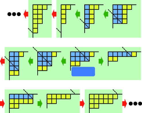
Figure 1

Figure 2: Shifting the integration contour across the harmless poles does not change the expectation values and hence induces the duality, while shifting across the poles is not allowed. We assume that $k$ is large enough.

We can summarize the above duality relation as

$$\frac{\langle s_{([(M+r)^{r}]+Y)\cup Y^{\prime}}\rangle^{\text{GC}}_{k,M}(z)}{\langle s_{([(M+r)^{r}]+Y)\cup Y^{\prime}}\rangle_{k,M}(r)}=\frac{\langle s_{([(M+r-1)^{r+1}]+Y)\cup Y^{\prime}}\rangle^{\text{GC}}_{k,M-2}(z)}{\langle s_{([(M+r-1)^{r+1}]+Y)\cup Y^{\prime}}\rangle_{k,M-2}(r+1)},$$ (3.1)

if $\lambda_{1}\leq r$ and $\alpha_{1}\leq M+r-1$ where $\lambda_{1}=\lambda_{1}(Y)$ and $\alpha_{1}=\alpha_{1}(Y^{\prime})$ denote the first leg length of $Y$ and the first arm length of $Y^{\prime}$. Using this recursively, we find

$$\frac{\langle s_{([(\widetilde{M}-\lambda_{1})^{\lambda_{1}}]+Y)\cup Y^{\prime}}\rangle^{\text{GC}}_{k,\widetilde{M}-2\lambda_{1}}(z)}{\langle s_{([(\widetilde{M}-\lambda_{1})^{\lambda_{1}}]+Y)\cup Y^{\prime}}\rangle_{k,\widetilde{M}-2\lambda_{1}}(\lambda_{1})}=\frac{\langle s_{([(\alpha_{1})^{\widetilde{M}-\alpha_{1}}]+Y)\cup Y^{\prime}}\rangle^{\text{GC}}_{k,-\widetilde{M}+2\alpha_{1}}(z)}{\langle s_{([(\alpha_{1})^{\widetilde{M}-\alpha_{1}}]+Y)\cup Y^{\prime}}\rangle_{k,-\widetilde{M}+2\alpha_{1}}(\widetilde{M}-\alpha_{1})},$$ (3.2)

with $\widetilde{M}=M+2r$. For the special case $\lambda_{1}=\alpha_{1}=0$ this reduces to (1.10).

In [35] another interesting identity (1.11)

$$\frac{\langle s_{(a|l)}\rangle^{\text{GC}}_{k,M}(z)}{\langle s_{(a|l)}\rangle_{k,M}(1)}=\biggl{[}\frac{\langle s_{(l+M|a-M)}\rangle^{\text{GC}}_{k,M}(z)}{\langle s_{(l+M|a-M)}\rangle_{k,M}(1)}\biggr{]}^{*},$$ (3.3)

with $a>M$ was found numerically. However, after generalizing the open-closed duality into (3.2), we point out that this falls into the same class of the identity. Namely, since the Young diagram $(a|l)$ is decomposed as $([(M+1)^{1}]+[a-M-\frac{1}{2}])\cup[1^{l-\frac{1}{2}}]$, we can use our formula (3.2) to shift the integration contour to obtain $([1^{M+1}]+[a-M-\frac{1}{2}])\cup[1^{l-\frac{1}{2}}]$, which is $(a-M|l+M)$. After applying the conjugate relation (1.2), this reduces to (3.3).

Let us comment on the effect of crossing the real poles in shifting the integration contour. Although this gives different values due to the effect of the poles, we note that the difference is under control by taking care of the residues. The computation of the difference is similar to [16, 13, 29].

4 Discussions

In this paper we have proposed a new Fermi gas formalism to study vacuum expectation values of the half-BPS Wilson loop. Compared with the open string formalism [13], which expresses the partition function with fractional branes using the Wilson loops, our formalism is the opposite of it. Namely, with the same method which leads to the closed string formalism of the partition function, we end up with a new formalism that expresses the Wilson loop expectation values using the modified density matrix which depends on the set of arm lengths and leg lengths. With this formalism we can prove some important duality relations proposed previously: the open-closed duality and its generalizations.

We comment that our formalism looks similar to the one conjectured in [39], though the comparison seems difficult. Also, although we have proved the identity (1.14) inspiring the open-closed duality, it is not clear to us how this duality relates to those in [40, 41, 37]. It would be interesting to clarify the relations.

The computation of the half-BPS trace operators in D3-branes [42] has a nice interpretation from the fermion droplets [43]. After obtaining a simple formalism for the half-BPS Wilson loop in M2-branes, it is interesting to ask whether we can find a similar interpretation from the supergravity viewpoint as well.

Unfortunately, because of the convergence condition $M\leq k/2$, our formalism seems not very helpful in proving the Giveon-Kutasov duality [44, 45] relating $M$ to $k-M$. In fact, previously the duality was used to define the formalism for $M\geq k/2$. It is an interesting open problem to improve this situation.

From a technical viewpoint, we have proposed another nice formalism for general expectation values in the ABJM matrix model. Since there are some interesting related models [46, 47, 48, 49, 50], we would like to apply a similar formalism to these models for the numerical computations and find more relations to the topological string theories.

References

- [1] O. Aharony, O. Bergman, D. L. Jafferis and J. Maldacena, “N=6 superconformal Chern-Simons-matter theories, M2-branes and their gravity duals,” JHEP 0810, 091 (2008) [arXiv:0806.1218 [hep-th]].
- [2] K. Hosomichi, K. M. Lee, S. Lee, S. Lee and J. Park, “N=5,6 Superconformal Chern-Simons Theories and M2-branes on Orbifolds,” JHEP 0809, 002 (2008) [arXiv:0806.4977 [hep-th]].
- [3] O. Aharony, O. Bergman and D. L. Jafferis, “Fractional M2-branes,” JHEP 0811, 043 (2008) [arXiv:0807.4924 [hep-th]].
- [4] A. Kapustin, B. Willett and I. Yaakov, “Exact Results for Wilson Loops in Superconformal Chern-Simons Theories with Matter,” JHEP 1003, 089 (2010) [arXiv:0909.4559 [hep-th]].
- [5] D. Gaiotto and E. Witten, “Janus Configurations, Chern-Simons Couplings, And The theta-Angle in N=4 Super Yang-Mills Theory,” JHEP 1006, 097 (2010) [arXiv:0804.2907 [hep-th]].
- [6] N. Drukker and D. Trancanelli, “A Supermatrix model for N=6 super Chern-Simons-matter theory,” JHEP 1002, 058 (2010) [arXiv:0912.3006 [hep-th]].
- [7] M. Marino and P. Putrov, “Exact Results in ABJM Theory from Topological Strings,” JHEP 1006, 011 (2010) [arXiv:0912.3074 [hep-th]].
- [8] M. Marino and P. Putrov, “ABJM theory as a Fermi gas,” J. Stat. Mech. 1203, P03001 (2012) [arXiv:1110.4066 [hep-th]].
- [9] Y. Hatsuda, S. Moriyama and K. Okuyama, “Instanton Effects in ABJM Theory from Fermi Gas Approach,” JHEP 1301, 158 (2013) [arXiv:1211.1251 [hep-th]].
- [10] F. Calvo and M. Marino, “Membrane instantons from a semiclassical TBA,” JHEP 1305, 006 (2013) [arXiv:1212.5118 [hep-th]].
- [11] Y. Hatsuda, S. Moriyama and K. Okuyama, “Instanton Bound States in ABJM Theory,” JHEP 1305, 054 (2013) [arXiv:1301.5184 [hep-th]].
- [12] Y. Hatsuda, M. Marino, S. Moriyama and K. Okuyama, “Non-perturbative effects and the refined topological string,” JHEP 1409, 168 (2014) [arXiv:1306.1734 [hep-th]].
- [13] S. Matsumoto and S. Moriyama, “ABJ Fractional Brane from ABJM Wilson Loop,” JHEP 1403, 079 (2014) [arXiv:1310.8051 [hep-th]].
- [14] M. Honda and K. Okuyama, “Exact results on ABJ theory and the refined topological string,” JHEP 1408, 148 (2014) [arXiv:1405.3653 [hep-th]].
- [15] A. Klemm, M. Marino, M. Schiereck and M. Soroush, “Aharony-Bergman-Jafferis-Maldacena Wilson loops in the Fermi gas approach,” Z. Naturforsch. A 68, 178 (2013) [arXiv:1207.0611 [hep-th]].
- [16] Y. Hatsuda, M. Honda, S. Moriyama and K. Okuyama, “ABJM Wilson Loops in Arbitrary Representations,” JHEP 1310, 168 (2013) [arXiv:1306.4297 [hep-th]].
- [17] N. Drukker, M. Marino and P. Putrov, “From weak to strong coupling in ABJM theory,” Commun. Math. Phys. 306, 511 (2011) [arXiv:1007.3837 [hep-th]].
- [18] N. Drukker, M. Marino and P. Putrov, “Nonperturbative aspects of ABJM theory,” JHEP 1111, 141 (2011) [arXiv:1103.4844 [hep-th]].
- [19] H. Fuji, S. Hirano and S. Moriyama, “Summing Up All Genus Free Energy of ABJM Matrix Model,” JHEP 1108, 001 (2011) [arXiv:1106.4631 [hep-th]].
- [20] M. Hanada, M. Honda, Y. Honma, J. Nishimura, S. Shiba and Y. Yoshida, “Numerical studies of the ABJM theory for arbitrary N at arbitrary coupling constant,” JHEP 1205, 121 (2012) [arXiv:1202.5300 [hep-th]].
- [21] Y. Hatsuda, S. Moriyama and K. Okuyama, “Exact Results on the ABJM Fermi Gas,” JHEP 1210, 020 (2012) [arXiv:1207.4283 [hep-th]].
- [22] P. Putrov and M. Yamazaki, “Exact ABJM Partition Function from TBA,” Mod. Phys. Lett. A 27 (2012) 1250200 [arXiv:1207.5066 [hep-th]].
- [23] H. Awata, S. Hirano and M. Shigemori, “The Partition Function of ABJ Theory,” PTEP 2013, 053B04 (2013) [arXiv:1212.2966].
- [24] M. Honda, “Direct derivation of ”mirror” ABJ partition function,” JHEP 1312, 046 (2013) [arXiv:1310.3126 [hep-th]].
- [25] S. Moriyama and T. Suyama, “Orthosymplectic Chern-Simons Matrix Model and Chirality Projection,” JHEP 1604, 132 (2016) [arXiv:1601.03846 [hep-th]].
- [26] S. Moriyama and T. Nosaka, “Orientifold ABJM Matrix Model: Chiral Projections and Worldsheet Instantons,” JHEP 1606, 068 (2016) [arXiv:1603.00615 [hep-th]].
- [27] Y. Hatsuda, S. Moriyama and K. Okuyama, “Exact instanton expansion of the ABJM partition function,” PTEP 2015, no. 11, 11B104 (2015) [arXiv:1507.01678 [hep-th]].
- [28] M. Mezei and S. S. Pufu, “Three-sphere free energy for classical gauge groups,” JHEP 1402, 037 (2014) [arXiv:1312.0920 [hep-th]].
- [29] S. Moriyama and T. Suyama, “Instanton Effects in Orientifold ABJM Theory,” JHEP 1603, 034 (2016) [arXiv:1511.01660 [hep-th]].
- [30] M. Honda, “Exact relations between M2-brane theories with and without Orientifolds,” JHEP 1606, 123 (2016) [arXiv:1512.04335 [hep-th]].
- [31] K. Okuyama, “Orientifolding of the ABJ Fermi gas,” JHEP 1603, 008 (2016) [arXiv:1601.03215 [hep-th]].
- [32] P. M. Crichigno, C. P. Herzog and D. Jain, “Free Energy of Quiver Chern-Simons Theories,” JHEP 1303, 039 (2013) [arXiv:1211.1388 [hep-th]].
- [33] B. Assel, N. Drukker and J. Felix, “Partition functions of 3d -quivers and their mirror duals from 1d free fermions,” JHEP 1508, 071 (2015) [arXiv:1504.07636 [hep-th]].
- [34] S. Moriyama and T. Nosaka, “Superconformal Chern-Simons Partition Functions of Affine D-type Quiver from Fermi Gas,” JHEP 1509, 054 (2015) [arXiv:1504.07710 [hep-th]].
- [35] Y. Hatsuda and K. Okuyama, “Exact results for ABJ Wilson loops and open-closed duality,” arXiv:1603.06579 [hep-th].
- [36] S. Matsuno and S. Moriyama, “Giambelli Identity in Super Chern-Simons Matrix Model,” arXiv:1603.04124 [hep-th].
- [37] M. Aganagic, R. Dijkgraaf, A. Klemm, M. Marino and C. Vafa, “Topological strings and integrable hierarchies,” Commun. Math. Phys. 261, 451 (2006) [hep-th/0312085].
- [38] E. M. Moens and J. Van der Jeugt, “A determinantal formula for supersymmetric Schur polynomials,” Journal of Algebraic Combinatorics 17, 283 (2003).
- [39] S. Hirano, K. Nii and M. Shigemori, “ABJ Wilson loops and Seiberg duality,” PTEP 2014, no. 11, 113B04 (2014) [arXiv:1406.4141 [hep-th]].
- [40] R. Gopakumar and C. Vafa, “On the gauge theory / geometry correspondence,” Adv. Theor. Math. Phys. 3, 1415 (1999) [hep-th/9811131].
- [41] H. Ooguri and C. Vafa, “World sheet derivation of a large N duality,” Nucl. Phys. B 641, 3 (2002) [hep-th/0205297].
- [42] S. Corley, A. Jevicki and S. Ramgoolam, “Exact correlators of giant gravitons from dual N=4 SYM theory,” Adv. Theor. Math. Phys. 5, 809 (2002) [hep-th/0111222].
- [43] H. Lin, O. Lunin and J. M. Maldacena, “Bubbling AdS space and 1/2 BPS geometries,” JHEP 0410, 025 (2004) [hep-th/0409174].
- [44] A. Giveon and D. Kutasov, “Seiberg Duality in Chern-Simons Theory,” Nucl. Phys. B 812, 1 (2009) [arXiv:0808.0360 [hep-th]].
- [45] A. Kapustin, B. Willett and I. Yaakov, “Tests of Seiberg-like Duality in Three Dimensions,” arXiv:1012.4021 [hep-th].
- [46] D. R. Gulotta, C. P. Herzog and T. Nishioka, “The ABCDEF’s of Matrix Models for Supersymmetric Chern-Simons Theories,” JHEP 1204 (2012) 138 [arXiv:1201.6360 [hep-th]].
- [47] S. Moriyama and T. Nosaka, “Partition Functions of Superconformal Chern-Simons Theories from Fermi Gas Approach,” JHEP 1411, 164 (2014) [arXiv:1407.4268 [hep-th]].
- [48] S. Moriyama and T. Nosaka, “ABJM membrane instanton from a pole cancellation mechanism,” Phys. Rev. D 92, no. 2, 026003 (2015) [arXiv:1410.4918 [hep-th]].
- [49] S. Moriyama and T. Nosaka, “Exact Instanton Expansion of Superconformal Chern-Simons Theories from Topological Strings,” JHEP 1505, 022 (2015) [arXiv:1412.6243 [hep-th]].
- [50] Y. Hatsuda, M. Honda and K. Okuyama, “Large N non-perturbative effects in superconformal Chern-Simons theories,” JHEP 1509, 046 (2015) [arXiv:1505.07120 [hep-th]].