Small-Variance Nonparametric Clustering on the Hypersphere

Abstract

Structural regularities in man-made environments reflect in the distribution of their surface normals. Describing these surface normal distributions is important in many computer vision applications, such as scene understanding, plane segmentation, and regularization of 3D reconstructions. Based on the small-variance limit of Bayesian nonparametric von-Mises-Fisher (vMF) mixture distributions, we propose two new flexible and efficient $k$-means-like clustering algorithms for directional data such as surface normals. The first, DP-vMF-means, is a batch clustering algorithm derived from the Dirichlet process (DP) vMF mixture. Recognizing the sequential nature of data collection in many applications, we extend this algorithm to DDP-vMF-means, which infers temporally evolving cluster structure from streaming data. Both algorithms naturally respect the geometry of directional data, which lies on the unit sphere. We demonstrate their performance on synthetic directional data and real 3D surface normals from RGB-D sensors. While our experiments focus on 3D data, both algorithms generalize to high dimensional directional data such as protein backbone configurations and semantic word vectors.

1 Introduction

Man-made environments and objects exhibit clear structural regularities such as planar or rounded surfaces. These properties are evident on all scales from small objects such as books, to medium-sized scenes like tables, rooms and buildings and even to the organization of whole cities. Such regularities can be captured in the statistics of surface normals that describe the local differential structure of a shape. These statistics contain valuable information that can be used for scene understanding, plane segmentation, or to regularize a 3D reconstruction.

Inference algorithms in fields such as robotics or augmented reality, which would benefit from the use of surface normal statistics, are not generally provided a single batch of data a priori. Instead, they are often provided a stream of data batches from depth cameras. Thus, capturing the surface normal statistics of man-made structures often necessitates the temporal integration of observations from a vast data stream of varying cluster mixtures. Additionally, such applications pose hard constraints on the amount of computational power available, as well as tight timing constraints.

Figure 1: Evolution of the data distribution on the sphere which we model using a dependent Dirichlet process von-Mises-Fisher mixture model (DDP-vMF-MM).

We address these challenges by focusing on flexible Bayesian nonparametric (BNP) Dirichlet process mixture models (DP-MM) which describe the distribution of surface normals in their natural space, the unit sphere in 3D. Taking the small-variance asymptotic limit of this DP-MM of von-Mises-Fisher (vMF) distributions, we obtain a fast k-means-like algorithm, which we call DP-vMF-means, to perform nonparametric clustering of data on the unit hypersphere. Furthermore, we propose a novel dependent DP mixture of vMF distributions to achieve integration of directional data into a temporally consistent streaming model (shown in Fig. 1). Small-variance asymptotic analysis yields the k-means-like DDP-vMF-means algorithm. Finally, we propose a method, inspired by optimistic concurrency control, for parallelizing the inherently sequential labeling process of BNP-derived algorithms. This allows real-time processing of batches of  300k data-points at 30 Hz.

Beyond the aforementioned vision applications, directional data is ubiquitous in many other fields, including protein backbone configurations in computational biology, semantic word vectors in natural language processing, and rotations expressed as quaternions in robotics. Further, many of those sources are observed as a stream. The proposed algorithms directly generalize to these other data sources as well as higher-dimensional spherical data.

2 Related Work

Directional distributions:

A variety of distributions [30] has been proposed in the field of directional statistics to model data on the unit sphere. Examples are the antipodal symmetric Bingham distribution [5], the anisotropic Kent distribution [25], and the isotropic von-Mises-Fisher (vMF) distribution [14]. Because of its comparative simplicity, the vMF distribution is most commonly used.

vMF mixture models:

vMF mixture models (vMF-MM) are especially popular for modeling and inference purposes. Banerjee et al. [3] perform Expectation Maximization (EM) for a finite vMF mixture model to cluster text and genomic data. This method is related to the spherical k-means (spkm) algorithm [11], which can be obtained from a finite vMF-MM by taking the infinite limit of the concentration parameter [3]. Zhong [43] extends the spherical k-means algorithm to an online clustering framework by performing stochastic gradient descent on the spkm objective. This approach requires the number of clusters to be known, does not allow the creation or deletion of clusters, and heuristically weights the contribution of old data. Gopal et al. [16] derive variational as well as collapsed Gibbs sampling inference for finite vMF-MMs, for a finite hierarchical vMF-MM and for a finite temporally evolving vMF-MM. The vMF distribution has also been used in BNP and hierarchical MMs. Bangert et al. [4] formulate an infinite vMF-MM using a Dirichlet process (DP) prior, but their sampling-based inference is known to have convergence issues and to be inefficient [23]. Reisinger et al. [34] formulate a finite, latent Dirichlet allocation (LDA) model [7] for directional data using the vMF distribution. To the best of our knowledge there are no other related k-means-like algorithms for directional batch data besides the spkm algorithm. In many applications the spherical manifold of the data is ignored and clustering is performed in the ambient Euclidean space [19].

Surface normal modeling:

In the context of object and 3D shape representation, extended Gaussian images (EGI) have been studied [20, 21]. The EGI of a surface is the distribution of surface normals where each surface normal is weighted by the area of the surface it represents. For computations the EGI was approximated via a tessellation of the sphere. A crucial property of EGI is that the representation is invariant to translation. Exploiting this property, Makadia et al. [29] extract maxima in the EGI and use the spherical FFT to compute an initial rotation estimate for point-cloud registration. Note that these maxima correspond to the cluster centers which the proposed (D)DP-vMF-means algorithm extracts. Furukawa et al. [15] use a tessellation of the unit sphere to extract the dominant directions in a scene as part of a depth regularization algorithm based on the Manhattan World (MW) assumption [10]. Tribel et al. [42] employ EM to perform plane segmentation using surface normals in combination with 3D locations. Assuming a finite vMF-MM and using a hierarchical clustering approach, Hasnat et al. [17] model surface normal distributions. Straub et al. [39] propose a probabilistic model to describe mixtures of Manhattan frames (MMF) as orthogonally coupled clusters of surface normals on the sphere. In a similar approach, but without MMF constraints, Straub et al. [38] introduce efficient inference for a DP-MM of clusters in distinct tangent spaces to the sphere.

Small-variance asymptotics:

A principled way to reduce the computational cost of inference, while still drawing on the capabilities of BNP models, is to apply small-variance analysis to the model. This technique was first applied to the DP Gaussian mixture [26], resulting in a k-means-like algorithm with a linear regularization on the number of clusters. Since then, the technique has been extended to develop asymptotic algorithms for mixtures with general exponential family likelihoods [24], HMMs with an unknown number of states [37], and dynamic, time-dependent mixtures [8]. However, small-variance analysis has, to date, been limited to discrete and Euclidean spaces.

3 Von-Mises-Fisher Mixture Models

The von-Mises-Fisher (vMF) [14] distribution with mean direction $\mu$ and concentration $\tau$ is an isotropic distribution over the $D$-dimensional unit hypersphere, $\mathbb{S}^{D-1}=\{x\in\mathbb{R}^{D}:x^{T}x=1\}$, (Fig. 2). Its density is defined as [4]

$$\begin{aligned} \operatorname{\text{vMF}}(x;\mu,\tau)&=Z(\tau)\exp(\tau\mu^{T}x)\\ Z(\tau)&=\tau^{D/2-1}{(2\pi)}^{-D/2}{\text{I}_{D/2-1}(\tau)}^{-1}\,,\end{aligned}$$ (1)

where $\mu,x\in\mathbb{S}^{D-1}$, $\tau>0$ and $\text{I}_{\nu}$ is the modified Bessel function [1] of the first kind of order $\nu$. The conjugate prior for $\mu$ given a fixed $\tau$ is a vMF distribution $\operatorname{\text{vMF}}(\mu;\mu_{0},\tau_{0})$ and the corresponding posterior given data $\textbf{x}=\{x_{i}\}_{i=1}^{N}$ is

$$\begin{aligned} p(\mu|\textbf{x};\tau,\mu_{0},\tau_{0})&\propto p(\mu;\mu_{0},\tau_{0})\prod_{i=1}^{N}p(x_{i}|\mu;\tau)\\ \therefore p(\mu|\textbf{x};\tau,\mu_{0},\tau_{0})&=\operatorname{\text{vMF}}(\mu;\tfrac{\!\!\mu^{\prime}}{\|\mu^{\prime}\|_{2}},\|\mu^{\prime}\|_{2})\,,\end{aligned}$$ (2)

where $\mu^{\prime}=\tau_{0}\mu_{0}+\tau\sum^{N}_{i=1}x_{i}$.

A finite mixture of $K$ $\operatorname{\text{vMF}}$ distributions with known concentration $\tau$ may be obtained by placing a Dirichlet distribution prior $\operatorname{\text{Dir}}(\alpha)$ on the mixture weights $\pi$, and a $\operatorname{\text{vMF}}$ prior on the mean directions $\mu_{k}$. Data points x are assigned to clusters via latent indicator variables $\textbf{z}=\{z_{i}\}_{i=1}^{N}$.

$$\begin{aligned} \pi&\sim\operatorname{\text{Dir}}(\alpha),\,\,\mu_{k}\sim\operatorname{\text{vMF}}(\mu_{0},\tau_{0})\,\forall k\in\{1,\dots,K\}\\ z_{i}&\sim\operatorname{\text{Cat}}(\pi),\,\,x_{i}\sim\operatorname{\text{vMF}}(\mu_{z_{i}},\tau)\,\forall i\in\{1,\dots,N\}\,.\end{aligned}$$ (3)

Parallel to the connection between k-means and the Gaussian mixture model in the small-variance asymptotic limit [26], taking $\tau\to\infty$ yields deterministic updates as also previously noted in [3]. For completeness of the presentation we give a detailed derivation in the supplement.

4 Dirichlet Process vMF-MM

The Dirichlet process (DP) [13, 41] has been widely used as a prior for mixture models with a countably-infinite set of clusters [2, 4, 9, 32]. Assuming a base distribution $\operatorname{\text{vMF}}(\mu;\mu_{0},\tau_{0})$, the DP is an appropriate prior for a $\operatorname{\text{vMF}}$ mixture with an unknown number of components and known $\operatorname{\text{vMF}}$ concentration $\tau$. Gibbs sampling inference only differs from the finite Dirichlet vMF-MM in the label sampling step; the mixing weights $\pi$ are integrated out, resulting in the Chinese Restaurant Process (CRP) [6, 32]

$$\begin{aligned} &p(z_{i}=k|\textbf{z}_{-i},{\boldsymbol{\mu}},\textbf{x};\tau,\mu_{0},\tau_{0})\\ &\propto\left\{\begin{array}[]{ll}|\mathcal{I}_{k}|\operatorname{\text{vMF}}(x_{i}|\mu_{k};\tau)&k\leq K\\ \alpha\,p(x_{i};\tau,\mu_{0},\tau_{0})&k=K+1\,,\end{array}\right.\end{aligned}$$ (4)

where $\mathcal{I}_{k}$ is the set of data indices assigned to cluster $k$. Note that the DP concentration parameter, $\alpha>0$, influences the likelihood of adding a new clusters. The conjugate prior for $\mu_{k}$ yields $p(x_{i};\tau,\mu_{0},\tau_{0})$ via marginalization:

$$p(x_{i};\tau,\mu_{0},\tau_{0}) =\int\operatorname{\text{vMF}}(x_{i}|\mu_{k};\tau)\operatorname{\text{vMF}}(\mu_{k};\mu_{0},\tau_{0})\>\textrm{d}\mu_{k}$$

$$=\frac{Z(\tau)Z(\tau_{0})}{Z(||\tau x_{i}+\tau_{0}\mu_{0}||_{2})}\,.$$ (5)

4.1 DP-vMF-means

In this section, we provide a small-variance asymptotic analysis of the label and parameter update steps of the Gibbs sampling algorithm for the DP vMF mixture, yielding deterministic updates. As with k-means, the label assignments are computed sequentially for all datapoints before the means are updated, and the process is iterated until convergence. Pseudocode can be found in the supplement.

Label Update:

To derive a hyperspherical analog to DP-means [26], consider the limit of the label sampling step (4) as $\tau\rightarrow\infty$. The normalizer $Z(||\tau x_{i}+\tau_{0}\mu_{0}||_{2})$ approaches

$$\begin{aligned} Z(||\tau x_{i}+\tau_{0}\mu_{0}||_{2})&\overset{\tau^{(*)}}{\to}\exp(-\tau)\,,\end{aligned}$$ (6)

where overscript $\tau^{(*)}$ denotes proportionality up to a finite power of $\tau$, and where we have used the fact that as $\tau\to\infty$, the modified Bessel function of the first kind satisfies [1]

$$\text{I}_{D/2-1}(\tau) =\frac{\exp(\tau)}{\sqrt{2\pi\tau}}\left(1-O\left(\frac{1}{\tau}\right)\right)\overset{\tau^{(*)}}{\to}\exp\left(\tau\right)\,.$$ (7)

To achieve a nontrivial result, the asymptotic behavior of $Z(\tau)$ must be matched by $\alpha$, so let $\alpha=\exp(\lambda\tau)$ to obtain

$$\frac{\alpha Z(\tau)Z(\tau_{0})}{Z(||\tau x_{i}+\tau_{0}\mu_{0}||_{2})} \overset{\tau^{(*)}}{=}Z(\tau)\exp(\tau(\lambda+1))\,.$$ (8)

Therefore, as $\tau\to\infty$, the label sampling step becomes

$$\!\!\!\!\begin{aligned} &\lim_{\tau\rightarrow\infty}p(z_{i}=k|\textbf{z}_{-i},{\boldsymbol{\mu}},\textbf{x};\tau,\mu_{0},\tau_{0})\\ &=\!\!\lim_{\tau\rightarrow\infty}\!\left\{\begin{array}[]{ll}\!\!\begin{matrix}\frac{|\mathcal{I}_{k}|e^{\tau(x_{i}^{T}\mu_{k}-\lambda-1)}}{\sum_{j=1}^{K}|\mathcal{I}_{j}|e^{\tau(x_{i}^{T}\mu_{j}-\lambda-1)}+c(\tau)}\\ \end{matrix}&k\leq K\\ \!\!\begin{matrix}\frac{c(\tau)}{\sum_{j=1}^{K}|\mathcal{I}_{j}|e^{\tau(x_{i}^{T}\mu_{j}-\lambda-1)}+c(\tau)}\\ \end{matrix}&k=K+1\,,\end{array}\right.\end{aligned}$$ (9)

where we have used that the normalizers $Z(\tau)$ of $\operatorname{\text{vMF}}(x_{i}|\mu_{k};\tau)$ and Eq. (8) cancel and $c(\tau)\overset{\tau^{(*)}}{=}1$. Thus, as $\tau\to\infty$, sampling from $p(z_{i}|\textbf{z}_{-i},{\boldsymbol{\mu}},\textbf{x};\tau,\mu_{0},\tau_{0})$ is equivalent to the following assignment rule:

$$z_{i}=\operatorname*{arg\,max}_{k\in\{1,\dots,K+1\}}\left\{\begin{array}[]{ll}x_{i}^{T}\mu_{k}&k\leq K\\ \lambda+1&k=K+1\,.\end{array}\right.$$ (12)

Since $-1\leq x_{i}^{T}\mu_{k}\leq 1$, the parameter $\lambda$ can be restricted to the set $\lambda\in\left[-2,0\right]$ without loss of generality. Intuitively $\lambda$ defines the maximum angular spread $\phi_{\lambda}$ of clusters about their mean direction, via $\lambda=\cos(\phi_{\lambda})-1$. Note, that upon assigning a datapoint to a new cluster, i.e. $z_{i}=K+1$, the mean of that cluster is initialized to $\mu_{K+1}=x_{i}$. Finally, if an observation $x_{i}$ is the last one in its cluster, the cluster is removed prior to finding the new label for $x_{i}$ using Eq. (12).

Parameter Update:

Taking $\tau\to\infty$ in the parameter posterior for cluster $k$ from Eq. (2) causes $\tau_{0}$ and $\mu_{0}$ to become negligible. Hence the parameter update becomes:

$$\mu_{k}=\frac{\sum_{i\in\mathcal{I}_{k}}x_{i}}{\|\sum_{i\in\mathcal{I}_{k}}x_{i}\|_{2}}\quad\forall k\in\{1,\dots,K\}\,.$$ (13)

Objective Function:

From Eq. (12) we can see that assigning a datapoint $x_{i}$ to cluster $k$ provides a score of $x_{i}^{T}\mu_{k}$, whereas adding a new cluster provides a score of $\lambda+1-x_{i}^{T}\mu_{K+1}=\lambda$, since new mean directions are initialized directly to $\mu_{K+1}=x_{i}$. Hence, the objective function that DP-vMF-means maximizes is

$$J_{\text{DP-vMF}}=\sum_{k=1}^{K}\sum_{i\in\mathcal{I}_{k}}x_{i}^{T}\mu_{k}+\lambda K\,.$$ (14)

5 Dependent Dirichlet Process vMF-MM

Suppose now that, in addition to an unknown number $K$ of components, the $\operatorname{\text{vMF}}$ mixture undergoes temporal evolution in discrete timesteps $t\in\mathbb{N}$ (Fig. 1): mixture components can move, be destroyed, and new ones can be created at each timestep. For such a scenario, the dependent Dirichlet process (DDP) [28, 27, 8] is an appropriate prior over the mixture components and weights. Using intermediate auxiliary DPs $F_{0}$ and $F_{1}$, the DDP constructs a Markov chain of DPs $G_{t}$, where $G_{t+1}$ is sampled from $G_{t}$ as follows:

1. (Death) For each atom $\theta$ in $G_{t}$, sample from $\text{Bernoulli}(q)$. If the result is 1, add $\theta$ to $F_{0}$.

2. (Motion) Replace each $\theta$ in $F_{0}$ with $\theta^{\prime}\sim T(\theta^{\prime}|\theta)$.

3. (Birth) Sample a DP $F_{1}\sim\text{DP}(\alpha,H)$. Let $G_{t+1}$ be a random convex combination of $F_{0}$ and $F_{1}$.

There are four parameters in this model: $\alpha>0$ and $H\!\left(\cdot\right)$, the concentration parameter and base measure of the innovation process; $q\in(0,1)$, the Bernoulli cluster survival probability; and finally $T\!\left(\cdot|\cdot\right)$, the random walk transition distribution. In the present work, both the base and random transition distributions are von-Mises-Fisher: $H\!\left(\mu\right)=\operatorname{\text{vMF}}\left(\mu;\mu_{0},\tau_{0}\right)$, and $T\!\left(\mu|\nu\right)=\operatorname{\text{vMF}}\left(\mu;\nu,\xi\right)$.

Suppose at timestep $t$, a new batch of data x is observed. Then Gibbs sampling posterior inference for the DDP mixture, as in the previous sections, iteratively samples labels and parameters. Let the set of tracked mean directions from previous timesteps be $\{\mu_{k0}\}_{k=1}^{K}$, where $\mu_{k0}\sim\operatorname{\text{vMF}}(m_{k},\tau_{k})$ and ${{\Delta t}_{k}}$ denotes the number of timesteps since cluster $k$ was last instantiated (i.e. when it last had data assigned to it). Then the label sampling distribution is

$$\begin{aligned} &p(z_{i}=k|{\boldsymbol{\mu}},\textbf{z}_{-i},\textbf{x})\\ &\propto\!\!\left\{\!\!\begin{array}[]{ll}\alpha\frac{1-q^{t}}{1-q}p(x_{i};\mu_{0},\tau_{0})&k=K+1\\ (c_{k}+|\mathcal{I}_{k}|)\operatorname{\text{vMF}}(x_{i}|\mu_{k};\tau)&k\leq K,|\mathcal{I}_{k}|>0\\ q^{{{\Delta t}_{k}}}c_{k}p(x_{i};m_{k},\tau_{k})&k\leq K,|\mathcal{I}_{k}|=0\,,\end{array}\right.\end{aligned}$$ (15)

where $c_{k}$ is the number of observations assigned to cluster $k$ in past timesteps. The parameter sampling distribution is

$$\begin{aligned} p(\mu_{k}|{\boldsymbol{\mu}}_{-k},\textbf{z},\textbf{x})\propto\left\{\begin{array}[]{ll}\operatorname{\text{vMF}}(\mu_{k};\tfrac{\!\!\mu^{\prime}_{k}}{\|\mu^{\prime}_{k}\|_{2}},{\scriptstyle\|\mu^{\prime}_{k}\|_{2}})&c_{k}=0\\ p(\mu_{k}|\textbf{x},\textbf{z};m_{k},\tau_{k})&c_{k}>0\,,\end{array}\right.\end{aligned}$$ (16)

where $\mu^{\prime}_{k}=\tau_{0}\mu_{0}+\tau\sum_{i\in\mathcal{I}_{k}}x_{i}$, and $p(\mu_{k}|\textbf{x},\textbf{z};m_{k},\tau_{k})$ is the distribution over the current cluster $k$ mean direction $\mu_{k}$ given the assigned data and the old mean direction $\mu_{k0}$.

5.1 DDP-vMF-means

In the following, we analyze the small-variance asymptotics of the DDP-vMF mixture model. We first derive the label assignment rules, followed by the parameter updates.

Label Update:

First, let $\alpha=\exp(\lambda\tau)$, $q=\exp(Q\tau)$, $\xi=\exp(\beta\tau)$, and $\tau_{k}=\tau w_{k}$, with $\lambda\in\left[-2,0\right]$ as before, $Q\leq 0$, and $\beta,w_{k}\geq 0$. Note that $\lim_{\tau\to\infty}\frac{1-q^{t}}{1-q}=1$, and thus the asymptotics of the label assignment probability for current and new clusters is the same as in Section 4.1.

Hence, we focus on the assignment of a datapoint to a previously observed, but currently not instantiated, cluster $k$. During the ${{\Delta t}_{k}}$ timesteps since cluster $k$ was last observed, the mean direction $\mu_{k}$ underwent a random $\operatorname{\text{vMF}}$ walk $\mu_{k0}\to\mu_{k1}\to\dots\to\mu_{k{{\Delta t}_{k}}}=\mu_{k}$ with initial distribution $\mu_{k0}\sim\operatorname{\text{vMF}}(\mu_{k0};m_{k},\tau_{k})$. Therefore, the intermediate mean directions $\{\mu_{kn}\}_{n=1}^{{{\Delta t}_{k}}}$ must be marginalized out when computing $p(x_{i};m_{k},\tau_{k})$:

$$\begin{aligned} &p(x_{i};m_{k},\tau_{k})\\ &\begin{array}[]{l}=\idotsint\limits_{\mu_{k0},\dots,\mu_{k{{\Delta t}_{k}}}}\begin{matrix}p(x_{i}|\mu_{k{{\Delta t}_{k}}};\tau)\cdot p(\mu_{0};m_{k},\tau_{k})\\ \cdot\prod_{n=1}^{{\Delta t}_{k}}p(\mu_{kn}|\mu_{k(n-1)};\xi)\end{matrix}\\ =Z(\tau)Z(\beta\tau)^{{\Delta t}_{k}}Z(w_{k}\tau)\idotsint\limits_{\mu_{k0},\dots,\mu_{k{{\Delta t}_{k}}}}\exp\left(\tau f\right)\end{array}\\ &f\!=\!x_{i}^{T}\mu_{k{{\Delta t}_{k}}}\!+\beta\sum_{n=1}^{{\Delta t}_{k}}\mu_{kn}^{T}\mu_{k(n-1)}\!+w_{k}\mu_{k0}^{T}m_{k}\,.\end{aligned}$$ (17)

The integration in (17) cannot be computed in closed form; however, the value of the integral is only of interest in the limit as $\tau\to\infty$. Therefore, Theorem 1, an extension of Laplace’s approximation to general differentiable manifolds, may be used to obtain an exact formula.

Theorem 1 (Manifold Laplace Approximation).

Suppose $M\subset\mathbb{R}^{n}$ is a bounded $m$-dimensional differentiable manifold and $f\!:\!\mathbb{R}^{n}\!\!\to\!\mathbb{R}$ is a smooth function on $M$. Further, suppose $f$ has a unique global maximum on $M$, $x^{\star}=\operatorname*{arg\,max}_{x\in M}f(x)$. Then

$$\lim_{\tau\to\infty}\frac{\int_{M}e^{\tau f(x)}}{\left(\frac{2\pi}{\tau}\right)^{m}\left|\det U^{T}\nabla^{2}f(x^{\star})U\right|^{\frac{1}{2}}e^{\tau f(x^{\star})}}=1\,,$$ (18)

where $U\in\mathbb{R}^{n\times m}$ is a matrix whose columns are an orthonormal basis for the tangent space of $M$ at $x^{\star}$.

Proof.

See the supplementary material. The general technique of this proof is to transform coordinates between the manifold and its tangent plane using the exponential map [12], and then apply the multidimensional Laplace approximation in the transformed Euclidean space. ∎

Corollary 1.

Given a smooth function $f\!:\!\left(\mathbb{R}^{D}\right)^{N}\!\!\to\!\mathbb{R}$, with a unique global maximum over the $N$-product of $\nobreak{(D-1)}$-spheres $x^{\star}\in\left(\mathbb{S}^{D-1}\right)^{N}$,

$$\int_{\left(\mathbb{S}^{D-1}\right)^{N}}e^{\tau f(x)}\overset{\tau^{(*)}}{\to}e^{\tau f(x^{\star})}\,.$$ (19)

Proof.

This is Theorem 1 applied to $\left(\mathbb{S}^{D-1}\right)^{N}$. ∎

Using Corollary 1 and the limiting approximation of the modified Bessel function (7) in equation (17) yields the following asymptotic behavior as $\tau\to\infty$:

$$\begin{aligned} p(x_{i};m_{k},\tau_{k})&\overset{\tau^{(*)}}{\to}\exp\left(\tau(f^{\star}-1-\beta{{\Delta t}_{k}}-w_{k})\right)\,.\end{aligned}$$ (20)

The only remaining unknown in the asymptotic expression, $f^{\star}$, can be found via constrained optimization

$$\begin{aligned} \max_{\{\mu_{kn}\}_{n=1}^{{{\Delta t}_{k}}}}\;&x_{i}^{T}\mu_{k{{\Delta t}_{k}}}+\beta\sum_{n=1}^{{\Delta t}_{k}}\mu_{kn}^{T}\mu_{k(n-1)}+w_{k}\mu_{k0}^{T}m_{k}\;\\ &\text{ s.t. }\mu_{kn}^{T}\mu_{kn}=1\;\forall n\in\{0,\dots,{{\Delta t}_{k}}\}\,.\end{aligned}$$ (21)

The optimization (21) has a closed-form solution:

$$\begin{aligned} \mu_{k0}&=\frac{w_{k}m_{k}+\beta\mu_{k1}}{||w_{k}m_{k}+\beta\mu_{k1}||_{2}}\\ \mu_{kn}&=\frac{\mu_{k(n+1)}+\mu_{k(n-1)}}{||\mu_{k(n+1)}+\mu_{k(n-1)}||_{2}}\;{\scriptstyle\forall n\in\{1,\dots,{{\Delta t}_{k}}-1\}}\\ \mu_{k{{\Delta t}_{k}}}&=\frac{x_{i}+\beta\mu_{k({{\Delta t}_{k}}-1)}}{||x_{i}+\beta\mu_{k({{\Delta t}_{k}}-1)}||_{2}}\,.\end{aligned}$$ (22)

These ternary relationships enforce that the optimal vMF mean directions along the random walk lie on the geodesic between $m_{k}$ and $x_{i}$. Therefore, this walk can be described geometrically by three angles, as shown in Fig. 2 (with $\bar{x}_{k}=x_{i}$): the angle $\phi$ between consecutive $\mu_{kn}$, the angle $\eta$ between $x_{i}$ and $\mu_{k{{\Delta t}_{k}}}$, and the angle $\theta$ between $m_{k}$ and $\mu_{k0}$.

(a) $\tau=100$

(b) $\tau=1$

Figure 2: Left: 2D vMF distributions. Right: geometry of the maximum likelihood setting of $\mu_{k0},\mu_{k1},\dots,\mu_{k{{\Delta t}_{k}}}$ for the transition distribution.

Given these definitions, standard trigonometry yields a set of three equations in $\phi$, $\eta,$ and $\theta$:

$$\begin{aligned} w_{k}\sin(\theta^{\star})=\beta\sin(\phi^{\star})=\sin(\eta^{\star})\\ \zeta=\theta^{\star}+{{\Delta t}_{k}}\phi^{\star}+\eta^{\star}=\arccos(m_{k}^{T}x_{i})\,,\end{aligned}$$ (23)

where $\zeta$ is the full angle between $x_{i}$ and $m_{k}$. Since (23) cannot be solved in closed-form, Newton’s method is used to compute $\phi^{\star}$, $\theta^{\star}$, and $\eta^{\star}$, which in turn determines $f^{\star}$:

$$f^{\star}=w_{k}\cos(\theta^{\star})+\beta{{\Delta t}_{k}}\cos(\phi^{\star})+\cos(\eta^{\star})\,.$$ (24)

Returning to (20), the transition asymptotics are

$$p(x_{i};m_{k};\tau_{k})\overset{\tau^{(*)}}{\to}\exp\left(\begin{array}[]{c}\tau w_{k}(\cos(\theta^{\star})-1)\\ +\tau\beta{{\Delta t}_{k}}(\cos(\phi^{\star})-1)\\ +\tau(\cos(\eta^{\star})-1)\end{array}\right)\,.$$ (28)

Substituting this into Eq. (15) with the earlier definition $q=\exp(\tau Q)$, and taking the limit $\tau\to\infty$ yields the assignment rule $z_{i}=\operatorname*{arg\,max}_{k}J_{k}$, where

$$J_{k}\!=\!\left\{\begin{array}[]{l l}\lambda+1&k=K+1\\ \mu_{k}^{T}x_{i}&k\leq K,|\mathcal{I}_{k}|>0\\ \left(\begin{aligned} {{\Delta t}_{k}}\beta&(\cos(\phi^{\star})-1)\\ +w_{k}&(\cos(\theta^{\star})-1)\\ +\cos&(\eta^{\star})+\Delta t_{k}Q\end{aligned}\right)&k\leq K,|\mathcal{I}_{k}|=0\,.\end{array}\right.$$ (32)

Note that if $Q{{\Delta t}_{k}}<\lambda$, cluster $k$ can be removed permanently as it will never be revived again. Furthermore, for any $Q\leq\lambda$ all clusters are removed after each timestep, and the algorithm reduces to DP-vMF-means.

Parameter Update:

The parameter update rule for DDP-vMF-means comes from the asymptotic behavior of (16) as $\tau\to\infty$. The analysis for any new cluster is the same as that in Section 4.1, so our focus is again on the transitioned mean direction posterior $p(\mu_{k{{\Delta t}_{k}}}|\textbf{x},\textbf{z};m_{k},\tau_{k})$ (recall that $\mu_{k}=\mu_{k{{\Delta t}_{k}}}$ in the definition of the random $\operatorname{\text{vMF}}$ walk). This distribution can be expanded, similarly to (17), as:

$$\begin{aligned} &p(\mu_{k{{\Delta t}_{k}}}|\textbf{x},\textbf{z};m_{k},\tau_{k})\\ &\begin{array}[]{l}=\idotsint\limits_{\mu_{k0},\dots,\mu_{k({{\Delta t}_{k}}-1)}}\begin{matrix}p(\textbf{x}|\mu_{k{{\Delta t}_{k}}};\tau)\cdot p(\mu_{0};m_{k},\tau_{k})\\ \cdot\prod_{n=1}^{{{\Delta t}_{k}}}p(\mu_{kn}|\mu_{k(n-1)};\xi)\end{matrix}\\ =Z(\tau)^{|\mathcal{I}_{k}|}Z(\beta\tau)^{{\Delta t}_{k}}Z(w_{k}\tau)\idotsint\limits_{\mu_{k0},\dots,\mu_{k({{\Delta t}_{k}}-1)}}\exp\left(\tau f\right)\end{array}\\ &f\!=\!\sum_{i\in\mathcal{I}_{k}}x_{i}^{T}\mu_{k{{\Delta t}_{k}}}\!+\beta\sum_{n=1}^{{\Delta t}_{k}}\mu_{kn}^{T}\mu_{k(n-1)}\!+w_{k}\mu_{k0}^{T}m_{k}\,.\end{aligned}$$ (33)

Define $\bar{x}_{k}=\sum_{i\in\mathcal{I}_{k}}x_{i}$. Once again, applying Corollary 1, the limit $\tau\to\infty$ removes the integrals over the marginalized mean directions. However, in contrast to the label assignment update, $\mu_{k{{\Delta t}_{k}}}$ is not marginalized out. Therefore, an additional maximization with respect to $\mu_{k{{\Delta t}_{k}}}$ to find the concentration point of the posterior yields

$$\begin{aligned} &p(\mu_{k{{\Delta t}_{k}}}|\textbf{x},\textbf{z};m_{k},\tau_{k})\overset{\tau^{(*)}}{\to}\\ &\quad\exp(\tau(f^{\star}-|\mathcal{I}_{k}|-{{\Delta t}_{k}}\beta-w_{k}))\\ &f^{\star}=w_{k}\cos(\theta^{\star})+\beta{{\Delta t}_{k}}\cos(\phi^{\star})+||\bar{x}_{k}||_{2}\cos(\eta^{\star})\,.\end{aligned}$$ (34)

Analyzing the geometry of the geodesic between $\bar{x}_{k}/\|\bar{x}_{k}\|_{2}$ and $m_{k}$ (Fig. 2) there exist $\phi^{\star}$, $\theta^{\star}$ and $\eta^{\star}$ such that

$$\begin{aligned} w_{k}\sin(\theta^{\star})=\beta\sin(\phi^{\star})=||\bar{x}_{k}||_{2}\sin(\eta^{\star})\\ \zeta=\theta^{\star}+{{\Delta t}_{k}}\phi^{\star}+\eta^{\star}=\arccos(m_{k}^{T}\tfrac{\bar{x}_{k}}{\|\bar{x}_{k}\|_{2}})\,,\end{aligned}$$ (35)

which can be solved via Newton’s method. Given the solution, $\mu_{k}$ can be obtained by rotating $\tfrac{\bar{x}_{k}}{\|\bar{x}_{k}\|_{2}}$ by angle $\eta^{\star}$ on the geodesic shown in Fig. 2 towards $m_{k}$,

$$\begin{aligned} \mu_{k}&=R(\eta^{\star})\tfrac{\bar{x}_{k}}{||\bar{x}_{k}||_{2}}\,.\end{aligned}$$ (36)

Weight Update:

After the iteration of label and parameter updates has converged, the weight $w_{k}$ must be updated for all clusters to reflect the new uncertainty in the mean direction of cluster $k$. This can be done by examining (34): Since at the maximum of a $\operatorname{\text{vMF}}(\mu;m_{k},w_{k}\tau)$ density, $\exp(\tau w_{k}m_{k}^{T}\mu)=\exp(\tau w_{k})$, $w_{k}$ is updated to $f^{\star}$.

Figure 3: Comparison of the spkm and the DP-vMF-means clustering algorithms on synthetic spherical data with $K_{\text{T}}=30$ clusters. Note DP-vMF-means’ higher maximum normalized mutual information (NMI) as well as silhouette score.

6 Optimistic Iterated Restarts (OIR)

In our implementation of the algorithm we pay special attention to speed and parallel execution to enable real-time performance for streaming RGB-D data.

Observe that the main bottleneck of DP-based hard clustering algorithms, such as the proposed (D)DP-vMF-means, DP-means [26] or Dynamic means [8], is the inherently sequential assignment of labels: due to the creation of new clusters, the label assignments depend on all previous assignments. While this is a key feature of the streaming clustering algorithms, it poses a computational hindrance. We address this issue with an optimistic parallel label assignment procedure inspired by techniques for database concurrency control [33].

First, we compute assignments in parallel (e.g. on a GPU). If all datapoints were assigned only to instantiated clusters, we output the labeling. Otherwise, we find the lowest observation id $i$ that modified the number of clusters, apply the modification, and recompute the assignments for all observations $i^{\prime}>i$ in parallel. Thus, per data-batch, DP-vMF-means restarts once per new cluster, while DDP-vMF-means restarts once for each new or revived cluster.

Figure 4: Histogram over the number of clusters found by DP-vMF-means (left) and silhouette values for DP-vMF-means and spkm (right) across the whole NYU dataset [31].

7 Results

7.1 Evaluation of the DP-vMF-means Algorithm

Figure 5: Directional segmentation of scenes from the NYU v2 RGB-D dataset [31] as implied by surface normal clusters. The complexity of the scenes increases from left to right as can be seen from the RGB images. The second row shows the clustering inferred by DP-vMF-Means while the third and fourth show the spherical k-means results. Black denotes missing data due to sensor limitations. Note that DP-vMF-means adapts the number of clusters to the complexity of the scene.

Synthetic Data

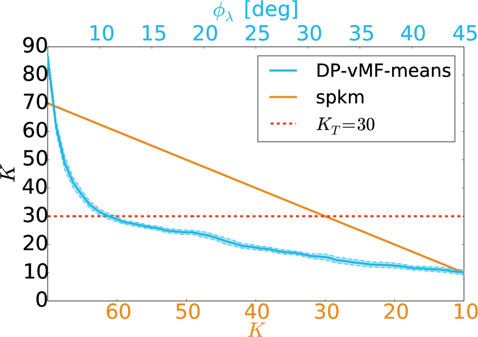
Synthetic Data: First, we evaluate the behavior of the DP-vMF-means algorithm in comparison to its parametric cousin, the spkm algorithm, on synthetic 3D spherical data sampled from $K_{\text{T}}=30$ true vMF distributions. All evaluation results are shown as the mean and standard deviation over 50 runs. The left plot of Fig. 3 depicts the inferred number of clusters $K$ on the horizontal axis as a function of the respective parameters of the two algorithms: the number of clusters $K$ for spkm and the parameter $\phi_{\lambda}$ for DP-vMF-means (recall that $\phi_{\lambda}=\cos^{-1}(\lambda+1)$ as defined in Sec. 4.1). This figure demonstrates the ability of the DP-vMF-means algorithm to discover the correct number of clusters $K_{\text{T}}$, and the relative insensitivity of the discovered number of clusters with respect to its parameter $\phi_{\lambda}$.

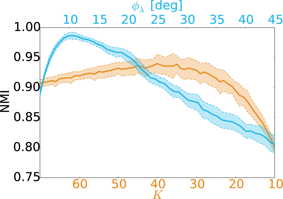
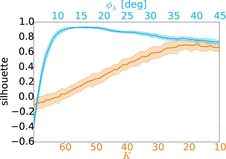
The middle and right hand plots show two measures for clustering quality. The normalized Mutual Information (NMI) [40], depicted in the middle, is computed using the true labels. DP-vMF-means achieves an almost perfect NMI of $0.99$, while spkm only reaches $0.94$ NMI even with $K=K_{\text{T}}$. The slightly superior performance of DP-vMF-means stems from its enhanced ability to avoid local optima due to the way labels are initialized: while spkm is forced to initialize $K$ cluster parameters, DP-vMF-means starts with an empty set and adds clusters on the fly as more data are labelled. The NMI results are corroborated by the silhouette score [36], shown to the right in Fig. 3. The silhouette score is an internal measure for clustering quality that can be computed without knowledge of the true clustering, and is used to tune parametric clustering algorithms. With a maximum of $0.92$ DP-vMF-means reaches a close to perfect silhouette score, indicating well-separated, concentrated clusters. Again, spkm does not reach the same clustering performance even for $K=K_{\text{T}}$ for the same aforementioned reasons.

Figure 6: Clustering of a surface normal stream recorded when walking a $90^{\circ}$ turn in an office environment. We depict key-frames color-coded with the implied surface-normal clustering for three clustering algorithms. The plots in the second and third row depict the percentage of normals associated to the respective cluster for DDP-vMF-means and sequential DP-vMF-means. Note that only the clustering obtained via the DDP-vMF-means algorithm is consistent across the whole run.

For additional reference we ran two sampling-based inference algorithms for the DP-vMF-MM model. The CRP-based inference of [4] was aborted after running for two days without convergence. This inefficiency has been noted previously [23]. A more efficient alternative is the finite Dirichlet process (FSD) approximation [22] to the DP-vMF-MM. The inference can be parallelized and yielded results within minutes. After $5000$ iterations the sampler converged to an incorrect number of $23.0\pm 1.67$ clusters on average over 10 sampler runs. These convergence issues have also been noted before [9]. The last sample of the different runs achieves an average NMI of $0.94\pm 0.01$ and a silhouette score of $0.74\pm 0.04$.

NYU v2 depth dataset: In this experiment, the DP-vMF-means and spkm algorithms were compared on the NYU v2 RGB-D dataset [31]. Surface normals were extracted from the depth images [19] and preprocessed with total variation smoothing [35]. We quantify the clustering quality in terms of the average silhouette score over the clusterings of the 1449 scenes of the NYU v2 depth dataset. Since we do not possess the true scene labeling, we use the silhouette quality metric as a proxy for the NMI metric; this was motivated by results of the synthetic experiment.

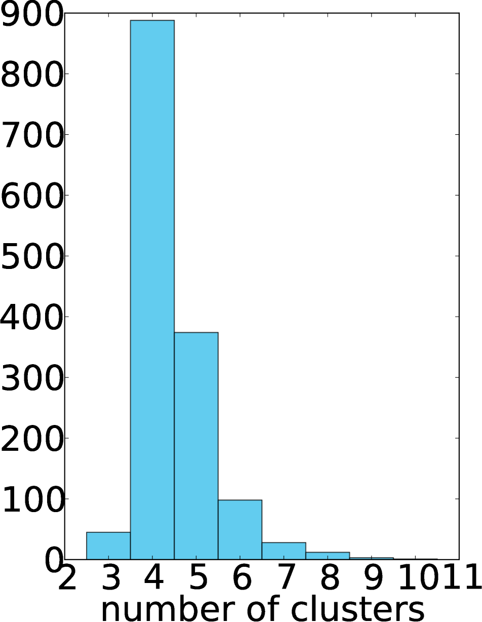
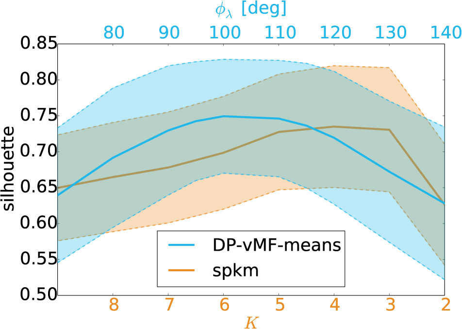
Across the whole NYU v2 dataset, the DP-vMF-means algorithm achieves the highest average silhouette score of $0.75$ for $\phi_{\lambda}^{\star}=100^{\circ}$ as depicted in Fig. 4. The histogram over the number of inferred clusters by DP-vMF-means for $\phi_{\lambda}^{\star}$ indicates the varying complexity of the scenes ranging from three to eleven. The clear peak at $K=4$ coincides with the highest silhouette score for spkm ($0.73$) and explains the only slightly lower silhouette score of spkm: most scenes in the dataset exhibit four primary directions.

Figure 5 shows a qualitative comparison of the scene segmentation implied by the clustering of surface normals. In comparison to spkm, the DP-vMF-means clustering results show the ability of the algorithm to adapt the number of clusters to the scene at hand. If the right number of clusters is selected for the spkm clustering, the results have similar quality; however, the number of clusters is generally not known a priori and varies across scenes. This demonstrates two major advantages of DP-vMF-means over spkm: (1) DP-vMF-means is less sensitive to the parameter setting (see Fig, 3, left) and (2) it is easier to choose $\phi_{\lambda}$ than $K$ since it intuitively corresponds to the maximum angular radius of a cluster, which can be gauged from the type of data and its noise characteristics. For this experiment $\phi_{\lambda}=100^{\circ}$ is justified by the typical Manhattan structure [10] of the indoor environment plus $10^{\circ}$ to account for sensor noise.

7.2 Evaluation of the DDP-vMF-means Algorithm

Real-time Directional Segmentation:

In fields such as mobile robotics or augmented reality, it is uncommon to observe just a single RGB-D frame of a scene; more typically, the sensor will observe a temporal sequence of frames. The following experiment demonstrates the temporally consistent clustering capability of the DDP-vMF-means algorithm on surface normals extracted from a sequence of depth images recorded in an indoor environment. Each frame is preprocessed in $11$ms using edge-preserving smoothing with a hybrid CPU-GPU guided filter [18].

We compare against the ad-hoc approaches of clustering on a frame-by-frame basis using DP-vMF-means, both with and without initializing the algorithm from the previous frame’s clusters. The former is referred to as sequential DP-vMF-means (sDP-vMF-means). sDP-vMF-means achieves a greedy frame-to-frame label consistency, but, unlike DDP-vMF-means, it cannot reinstantiate previous clusters after multiframe lapses. Motivated by the DP-vMF-means evaluation, all algorithms were run with $\phi_{\lambda}=100^{\circ}$. For DDP-vMF-means $\beta=10^{5}$ and $Q=\frac{\lambda}{400}$.

The differences in labeling consistency can be observed in rows two and three of Fig. 6, which shows the percentage of normals associated with a specific cluster. While DDP-vMF-means is temporally consistent and reinstantiates the lime-green and red clusters, observed in the first half of the run, DP-vMF-means erroneously creates new clusters. We do not depict the percentages of surface normals associated with the clusters for the batch DP-vMF-means algorithm, since the there is no label consistency between time-steps as can be observed in the last row of Fig. 6.

The average run-time per frame was $28.4$ ms for batch DP-vMF-means, $12.8$ ms for sDP-vMF-means, $20.4$ ms for DDP-vMF-means, and $13.6$ ms for spkm with $K=5$. The increased running time of batch DP-vMF-means is a result of clustering each batch of surface normals in isolation; OIR label assignment needs several restarts to assign labels to all surface normals. By initializing the clusters from a previous frame, sDP-vMF-means only incurs labeling restarts if a new cluster is observed, and hence has significantly lower run time. DDP-vMF-means is slightly slower than sDP-vMF-means since it is keeping track of both observed and unobserved clusters.

8 Conclusion

Taking the small-variance asymptotic limit of the Bayesian nonparametric DP-vMF and DDP-vMF mixture models, we have derived two novel spherical kmeans-like algorithms for efficient batch and streaming clustering on the unit hypersphere. The performance and flexibility of DP-vMF-means was demonstrated on both synthetic data and the NYU v2 RGB-D dataset. For DDP-vMF-means, Optimistic Iterated Restarts (OIR) parallelized label assignments, enable real-time temorally consistent clustering of batches of 300k surface normals collected at 30 Hz from a RGB-D camera.

We envision a large number of potential applications for the presented algorithms in computer vision and in other realms where directional data is encountered. Implementations are available at http://people.csail.mit.edu/jstraub/.

Acknowledgements

This work was partially supported by ONR MURI N00014-11-1-0688 and ARO MURI W911NF-11-1-0391.

References

- [1] M. Abramowitz and I. Stegun, editors. Handbook of Mathematical Functions. Dover Books on Mathematics. Dover Publications, 1965.
- [2] C. Antoniak. Mixtures of Dirichlet processes with applications to Bayesian nonparametric problems. The Annals of Statistics, 1974.
- [3] A. Banerjee, I. S. Dhillon, J. Ghosh, S. Sra, and G. Ridgeway. Clustering on the unit hypersphere using von Mises-Fisher distributions. JMLR, 6(9), 2005.
- [4] M. Bangert, P. Hennig, and U. Oelfke. Using an infinite von Mises-Fisher mixture model to cluster treatment beam directions in external radiation therapy. In ICMLA, 2010.
- [5] C. Bingham. An antipodally symmetric distribution on the sphere. The Annals of Statistics, 2(6):1201–1225, 1974.
- [6] D. Blackwell and J. B. MacQueen. Ferguson distributions via pólya urn schemes. The Annals of Statistics, 1973.
- [7] D. M. Blei, A. Y. Ng, and M. I. Jordan. Latent Dirichlet allocation. JMLR, 3:993–1022, 2003.
- [8] T. Campbell, M. Liu, B. Kulis, J. P. How, and L. Carin. Dynamic clustering via asymptotics of the dependent Dirichlet process mixture. In NIPS, 2013.
- [9] J. Chang and J. W. Fisher III. Parallel sampling of dp mixture models using sub-clusters splits. In NIPS, 2013.
- [10] J. M. Coughlan and A. L. Yuille. Manhattan world: Compass direction from a single image by Bayesian inference. In ICCV, 1999.
- [11] I. S. Dhillon and D. S. Modha. Concept decompositions for large sparse text data using clustering. Machine learning, 42(1-2):143–175, 2001.
- [12] M. P. do Carmo. Riemannian Geometry. Birkhäuser Verlag, Boston, MA, 1992.
- [13] T. Ferguson. A Bayesian analysis of some nonparametric problems. The Annals of Statistics, 1973.
- [14] N. I. Fisher. Statistical Analysis of Circular Data. Cambridge University Press, 1995.
- [15] Y. Furukawa, B. Curless, S. M. Seitz, and R. Szeliski. Manhattan-world stereo. In CVPR, 2009.
- [16] S. Gopal and Y. Yang. von Mises-Fisher clustering models. In ICML, 2014.
- [17] M. A. Hasnat, O. Alata, and A. Trémeau. Hierarchical 3-d von Mises-Fisher mixture model. In Workshop on Divergences and Divergence Learning, ICML, 2013.
- [18] K. He, J. Sun, and X. Tang. Guided image filtering. In ECCV, 2010.
- [19] D. Holz, S. Holzer, and R. B. Rusu. Real-Time Plane Segmentation using RGB-D Cameras. In Proceedings of the RoboCup Symposium, 2011.
- [20] B. K. P. Horn. Extended Gaussian images. Proceedings of the IEEE, 72(12):1671–1686, 1984.
- [21] K. Ikeuchi. Recognition of 3-d objects using the extended Gaussian image. In In IJCAI Conference, 1981.
- [22] H. Ishwaran and M. Zarepour. Exact and approximate sum representations for the Dirichlet process. Canadian Journal of Statistics, 30(2):269–283, 2002.
- [23] S. Jain and R. Neal. A split-merge Markov chain Monte Carlo procedure for the Dirichlet process mixture model. Journal of Computational and Graphical Statistics, 13:158–182, 2000.
- [24] K. Jiang, B. Kulis, and M. Jordan. Small-variance asymptotics for exponential family Dirichlet process mixture models. In NIPS, 2012.
- [25] J. T. Kent. The Fisher-Bingham distribution on the sphere. Journal of the Royal Statistical Society, pages 71–80, 1982.
- [26] B. Kulis and M. I. Jordan. Revisiting k-means: New algorithms via Bayesian nonparametrics. In ICML, 2012.
- [27] D. Lin, E. Grimson, and J. Fisher. Construction of dependent Dirichlet processes based on Poisson processes. NIPS, 2010.
- [28] S. N. MacEachern. Dependent nonparametric processes. In ASA Proceedings of the Section on Bayesian Statistical Science, 1999.
- [29] A. Makadia, A. Patterson, and K. Daniilidis. Fully automatic registration of 3D point clouds. In CVPR, 2006.
- [30] K. V. Mardia and P. E. Jupp. Directional statistics, volume 494. John Wiley & Sons, 2009.
- [31] P. K. Nathan Silberman, Derek Hoiem and R. Fergus. Indoor segmentation and support inference from RGBD images. In ECCV, 2012.
- [32] R. Neal. Markov chain sampling methods for Dirichlet process mixture models. Journal of Computational and Graphical Statistics, 9(2):249–265, 2000.
- [33] X. Pan, J. E. Gonzalez, S. Jegelka, T. Broderick, and M. Jordan. Optimistic concurrency control for distributed unsupervised learning. In NIPS, 2013.
- [34] J. Reisinger, A. Waters, B. Silverthorn, and R. J. Mooney. Spherical topic models. In ICML, 2010.
- [35] G. Rosman, Y. Wang, X.-C. Tai, R. Kimmel, and A. M. Bruckstein. Fast regularization of matrix-valued images. In ECCV, 2012.
- [36] P. J. Rousseeuw. Silhouettes: a graphical aid to the interpretation and validation of cluster analysis. Journal of Computational and Applied Mathematics, 20:53–65, 1987.
- [37] A. Roychowdhury, K. Jiang, and B. Kulis. Small-variance asymptotics for hidden Markov models. In NIPS, 2013.
- [38] J. Straub, J. Chang, O. Freifeld, and J. W. Fisher III. A Dirichlet process mixture model for spherical data. In AISTATS, 2015.
- [39] J. Straub, G. Rosman, O. Freifeld, J. J. Leonard, and J. W. Fisher III. A mixture of Manhattan frames: Beyond the Manhattan world. In CVPR, 2014.
- [40] A. Strehl and J. Ghosh. Cluster ensembles—a knowledge reuse framework for combining multiple partitions. JMLR, 3:583–617, 2003.
- [41] Y. W. Teh. Dirichlet processes. In Encyclopedia of Machine Learning. Springer, 2010.
- [42] R. Triebel, W. Burgard, and F. Dellaert. Using hierarchical EM to extract planes from 3D range scans. In ICRA, 2005.
- [43] S. Zhong. Efficient online spherical k-means clustering. In IJCNN, volume 5, pages 3180–3185. 2005.