Projected Equations of Motion Approach to Hybrid Quantum/Classical Dynamics in Dielectric-Metal Composites

Abstract

We introduce a hybrid method for dielectric-metal composites that describes the dynamics of the metallic system classically whilst retaining a quantum description of the dielectric. The time-dependent dipole moment of the classical system is mimicked by the introduction of projected equations of motion (PEOM) and the coupling between the two systems is achieved through an effective dipole-dipole interaction. To benchmark this method, we model a test system (semiconducting quantum dot-metal nanoparticle hybrid). We begin by examining the energy absorption rate, showing agreement between the PEOM method and the analytical rotating wave approximation (RWA) solution. We then investigate population inversion and show that the PEOM method provides an accurate model for the interaction under ultrashort pulse excitation where the traditional RWA breaks down.

I Introduction

The electronic structure and quantum dynamics of a system can be modelled using several approaches based on, e.g., wave function methods Landau and Lifshitz (1977), Green’s functions Stefanucci and van Leeuwen (2013); Nolting and Brewer (2009); Marini et al. (2009), density matrix theory Rand (2010); Boyd (2008) or density functional theory (DFT) Martin (2004); Marques et al. (2012). In practice, to model larger and larger electronic systems, high-performance computing facilities along with optimized algorithms are continually developed. To improve the scaling of the algorithm, hybrid approaches have been devised to break down the computational complexity of composite systems which include a small subsystem — still amenable of a fully quantum-mechanical treatment — and a larger environment — which is dealt with a lower level of approximation, most often classical. Examples of such composites include solvated molecules Cossi et al. (1996, 2002); Tomasi et al. (2005), protein-ligand interactions Murphy et al. (2000); Hensen et al. (2004); Gräter et al. (2005) and semiconductor-metal nanoparticle hybrids Lin et al. (2013); Singh (2013); Zhang et al. (2006); Artuso and Bryant (2010, 2012); Paspalakis et al. (2013); Kosionis et al. (2013); Cheng et al. (2007); Li et al. (2012); Singh (2013). In all these cases, we are more interested in the dynamics of the smaller subsystem and we look at the environment as a source of unavoidable perturbations.

Such hybrid approaches rely on the possibility to separate the composite system into two or more components whose dynamics are solved using different levels of approximation and to treat the residual interaction between the subsystems in an appropriate way. For example, a continuum solvation model (such as the polarizable continuum model) may be used in the solvated molecule problem where the molecule is treated using quantum mechanics (QM) and the solvent treated as a dielectric continuum, the interaction being electrostatic in nature Cossi et al. (1996, 2002); Tomasi et al. (2005); Corni et al. (2015). Various quantum mechanics/molecular mechanics (QM/MM) approaches have also been applied to model the protein-ligand interaction. In these cases, the ligand is treated using QM while the protein environment via MM and the potentials associated with the protein’s molecular make-up is approximated by means of classical force fields Murphy et al. (2000); Hensen et al. (2004); Gräter et al. (2005).

Hybrid methods have also been applied to model the coupling between molecules and metal nanoparticles (MNPs) upon optical excitation. For small MNPs, the composite system can still be treated fully quantum mechanically Zuloaga et al. (2009). For larger MNPs, classical electrodynamics is employed to model the MNP dynamics whereas a quantum description of the molecule is retained. In this case, the interaction between the MNP and the molecule is modeled through an effective electromagnetic coupling. These hybrid approaches make use of numerical methods such as the finite-difference time domain (FDTD) to solve the classical electrodynamics problem — namely, the Maxwell’s equations — while the dynamics of the molecular electrons are solved by means of time-dependent DFT. The overall dynamics are made self-consistent by including the electromagnetic field generated by the MNP into the molecular evolution and vice versa Chen et al. (2010); Coomar et al. (2011); Gao and Neuhauser (2013); Sakko et al. (2014).

In this work we propose an alternative, simpler and much less computationally expensive method that avoids the solution of Maxwell’s equations when the near–field effects in the electromagnetic coupling between the MNP and the quantum system (e.g., a molecule or a quantum dot) are negligible. To this end, we shall present a generalized model for treating the time-dependent interaction between a quantum system (QS) and classical system (CS) coupled through an electromagnetic field. The interaction is considered in the dipole-dipole approximation within the quasi-static limit. The dynamics of the QS are described via the density matrix master equation involving an effective field which depends on the time-dependent dipole moment of the CS. We note here that whilst we employ density matrix theory for the quantum dynamics, the method is general and can be applied to any time-dependent quantum mechanical approach such as those mentioned in the opening paragraph. The CS is modeled using classical electrodynamics in the linear response regime where the time-dependent dipole moment is reproduced by the introduction of a set of auxiliary degrees of freedom. These degrees of freedom enter into a set of projected equations of motion (PEOM) and are constrained by modeling the frequency-dependent polarizability of the CS.

As a testbed, we consider the hybrid system consisting of a semiconducting quantum dot (SQD) and MNP. In particular, the SQD is treated as an abstract two-level QS while the MNP is modelled as a gold nanosphere. This system has been studied extensively Zhang et al. (2006); Artuso and Bryant (2010, 2012); Paspalakis et al. (2013); Kosionis et al. (2013); Cheng et al. (2007); Li et al. (2012); Singh (2013) because it can be solved analytically by means of the rotating wave approximation (RWA). For continuous wave excitation, we show that this analytical benchmark for the energy absorption is correctly retrieved by the proposed hybrid approach. Pulsed excitations are also examined and agreement between the proposed method and the RWA approximation is shown if picosecond pulses are used. However, for a femtosecond pulse the RWA breaks down and an approach like the proposed method must be preferred.

The paper is organised as follows: In Section II, we describe the dipole-dipole interaction between the QS and CS and derive the PEOM method for treating the time-dependent dipole moment of the CS. The method is applied to a simple SQD-MNP system in Section III and the results for energy absorption rates and population inversion are compared with those from semi-analytical approximations. Finally, the conclusions are presented in Section IV.

II The PEOM Method

Figure 1: Schematic diagram showing the dipole-dipole interaction between a QS and a CS, separated by a distance $R$. When an external field, $\vec{E}_{\text{EXT}}$, is applied, a dipole, $\vec{P}_{\text{QS}}$, is induced in the QS thus generating a field. The CS thus experiences this dipole field in addition to the external field, and we denote the total field felt by the CS as $\vec{E}_{\text{CS}}$. Similarly, due to $\vec{E}_{\text{CS}}$, a dipole field is generated in the CS which is in turn felt by the QS in addition to $\vec{E}_{\text{EXT}}$, and we denote the total field felt by the QS as $\vec{E}_{\text{QS}}$. In this way, the QS and CS dynamics are coupled through the external field.

We consider a QS and a CS separated by a distance, $R$. An external field, $\vec{E}_{\text{EXT}}(t)$, is applied inducing a dipole-dipole interaction between the two systems (see Fig. 1). To simplify the notation, we assume that the QS and CS are isotropic media, though the method can be easily generalized to the anisotropic case. We write $\vec{E}_{\text{EXT}}(t)\equiv E_{\text{EXT}}(t)\hat{e}$ and denote the unit vector pointing along the line separating the centers of the particles as $\hat{n}$. The fields felt by the QS and CS are then, respectively Jackson (1962); Schmitt et al. (1999); Zhang et al. (2006),

$$\vec{E}_{\text{QS}}(t) =E_{\text{EXT}}(t)\hat{e}+\frac{P_{\text{CS}}(t)}{\epsilon_{\text{B}}R^{3}}\vec{g}\ ,$$ (1a)

$$\vec{E}_{\text{CS}}(t) =E_{\text{EXT}}(t)\hat{e}+\frac{P_{\text{QS}}(t)}{\epsilon_{\text{B}}R^{3}}\vec{g}\ ,$$ (1b)

where $P_{\text{CS}}(t)$ ($P_{\text{QS}}(t)$) is the total dipole moment of the CS (QS). $\epsilon_{\text{B}}$ is the dielectric constant of the background medium and

$$\vec{g}=3\hat{n}\left(\hat{e}\cdot\hat{n}\right)-\hat{e}\ .$$ (2)

The form of the fields here assumes only a dipole interaction. This is valid if $R$ is sufficiently large, but can be generalised to take into account higher multipole interactions as shown in Ref. Yan et al., 2008.

For demonstration, we shall presently use the density matrix approach to describe the quantum system, although the method is applicable to any time-dependent model. In the density matrix formalism, the dipole moment of the QS is given by

$$\vec{P}_{\text{QS}}(t)=\text{tr}\left(\bm{\rho}(t)\vec{\bm{\mu}}\right)\ ,$$ (3)

where $\text{tr}\left(\cdots\right)$ is the matrix trace operator, $\vec{\bm{\mu}}$ is the dipole moment operator matrix and $\bm{\rho}$ is the QS density matrix which evolves in time due to the field, $\vec{E}_{\text{QS}}(t)$, via the following master equation,

$$\dot{\bm{\rho}}=-\frac{i}{\hbar}\left[\bm{H}_{0},\bm{\rho}\right]+\frac{i}{\hbar}\vec{E}_{\text{QS}}(t)\cdot\left[\vec{\bm{\mu}},\bm{\rho}\right]+\eta\left(\bm{\rho}\right)\ .$$ (4)

In Eq. (4), $\bm{H}_{0}$ is the Hamiltonian of the unperturbed QS and the interaction energy with the time-dependent field $\vec{E}_{\text{QS}}(t)$ is treated within the electric dipole approximation (second term). $\eta\left(\bm{\rho}\right)$ is an additional function which can be used to model phenomenological effects not included in the Hamiltonian such as non-radiative decay (see Ref. Boyd, 2008, for example).

We assume that the CS has a frequency dependent polarizability $\alpha(\omega)$ which is known, e.g. by experiment or ab-initio calculations. Its dipole moment can then be described (in the linear response regime) via 

$$\vec{P}_{\text{CS}}(\omega)=\epsilon_{\text{B}}\alpha(\omega)\vec{E}_{\text{CS}}(\omega)\ .$$ (5)

In the time domain, the dipole moment is written in terms of the response function $\alpha(t)$,

$$\vec{P}_{\text{CS}}(t)=\epsilon_{\text{B}}\int_{-\infty}^{t}\alpha(t-t^{\prime})\vec{E}_{\text{CS}}(t^{\prime})dt^{\prime}\ .$$ (6)

Using a coupled iterative technique, we could then solve Eq. (4) numerically to obtain the time-dependent response of the QS to the effective field $\vec{E}_{\text{QS}}(t)$. However, computing the integral in Eq. (6) at each time-step in the solution is cumbersome and the values of $\vec{E}_{\text{CS}}(t)$ and $\alpha(t)$ for each time-step must be held in memory which may not be feasible for long simulations. This leads to the main component of the PEOM method, an alternative to calculating Eq. (6) directly by following a time-convolutionless scheme inspired by Ref. Stella et al., 2014.

We introduce $N$ complex auxiliary degrees of freedom, $\{s_{k}(t)\}$ for $k=1,2,\ldots,N$, which satisfy the following EOMs

$$\dot{\vec{s}}_{k}=-\left(\gamma_{k}+\text{i}\omega_{k}\right)\vec{s}_{k}+\text{i}\epsilon_{\text{B}}\vec{E}_{\text{CS}}(t)\ ,$$ (7)

and assume that $\vec{P}_{\text{CS}}(t)$ can be written as

$$\vec{P}_{\text{CS}}(t)=\sum_{k=1}^{N}c_{k}\vec{s}_{k}(t)\ ,$$ (8)

so that the memory-dependent integral in Eq. (6) is replaced with an expansion over the functions $\vec{s}_{k}$ found by solving the differential equations in Eq. (7). As these differential equations no longer contain a time-convolution (i.e., they are “memoryless”), they can be efficiently integrated by using standard iterative algorithms, e.g., the Runge-Kutta fourth-order method. All that is required is to find suitable values for the (real) parameters $\{c_{k},\gamma_{k},\omega_{k}\}$ in Eq. (7). The formal solution of Eq. (7) is

$$\vec{s}_{k}(t)=\epsilon_{\text{B}}\int_{-\infty}^{t}\text{i}\ e^{-\left(\gamma_{k}+\text{i}\omega_{k}\right)\left(t-t^{\prime}\right)}\vec{E}_{\text{CS}}(t^{\prime})dt^{\prime}\ .$$ (9)

Substituting the real part of Eq. (9) into Eq. (8) and rearranging yields

$$\vec{P}_{\text{CS}}(t)=\epsilon_{\text{B}} \int_{-\infty}^{t}\left(\sum_{k=1}^{N}c_{k}e^{-\gamma_{k}(t-t^{\prime})}\sin[\omega_{k}(t-t^{\prime})]\right)$$

$$\times\left(\vec{E}_{\text{CS}}(t^{\prime})\right)dt^{\prime}\ ,$$ (10)

and comparing with Eq. (6) we see that

$$\alpha(t)=\sum_{k=1}^{N}c_{k}e^{-\gamma_{k}t}\sin(\omega_{k}t)\ .$$ (11)

Then taking the Fourier transform of Eq. (11) (using the causality condition) gives

$$\alpha(\omega)=\sum_{k=1}^{N}\frac{c_{k}}{2}\left[\frac{1}{\omega+\omega_{k}+\text{i}\gamma_{k}}-\frac{1}{\omega-\omega_{k}+\text{i}\gamma_{k}}\right]\ .$$ (12)

Hence, the parameters $\{c_{k},\gamma_{k},\omega_{k}\}$ may be found by fitting the frequency-dependent polarizability of the CS (which is known) to the fitting functions on the RHS of Eq. (12) (e.g. using the least squares method as done in this work).

III The Quantum Dot-Metal Nanoparticle System

To test the PEOM method proposed in Sec. II, we use a semiconducting quantum dot (SQD) as the QS and a metal nanoparticle (MNP) as the CS since this hybrid system has been widely studied Zhang et al. (2006); Artuso and Bryant (2010, 2012); Paspalakis et al. (2013); Kosionis et al. (2013); Cheng et al. (2007); Li et al. (2012); Singh (2013) and some properties can be obtained analytically. In particular, we look at the energy absorption rate (EAR) and population inversion, which are associated with continuous and pulsed wave excitation respectively.

From Eq. (1), when an external field $E_{\text{EXT}}$ is applied, the fields felt by the SQD and MNP respectively are

$$E_{\text{SQD}} =E_{\text{EXT}}+g\frac{P_{\text{MNP}}}{\epsilon_{\text{B}}R^{3}}\ ,$$ (13)

$$E_{\text{MNP}} =E_{\text{EXT}}+g\frac{P_{\text{SQD}}}{\epsilon_{\text{B}}R^{3}}\ .$$ (14)

We have taken the external field to be polarized along the line connecting the centers of the particles, allowing us to drop the vector notation and set $g=2$ (see Eq. (2)).

The SQD is treated as a 2-level atomic system giving rise to a $2\times 2$ density matrix with elements that can be written as Boyd (2008); Zhang et al. (2006)

$$\begin{cases}\dot{\Delta}&=-\frac{4\tilde{\mu}_{21}}{\hbar}E_{\text{SQD}}(t)\text{Im}\left[\rho_{21}\right]-\Gamma_{11}(\Delta-1)\\ \dot{\rho}_{21}&=-\left(\Gamma_{21}+\text{i}\omega_{0}\right)\rho_{21}+\text{i}\frac{\tilde{\mu}_{21}}{\hbar}E_{\text{SQD}}(t)\Delta\end{cases}\ ,$$ (15)

where $\Delta(t)=\rho_{11}(t)-\rho_{22}(t)$ is the population difference between the ground and excited states with frequency difference $\omega_{0}$ which is known as the exciton frequency. $\Gamma_{11}$ and $\Gamma_{21}$ are the population decay and dephasing rates of the system respectively. The SQD is assumed to be a dielectric sphere with dielectric constant $\epsilon_{\text{S}}$ and so it has a screened dipole matrix element $\tilde{\mu}_{21}=\mu_{21}/\epsilon_{\text{effS}}$ where $\mu_{21}$ is the bare dipole matrix element and $\epsilon_{\text{effS}}=\frac{2\epsilon_{\text{B}}+\epsilon_{\text{S}}}{3\epsilon_{\text{B}}}$. Batygin et al. (1978)

For comparison with previous literature, the MNP is taken to be a gold sphere of radius $a$ and its polarizability is approximated by the Clausius-Mossotti formula,

$$\alpha_{\text{MNP}}(\omega)=a^{3}\frac{\epsilon_{\text{M}}(\omega)-\epsilon_{\text{B}}}{\epsilon_{\text{M}}(\omega)+2\epsilon_{\text{B}}}\ ,$$ (16)

where $\epsilon_{\text{M}}(\omega)$ is the frequency-dependent dielectric function of the bulk metal Landau et al. (1984) (we use the analytical model for bulk gold as given by Etchegoin et al. Etchegoin et al. (2006)). Note that there are no fundamental reasons for using an analytical expression for the polarizability. For example, $\alpha_{\text{MNP}}(\omega)$ may instead be extracted from experimental data or computed using a first-principles approach.

We take the SQD system parameters from Ref. Zhang et al., 2006. The dielectric constant is taken to be $\epsilon_{\text{S}}=6$ with transition dipole moment $\mu=0.65e$ nm and exciton energy $\hbar\omega_{0}=2.5$ eV close to the plasmon peak of the gold MNP. The decay and dephasing times are given by $\Gamma_{11}^{-1}=0.8$ ns and $\Gamma_{21}^{-1}=0.3$ ns. We assume the background medium is a vacuum so that $\epsilon_{\text{B}}=1$.

III.1 Energy Absorption Rate

We first look at the EAR of the hybrid system which is a steady-state property, found by considering the response to the following field,

$$E_{\text{EXT}}(t)=E_{0}\cos(\omega_{L}t).$$ (17)

In this case, Eq. (15) can be solved analytically within the RWA as shown in, e.g., Refs Zhang et al., 2006; Artuso and Bryant, 2010, 2012. In the RWA, the off-diagonal density matrix elements are first separated into slowly and quickly oscillating components,

$$\rho_{21}(t) =\bar{\rho}_{21}(t)e^{-\text{i}\omega_{L}t}\ ,$$ (18a)

$$\rho_{12}(t) =\bar{\rho}_{12}(t)e^{\text{i}\omega_{L}t}\ ,$$ (18b)

where $\bar{\rho}_{21}(t)$ and $\bar{\rho}_{12}(t)$ are assumed to vary on a much larger timescale than $2\pi/\omega_{L}$. The RWA assumes that $\omega_{L}\approx\omega_{0}$, neglecting terms oscillating at frequencies far from $\omega_{0}$, so that the following modified EOMS can be obtained from Eq. (15),

$$\begin{cases}\dot{\Delta}&=4\text{Im}\left[\left(\frac{\Omega_{\text{eff}}}{2}+G\bar{\rho}_{21}\right)\bar{\rho}_{12}\right]+\Gamma_{11}\left(1-\Delta\right)\\ \dot{\bar{\rho}}_{21}&=\left[\text{i}\left(\omega_{L}-\omega_{0}+G\Delta\right)-\Gamma_{21}\right]\bar{\rho}_{21}+\text{i}\frac{\Omega_{\text{eff}}}{2}\Delta\end{cases}\ ,$$ (19)

where

$$\Omega_{\text{eff}} =\Omega_{0}\left[1+\frac{g}{R^{3}}\alpha_{\text{MNP}}(\omega_{L})\right]\ ,$$ (20a)

$$G =\frac{g^{2}\tilde{\mu}_{21}^{2}}{\hbar\epsilon_{\text{B}}R^{6}}\alpha_{\text{MNP}}(\omega_{L})\ ,$$ (20b)

with $\Omega_{0}=\tilde{\mu}_{21}E_{0}/\hbar$ being the Rabi frequency of the isolated SQD.

The EAR of the SQD is defined as Artuso and Bryant (2010)

$$Q_{\text{SQD}}=\frac{1}{2}\hbar\omega_{0}\Gamma_{11}\left(1-\Delta^{\text{s.s.}}\right)\ ,$$ (21)

where $\Delta^{\text{s.s.}}$ is the value of $\Delta(t)$ when a steady-state has been reached, while the EAR of the MNP is Artuso and Bryant (2010)

$$Q_{\text{MNP}}=\left\langle\int j\cdot E_{\text{MNP}}^{(\text{in})}\ dV\right\rangle\ ,$$ (22)

where $j=\frac{\partial}{\partial t}(P_{\text{MNP}}(t)/V)$ is the current density in the MNP which has volume $V$ and $E_{\text{MNP}}^{(\text{in})}$ is the field inside the MNP. Within the RWA, it can be shown that $Q_{\text{MNP}}$ depends on $\bar{\rho}_{21}^{\text{s.s.}}$, the steady state value of $\bar{\rho}_{21}(t)$ Artuso and Bryant (2010). The total EAR of the system is then $Q=Q_{\text{MNP}}+Q_{\text{SQD}}$. An analytical solution for $\Delta^{\text{s.s.}}$ and $\bar{\rho}_{21}^{\text{s.s.}}$ can be obtained by setting the L.H.S. of Eq. (19) equal to zero (see Ref. Zhang et al., 2006 for example).

As an alternative to the above RWA solution, we numerically solve the original EOMs in Eq. (15) using the PEOM method where $P_{\text{MNP}}(t)$, which appears in the expression for $E_{\text{SQD}}(t)$, is approximated using Eq. (7) and Eq. (8). The fitting parameters, $\{c_{k},\gamma_{k},\omega_{k}\}$, are obtained from a least-squares fit of $\alpha_{\text{MNP}}(\omega)$ to the model in Eq. (12) over the range 0-20 eV which required $N=12$ fitting functions for sufficient accuracy.

Fig. 2 shows the total EAR for the hybrid system as a function of the laser detuning (field intensity $I_{0}$=1 W/cm²) for various separation distances of the two particles. We can see the expected quenching of $Q$ and the red-shift of the hybrid exciton energy as the particles are brought together as described in Ref. Zhang et al., 2006. The analytical RWA solutions are shown in solid lines while the crosses are the results taken from the PEOM method. In this case, we see perfect agreement between the two methods due to the validity of the RWA for the case of a sinusoidal external field with frequency very close to resonance with the SQD exciton frequency. We now turn our attention to short-pulse excitation to demonstrate a case where the RWA cannot be used.

Figure 2: Energy absorption rate, $Q$, for a SQD-MNP system with separation distances $R=13$ nm (green), 15 nm (red), 20 nm (blue) and 80 nm (black). The solid lines represent the steady-state analytical solution in the RWA while the crosses are the results from the PEOM method.

III.2 Population Inversion and Breakdown of the RWA

Population inversion occurs when the SQD is excited from the ground state to the excited state so that $\rho_{11}=0$, $\rho_{22}=1$ and is associated with short laser pulses (see, for example, Ref. Stievater et al., 2001). We consider a pulsed external field given by

$$E_{\text{EXT}}(t)=E_{0}f(t)\cos(\omega_{L}t)\ ,$$ (23)

where $f(t)$ is a dimensionless pulse envelope. The pulse area for an isolated SQD is defined as

$$\theta=\Omega_{0}\int_{-\infty}^{\infty}f(t)dt\ ,$$ (24)

and it is known that population inversion occurs at the end of the pulse for $\theta=(2n+1)\pi$ ($n=0,1,2,\ldots$) Wang et al. (2005).

We shall use a hyperbolic secant envelope defined by

$$f(t)=\text{sech}\left(\frac{t-\tau_{0}}{\tau_{p}}\right)\ ,$$ (25)

where $\tau_{0}$ is the center of the pulse and $\tau_{p}$ characterizes the pulse width. We choose the central frequency, $\omega_{L}$, to be resonant with the exciton frequency, i.e. $\hbar\omega_{L}=\hbar\omega_{0}=2.5$ eV, and we describe the pulse shape in terms of the number of cycles, $n$, by defining the pulse duration as

$$T=\frac{4\pi}{\omega_{L}}n\ ,$$ (26)

and choosing

$$\tau_{0}=T/2\ ,\quad\tau_{p}=T/30\ .$$ (27)

In this way we ensure the maximum amplitude, $E_{0}$, is achieved at the center of the pulse and that the external field is sufficiently close to zero at $t=0$ and $t=T$ for the values of $E_{0}$ considered here.

For the sech pulse in Eq. (25), it can easily be shown from Eq. (24) that for an isolated SQD, $\theta=\pi\Omega_{0}\tau_{p}$ and then a pulse of given duration can be described in terms of the pulse area by choosing the following field amplitude,

$$E_{0}=\frac{\hbar\theta}{\pi\tilde{\mu}_{21}\tau_{p}}\ .$$ (28)

In Ref. Paspalakis et al., 2013 it was shown that the pulse area for an SQD when coupled to the MNP may be written approximately as $\theta=\pi|\Omega_{\text{eff}}|\tau_{p}$ so that Eq. (28) becomes

$$E_{0}=\hbar\theta\left(\pi\tilde{\mu}_{21}\tau_{p}\left|1+\frac{g}{R^{3}}\alpha_{\text{MNP}}(\omega_{L})\right|\right)^{-1}\ .$$ (29)

In particular, it was stated that for short pulses ($\tau_{p}\sim 0.1$ ps) with amplitude given by Eq. (29), the resulting dynamics should be independent of $R$ as the influence of the parameter $G$ (see Eq. (20b)) becomes weaker.

In previous studies relating to pulsed excitations in SQD-MNP systems, the time-scales have generally been limited to relatively long pulses. For example in Ref. Sadeghi, 2010, 2009, the external field is switched on over tens of nanoseconds while in Ref. Paspalakis et al., 2013; Antòn et al., 2012, picosecond pulses are used. In such cases, the population dynamics can be found by solving the RWA EOMs in Eq. (19) but replacing $\Omega_{\text{eff}}$ with the time-dependent form,

$$\Omega(t)=f(t)\Omega_{\text{eff}}\ ,$$ (30)

giving

$$\begin{cases}\dot{\Delta}&=4\text{Im}\left[\left(\frac{\Omega(t)}{2}+G\bar{\rho}_{21}\right)\bar{\rho}_{12}\right]+\Gamma_{11}\left(1-\Delta\right)\\ \dot{\bar{\rho}}_{21}&=\left[\text{i}\left(\omega_{L}-\omega_{0}+G\Delta\right)-\Gamma_{21}\right]\bar{\rho}_{21}+\text{i}\frac{\Omega(t)}{2}\Delta\end{cases}\ .$$ (31)

The use of the RWA and slowly-varying envelope approximations respectively imply that solutions to (31) are only valid if ${\bar{\rho}}_{21}(t)$ and $f(t)$ vary much more slowly than $2\pi/\omega_{L}$. Recalling that $\hbar\omega_{L}=2.5$ eV, we therefore require the pulse duration to be much greater than $\sim 2$ fs.

Indeed, it is known that the RWA is not reliable for ultrashort (femto- and subfemto-second) pulses. Meier et al. (2007); Ziolkowski et al. (1995); Yang et al. (2015) This is demonstrated in Fig. 3 where we compare the solution of the original EOMs in Eq. (15) with those of the modified RWA EOMs in Eq. (31), showing the excited state population dynamics for an isolated SQD ($R\rightarrow\infty$) interacting with a picosecond and femtosecond pulse of area $5\pi$ (according to Eq. (28)). Fig. 3 (a) shows $\rho_{22}(t)$ for a 1000-cycle pulse ($\tau_{p}\approx 0.11$ ps) and we can see that the RWA in this case provides an adequate description of the dynamics, with population inversion occurring at the end of the pulse as expected for a $5\pi$ pulse. The inset shows a magnified region in which we can see the effect of the RWA neglecting the quickly oscillating terms: however, in the picosecond time-scale, these effects have negligible influence on the overall dynamics. Fig. 3 (b) shows $\rho_{22}(t)$ for a 10-cycle pulse ($\tau_{p}\approx 1.1$ fs) where the pulse duration is of a comparable time-scale to $2\pi/\omega_{L}$. In this case, we can see that the quickly oscillating terms neglected in the RWA solution have a more significant effect on the overall dynamics: importantly, complete population inversion is not achieved at the end of the pulse, and there is a much more oscillatory behaviour.

Figure 3: Excited state population dynamics for an isolated SQD ($R\rightarrow\infty$) interacting with a sech pulse of area $5\pi$ according to Eq. (28). The solid red line is the numerical solution to the original EOMs in Eq. (15) while the dashed blue line is the solution to the modified RWA EOMs in Eq. (31). (a) Dynamics for a 1000-cycle pulse corresponding to $\tau_{p}\approx 0.11$ ps. (b) Dynamics for a 10-cycle pulse corresponding to $\tau_{p}\approx 1.1$ fs.

In Ref. Yang et al., 2015, a numerical solution to Eq. (15) for pulsed excitation in SQD-MNP systems beyond the RWA is proposed. In deriving Eq. (31), $E_{\text{SQD}}(t)$ is expressed by separating out the positive and negative frequency parts as

$$E_{\text{SQD}}(t)\approx\frac{\hbar}{\tilde{\mu}_{21}}\left[\left(\frac{\Omega(t)}{2}e^{-\text{i}\omega_{L}t}+G\rho_{21}(t)\right)+\text{c.c.}\right].$$ (32)

Instead of invoking the usual RWA to arrive at Eq. (31), Yang et al. numerically solve Eq. (15) using as $E_{\text{SQD}}(t)$ the field in Eq. (32) (we shall call this method the effective field method). However, in deriving Eq. (32), one must first separate out the slowly oscillating components of the off-diagonal density matrix elements as in Eq. (18) (see e.g. Ref. Artuso and Bryant (2010)) and the slowly-varying envelope approximation must also be used. Thus, while the quickly oscillating terms are included, improving over the RWA, the pulse duration must still be longer than $2\pi/\omega_{L}$. We shall presently demonstrate how these assumptions render this approach unreliable for few-cycle pulses when the interparticle distances are small.

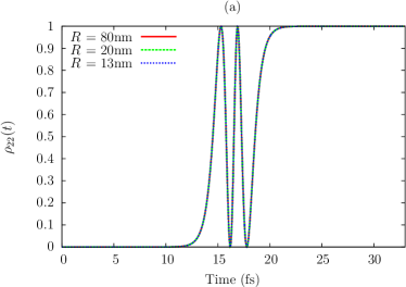
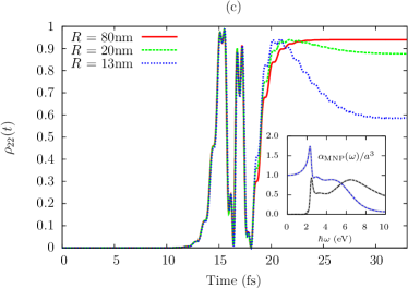
Figure 4: Excited state population dynamics for an SQD-MNP system interacting with a 10-cycle sech pulse for various interparticle distances, $R$. The field amplitude is chosen to give a $5\pi$ pulse area for each value of $R$ according to Eq. (29). (a) Solution to the modified EOMS in Eq. (31) under the RWA and assuming a slowly-varying pulse envelope. (b) Solution to the original EOMs in Eq. (15) beyond the RWA using the effective field in Eq. (32) which assumes a slowly-varying pulse envelope. (c) Solution to Eq. (15) using the PEOM method where the auxiliary parameters are obtained by fitting $\alpha_{\text{MNP}}(\omega)$ in Eq. (16) accurately over the range 0–10 eV using $N=21$ fitting functions. (d) Same as (c) but where $\alpha_{\text{MNP}}(\omega)$ is fitted over a small range close to $\hbar\omega_{0}$ (2.455–2.545 eV) using $N=1$ fitting functions. Insets: real (blue dashed) and imaginary (black dashed) parts of the fitted polarizability, $\alpha_{\text{MNP}}(\omega)/a^{3}$ (exact function shown in grey).

In Fig. 4, we compare the solutions for $\rho_{22}(t)$ based on the RWA, effective field method and the PEOM method. In each case, the SQD-MNP system interacts with a 10-cycle sech pulse of area $5\pi$ with $R$-dependent amplitude given by Eq. (29) and the excited state population dynamics are shown for various interparticle distances.

In Fig. 4 (a), the modified RWA EOMS in Eq. (19) are solved and we can see that complete population inversion occurs at the end of the pulse and the dynamics are identical for each $R$ as expected from Ref. Paspalakis et al., 2013 and Eq. (29).

In Fig. 4 (b), the original EOMS in Eq. (15) are solved beyond the RWA by taking $E_{\text{SQD}}(t)$ of the form in Eq. (32) similar to the calculations performed in Ref. Yang et al., 2015. In this case we see that the dynamics are almost identical to the isolated SQD as shown in Fig. 3 (b) where the original EOMs are solved exactly. At difference with the RWA solution in Fig. 4 (a), complete population inversion does not occur as a consequence of the RWA-breakdown. On the other hand, the dynamics remain independent of $R$ as predicted by Ref. Paspalakis et al., 2013. We note at this point that Ref. Paspalakis et al., 2013; Yang et al., 2015 employ a multipole description for the MNP response while our calculations use the simpler dipole model. However, we have compared results using the same multipole approximation and noticed no difference due to the short time-scales involved here.

In Fig. 4 (c), we solve the original EOMs in Eq. (15) using the PEOM method. We obtain the auxiliary parameters describing the MNP dipole moment by fitting $\alpha_{\text{MNP}}(\omega)$ in Eq. (16) to the functions in Eq. (12). This is achieved by a least-squares fit over the range 0–10 eV using $N=21$ fitting functions to gain a fit of sufficient accuracy (see inset). We see that for large $R$ ($R=80$ nm), $\rho_{22}(t)$ resembles the results in (b). However, as the interparticle distance decreases, the dynamics change considerably, with larger effect towards the end of the pulse. For each $R$, the dynamics are similar up to around 18 fs by which point the pulse is almost over (see Fig. 5 (b)). After this point, the population for each $R$ reaches the same maximum value (around 0.95), but at different times: $\sim 23$ fs for $R=80$ nm, $\sim 21$ fs for $R=20$ nm and $\sim 20$ fs for $R=13$ nm. The population then decreases more steeply as $R$ decreases, reaching as low as 0.6 for $R=13$ nm.

We ascribe the different results obtained with the PEOM in Fig. 4 (c) and the effective field method in Fig. 4 (b) to the fact that femtosecond pulses ($\sim 10$ cycles) excite a broad range of frequencies: in particular, much broader than the sub-picosecond pulses ($\sim 100$ cycles) for which the effective field method Yang et al. (2015) was originally developed. As stated earlier, in writing Eq. (32), $f(t)$ must be slowly varying and the off-diagonal density matrix elements must also first be separated into slowly and quickly oscillating components. These approximations indirectly force the MNP to respond only as $\alpha_{\text{MNP}}(\omega_{L})$ (i.e. only at the driving frequency), as apparent in the definitions of $\Omega_{\text{eff}}$ and $G$ in Eq. (20). However, the femtosecond pulse has a large bandwidth ($>1$ eV), thus exciting a broad range of frequencies in the MNP response. Moreover, $\alpha_{\text{MNP}}(\omega)$ changes significantly over this range close to $\hbar\omega_{0}=2.5$ eV due to the formation of the plasmon peak and thus one would expect the resulting time-dependent dipole moment, $P_{\text{MNP}}(t)$, (and therefore $E_{\text{SQD}}(t)$) to be modified compared with that for long pulses of smaller bandwidths. In Fig. 5, $P_{\text{MNP}}(t)$ is shown for the $R=13$ nm cases in Fig. 4 (b) and (c). We can see that in the effective field method, the MNP responds in phase with the external field, while in the PEOM method the dipole moment continues to propagate well after the pulse is over, thus contributing to the decline in population of the SQD.

Figure 5: Time evolution of the MNP dipole moment, $P_{\text{MNP}}(t)$, for the $R=13$ nm cases in Fig. 4 (b) (solid blue) and (c) (solid black) where the effective field method and PEOM method are used respectively. The corresponding external field is shown in dashed red.

Figure 6: Value of $\rho_{22}(t)$ at the end of the pulse for various pulse durations. The interparticle distance is $R=13$ nm and the pulse area is chosen to be $5\pi$ according to Eq. (29).

We have stated that in the effective field method, the MNP responds only at the driving frequency, $\omega_{L}$ (i.e. the polarizability is effectively constant, $\alpha_{\text{MNP}}(\omega)\approx\alpha_{\text{MNP}}(\omega_{L})$). This approximation is valid for monochromatic waves (e.g. Eq. (17)) and for long pulses. On the other hand, for very short pulses the frequency-dependence of the polarizability is important due to the larger bandwidth. The PEOM method overcomes this limitation as $\alpha_{\text{MNP}}(\omega)$ can be fitted over an arbitrary frequency range (as in Fig. 4 (c)) so that the relevant frequencies can be included in the dynamics. The constant polarizability of the effective field method can be simulated within the PEOM method by choosing a single, broad function ($N=1$) which agrees with $\alpha_{\text{MNP}}(\omega)$ at $\omega_{L}$ and is approximately constant over the pulse bandwidth region (see inset of Fig. 4 (d)). Fig. 4 (d) then shows that the effective field results from Fig. 4 (c) are indeed recovered.

Fig. 6 summarizes the results and shows the range of pulse durations for which the different approximations are valid. The three different methods agree for $n>100$ cycles ($\tau_{p}>10$ fs). The effective field method correctly describes the fall in final population as the pulse duration approaches 10 cycles due to the breakdown of the RWA, but we can see that when the full response of the MNP is taken into consideration in the PEOM method, the effect is much more enhanced.

Overall, the results of this section show that when examing the response of ultrashort pulses (fewer than $\sim 60$ cycles), one cannot rely on the RWA or on the assumption that the MNP polarizability ($\alpha_{\text{MNP}}$) responds only at the driving frequency, $\omega_{L}$. Therefore, one should consider more advanced approaches. The PEOM methods is a valid alternative as it is not bound by such approximations yet still its computational cost and complexity is similar to that of, e.g., the RWA or effective field method.

IV Conclusions

We have described a transferable hybrid approach to the electron dynamics of a quantum system dipolarly coupled to a larger environment that can be treated classically. This hybrid approach is based on a robust projected equations of motion (PEOM) formalism. The capabilities of the proposed hybrid approach have been demonstrated for the widely studied case of a semiconductor quantum dot (SQD) coupled to a metallic nanoparticle (MNP). The SQD has been modelled as a two-level system, while a semi-empirical model of the MNP susceptibility has been used. We have validated this hybrid approach against both analytical and semi-analytical benchmarks of the SQD-MNP response to picosecond laser pulses, i.e., longer than $2\pi/\omega_{0}$, where $\hbar\omega_{0}$ is the SQD energy gap. This is the regime of validity of the rotating wave approximation (RWA). However, the validity of the PEOM does not rely on either the RWA or improvements on it (e.g., the effective field methodYang et al. (2015)) and we have also modeled the response to femtosecond laser pulses. In this regime, we have shown that the response of the SQD-MNP is strongly affected by the details of the MNP susceptibility. By artificially “blurring” the details of the MNP susceptibility, the results of the hybrid approach match the prediction of the effective field method. To this extent, the proposed hybrid approach is inherently more accurate than the other methods which rely on the RWA and improvements on it.

Beyond the validation for a two-level system, the PEOM formalism can be used for systems with an arbitrary number of levels and is independent from the theoretical framework used to model the quantum system, e.g., the SQD. In this work, we have used a density matrix approach, but the PEOM can be easily formulated within a time-dependent density-functional theory framework, or the recently devised real-time approach to the Bethe-Salpeter equation Attaccalite et al. (2011) formalism.

The proposed hybrid approach shares similarities with other hybrid methods Coomar et al. (2011); Gao and Neuhauser (2013); Sakko et al. (2014) and, in principle, can be also coupled to a finite-difference time-domain (FDTD) description of the electromagnetic field. On the other hand, an accurate FDTD model is less crucial if the SQD and MNP are sufficiently far apart. Moreover, the simpler dipolar coupling used in this work is still popular Li et al. (2016); Terzis et al. (2016); Yang et al. (2015) and the PEOM formalism provides a necessary improvement as attention turns towards ultrafast phenomena.

When both the near-field response and the electromagnetic scattering can be safely neglected, the proposed hybrid method provides a computationally less expensive alternative to those more accurate approaches which include an FDTD model of the electromagnetic field. This hybrid approach is also easier to integrate into existing electronic structure codes, including codes which employ periodic-boundary conditions. This is particularly relevant for modelling extended quantum systems (e.g., two-dimensional semiconductors) coupled to MNPs. Eda and Maier (2013)