$\theta$ dependence of 4D $SU(N)$ gauge theories in the large-$N$ limit

Abstract

We study the large-$N$ scaling behavior of the $\theta$ dependence of the ground-state energy density $E(\theta)$ of four-dimensional (4D) $SU(N)$ gauge theories and two-dimensional (2D) $CP^{N-1}$ models, where $\theta$ is the parameter associated with the Lagrangian topological term. We consider its $\theta$ expansion around $\theta=0$, $E(\theta)-E(0)={1\over 2}\chi\,\theta^{2}(1+b_{2}\theta^{2}+b_{4}\theta^{4}+\cdots)$ where $\chi$ is the topological susceptibility and $b_{2n}$ are dimensionless coefficients. We focus on the first few coefficients $b_{2n}$, which parametrize the deviation from a simple Gaussian distribution of the topological charge at $\theta=0$.

We present a numerical analysis of Monte Carlo simulations of 4D $SU(N)$ lattice gauge theories for $N=3,\,4,\,6$ in the presence of an imaginary $\theta$ term. The results provide a robust evidence of the large-$N$ behavior predicted by standard large-$N$ scaling arguments, i.e. $b_{2n}=O(N^{-2n})$. In particular, we obtain $b_{2}=\bar{b}_{2}/N^{2}+O(1/N^{4})$ with $\bar{b}_{2}=-0.23(3)$. We also show that the large-$N$ scaling scenario applies to 2D $CP^{N-1}$ models as well, by an analytical computation of the leading large-$N$ $\theta$ dependence around $\theta=0$.

I Introduction

Some of the most intriguing properties of 4D $SU(N)$ gauge theories are those related to the dependence on the $\theta$ parameter associated with a topological term in the (Euclidean) Lagrangian

$$\mathcal{L}_{\theta}=\frac{1}{4}F_{\mu\nu}^{a}(x)F_{\mu\nu}^{a}(x)-i\theta q(x)\ ,$$ (1)

where $q(x)$ is the topological charge density,

$$q(x)=\frac{g^{2}}{64\pi^{2}}\epsilon_{\mu\nu\rho\sigma}F_{\mu\nu}^{a}(x)F_{\rho\sigma}^{a}(x)\ .$$ (2)

The dependence on $\theta$ vanishes perturbatively, therefore it is intrinsically nonperturbative book1 ; book2 ; book3 .

The recent renewed activity in the study of the topological properties of gauge field theories, and of $\theta$ dependence in particular, has been triggered by two different motivations. From the purely theoretical point of view $\theta$-related topics naturally appear in such disparate conceptual frameworks as the semiclassical methods Gross:1980br ; Schafer:1996wv ; Thomas:2011ee ; Unsal:2012zj ; Poppitz:2012nz ; Anber:2013sga ; Kharzeev:2015xsa , the expansion in the number of colors Witten:1980sp ; DiVecchia:1980ve ; Luscher:1978rn ; D'Adda:1978uc ; Witten:1978bc ; AA-80 ; Campostrini:1991kv ; CR-92 , the holographic approach Witten:1998uka ; Parnachev:2008fy ; Bigazzi:2014qsa ; Bigazzi:2015bna and the lattice discretization (see, e.g., Vicari:2008jw for a review of the main results). From the phenomenological point of view, the nontrivial $\theta$ dependence is related to the breaking of the axial $U_{A}(1)$ symmetry and related issues of the hadronic phenomenology Witten:1979vv ; Veneziano:1979ec ; Shore:2007yn , such as the $\eta^{\prime}$ mass. Moreover, it is related to the axion physics (see, e.g., Kim:2008hd for a recent review), put forward to provide a solution of the strong CP problem Peccei:1977hh ; Peccei:1977ur ; Wilczek:1977pj ; Weinberg:1977ma , i.e. to explain the fact that the experimental value of $\theta$ is compatible with zero, with a very small bound $|\theta|\lesssim 10^{-10}$ from neutron electric dipole measurements Baker:2006ts . Axions are also natural dark matter candidates Preskill:1982cy ; Abbott:1982af ; Dine:1982ah and, given the absence of SUSY signals from accelerator experiments, this is becoming one of the most theoretically appealing possibility.

The ground-state energy density of 4D $SU(N)$ gauge theories is an even function of $\theta$. It is expected to be analytic at $\theta=0$, thus it can be expanded in the form

$$E(\theta)-E(0)=\frac{1}{2}\chi\theta^{2}\big{(}1+b_{2}\theta^{2}+b_{4}\theta^{4}+\cdots\big{)}\ ,$$ (3)

where $\chi$ is the topological susceptibility, and the dimensionless coefficients $b_{2n}$ parametrize the non-quadratic part of the $\theta$ dependence. They are related to the cumulants of the topological charge distribution at $\theta=0$; in particular $b_{2n}$ quantify the deviations from a simple Gaussian distribution. Standard large-$N$ arguments predict the large-$N$ behavior Witten:1980sp ; Witten:1998uka ; Vicari:2008jw

$$\chi(N)=\bar{\chi}+O(N^{-2}),$$ (4)

$$b_{2n}(N)=\bar{b}_{2n}N^{-2n}+O(N^{-2n-2}).$$ (5)

Since $\chi$ and $b_{2n}$ can not be computed analytically, these large-$N$ scaling relations can be only tested numerically.

Earlier studies have mainly focused on the investigation of the large-$N$ scaling of the topological susceptibility, reporting a good agreement with the corresponding large-$N$ expectations (see, e.g., Lucini:2001ej ; DelDebbio:2002xa ; LTW-05 ). Instead, the numerical determination of the higher-order coefficients of the $\theta$ expansion turns out to be a difficult numerical challenge. Most efforts have been dedicated to the $SU(3)$ case DelDebbio:2002xa ; D'Elia:2003gr ; Giusti:2007tu ; Panagopoulos:2011rb ; Ce:2015qha ; Bonati:2015sqt , reaching a precision corresponding to a relative error below 10% only recently Bonati:2015sqt . Some higher-$N$ results were reported in Ref. DelDebbio:2002xa , presenting a first attempt to investigate the large-$N$ scaling of $b_{2}$; the numerical precision that could be reached was however quite limited, with a signal for $SU(4)$ at two standard deviation from zero and only an upper bound for $SU(6)$.

In order to further support the evidence of the large-$N$ scaling scenario beyond the quadratic term of the expansion of the ground-state energy dentity (3), we investigate the scaling of the higher-order terms, in particular those associated with $b_{2}$ and $b_{4}$. From the computational point of view, the most convenient method to perform such an investigation exploits Monte Carlo simulations of $SU(N)$ gauge theories in the presence of an imaginary $\theta$ angle, which are not plagued by the sign problem. Their analysis allows us to obtain accurate estimates of the coefficients of the expansion around $\theta=0$. Analogous methods based on computations at imaginary values of $\theta$ have been already employed in some numerical studies of the $SU(3)$ gauge theory aoki_1 ; Panagopoulos:2011rb ; D'Elia:2012vv ; D'Elia:2013eua ; Bonati:2015sqt and $CP^{N-1}$ models Azcoiti:2002vk ; Alles:2007br ; Alles:2014tta .

2D $CP^{N-1}$ models share with 4D $SU(N)$ gauge theories many physically interesting properties, like asymptotic freedom, dynamical mass generation, confinement, instantons and $\theta$ dependence; moreover their large-$N$ expansion can be studied by analytical methods Luscher:1978rn ; D'Adda:1978uc ; Witten:1978bc ; AA-80 ; Campostrini:1991kv ; CR-92 . As a consequence they are an attractive laboratory where to test theoretical ideas that might turn out to be applicable to QCD. An expansion of the form Eq. (3) applies also to the $\theta$ dependence of 2D $CP^{N-1}$ models. Similarly to 4D $SU(N)$ gauge theories, large-$N$ scaling arguments predict the large-$N$ behavior $\chi\approx c\,N^{-1}$ and $b_{2n}\approx\bar{b}_{2n}\,N^{-2n}$. These large-$N$ scaling behaviors are confirmed by explicit analytical computations, see Luscher:1978rn ; D'Adda:1978uc ; Witten:1978bc ; Campostrini:1991kv ; DelDebbio:2006yuf . In this paper, following the approach introduced in Rossi:2016uce , we present a systematic and easily automated way of computing the leading large-$N$ terms of $b_{2n}$.

The paper is organized as follows. In Section II we present the results obtained for the case of the 4D $SU(N)$ gauge theories: first we discuss the numerical setup used and the reasons for some specific algorithmic choices adopted, then we present the physical results obtained. In Section III the case of the 2D $CP^{N-1}$ models is discussed and a determination of the leading order large-$N$ expansion for the coefficients $b_{2n}$ is presented. Finally, in Section IV, we draw our conclusions. In appendices some technical details are examined regarding a comparison between smoothing algorithms in $SU(6)$ (App. A) and an attempt to reduce the autocorrelation time using a parallel tempering algorithm (App. B). Tables of numerical data are reported in App. C.

II Large $N$ in 4D $SU(N)$ gauge theories

II.1 Numerical setup

The traditional procedure that has been used in past to compute the coefficients entering Eq. (3) consists in relating them to the fluctuations of the topological charge $Q\equiv\int q(x)\mathrm{d}^{d}x$ at $\theta=0$. The first few coefficients of the expansion can indeed be written as (see e.g. Vicari:2008jw )

$$\chi=\frac{\langle Q^{2}\rangle_{\theta=0}}{\mathcal{V}},$$ (6)

$$b_{2}=-\frac{\langle Q^{4}\rangle_{\theta=0}-3\langle Q^{2}\rangle^{2}_{\theta=0}}{12\langle Q^{2}\rangle_{\theta=0}},$$ (7)

$$b_{4}=\frac{\left[\langle Q^{6}\rangle-15\langle Q^{2}\rangle\langle Q^{4}\rangle+30\langle Q^{2}\rangle^{3}\right]_{\theta=0}}{360\langle Q^{2}\rangle_{\theta=0}},$$ (8)

etc., where $\mathcal{V}$ is the 4D volume and all the averages are computed using the action with $\theta=0$. While this method is obviously correct from the theoretical point of view, it is numerically inefficient for the determination of the $b_{2n}$ coefficients. Indeed fluctuation observables are not self-averaging MBH and, in order to keep a constant signal to noise ratio, one has to dramatically increase the statistics of the simulations when increasing the volume (see e.g. Bonati:2015sqt for a numerical example). As a consequence it is extremely difficult to keep finite size effects under control and to extract the infinite-volume limit.

To avoid this problem, one can introduce a source term in the action, which allows us to better investigate the response of the system. This can be achieved by performing numerical simulations at imaginary values of the $\theta$ angle, $\theta\equiv-i\theta_{I}$, in order to maintain the positivity of the path integral measure and avoid a sign problem, and study for example the behaviour of $\langle Q\rangle_{\theta_{I}}$ as a function of $\theta_{I}$. It is indeed easy to verify that Panagopoulos:2011rb

$$\frac{\langle Q\rangle_{\theta_{I}}}{\mathcal{V}}=\chi\theta_{I}(1-2b_{2}\theta_{I}^{2}+3b_{4}\theta_{I}^{4}+\ldots)\ .$$ (9)

Also higher cumulants of the topological charge distribution (for which relations analogous to Eq. (9) exist) can be used for this purpose, however the numerical precision quickly degrades for higher cumulants. Nevertheless, since the computation of these higher cumulants does not require any additional CPU time, the optimal strategy seems to be to perform a common fit to a few of the lowest cumulants of the topological charge Bonati:2015sqt (of course by taking into account the correlation between them).

After this general introduction to motivate the computational strategy adopted, we describe the details of the discretization setup. For the $SU(3)$ case we use results already reported in the literature, while new simulations are performed for the $SU(4)$ and $SU(6)$ cases. The lattice action used in the sampling of the gauge configurations is

$$S[U]=S_{W}[U]-\theta_{L}Q_{L}[U]\,,$$ (10)

where $S_{W}[U]$ is the standard Wilson plaquette action Wilson:1974sk and $Q_{L}=\sum_{x}q_{L}(x)$. For the topological charge density we adopt the discretization DiVecchia:1981qi ; DiVecchia:1981hh :

$$q_{L}(x)=-\frac{1}{2^{9}\pi^{2}}\sum_{\mu\nu\rho\sigma=\pm 1}^{\pm 4}{\tilde{\epsilon}}_{\mu\nu\rho\sigma}\hbox{Tr}\left(\Pi_{\mu\nu}(x)\Pi_{\rho\sigma}(x)\right)\;,$$ (11)

where $\Pi_{\mu\nu}$ is the plaquette, $\tilde{\epsilon}_{\mu\nu\rho\sigma}$ coincides with the usual Levi-Civita tensor for positive entries and it is extended to negative ones by ${\tilde{\epsilon}}_{\mu\nu\rho\sigma}=-{\tilde{\epsilon}}_{(-\mu)\nu\rho\sigma}$ and complete antisymmetry. The discretization Eq. (11) of the topological charge density makes the total action in Eq. (10) linear in each gauge link, thus enabling the adoption of standard efficient update algorithms, like heat-bath and overrelaxation, a fact of paramount importance, since we have to deal with the strong critical slowing down of the topological modes DelDebbio:2002xa .

A practical complication is due to the fact that the discretization of the topological charge density induces a finite renormalization of $q(x)$ Campostrini:1988cy and thus of $\theta$. Denoting this renormalization constant by $Z$, we thus have

$$\theta_{I}=Z\theta_{L},$$ (12)

where $\theta_{L}$ is the numerical value that is used in the actual simulation. Two different strategies can be used to cope with this complication: in one case $Z$ is computed separately and Eq. (9) can then be directly used (see Panagopoulos:2011rb for more details). Another possibility consists in rewriting Eq. (9), and the analogous equations for the higher cumulants, directly in term of $\theta_{L}$, in such a way that by performing a common fit to the cumulants it is possible to evaluate both $Z$ and the parameters appearing in Eq. (3) (see Bonati:2015sqt for more details). In our numerical work we adopt the second strategy, that turn out to be slightly more efficient from the numerical point of view. All results that we present are obtained by analyzing the $\theta_{I}$ dependence of the first four cumulants of the topological charge distribution.

In order to avoid the appearance of further renormalization factors, the topological charge is measured on smoothed configurations. The smoothing procedure adopted uses the standard cooling technique Berg:1981nw ; Iwasaki:1983bv ; Itoh:1984pr ; Teper:1985rb ; Ilgenfritz:1985dz , which is the computationally cheapest procedure (especially for large values of $N$). Cooling is implemented à la Cabbibbo-Marinari, using the $N(N-1)/2$ diagonal $SU(2)$ subgroups of $SU(N)$, and we follow DelDebbio:2002xa in defining the measured topological charge $Q$ by

$$Q=\mathrm{round}\left(\alpha\,Q_{L}^{\rm smooth}\right)\ ,$$ (13)

where $\mathrm{round}(x)$ is the integer closest to $x$ and the coefficient $\alpha$ is the value that minimize

$$\left\langle\left(\alpha\,Q_{L}^{\rm smooth}-\mathrm{round}\left[\alpha\,Q_{L}^{\rm smooth}\right]\right)^{2}\right\rangle\ .$$ (14)

This procedure is introduced in order to avoid the necessity for prolongated cooling, and in fact we observe no significant differences in the results obtained by using a number of cooling steps between $5$ and $25$, while more than $100$ cooling steps would be needed to reach a plateau using just $Q_{L}$ instead of the $Q$ defined by Eq. (13). At finite lattice spacing, the two definitions (rounded vs. non-rounded) can lead to different results corresponding to different lattice artefacts, however it has been shown that the same continuum limit is reached in the two cases Bonati:2015sqt . The results that we present in the following are obtained using $15$ cooling steps and the definition of $Q$ in Eq. (13). We also mention that the results of this cooling procedure are compatible with those of other approaches proposed in the literature, see Vicari:2008jw ; Bonati:2014tqa ; Cichy:2014qta ; Namekawa:2015wua ; Alexandrou:2015yba and App. A.

Seven $\theta_{L}$ values are typically used in the simulations, going from $\theta_{L}=0$ to $\theta_{L}=12$ with steps $\Delta\theta_{L}=2$; when expressed in term of the renormalized parameter $\theta_{I}=Z\theta_{L}$ this range of $\theta_{L}$ values corresponds (for the couplings used in this work) to $\theta_{I}\lesssim 1.8$. We verify that this range of values is large enough to give a clear signal, but not so large to introduce systematic errors. The results of all tests performed using a smaller interval of $\theta_{L}$ values give perfectly compatible results.

For the update we use a combination of standard heat-bath Creutz:1980zw ; Kennedy:1985nu and overrelaxation Creutz:1987xi algorithms, implemented à la Cabibbo-Marinari Cabibbo:1982zn using all the $N(N-1)/2$ diagonal $SU(2)$ subgroups of $SU(N)$. The topological charge is evaluated every 10 update steps, one update step being composed of a heath-bath and five overrelaxation updates for all the links of the lattice, updated in a mixed checkerboard and lexicographic order. The total statistic acquired for each coupling value is typically of $O(10^{6})$ measures.

II.2 Numerical results

In order to apply the analytic continuation method in an actual computation, it is necessary to truncate the expansion in Eq. (9) (or, which is the same, in Eq. (3)) in order to fit the numerical data. We actually perform a global fit to the first four cumulants which, when rewritten in terms of $\theta_{L}$, read

$$\begin{split}\frac{\langle Q\rangle}{\mathcal{V}}&=\chi Z\theta_{L}(1-2b_{2}Z^{2}\theta_{L}^{2}+3b_{4}Z^{4}\theta_{L}^{4}+\dots)\,,\\ \frac{\langle Q^{2}\rangle_{c}}{\mathcal{V}}&=\chi(1-6b_{2}Z^{2}\theta_{L}^{2}+15b_{4}Z^{4}\theta_{L}^{4}+\dots)\,,\\ \frac{\langle Q^{3}\rangle_{c}}{\mathcal{V}}&=\chi(-12b_{2}Z\theta_{L}+60b_{4}Z^{3}\theta_{L}^{3}+\dots)\,,\\ \frac{\langle Q^{4}\rangle_{c}}{\mathcal{V}}&=\chi(-12b_{2}+180b_{4}Z^{2}\theta_{L}^{2}+\dots)\,.\end{split}$$ (15)

An example of such global fit, with a truncation including up to $O(\theta_{L}^{4})$ terms in the ground state energy density (i.e. setting $b_{4}=0$), is reported in Fig. 1 for the case of the $SU(4)$ gauge theory.

To quantify the systematic error associated with this procedure we consider two different truncations: in one case all the terms of Eq. (3) up to $O(\theta^{6})$ are retained (i.e. up to $b_{4}$), while in the other case a truncation up to $O(\theta^{4})$ (i.e. up to $b_{2}$) is used. Both truncations nicely fit the numerical data and the estimates of the coefficient $b_{4}$ turn out to be compatible with zero in all the cases. This is not surprising, since even for $SU(3)$ only upper bounds on $|b_{4}|$ exist (see, e.g., Panagopoulos:2011rb ; Bonati:2015sqt ) and its value is expected to approach zero very quickly as the number of colors is increased, see Eq. (4). We verify that the values of $Z,\chi$ and $b_{2}$ obtained by using the two different truncations are perfectly compatible with each other, indicating that no sizable systematic error is introduced by the truncation procedure, see the example in Fig. 2. For this reason we decide to use the $O(\theta^{4})$ truncation to estimate $Z$, $\chi$ and $b_{2}$, while the $O(\theta^{6})$ truncation is obviously needed to obtain an upper bound for $|b_{4}|$. Possible further systematic errors are checked by varying the fitted range of $\theta_{L}$ and verifying the stability of the fit parameters.

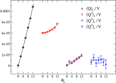
Figure 1: An example of the global fit procedure, with a truncation including $O(\theta_{L}^{4})$ terms: data refer to the $14^{4}$ lattice at coupling $\beta=11.008$ for the $SU(4)$ gauge theory. Continuous lines are the result of a combined fit of the first four cumulants.

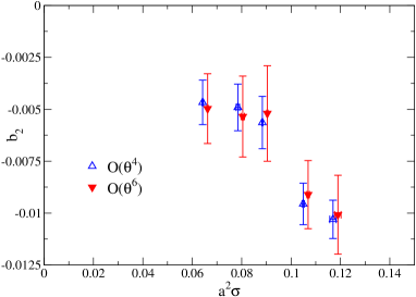
Figure 2: Comparison of the results obtained for $b_{2}$ in $SU(6)$ using different truncations of Eq. (3).

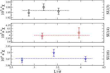
Figure 3: Dependence of $\chi$ (in lattice units) on the lattice size. From top to bottom results are displayed for: $SU(3)$ at coupling $\beta=6.2$ (from Bonati:2015sqt ), $SU(4)$ at $\beta=11.104$ and $SU(6)$ at $\beta=24.500$. Horizontal dashed lines are the results of fits to constant and are plotted in order to better appreciate the absence of statistically significant deviations.

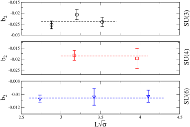
Figure 4: Dependence of $b_{2}$ on the lattice size. From top to bottom results are displayed for: $SU(3)$ at coupling $\beta=6.2$ (from Bonati:2015sqt ), $SU(4)$ at $\beta=11.104$ and $SU(6)$ at $\beta=24.500$. Horizontal dashed lines are the results of fits to constant and are plotted in order to better appreciate the absence of statistically significant deviations.

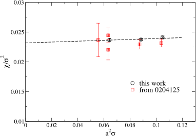
Figure 5: Continuum limit of the dimensionless ratio $\chi/\sigma^{2}$ for $SU(6)$ gauge theory. The results obtained in this work are compared with the determination of DelDebbio:2002xa (data have been slightly shifted horizontally to improve the readability).

$N$	$\quad\chi/\sigma^{2}$	$\qquad b_{2}$	$\qquad b_{4}$
3	0.0289(13)	$-$0.0216(15)	0.0001(3)
4	0.0248(8)	$-$0.0155(20)	$-$0.0003(3)
6	0.0230(8)	$-$0.0045(15)	$-$0.0001(7)

Table 1: Continuum extrapolated values for three, four and six colors. The value of $\chi/\sigma^{2}$ in $SU(3)$ was computed using data from Panagopoulos:2011rb , while for $b_{2n}$ we used the value reported in Bonati:2015sqt .

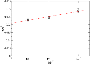
Figure 6: Scaling of the dimensionless ratio $\chi/\sigma^{2}$ with the number of colors. The dashed line is the result of a best fit with a linear functional dependence.

Hypercubic lattices of size $L\sqrt{\sigma}\gtrsim 3$ are used in all cases: they are expected to be large enough to provide the infinite-volume limit within the typical errors of our simulations (see e.g. DelDebbio:2002xa ). This is explicitly verified in some test cases: for example the $SU(6)$ simulations at coupling $\beta=24.500$ were replicated on lattices of size $L/a=8,10,12$ and for the coupling $\beta=24.845$ on lattices with $L/a=10,12,16$; in all cases no statistically significant volume dependence is observed, see Figs. 3-4. The possibility of using such large lattices in the determination of $b_{2}$ and higher cumulants is a consequence of the numerical setup adopted, with simulations performed at imaginary $\theta$ values.

Before starting to discuss our main subject, namely the determination of $b_{2}$ and its large $N$ behavior, we show that our data reproduce the well known large $N$ scaling of $\chi/\sigma^{2}$. For $SU(3)$ we use results already available in the literature (those reported in Tab. 1 of Panagopoulos:2011rb ) and for the scale setting in the $SU(4)$ and $SU(6)$ cases we used the determination of the string tension reported in DelDebbio:2001sj . For $SU(4)$ we observe no improvement with respect to the old results of DelDebbio:2002xa , since the final error on $\chi/\sigma^{2}$ is dominated by the error on the string tension. This is also the case for the final continuum result in the $SU(6)$ case, indeed we obtained $\chi/\sigma^{2}|_{SU(6)}=0.0230(8)$ to be compared with the value $0.0236(10)$ reported in Ref. DelDebbio:2002xa , however the continuum extrapolation of the new results is much more solid, as shown in Fig. 5.

The continuum values of $\chi/\sigma^{2}$ for $N=3,4$ and $6$ are reported in Tab. 1, their scaling with $N$ is shown in Fig. 6 and the result of a linear fit in $1/N^{2}$ gives

$$\chi/\sigma^{2}|_{SU(\infty)}=0.0209(11)\ ,$$ (16)

which slightly improves the previous result of Ref. Lucini:2001ej ; DelDebbio:2002xa ; LTW-05 ; Vicari:2008jw . Assuming the standard value $\sqrt{\sigma}=440$ Mev, we obtain $\chi_{SU(\infty)}^{1/4}=167(2)$ Mev. As noted before, the dominant source of error in $\chi/\sigma^{2}$ is the error on the string tension. As a consequence, to improve this result it would be enough to improve the precision of the $\sigma$ determination or to use different observables to set the scale. Since our main interest in this work is the analysis of the higher order cumulants $b_{2n}$, which are dimensionless, we have not pursued this investigation any further.

In Fig. 7 the results obtained for $b_{2}$ with $N=3,4,6$ are shown as a function of the (square of the) lattice spacing. The values of $a^{2}\sigma$ for the $SU(3)$ data have been computed using $r_{0}\sqrt{\sigma}=1.193(10)$ from Niedermayer:2000yx to plot the $b_{2}$ data from Bonati:2015sqt (where $r_{0}$ was used to set the scale) together with the new $SU(4)$ and $SU(6)$ data. For $SU(4)$, data are precise enough to perform a linear fit in $a^{2}\sigma$ and check for the systematics of the continuum extrapolation by varying the fit range; in particular the final error reported in Tab. 1 takes into account also fits obtained by excluding the data corresponding to the coarsest and to the finest lattice spacings. (for $SU(3)$ we use the value obtained in Bonati:2015sqt , where a similar analysis was performed). For the case of $SU(6)$ we could not reach lattice spacings as small as the ones used for $SU(3)$ and $SU(4)$ due to the dramatic increase of the autocorrelation times of the topological charge. To boost the sampling we tried using parallel tempering switches between different $\theta_{L}$ simulations but this did not result in a significant improvement (see App. B for more details). As a consequence, the analysis of the $SU(6)$ results can not be as statistically accurate as those for $SU(3)$ and $SU(4)$. In spite of this, a clear trend can be seen in the $SU(6)$ data shown in Fig. 7: $b_{2}$ flattens for $a^{2}\sigma\lesssim 0.1$, which is the region in which also $SU(4)$ data show no significant dependence on the lattice spacing, and we use the conservative estimate $b_{2}|_{SU(6)}=-0.0045(15)$, which is displayed in Fig. 7 by the horizontal blue dashed lines. For both $SU(4)$ and $SU(6)$ we increased significantly the precision of the $b_{2}$ determination with respect to results available in the literature: the previous estimates were indeed $b_{2}|_{SU(4)}=-0.013(7)$ and $b_{2}|_{SU(6)}=-0.01(2)$ from DelDebbio:2002xa , to be compared with the numbers reported in Tab. 1.

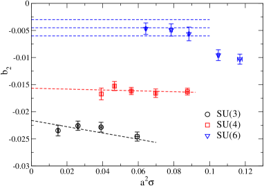
Figure 7: Dependence of the $b_{2}$ values on the lattice spacing for the case of three, four and six colors. See the main text for the details of the fitting procedure.

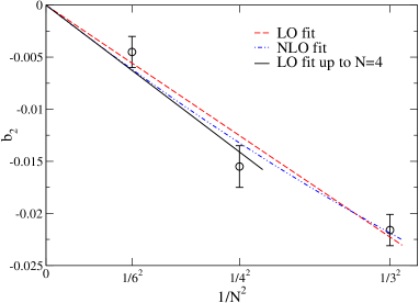
Figure 8: Scaling of $b_{2}$ with the number of colors. Lines are result of a best fit performed using the linear dependence expected from large $N$ arguments (dashed line fitting all data, full line fitting only those for $N=4,\,6$), and adding also a quadratic contribution (dotted-dashed line).

The estimates of $b_{2}$ versus the number of colors are shown in Fig. 8. They decrease with increasing $N$, strongly supporting a vanishing large-$N$ limit. Fitting the data to the Ansatz $b_{2}(N)=c/N^{\kappa}$ we obtain $\kappa=1.9(3)$, fully supporting the $1/N^{2}$ scaling predicted by the large-$N$ scaling arguments.

We now analyze the data assuming the $1/N^{2}$ scaling. Some fits are shown in Fig. 8. The leading form $b_{2}=\bar{b}_{2}/N^{2}$ of the expected $N$ dependence is used with two different fit ranges: in one case all the data are fitted, which gives $\bar{b}_{2}=-0.200(12)$ (with $\chi^{2}/\mathrm{dof}\sim 2.9/2$), while in the other case only data with $N>3$ are used, obtaining $\bar{b}_{2}=-0.23(3)$ (with $\chi^{2}/\mathrm{dof}\sim 1.9/1$). These results are in perfect agreement with those of the fit performed using also the NLO correction, i.e. to $b_{2}=\bar{b}_{2}/N^{2}+\bar{b}_{2}^{(1)}/N^{4}$, that gives $\bar{b}_{2}=-0.23(5)$ and $\bar{b}_{2}^{(1)}=0.3(5)$ (with $\chi^{2}/\mathrm{dof}\sim 2.5/1$), further indicating the absence of significant NLO correction. As our final estimate we report

$$\bar{b}_{2}=-0.23(3)\ .$$ (17)

The previous estimate for this quantity in the literature was $\bar{b}_{2}=-0.21(5)$ from DelDebbio:2002xa and it should be stressed that not only the error of the final result gets reduced in the present study, but also the whole analysis is now much more solid, since the old result relied heavily on the $SU(3)$ result.

Some estimates of the $O(\theta^{6})$ coefficient $b_{4}$ of the ground-state energy density are shown in Fig. 9. To extract a continuum value the same procedure adopted for $b_{2}$ was used also in this case: linear fits in $a^{2}$ were performed and consistency with the results obtained by discarding the values of the coarsest and the finest lattice spacings was verified. The final results are reported in Table 1. As previously anticipated, they are still compatible with zero. Assuming the large-$N$ scaling $b_{4}\simeq\bar{b}_{4}/N^{4}$ for $N=4$, we obtain the bound

$$|\bar{b}_{4}|\lesssim 0.1\ .$$ (18)

Our results for the large-$N$ coefficients $\bar{b}_{2n}$ may be compared with the analytical calculations by holographic approaches Witten:1998uka ; Parnachev:2008fy ; Bigazzi:2014qsa ; Bigazzi:2015bna . In particular, a compatible (negative sign) result for $\bar{b}_{2}$ is reported in Ref. Bigazzi:2015bna .

Finally in Fig. 10 we present our determinations of the renormalization factor $Z$ for $N=3,4$ and $6$ and for the various lattice spacings used (again $SU(3)$ data come from Bonati:2015sqt ). It can be noted that all the data approximately collapse on a common curve, i.e. $Z$ at fixed lattice spacing has a well defined large-$N$ limit. This behaviour could have been guessed by noting that the perturbative computation of $Z$ performed in Campostrini:1988cy is in fact (up to subleading corrections) an expansion in the ’t Hooft coupling $g^{2}N$.

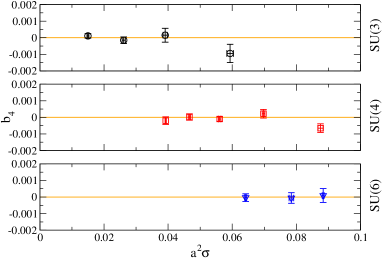
Figure 9: Estimates of $b_{4}$ for $N=3,\,4,\,6$.

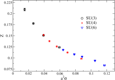
Figure 10: Dependence of the renormalization constant $Z$ values on the lattice spacing for the case of three, four and six colors.

III Large $N$ in 2D $CP^{N-1}$ models

The 2D $CP^{N-1}$ (Euclidean) Lagrangian in the presence of a $\theta$ term is:

$$\mathcal{L}_{\theta}(z,{\bar{z}})={N\over 2\,f}D_{\mu}{\bar{z}}D_{\mu}z+i{\theta\over 2\pi}\epsilon_{\mu\nu}\partial_{\mu}A_{\nu},$$ (19)

where $z$ is an $N$-component complex vector satisfying ${\bar{z}}\,z=1$, $D_{\mu}\equiv\partial_{\mu}+i\,A_{\mu}$ and $A_{\mu}\equiv i\,{\bar{z}}\,\partial_{\mu}z$. In order to analyze the large-$N$ behavior of the models one must introduce the Lagrange multiplier fields $\lambda_{\mu}$ and $\alpha$ and perform a Gaussian integration, thus obtaining the effective action

$$S_{\rm eff}(\lambda_{\mu},\alpha)= N\,{\rm Tr}\,\ln[-D_{\mu}D_{\mu}+i\,\alpha]-\frac{N}{2\,f}\int\mathrm{d}^{2}x\,[i\,\alpha]$$ (20)

$$-i\frac{\theta}{4\pi}\int\mathrm{d}^{2}x\,\,\epsilon_{\mu\nu}F_{\mu\nu}\ ,$$

where now $D_{\mu}\equiv\partial_{\mu}+i\,\lambda_{\mu}$ and $F_{\mu\nu}\equiv\partial_{\mu}\lambda_{\nu}-\partial_{\nu}\lambda_{\mu}$. The multiplier fields become dynamical and in particular $\lambda_{\mu}$ develops a massless pole, thus behaving as a bona fide (Abelian) gauge field.

The functional evaluation of $E(\theta)-E(0)$ in the large-$N$ limit can now be performed starting from the computation of the effective potential $N\,V(A,B)$ as a function of the constant vacuum expectation values $A(B)\equiv\langle i\,\alpha\rangle$ and $\langle F_{\mu\nu}\rangle=\epsilon_{\mu\nu}B$. In Ref Rossi:2016uce it has been shown that

$$V(A,B;\theta)=\frac{1}{4\,\pi}\Bigl{[} -A\,\ln\frac{2B}{m^{2}}-2B\,\ln\Gamma\left(\frac{1}{2}+\frac{A}{2B}\right)$$ (21)

$$+B\ln 2\pi-2\,i\,\frac{\theta}{N}\,B\Bigr{]}\ ,$$

where $m^{2}\equiv A(B\to 0)$ and $\Gamma$ is the standard Gamma function. It is now apparent that the natural expansion parameter for the large-$N$ evaluation of $E$ is $\bar{\theta}\equiv\theta/N$ Witten:1980sp ; Witten:1998uka .

To the purpose of evaluating $E(\theta)$ one must then solve the saddle point equations

$$\frac{\partial V}{\partial A}=0\ ,\qquad\frac{\partial V}{\partial B}=0\ .$$ (22)

The first equation may be employed in order to find the function $A(B^{2})$, independent of $\theta$, and to generate the large $N$ effective Lagrangian for the gauge degrees of freedom $V_{\lambda}(B;\theta)\equiv V[A(B^{2}),B;\theta]$.

The dependence on $\bar{\theta}$ of the large $N$ vacuum energy can now be found immediately from the relationship

$$E(\bar{\theta})-E(0)=N\,V_{\lambda}\bigl{[}B(\bar{\theta}),\bar{\theta}\bigr{]}\ ,$$ (23)

where $B(\bar{\theta})$ is the solution of the equation

$$\frac{\partial V_{\lambda}}{\partial B}=0\ .$$ (24)

One must appreciate that solving the last equation implies a continuation from real to complex values of $B$, that can be easily performed in the perturbative regime by observing that $V_{\lambda}(B;0)$ admits an asymptotic expansion in the even powers of $B$. Therefore it is possible to find a solution for purely imaginary $B$ in the form of a power series in the odd powers of $\bar{\theta}$.

The first few terms of the expansion of $B(\bar{\theta})$ are

$$B(\bar{\theta})\approx 6\,i\,m^{2}\,\bar{\theta}\bigl{(}1-{54\over 5}\bar{\theta}^{2}-{76014\over 175}\bar{\theta}^{4}+...\bigr{)},$$ (25)

where $m^{2}=A(\theta=0)$ is a square mass scale. Beside the leading large-$N$ behavior of the topological susceptibility D'Adda:1978uc ; Luscher:1978rn ; Witten:1978bc ; Campostrini:1991kv

$$\chi\approx{3m^{2}\over\pi N},$$ (26)

we obtain the rescaled coefficients $\bar{b}_{2n}\equiv{\rm lim}_{N\to\infty}N^{2n}b_{2n}$ of the $\theta$ expansion of the ground-state energy density:

$$\bar{b}_{2}=-{27\over 5},$$ (27)

$$\bar{b}_{4}=-\frac{25338}{175},$$

$$\bar{b}_{6}=-{16198389\over 875},$$

$$\bar{b}_{8}=-\frac{1500696182646}{336875},$$

etc… These results for $b_{2n}$ extend those reported in Ref. DelDebbio:2006yuf (in particular they correct the value of $\bar{b}_{4}$).

An analysis of several higher order coefficients shows that they are all negative and grow very rapidly, as one might have expected as a consequence of the nonanalytic dependence of the effective Lagrangian on $B$ already observed in Ref. Rossi:2016uce . In turn this phenomenon can be related to the fact that the full-fledged dependence on $\theta$ of the vacuum energy for any finite value of $N$ must exhibit a $2\pi$ periodicity which disappears in the large $N$ limit, thus implying a noncommutativity of the expansions and a vanishing radius of convergence in the variable $\bar{\theta}\equiv\theta/N$.

We finally mention that the large-$N$ behavior (26) of the topological susceptibility has been confirmed by numerical results of lattice $CP^{N-1}$ models CRV-92 ; V-92 ; ACDP-00 ; DMV-04 ; Vicari:2008jw . Instead, numerical results for the $\theta$-expansion coefficients $b_{2n}$ have never been obtained yet.

IV Conclusions

We study the large-$N$ scaling behavior of the $\theta$ dependence of 4D $SU(N)$ gauge theories and 2D $CP^{N-1}$ models, where $\theta$ is the parameter associated with the Lagrangian topological term. In particular, we focus on the first few coefficients $b_{2n}$ of the expansion (3) of their ground-state energy $E(\theta)$ beyond the quadratic approximation, which parametrize the deviations from a simple Gaussian distribution of the topological charge at $\theta=0$.

We present a numerical analysis of Monte Carlo simulations of 4D $SU(N)$ lattice gauge theories for $N=3,\,4,\,6$ in the presence of an imaginary $\theta$ term. This method, based on the analytic continuation of the $\theta$ dependence from imaginary to real $\theta$ values, allows us to significantly improve earlier determinations of the first few coefficients $b_{2n}$. The results provide a robust evidence of the large-$N$ behavior predicted by standard large-$N$ scaling arguments, i.e., $b_{2n}=O(N^{-2n})$. In particular, we obtain $b_{2}=\bar{b}_{2}/N^{2}+O(1/N^{4})$ with $\bar{b}_{2}=-0.23(3)$. The results for the next coefficient $b_{4}$ of the $\theta$ expansion (3) show that it is very small, in agreement with the large-$N$ prediction that $b_{4}=O(N^{-4})$. Assuming the large-$N$ scaling $b_{4}\approx\bar{b}_{4}/N^{4}$, we obtain the bound $|\bar{b}_{4}|\lesssim 0.1$.

An important issue concerns the consistency between the $\theta/N$ dependence in the large-$N$ limit and the $2\pi$ periodicity related to the topological phase-like nature of $\theta$. Indeed, the large-$N$ scaling behavior is apparently incompatible with the periodicity condition $E(\theta)=E(\theta+2\pi)$, which is a consequence of the quantization of the topological charge, as indicated by semiclassical arguments based on its geometrical meaning for continuous field configurations Gross:1980br . Indeed a regular function of $\bar{\theta}=\theta/N$ cannot be invariant for $\theta\to\theta+2\pi$, unless it is constant. A plausible way out Witten:1980sp is that the ground-state energy $E(\theta)$ tends to a multibranched function in the large-$N$ limit, such as

$$E(\theta)-E(0)=N^{2}\,{\rm Min}_{k}\,H\left({\theta+2\pi k\over N}\right),$$ (28)

where $H$ is a generic function. $E(\theta)$ is then periodic in $\theta$, but not regular everywhere. As a consequence, the physical relevance of the large-$N$ scaling of the $\theta$ dependence should be only restricted to the power-law expansion (3) around $\theta=0$, and of analogous expansions of other observables, thus to the $N$ dependence of their coefficients.

Our results significantly strengthen the evidence of the large-$N$ scaling scenario of the $\theta$ dependence, extending it beyond the $O(\theta^{2})$ expansion. We note that the large-$N$ scaling of the $\theta$ expansion is not guaranteed. Indeed there are some notable cases in which this does not apply. For example this occurs in the high-temperature regime of 4D $SU(N)$ gauge theories: for high temperatures the dilute instanton-gas approximation (DIGA) is expected to provide reliable results and one gets (see e.g. Gross:1980br ) the result $b_{2}=-1/12$ for any $N$ value. While the DIGA approximation is a priori expected to be valid only at asymptotically high temperatures, the switch from the large $N$ behavior to the instanton gas behavior occurs at the deconfinement transition temperature $T_{c}$ Bonati:2013tt .

The analytic continuation method that we used to compute the $\theta$ dependence can be also exploited in finite-temperature simulation, where it is typically even more efficient. As an example of its application in finite-temperature runs, Fig. 11 presents an updating of the results presented in Bonati:2013tt regarding the change of $\theta$ dependence across the deconfinement transition. While the results for $T>T_{c}$ were precise enough also in the original publication, the region below deconfinement is much more difficult (see the discussion in Bonati:2015sqt ). By combining the result for $SU(3)$ obtained in Bonati:2015sqt and the present ones for $SU(6)$, in the left side of Fig. 11 we can now display the continuum extrapolated zero temperature value of $b_{2}$ for $SU(6)$ and much more precise results for the finite temperature values of $b_{2}$. These results confirm the results of Bonati:2013tt to an higher accuracy: in the low-temperature phase the $\theta$-dependence properties, thus $\chi$ and $b_{2n}$, appear almost temperature independent, up to an abrupt change across the finite-temperature deconfinement transition. Then, in the high-temperature phase the $\theta$ dependence turns out to be that predicted by DIGA, with $b_{2n}$ not depending on $N$.

Finally, this paper also reports a study of the large-$N$ $\theta$ dependence of the 2D $CP^{N-1}$ models, whose leading behavior can be computed analytically. The results confirm the predicted large-$N$ scaling behavior $b_{2n}\approx\bar{b}_{2n}N^{-2n}$ for the coefficients of the expansion of the ground-state energy around $\theta=0$.

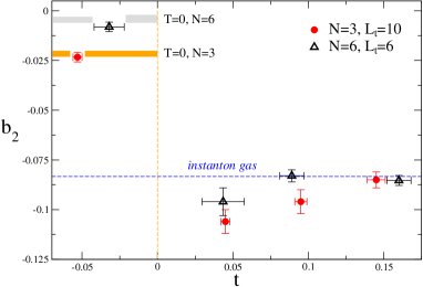
Figure 11: Behaviour of $b_{2}$ across the deconfinement transition for $SU(3)$ and $SU(6)$ ($t$ is the reduced temperature defined by $t=(T-T_{c})/T_{c}$). The horizontal bands denote the zero temperature values. Updated version of the figure originally presented in Bonati:2013tt .

Appendix A Cooling and gradient flow

It was shown in Bonati:2014tqa that cooling and the gradient flow with Wilson action give identical results for the topological charge when the number of cooling steps $n_{c}$ is related to the dimensionless flow time $\tau$ by the relation $n_{c}=3\tau$. This relation was explicitly verified by simulation in $SU(3)$ gauge theory and it was later extended to improved gauge actions Alexandrou:2015yba . During the early stages of this work we numerically verified on a subsample of configurations that, as theoretically expected, the same relation holds true also in the $SU(6)$ case. An example of the comparison between the two methods is reported in Fig. 12, which displays some generic features: in $SU(6)$ the topological charge is much more stable than in $SU(3)$, to reach a plateau of $Q_{L}$ around 100 cooling steps are needed, for very prolongated smoothing both cooling and gradient flow evolutions tunnel to the topologically trivial configuration and the tunneling typically happens first for the gradient flow.

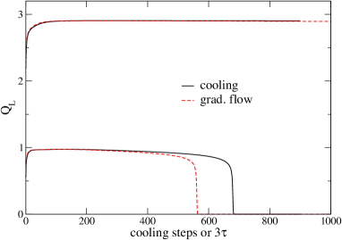
Figure 12: Comparison of cooling and gradient flow evolutions for two $SU(6)$ configurations.

Appendix B Parallel tempering in $\theta$

Parallel tempering Hukushima , also know as replica exchange Monte Carlo, is the most widely used variant of the simulated tempering algorithm Marinari:1992qd and was originally introduced to speed up simulations of spin glasses. In this appendix we report the results of some tests performed to investigate the effectiveness of parallel tempering to reduce the autocorrelation of the topological charge in $SU(6)$.

Parallel tempering is typically used in systems with complicated energy landscapes to reduce the autocorrelation times. The original idea is to perform standard simulations at various temperatures (with higher temperatures decorrelating faster than the lower ones) and once in a while try to exchange the configurations at different temperatures with a Metropolis-like step, that guarantees the detailed balance and hence the stochastic exactness of the algorithms. In this way the quickly decorrelating runs “feed” the slow ones and autocorrelations are drastically reduced.

For the case of gauge theories the first natural choice would be to use parallel tempering between runs at different $\beta$ values, with the runs at large values of $\beta$ playing the role of the slowly decorrelating ones. Although from a theoretical point of view this should work, one is faced with an efficiency problem: in order for the exchanges to be accepted with reasonable probability the $\beta$ values have to be close to each other, in fact closer and closer as the volume is increased, thus making the algorithm not convenient apart from extreme cases. See e.g. Ref. V-92 for applications to the 2D $CP^{N-1}$ models. This is the reason why alternative procedures have been proposed to work with different $\beta$ values, that are closer in spirit to the idea of multi-level simulations, see e.g. Endres:2015yca .

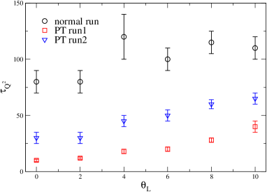
Figure 13: Autocorrelation times (in units of measure) of the square of the topological charge for the standard run and for the two tests with parallel tempering. In $run1$ an exchange was proposed every 4 measures, while in $run2$ it was proposed every 40 measures.

Since we are using simulations at nonvanishing values of the $\theta$ angle, an alternative possibility is to perform the switch step of the parallel tempering between runs at different $\theta_{L}$ values Panagopoulos:2011rb ; thetapt . In this case there are no “fast” and “slow” runs, but since the mean values of the topological charge are different for different $\theta_{L}$ values, the switch step characteristic of the parallel tempering is expected to effectively increase the tunneling rate of the topological charge.

As a testbed for the parallel tempering in $\theta_{L}$ we used $SU(6)$ with coupling $\beta=25.056$ and $\theta_{L}$ values from $-10$ to $10$ with $\Delta\theta_{L}=2$. Using the standard algorithm described in Sec. II.1 the autocorrelation time of the square of the topological charge is around $100$ measures (with 1 measure every 10 updates) and we tried two different exchange frequencies in the parallel tempering: in the run denoted by $run1$ an exchange was proposed every 4 measures, while in $run2$ it was proposed every 40 measures; in both the cases the proposed switch was accepted with a probability of about $70\%$.

$\beta$	$L/a$	$a\sqrt{\sigma}$	$\tau_{Q^{2}}$	$Z$	$a^{4}\chi$	$\chi/\sigma^{2}$	$b_{2}$	$b_{4}$
10.720	12	0.2959(14)	0.80(5)	0.09828(26)	$2.296(11)\times 10^{-4}$	0.02995(58)	-0.01628(62)	-0.00065(26)
10.816	12	0.2642(7)	1.6(1)	0.11231(49)	$1.4152(72)\times 10^{-4}$	0.02905(34)	-0.01658(79)	0.00022(26)
10.912	12	0.2368(6)	2.5(5)	0.12586(66)	$8.971(67)\times 10^{-5}$	0.02853(36)	-0.01617(67)	-0.00010(14)
11.008	14	0.2160(8)	6.0(5)	0.13792(88)	$6.044(48)\times 10^{-5}$	0.02776(47)	-0.01526(84)	0.00002(19)
11.104	16	0.1981(5)	14(1)	0.1518(14)	$4.129(62)\times 10^{-5}$	0.02681(48)	-0.0167(11)	-0.00020(23)

Table 2: $SU(4)$ data. String tension data from DelDebbio:2001sj . Autocorrelation times of the square of the topological charge are expressed in unit of measurements (one measure every 10 updates, see Sec. II.1 for more details on the update) and have been evaluated using the blocking method.

$\beta$	$L/a$	$a\sqrt{\sigma}$	$\tau_{Q^{2}}$	$Z$	$a^{4}\chi$	$\chi/\sigma^{2}$	$b_{2}$	$b_{4}$
24.500	12	0.3420(19)*	1.8(2)	0.08338(25)	$3.870(12)\times 10^{-4}$	0.02828(63)	-0.01030(92)	0.00008(60)
24.624	10	0.3239(8)	4.2(3)	0.09386(54)	$2.654(13)\times 10^{-4}$	0.02412(27)	-0.0096(10)	0.00011(31)
24.768	12	0.2973(5)	11(1)	0.10278(73)	$1.856(13)\times 10^{-4}$	0.02375(23)	-0.0056(13)	0.00009(42)
24.845	12	0.2801(13)*	22(3)	0.10832(78)	$1.545(11)\times 10^{-4}$	0.02509(50)	-0.0049(11)	-0.00006(32)
25.056	12	0.2534(6)	80(10)	0.11822(85)	$9.770(68)\times 10^{-5}$	0.02370(28)	-0.0047(10)	-0.00004(23)

Table 3: $SU(6)$ data. Most of the string tension data came from DelDebbio:2001sj , these denoted by * from Lucini:2003zr . Autocorrelation times of the square of the topological charge are expressed in unit of measurements (one measure every 10 updates, see Sec. II.1 for more details on the update) and have been evaluated using the blocking method.

The autocorrelation times of $Q^{2}$ for the different values of $\theta_{L}$ and the various run are shown in Fig. 13. As was to be expected given the range of $\theta_{L}$ used in the parallel tempering, small $\theta_{L}$ runs decorrelate faster than the ones with large $\theta_{L}$, and in all the cases an important decrease of $\tau_{Q^{2}}$ is observed, that is more significant for the case of $run1$, in which exchanges were proposed at higher rate than in $run2$. In the best case the autocorrelation time was reduced by around an order of magnitude with respect to the standard runs.

With respect to the single run at $\theta_{L}=0$ this reduction of $\tau_{Q^{2}}$ is however not sufficient to compensate for the CPU time required to perform the update of the 11 replicas used in the parallel tempering, since simulations at nonvanishing $\theta_{L}$ values are about 2.5 more time consuming than simulation at $\theta_{L}=0$.

On the other hand, the idea of the method of analytic continuation in $\theta$ for computing the $b_{2n}$ coefficients is exactly to use several $\theta_{L}$ values anyway, so that one can still hope to have an efficiency gain. This is however not the case: the simulations performed at different $\theta_{L}$ values are obviously correlated in the parallel tempering and, taking this correlation into account, no gain is apparently obtained by using the parallel tempering in the computation e.g. of $b_{2}$.

A possible explanation of this result (i.e. strong reduction of the autocorrelation for the single $\theta_{L}$ run and strong correlation between different $\theta_{L}$ runs) is the following. While on average the lattice operator $Q_{L}$ is obviously related to the operator $Q$, the specific form of their UV fluctuations can be different and are larger, in particular, for $Q_{L}$. As a consequence, the Metropolis test for the exchange of configurations, which is solely based on $Q_{L}$, could be easier, but then not accompained by a fast decorrelation of the global topological content $Q$ after the exchange, which would proceed with a decorrelation time likely comparable with the $\tau_{Q^{2}}$ of the standard simulation. If this interpretation is correct, then the observed reduction of the autocorrelation times at fixed $\theta_{L}$ is just a consequence of the reshuffling of the configurations induced by the exchanges, which are very frequent due to the largest UV fluctuations of $Q_{L}$. The update of the global information contained in the time histories at different $\theta_{L}$ values, which is the one used in the global fit, suffers instead from the usual autocorrelation problems.

One possibility, in order to improve the performance of the parallel tempering algorithm, could be to adopt an improved discretization of $Q_{L}$, e.g. a smeared definition of the topological charge density, such as those considered in Refs. CDPV-96 ; Laio:2015era ; this would require to abandon the heatbath and overrelaxation algorithms in favour of an Hybrid Monte Carlo approach Duane:1987de . However, it is not clear a priori whether that would result in an improvement of the global decorrelation properties, i.e. in a final net gain, or rather in a deterioration of the autocorrelation time for the single trajectory at fixed $\theta_{L}$, because of the rarer configuration reshuffling.

Appendix C Numerical data

In Tab. 2 and Tab. 3 we report the data obtained for $SU(4)$ and $SU(6)$ respectively at the different values of the coupling studied, together with the values of the string tension used in the analysis.

References

- (1) S. Coleman Aspects of symmetry, Cambridge University Press (1988).
- (2) A. Smilga Lectures on quantum chromodynamics, World Scientific (2001).
- (3) E. J. Weinberg Classical Solutions in Quantum Field Theory, Cambridge University Press (2012).
- (4) D. J. Gross, R. D. Pisarski and L. G. Yaffe, Rev. Mod. Phys. 53, 43 (1981).
- (5) T. Schäfer and E. V. Shuryak, Rev. Mod. Phys. 70, 323 (1998) [hep-ph/9610451].
- (6) E. Thomas and A. R. Zhitnitsky, Phys. Rev. D 85, 044039 (2012) [arXiv:1109.2608 [hep-th]].
- (7) M. Ünsal, Phys. Rev. D 86, 105012 (2012) [arXiv:1201.6426 [hep-th]].
- (8) E. Poppitz, T. Schäfer and M. Ünsal, JHEP 1303, 087 (2013) [arXiv:1212.1238].
- (9) M. M. Anber, Phys. Rev. D 88, 085003 (2013) [arXiv:1302.2641 [hep-th]].
- (10) D. E. Kharzeev and E. M. Levin, Phys. Rev. Lett. 114, 24, 242001 (2015) [arXiv:1501.04622 [hep-ph]].
- (11) E. Witten, Annals Phys. 128, 363 (1980).
- (12) P. Di Vecchia and G. Veneziano, Nucl. Phys. B 171 (1980) 253.
- (13) M. Luscher, Phys. Lett. B 78, 465 (1978).
- (14) A. D’Adda, M. Luscher, and P. Di Vecchia, Nucl. Phys. B 146, 63 (1978).
- (15) E. Witten, Nucl. Phys. B 149, 285 (1979).
- (16) I. Y. Arefeva and S. I. Azakov, Nucl. Phys. B 162, 298 (1980).
- (17) M. Campostrini and P. Rossi, Phys. Lett. B 272, 305 (1991).
- (18) M. Campostrini and P. Rossi, Phys. Rev. D 45, 618 (1992); Phys. Rev. D 46, 2741(E) (1992).
- (19) E. Witten, Phys. Rev. Lett. 81, 2862 (1998) [hep-th/9807109].
- (20) A. Parnachev and A. R. Zhitnitsky, Phys. Rev. D 78, 125002 (2008) [arXiv:0806.1736 [hep-ph]].
- (21) F. Bigazzi and A. L. Cotrone, JHEP 1501, 104 (2015) [arXiv:1410.2443 [hep-th]].
- (22) F. Bigazzi, A. L. Cotrone, and R. Sisca, JHEP 1508, 090 (2015) [arXiv:1506.03826 [hep-th]].
- (23) E. Vicari and H. Panagopoulos, Phys. Rept. 470, 93 (2009) [arXiv:0803.1593 [hep-th]].
- (24) E. Witten, Nucl. Phys. B 156, 269 (1979).
- (25) G. Veneziano, Nucl. Phys. B 159, 213 (1979).
- (26) G. M. Shore, Lect. Notes Phys. 737, 235 (2008) [hep-ph/0701171].
- (27) J. E. Kim and G. Carosi, Rev. Mod. Phys. 82, 557 (2010) [arXiv:0807.3125 [hep-ph]].
- (28) R. D. Peccei and H. R. Quinn, Phys. Rev. Lett. 38, 1440 (1977).
- (29) R. D. Peccei and H. R. Quinn, Phys. Rev. D 16, 1791 (1977).
- (30) F. Wilczek, Phys. Rev. Lett. 40 279 (1978).
- (31) S. Weinberg, Phys. Rev. Lett. 40 223 (1978).
- (32) C. A. Baker et al., Phys. Rev. Lett. 97, 131801 (2006) [hep-ex/0602020].
- (33) J. Preskill, M. B. Wise and F. Wilczek, Phys. Lett. B 120 127 (1983).
- (34) L. F. Abbott and P. Sikivie, Phys. Lett. B 120 133 (1983).
- (35) M. Dine and W. Fischler, Phys. Lett. B 120 137 (1983).
- (36) B. Lucini and M. Teper, JHEP 0106, 050 (2001) [hep-lat/0103027].
- (37) L. Del Debbio, H. Panagopoulos and E. Vicari, JHEP 0208, 044 (2002) [hep-th/0204125].
- (38) B. Lucini, M. Teper, and U. Wenger, Nucl. Phys. B 715, 461 (2005) [hep-lat/0401028].
- (39) M. D’Elia, Nucl. Phys. B 661, 139 (2003) [hep-lat/0302007].
- (40) L. Giusti, S. Petrarca and B. Taglienti, Phys. Rev. D 76, 094510 (2007) [arXiv:0705.2352 [hep-th]].
- (41) H. Panagopoulos and E. Vicari, JHEP 1111, 119 (2011) [arXiv:1109.6815 [hep-lat]].
- (42) M. Cé, C. Consonni, G. P. Engel and L. Giusti, Phys. Rev. D 92, 074502 (2015) [arXiv:1506.06052 [hep-lat]].
- (43) C. Bonati, M. D’Elia and A. Scapellato, Phys. Rev. D 93, 025028 (2016) [arXiv:1512.01544 [hep-lat]].
- (44) S. Aoki, R. Horsley, T. Izubuchi, Y. Nakamura, D. Pleiter, P. E. L. Rakow, G. Schierholz and J. Zanotti, arXiv:0808.1428 [hep-lat].
- (45) M. D’Elia and F. Negro, Phys. Rev. Lett. 109, 072001 (2012) [arXiv:1205.0538 [hep-lat]].
- (46) M. D’Elia and F. Negro, Phys. Rev. D 88, 034503 (2013) [arXiv:1306.2919 [hep-lat]].
- (47) V. Azcoiti, G. Di Carlo, A. Galante and V. Laliena, Phys. Rev. Lett. 89, 141601 (2002) [hep-lat/0203017].
- (48) B. Alles and A. Papa, Phys. Rev. D 77, 056008 (2008) [arXiv:0711.1496 [cond-mat.stat-mech]].
- (49) B. Alles, M. Giordano and A. Papa, Phys. Rev. B 90, 184421 (2014) [arXiv:1409.1704 [hep-lat]].
- (50) L. Del Debbio, G. M. Manca, H. Panagopoulos, A. Skouroupathis and E. Vicari, JHEP 0606, 005 (2006) [hep-th/0603041].
- (51) P. Rossi, Phys. Rev. D 94, 045013 (2016) [arXiv:1606.07252 [hep-th]].
- (52) A. Milchev, K. Binder and D. W. Heermann Z. Phys. B -Condensed Matter 63, 521 (1986).
- (53) K. G. Wilson, Phys. Rev. D 10, 2445 (1974).
- (54) P. Di Vecchia, K. Fabricius, G. C. Rossi and G. Veneziano, Nucl. Phys. B 192, 392 (1981).
- (55) P. Di Vecchia, K. Fabricius, G. C. Rossi and G. Veneziano, Phys. Lett. B 108, 323 (1982).
- (56) M. Campostrini, A. Di Giacomo and H. Panagopoulos, Phys. Lett. B 212, 206 (1988).
- (57) B. Berg, Phys. Lett. B 104, 475 (1981).
- (58) Y. Iwasaki and T. Yoshie, Phys. Lett. B 131, 159 (1983).
- (59) S. Itoh, Y. Iwasaki and T. Yoshie, Phys. Lett. B 147, 141 (1984).
- (60) M. Teper, Phys. Lett. B 162, 357 (1985).
- (61) E. M. Ilgenfritz, M. L. Laursen, G. Schierholz, M. Muller-Preussker and H. Schiller, Nucl. Phys. B 268, 693 (1986).
- (62) C. Bonati and M. D’Elia, Phys. Rev. D 89, 105005 (2014) [arXiv:1401.2441 [hep-lat]].
- (63) K. Cichy, A. Dromard, E. Garcia-Ramos, K. Ottnad, C. Urbach, M. Wagner, U. Wenger and F. Zimmermann, PoS LATTICE 2014, 075 (2014) [arXiv:1411.1205 [hep-lat]].
- (64) Y. Namekawa, PoS LATTICE 2014, 344 (2015) [arXiv:1501.06295 [hep-lat]].
- (65) C. Alexandrou, A. Athenodorou and K. Jansen, Phys. Rev. D 92, 125014 (2015) [arXiv:1509.04259 [hep-lat]].
- (66) M. Creutz, Phys. Rev. D 21, 2308 (1980).
- (67) A. D. Kennedy and B. J. Pendleton, Phys. Lett. B 156, 393 (1985).
- (68) M. Creutz, Phys. Rev. D 36, 515 (1987).
- (69) N. Cabibbo and E. Marinari, Phys. Lett. B 119, 387 (1982).
- (70) L. Del Debbio, H. Panagopoulos, P. Rossi and E. Vicari, JHEP 0201, 009 (2002) [hep-th/0111090].
- (71) B. Lucini, M. Teper and U. Wenger, JHEP 0401, 061 (2004) [hep-lat/0307017].
- (72) F. Niedermayer, P. Rufenacht and U. Wenger, Nucl. Phys. B 597, 413 (2001) [hep-lat/0007007].
- (73) M. Campostrini, P. Rossi and E. Vicari, Phys. Rev. D 46, 4643 (1992) [hep-lat/9207032].
- (74) E. Vicari, Phys. Lett. B 309, 139 (1993) [hep-lat/9209025].
- (75) B. Allés, L. Cosmai, M. D’Elia and A. Papa, Phys. Rev D 62, 094507 (2000) [hep-lat/0001027].
- (76) L. Del Debbio, G. Manca and E. Vicari, Phys. Lett. B 594, 315 (2004) [hep-lat/0403001].
- (77) C. Bonati, M. D’Elia, H. Panagopoulos and E. Vicari, Phys. Rev. Lett. 110, 252003 (2013) [arXiv:1301.7640 [hep-lat]].
- (78) K. Hukushima and K. Nemoto, J. Phys. Soc. Jpn. 65, 1604 (1996) [cond-mat/9512035].
- (79) E. Marinari and G. Parisi, Europhys. Lett. 19, 451 (1992) [hep-lat/9205018].
- (80) M. G. Endres, R. C. Brower, W. Detmold, K. Orginos and A. V. Pochinsky, Phys. Rev. D 92, 114516 (2015) [arXiv:1510.04675 [hep-lat]].
- (81) H. Panagopoulos and E. Vicari, (unpublished).
- (82) C. Christou, A. Di Giacomo, H. Panagopoulos, and E. Vicari, Phys. Rev. D 53, 2619 (1996) [hep-lat/9510023].
- (83) A. Laio, G. Martinelli and F. Sanfilippo, JHEP 1607, 089 (2016) [arXiv:1508.07270 [hep-lat]].
- (84) S. Duane, A. D. Kennedy, B. J. Pendleton and D. Roweth, Phys. Lett. B 195, 216 (1987).