QCD radiative corrections for in the Standard Model Dimension-6 EFT
Abstract
We calculate the QCD corrections to the inclusive decay rate in the dimension-6 Standard Model Effective Field Theory (SMEFT). The QCD corrections multiplying the dimension-6 Wilson coefficients which alter the -vertex at tree-level are proportional to the Standard Model (SM) ones, so next-to-leading order results can be obtained through a simple rescaling of the tree-level decay rate. On the other hand, contributions from the operators and , which alter the -vertex and introduce a -vertex respectively, enter at and induce sizeable corrections which are unrelated to the SM ones and cannot be anticipated through a renormalisation-group analysis. We present compact analytic results for these contributions, which we recommend to be included in future phenomenological studies.
I Introduction
The precise determination of the properties of the Higgs-like particle discovered during Run-I of the LHC Aad et al. (2012); Chatrchyan et al. (2012) is a main focus of the Run-II physics program. Within the current experimental precision, the coupling strengths of this particle appear to be consistent with the Standard Model (SM) Higgs boson Bolognesi et al. (2012); Aad et al. (2013, 2015a); Khachatryan et al. (2015); ATL (2015). With both theoretical and experimental developments, a significant improvement in the precision of the determination of the Higgs couplings is expected at the LHC during the High Luminosity (HL) phase Dawson et al. (2013).
The determination of the Higgs couplings which enter both production and decay processes is achieved by performing a (global) fit to data of the observable final states. This is necessary since a direct measurement of the SM Higgs boson width is not feasible at the LHC (or at proposed future colliders) since the expected value of MeV Andersen et al. (2013) is orders of magnitude smaller than the mass resolution of the detectors. The importance of a precision measurement of the partial width cannot be overstated, since this constitutes the dominant decay channel for the SM Higgs boson ( Andersen et al. (2013)). Consequently, a modification of the Higgs coupling to -quarks can have a sizeable impact on the extraction of all other Higgs couplings as the Higgs production rate and all branching fractions are modified by a shift in the total decay width .
Unfortunately, precision extractions of the partial and total width at the LHC are challenging. A measurement of the partial width is ultimately limited at the LHC, since knowledge of both the shape and normalisation of the contributing QCD backgrounds must be known to high accuracy Chatrchyan et al. (2014); Aad et al. (2015b). Current projections for a measurement of the signal strength indicate that precision may be achievable in the HL phase of the LHC Dawson et al. (2013). An extraction of the total width from experimental data (under minimal assumptions) through interference effects Dixon and Li (2013); Caola and Melnikov (2013); Campbell et al. (2014a, b, c) is possible, and additional information can also be gained by including LEP data Englert et al. (2016). However, the current constraint from this technique is approximately Khachatryan et al. (2014); Aad et al. (2015c). A precise model independent measurement of both these quantities requires input from a dedicated ‘Higgs machine’.
There are several design proposals for a collider with such capabilities, such as a linear/circular machine Aicheler et al. (2012); Behnke et al. (2013), muon-collider Alexahin et al. (2013); Delahaye et al. (2013), or machine Asner et al. (2003); Bogacz et al. (2012). Although the proposed physics programs are different in each case, the common goal is to achieve level precision on the measurement of Higgs couplings. For example, through a combination of a Higgs recoil measurement and an exclusive measurement of , better than 10% precision on the total width can be expected Baer et al. (2013). In the case of the branching fraction, better than precision is expected in some cases — see Table 2.3 of Baer et al. (2013). In such a scenario, precision calculations are also required to interpret the data. In this work, we focus on the QCD corrections to the Higgs decay to -quarks in the framework of the Standard Model Effective Field Theory (SMEFT).
In the SMEFT framework, the effects of physics beyond the SM are parameterised by a set of non-vanishing Wilson coefficients of higher-dimensional operators. Practically, the usual dimension-4 SM Lagrangian is extended to include operators of mass-dimension , which are constructed from gauge-invariant combinations of SM fields and multiplied by Wilson coefficients of mass dimension (). These operators effectively describe the interactions of new physics particles with those present in the SM, an approach which may be justified if the energy scale of these new particles greatly exceeds the electroweak scale. One of the main benefits of this approach is that new physics effects can be characterised without specifying a particular UV complete model of physics Beyond-the-SM (BSM). The interpretation of data in terms of non-vanishing Wilson coefficients is therefore performed in a model-independent fashion. In the absence of any direct evidence for new particle states during Run-I of the LHC, we believe this approach to be both justified and well motivated.
During Run-I, the interpretation of Higgs measurements by ATLAS and CMS was generally performed in the ‘interim’ and signal strength formalisms — see for example the combined Run-I analysis of CMS and ATLAS data ATL (2015). In Run-II, it is a recommendation of the LHC Higgs Cross Section Working Group to move towards a more general EFT framework (see for instance Section 10.4 of Andersen et al. (2013)). In doing so, it is important to note that the predictions for observables obtained in SMEFT are not unlike those obtained in the SM (or UV-completions of the SM for that matter) where a perturbative expansion has been applied — higher-order corrections reduce the theoretical uncertainty of the predictions of observables. Moreover, the next-to-leading order (NLO) corrections to a given observable typically depend on Wilson coefficients which are not present in the tree-level result. It is therefore important to extend SMEFT analyses to NLO (and beyond), to allow for a more precise determination of Wilson coefficients (and allowed ranges) through a comparison with experimental data, and much recent work has been dedicated to this task for a wide range of processes Elias-Miro et al. (2013a, b); Elias-Miro et al. (2014); Jenkins et al. (2013); Zhang and Maltoni (2013); Jenkins et al. (2014); Alonso et al. (2014); Passarino (2013); Chen et al. (2014); Grojean et al. (2013); Zhang (2014b); Englert and Spannowsky (2015); Zhang (2014a); Pruna and Signer (2014); Henning et al. (2014); Degrande et al. (2015); Buarque Franzosi and Zhang (2015); Ghezzi et al. (2015); David and Passarino (2015); Grober et al. (2015); Hartmann and Trott (2015a, b); Gauld et al. (2016); Zhang (2016); Bessidskaia Bylund et al. (2016); Gorbahn and Haisch (2016); Maltoni et al. (2016).
At present, it is possible to deduce logarithmically enhanced NLO corrections appearing in fixed-order perturbation theory to arbitrary observables using renormalisation-group (RG) equations for the Wilson coefficients along with the full one-loop anomalous dimension matrix calculated in Jenkins et al. (2013, 2014); Alonso et al. (2014). However, it is common practice to use RG-improved perturbation theory to absorb such logarithmic corrections into the running of the scale-dependent Wilson coefficients between and the scale at which the underlying decay or scattering process takes place (for decays this is ). This removes large logarithms involving from effective theory matrix elements, and allows constraints on Wilson coefficients obtained at experimentally accessible energy scales to be interpreted at the scale where the effective interactions are generated. The remaining NLO corrections do not contain large logarithms involving the scale , and cannot be deduced from an RG analysis. However, these corrections can still be important numerically because for the interesting region of TeV the RG-induced logarithms are not dramatically enhanced.
In this work, we extend our previous calculation of such NLO SMEFT corrections arising from four-fermion contributions and the (presumably) numerically dominant electroweak corrections Gauld et al. (2016) by computing the correction to the decay rate. We proceed by introducing the relevant details of the SMEFT framework for the decay, and discuss the renormalisation procedure we adopt for performing SMEFT NLO calculations. We then provide the analytic results, and make recommendations for their use in phenomenological studies.
II Calculational Set-up
II.1 Preliminaries
In the SMEFT, the usual SM Lagrangian is appended by higher-dimensional operators multiplied by Wilson coefficients. In the current work we are interested in dimension-6 operators, and so use a Lagrangian of the form
| (1) |
The operators relevant for this work are listed in Table 1. Note that in our convention the Wilson coefficients of dimension-6 operators have mass dimension minus two, so that the are suppressed by , and that we have rescaled the operator by a factor of the strong coupling constant with respect to the usual definition. The relevant interaction Lagrangian for Higgs couplings to down-type quarks is
| (2) |
where and are complex matrices in flavour space. The Higgs potential is also altered compared to the SM, and requiring that the kinetic terms are canonically normalised leads one to write the Higgs doublet in unitary gauge in the broken phase of the theory as
| (5) |
where
| (6) |
and the vacuum expectation value , with the Fermi constant. It should be noted that although is dimensionless, due to the presence of in its definition, it is still understood to be implicitly suppressed by .
Throughout this work, we are concerned with the flavour conserving process . However, the matrices and appearing in Eq. (II.1) are in general not simultaneously diagonalisable, leading to flavour violating effects which are not present in the SM. The running of also introduces further flavour violating effects which should be considered Alonso et al. (2014); Wells and Zhang (2015). We follow the procedure taken in previous work Gauld et al. (2016), imposing a minimal flavour violation (MFV) scenario Chivukula and Georgi (1987); D’Ambrosio et al. (2002) and setting throughout. The -quark Yukawa coupling, defined as the coefficient of the -vertex in the mass basis of the broken phase of the theory, is therefore related to the physical mass according to
| (7) |
With these preliminaries in place, it is straightforward to compute the tree-level amplitude for the process as
| (8) |
where
| (9) |
II.2 Renormalisation procedure
The calculation of the QCD corrections to in the SMEFT proceeds much the same way as in the SM. In addition to calculating the real and virtual contributions to the NLO matrix elements, which we discuss below, we must also construct a set of counterterms which render the virtual corrections UV finite. There is some subtlety in the construction of such UV counterterms, and we therefore provide details on the renormalisation procedure here111The reader is directed to a previous publication Gauld et al. (2016) for a more extensive discussion.. In essence, wavefunction and parameter/mass renormalisation is performed in the on-shell scheme, and Wilson coefficients are renormalised in the scheme.
We first discuss the calculation of the renormalisation constants for the external fields and parameters/masses. This proceeds as in the SM, and a detailed discussion of this procedure for the SM can be found in Denner (1993). While the full procedure including also electroweak corrections is rather involved, for the QCD corrections to we need only renormalise the -quark field and mass. We relate renormalised and bare quantities according to
| (10) |
where the superscript labels the bare field or mass. Explicit expressions for the one-loop renormalisation constants are obtained from the -quark two-point function. When computing the renormalisation constants, the divergences are regulated by performing the loop integrals in dimensions. The relevant one-loop renormalisation constants are found to be
| (11) |
where is the number of colours in QCD, , and
| (12) |
The SM and dimension-6 contributions are distinguished through the superscript and respectively. It is worth noting that we follow the convention of Kniehl and Pilaftsis (1996) by requiring to be real.
We must also include counterterms related to operator renormalisation. These counterterms are generated from the operators whose Wilson coefficients appear in the tree-level expression in Eq. (9), and are in fact simple to construct using that expression as a starting point. We do this by interpreting those as bare Wilson coefficients, and replace them in the scheme by renormalised coefficients according to
| (13) |
where
| (14) |
Explicit expressions for the can be obtained from the one-loop anomalous dimension calculation in the unbroken phase of the theory performed in Jenkins et al. (2013, 2014); Alonso et al. (2014). Where necessary, these results are converted into the broken phase using the tree-level SM relations, a procedure which is consistent to . Extracting only the relevant results for the QCD corrections, we find
| (15) |
The corresponding counterterm for at is zero. Moreover, we have omitted a term proportional to , which contributes to the counterterm amplitude but not to the decay rate at .
Having provided all the necessary renormalisation constants, the counterterm amplitude can be constructed, and is generally written as
| (16) |
The expression for the (real) SM counterterm is
| (17) |
and the corresponding dimension-6 counterterm is
| (18) |
III Results for decay rate
The differential decay rate to NLO is obtained by evaluating the expression
| (19) |
where is the -body differential phase-space factor. The UV finite two-body contribution is defined by
| (20) |
and the three-body term is the real emission amplitude.
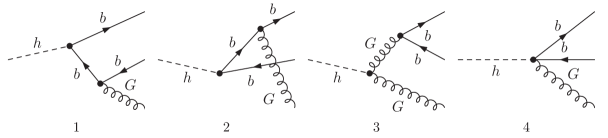
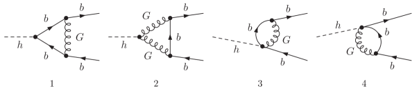
To compute real and virtual amplitudes (squared), the SM and the relevant dimension-6 Lagrangian have been implemented in FeynRules Alloul et al. (2014). The contributing Feynman diagrams are subsequently generated and computed with FeynArts Hahn (2001) and FormCalc Hahn and Perez-Victoria (1999). We show the Feynman diagrams contributing to the real emission amplitude and to the one-loop virtual correction in Fig. 1. We regularise IR divergences which are present individually in both two- and three-body contributions to the decay rate by performing loop integrals and phase-space integrals in dimensions. It is an important check on our calculation that these IR divergences cancel at the level of the decay rate, while UV divergences are removed by the counterterms. A further check is that we reproduce the known SM results as a part of the full SMEFT calculation.
We write the result for the NLO decay rate in the SMEFT in the form
| (21) |
where the first superscript differentiates between the SM and dimension-6 contributions, and the second between powers of . We provide results for the decay rate to as an expansion in , keeping only the leading terms of . The dimension-6 contributions to observables thus appear through the interference of diagrams containing one dimension-6 operator with purely SM diagrams222Additional effects which may appear at , through interference of dimension-6 contributions or the introduction of dimension-8 operators should be investigated if evidence for non-vanishing Wilson coefficients is observed at . .
In writing the results we shall make use of the shorthand notation
| (22) |
Although the computation is performed with complex Wilson coefficients, the result for the decay rate depends only on the real parts of and . To avoid cluttering the notation we do not write out, for instance, , but this is to be understood in all the equations which follow.
The tree-level results for the decay rate are
| (23) |
The QCD corrections for Higgs boson decays to massive quarks within the SM have been known for a long time Braaten and Leveille (1980); Sakai (1980); Inami and Kubota (1981); Drees and Hikasa (1990a, b). The result is
| (24) |
where the kinematic function is given by
| (25) |
The result for the correction to the decay rate in the SMEFT is a function of the Wilson coefficients . The first two appear at tree-level as in Eq. (III), and the latter two contribute for the first time at . The result is
| (26) |
where the contributions to can be deduced from Eq. (II.2).
The expressions above are a main result of this work. We have written the results such that the explicit powers of correspond to those generated by the Yukawa coupling appearing in -vertex, while implicit powers (through, e.g., ) are generated through phase-space factors or through propagators. This will prove convenient when discussing results in the scheme for the -quark mass in the next section. We note that the QCD corrections involving do not factorise explicitly in the above expression, that is, they are not proportional to the SM ones. This is a consequence of renormalising the -quark mass and the Wilson coefficients in different schemes, as we shall see below.
III.1 Results in the scheme and the massless limit
The results presented in the previous section are valid in the on-shell scheme for the masses, and the scheme for the Wilson coefficients. In the presence of a large separation between the scales and , the fixed-order predictions become inappropriate for phenomenology due the appearance of large logarithms of which deteriorate the convergence of the perturbative series in .
To overcome this, the decay rate predictions can be converted into the scheme for the -quark mass (we refer to such predictions as being in the scheme for the decay rate). In this scheme, the dominant large logarithmic corrections are resummed into RG evolution factors relating the value of the running -quark mass at different energy scales. Mass renormalisation in the scheme is achieved by dropping the finite contributions to the -quark mass counterterm in Eq. (II.2). This implies that the relation between the -quark pole mass and mass is
| (27) |
where the SM and dimension-6 contributions to are
| (28) |
We can then define tree-level results in the scheme as333Note that we have not used the mass in the terms, which are related to phase-space factors for on-shell quark production rather than the Yukawa coupling of the Higgs. If the appearing in were also converted, one would need to add extra terms to Eq. (III.1). However, we have checked that the numerical results obtained in that way are nearly identical to those given below, so we have opted for the more streamlined (and physically motivated) version where the phase-space factor is kept in the on-shell scheme.
| (29) |
The corresponding results for the decay rate in the scheme are therefore
| (30) |
where it is understood that in the first term on the right-hand side of each of the above equations. To obtain the leading-logarithmic (LL) solution for the running mass, both SM and dimension-6 corrections to the -quark mass must be taken into account. By inspecting Eq. (27), the following differential equation should be solved
| (31) |
This can be achieved analytically by first finding the LL solution for the running of , and in addition the running -quark mass in the SM — which we label as . In doing so we adopt the following convention for the QCD -function
| (32) |
where the ellipses refer to higher-order terms in and , and , with the number of active flavours. A solution for can easily be obtained when taking into account only the numerically important self-mixing contribution Alonso et al. (2014). This is achieved by solving the equation
| (33) |
We find
| (34) |
Note that our result for differs with respect to that presented in Alonso et al. (2014), since our operator definition in Table 1 implies , where is the definition used in Alonso et al. (2014). Writing
| (35) |
a solution for to can then be obtained as
| (36) |
The motivation for using the scheme for the -quark mass is to resum large logarithms introduced by the scale ratio . Under such circumstances, it also makes sense to consider the massless limit of the decay rate, obtained as , which as we will show below is an excellent approximation numerically. Keeping the first non-vanishing terms in the SM and for each Wilson coefficient in the SMEFT, we find
| (37) |
where we have used
| (38) |
Furthermore, in the massless limit the dimension-6 corrections from to the running mass in Eq. (III.1) vanish. It is worth mentioning that even though the phase-space factor multiplying vanishes as (because of the factor of in Eq. (III)), it is multiplied by a large logarithm in the ratio of , which is not removed by the conversion to the scheme. Finally, in the scheme the coefficients and , which first appear at tree level, receive NLO QCD corrections proportional to the SM ones, while the coefficients and do not.
To test the validity of the massless approximation, we compare numerically the predictions for the total decay rate in the massless limit with the full result. Specifically, we compare
| (39) |
The following set of inputs are used: , GeV, GeV, GeV and GeV. The replacement is made with GeV-2 for numerical evaluation, though the results are presented with an explicit factor of GeV in order compare their size relative to the electroweak scale. We also introduce the dimensionless Wilson coefficients , except for where we also extract the factor of and write . At the scale , and using Eqs. (32), (34) and (III.1) to run the various parameters, we obtain
| (40) |
where we have introduced to highlight the impact of the QCD corrections on the tree-level result. The ellipses denote terms of which are generated by the running -quark mass (see Eq. III.1) and are higher-order in the power counting. The massless limit is therefore found to be an extremely good approximation.
We end this section by commenting on the possible impact of our NLO calculation on global fits to Higgs data. As a concrete example, consider the scenario where a future experiment observes a 5% deviation in the partial width compared to its SM value. Under the assumption that the Wilson coefficients appearing in Eq. (III.1) are , the contributions involving , , can be ignored and only the Wilson coefficient is relevant. The NLO corrections increase the sensitivity to this coefficient by about 20% compared to the LO calculation, and such a measurement on the partial width could be used to probe scales TeV. However, as discussed in Elias-Miro et al. (2013b), in a broad range of UV complete models it is expected that the Wilson coefficient scales as . In that case, even though the prefactor multiplying is about 45 times smaller than that multiplying , the sensitivity to , , and all the other Wilson coefficients is roughly of the same order since , and scales TeV would be probed. A purely LO calculation would miss the contributions from and entirely.
IV Discussion and conclusions
As discussed in the introduction, the Higgs boson couplings are inferred by performing a (global) fit to data of the observable final states. Many groups have now performed dedicated analyses and/or global fits to the LHC Higgs coupling data in an EFT framework Elias-Miro et al. (2013a); Azatov et al. (2012); Espinosa et al. (2012); Plehn and Rauch (2012); Carmi et al. (2012); Peskin (2012); Corbett et al. (2013); Masso and Sanz (2013); Grojean et al. (2013); Falkowski et al. (2013); Dumont et al. (2013); Djouadi and Moreau (2013); Elias-Miro et al. (2013b); Lopez-Val et al. (2013); Pomarol and Riva (2014); Elias-Miro et al. (2014); Englert et al. (2014); Ellis et al. (2014); Belusca-Maito (2014); Ellis et al. (2015); Hartmann and Trott (2015a); Corbett et al. (2015); Hartmann and Trott (2015b); Buchalla et al. (2016); Englert et al. (2015); Aad et al. (2016); Butter et al. (2016); Cirigliano et al. (2016). It should be noted that including constraints from precision electroweak and low-energy observables is also important in a global fit to Higgs data at NLO, since operators which contribute to electroweak precision observables at tree-level can enter the expressions for NLO Higgs decay rates Chen et al. (2014).
An important tool used in several of these global fits is the package eHDECAY Contino et al. (2013, 2014) which allows the computation of Higgs boson decay widths and branching ratios within the SMEFT (implemented in the SILH basis Giudice et al. (2007)). This program is an extension of HDECAY Djouadi et al. (1998); Butterworth et al. (2010), which computes these observables within the SM444Numerical values for a range of inputs have been provided by the LHC Higgs Cross Section Working Group Andersen et al. (2013).. In this case, the expression for the EFT decay rate is obtained by applying a scaling of the tree-level prediction. The scaling factor is the same as that used in the SM, and includes the massless QCD corrections up to Gorishnii et al. (1984, 1991); Kataev and Kim (1994); Surguladze (1994); Larin et al. (1995); Chetyrkin and Kwiatkowski (1996); Chetyrkin (1997); Chetyrkin and Steinhauser (1997); Baikov et al. (2006). This is of course a reasonable procedure, since the QCD corrections to the -vertex involving and factorise, and the most accurate predictions should be applied wherever possible. In addition to the scaled tree-level results, we suggest to include the contributions involving and which are currently not included. The relevant results are provided in Eq. (III.1). It should be noted that the dominant contribution from both of these operators arise from genuine NLO effects, which cannot be predicted by an RG analysis.
Finally, electroweak corrections are known for the decay rate in the SM Fleischer and Jegerlehner (1981); Bardin et al. (1991); Dabelstein and Hollik (1992); Kniehl (1992); Mihaila et al. (2015). However, unlike the QCD corrections involving and , these contributions do not factorise in a straightforward way, and a scaling by known SM corrections is not appropriate. A dedicated calculation of the full NLO electroweak corrections in the SMEFT is in progress. In the meantime, we suggest to include the results involving the one-loop four-fermion and dominant Yukawa corrections which were computed in Gauld et al. (2016). In this case, the running of the -quark mass receives large logarithmic corrections involving the scalar four-fermion operators , and these contributions should be resummed following a similar procedure as was taken for in this work.
V Acknowledgements
The research of D. J. S. is supported by an STFC Postgraduate Studentship.
References
- Aad et al. (2012) G. Aad et al. (ATLAS Collaboration), Phys.Lett. B716, 1 (2012), eprint 1207.7214.
- Chatrchyan et al. (2012) S. Chatrchyan et al. (CMS Collaboration), Phys.Lett. B716, 30 (2012), eprint 1207.7235.
- Bolognesi et al. (2012) S. Bolognesi, Y. Gao, A. V. Gritsan, K. Melnikov, M. Schulze, N. V. Tran, and A. Whitbeck, Phys. Rev. D86, 095031 (2012), eprint 1208.4018.
- Aad et al. (2013) G. Aad et al. (ATLAS), Phys. Lett. B726, 120 (2013), eprint 1307.1432.
- Aad et al. (2015a) G. Aad et al. (ATLAS) (2015a), eprint 1507.04548.
- Khachatryan et al. (2015) V. Khachatryan et al. (CMS), Eur. Phys. J. C75, 212 (2015), eprint 1412.8662.
- ATL (2015) Tech. Rep. ATLAS-CONF-2015-044, CERN, Geneva (2015), URL http://cds.cern.ch/record/2052552.
- Dawson et al. (2013) S. Dawson et al. (2013), eprint 1310.8361, URL http://inspirehep.net/record/1262795/files/arXiv:1310.8361.pdf.
- Andersen et al. (2013) J. R. Andersen et al. (LHC Higgs Cross Section Working Group) (2013), eprint 1307.1347.
- Chatrchyan et al. (2014) S. Chatrchyan et al. (CMS), Phys. Rev. D89, 012003 (2014), eprint 1310.3687.
- Aad et al. (2015b) G. Aad et al. (ATLAS), JHEP 01, 069 (2015b), eprint 1409.6212.
- Dixon and Li (2013) L. J. Dixon and Y. Li, Phys. Rev. Lett. 111, 111802 (2013), eprint 1305.3854.
- Caola and Melnikov (2013) F. Caola and K. Melnikov, Phys. Rev. D88, 054024 (2013), eprint 1307.4935.
- Campbell et al. (2014a) J. M. Campbell, R. K. Ellis, and C. Williams, JHEP 04, 060 (2014a), eprint 1311.3589.
- Campbell et al. (2014b) J. M. Campbell, R. K. Ellis, and C. Williams, Phys. Rev. D89, 053011 (2014b), eprint 1312.1628.
- Campbell et al. (2014c) J. M. Campbell, R. K. Ellis, E. Furlan, and R. Rontsch, Phys. Rev. D90, 093008 (2014c), eprint 1409.1897.
- Englert et al. (2016) C. Englert, M. McCullough, and M. Spannowsky, Nucl. Phys. B902, 440 (2016), eprint 1504.02458.
- Khachatryan et al. (2014) V. Khachatryan et al. (CMS), Phys. Lett. B736, 64 (2014), eprint 1405.3455.
- Aad et al. (2015c) G. Aad et al. (ATLAS), Eur. Phys. J. C75, 335 (2015c), eprint 1503.01060.
- Aicheler et al. (2012) M. Aicheler, M. Aicheler, P. Burrows, M. Draper, T. Garvey, P. Lebrun, K. Peach, N. Phinney, H. Schmickler, D. Schulte, et al. (2012).
- Behnke et al. (2013) T. Behnke, J. E. Brau, B. Foster, J. Fuster, M. Harrison, J. M. Paterson, M. Peskin, M. Stanitzki, N. Walker, and H. Yamamoto (2013), eprint 1306.6327.
- Alexahin et al. (2013) Y. Alexahin et al. (2013), eprint 1308.2143, URL https://inspirehep.net/record/1247266/files/arXiv:1308.2143.pdf.
- Delahaye et al. (2013) J.-P. Delahaye et al. (2013), eprint 1308.0494, URL https://inspirehep.net/record/1246163/files/arXiv:1308.0494.pdf.
- Asner et al. (2003) D. M. Asner, J. B. Gronberg, and J. F. Gunion, Phys. Rev. D67, 035009 (2003), eprint hep-ph/0110320.
- Bogacz et al. (2012) S. A. Bogacz, J. Ellis, L. Lusito, D. Schulte, T. Takahashi, M. Velasco, M. Zanetti, and F. Zimmermann (2012), eprint 1208.2827.
- Baer et al. (2013) H. Baer, T. Barklow, K. Fujii, Y. Gao, A. Hoang, S. Kanemura, J. List, H. E. Logan, A. Nomerotski, M. Perelstein, et al. (2013), eprint 1306.6352.
- Elias-Miro et al. (2013a) J. Elias-Miro, J. R. Espinosa, E. Masso, and A. Pomarol, JHEP 08, 033 (2013a), eprint 1302.5661.
- Elias-Miro et al. (2013b) J. Elias-Miro, J. R. Espinosa, E. Masso, and A. Pomarol, JHEP 11, 066 (2013b), eprint 1308.1879.
- Elias-Miro et al. (2014) J. Elias-Miro, C. Grojean, R. S. Gupta, and D. Marzocca, JHEP 05, 019 (2014), eprint 1312.2928.
- Jenkins et al. (2013) E. E. Jenkins, A. V. Manohar, and M. Trott, JHEP 10, 087 (2013), eprint 1308.2627.
- Jenkins et al. (2014) E. E. Jenkins, A. V. Manohar, and M. Trott, JHEP 01, 035 (2014), eprint 1310.4838.
- Alonso et al. (2014) R. Alonso, E. E. Jenkins, A. V. Manohar, and M. Trott, JHEP 04, 159 (2014), eprint 1312.2014.
- Passarino (2013) G. Passarino, Nucl. Phys. B868, 416 (2013), eprint 1209.5538.
- Chen et al. (2014) C.-Y. Chen, S. Dawson, and C. Zhang, Phys. Rev. D89, 015016 (2014), eprint 1311.3107.
- Grojean et al. (2013) C. Grojean, E. E. Jenkins, A. V. Manohar, and M. Trott, JHEP 04, 016 (2013), eprint 1301.2588.
- Englert and Spannowsky (2015) C. Englert and M. Spannowsky, Phys. Lett. B740, 8 (2015), eprint 1408.5147.
- Zhang (2014a) C. Zhang, J. Phys. Conf. Ser. 556, 012030 (2014a), eprint 1410.2825.
- Pruna and Signer (2014) G. M. Pruna and A. Signer, JHEP 10, 14 (2014), eprint 1408.3565.
- Henning et al. (2014) B. Henning, X. Lu, and H. Murayama (2014), eprint 1412.1837.
- Ghezzi et al. (2015) M. Ghezzi, R. Gomez-Ambrosio, G. Passarino, and S. Uccirati, JHEP 07, 175 (2015), eprint 1505.03706.
- David and Passarino (2015) A. David and G. Passarino (2015), eprint 1510.00414.
- Grober et al. (2015) R. Grober, M. Muhlleitner, M. Spira, and J. Streicher, JHEP 09, 092 (2015), eprint 1504.06577.
- Hartmann and Trott (2015a) C. Hartmann and M. Trott, JHEP 07, 151 (2015a), eprint 1505.02646.
- Hartmann and Trott (2015b) C. Hartmann and M. Trott, Phys. Rev. Lett. 115, 191801 (2015b), eprint 1507.03568.
- Gauld et al. (2016) R. Gauld, B. D. Pecjak, and D. J. Scott, JHEP 05, 080 (2016), eprint 1512.02508.
- Zhang (2016) C. Zhang, Phys. Rev. Lett. 116, 162002 (2016), eprint 1601.06163.
- Maltoni et al. (2016) F. Maltoni, E. Vryonidou, and C. Zhang (2016), eprint 1607.05330.
- Zhang and Maltoni (2013) C. Zhang and F. Maltoni, Phys. Rev. D88, 054005 (2013), eprint 1305.7386.
- Zhang (2014b) C. Zhang, Phys. Rev. D90, 014008 (2014b), eprint 1404.1264.
- Degrande et al. (2015) C. Degrande, F. Maltoni, J. Wang, and C. Zhang, Phys. Rev. D91, 034024 (2015), eprint 1412.5594.
- Buarque Franzosi and Zhang (2015) D. Buarque Franzosi and C. Zhang, Phys. Rev. D91, 114010 (2015), eprint 1503.08841.
- Bessidskaia Bylund et al. (2016) O. Bessidskaia Bylund, F. Maltoni, I. Tsinikos, E. Vryonidou, and C. Zhang, JHEP 05, 052 (2016), eprint 1601.08193.
- Gorbahn and Haisch (2016) M. Gorbahn and U. Haisch (2016), eprint 1607.03773.
- Grzadkowski et al. (2010) B. Grzadkowski, M. Iskrzynski, M. Misiak, and J. Rosiek, JHEP 10, 085 (2010), eprint 1008.4884.
- Wells and Zhang (2015) J. D. Wells and Z. Zhang (2015), eprint 1512.03056.
- Chivukula and Georgi (1987) R. S. Chivukula and H. Georgi, Phys. Lett. B188, 99 (1987).
- D’Ambrosio et al. (2002) G. D’Ambrosio, G. F. Giudice, G. Isidori, and A. Strumia, Nucl. Phys. B645, 155 (2002), eprint hep-ph/0207036.
- Denner (1993) A. Denner, Fortsch. Phys. 41, 307 (1993), eprint 0709.1075.
- Kniehl and Pilaftsis (1996) B. A. Kniehl and A. Pilaftsis, Nucl. Phys. B474, 286 (1996), eprint hep-ph/9601390.
- Alloul et al. (2014) A. Alloul, N. D. Christensen, C. Degrande, C. Duhr, and B. Fuks, Comput. Phys. Commun. 185, 2250 (2014), eprint 1310.1921.
- Hahn (2001) T. Hahn, Comput. Phys. Commun. 140, 418 (2001), eprint hep-ph/0012260.
- Hahn and Perez-Victoria (1999) T. Hahn and M. Perez-Victoria, Comput. Phys. Commun. 118, 153 (1999), eprint hep-ph/9807565.
- Braaten and Leveille (1980) E. Braaten and J. P. Leveille, Phys. Rev. D22, 715 (1980).
- Sakai (1980) N. Sakai, Phys. Rev. D22, 2220 (1980).
- Inami and Kubota (1981) T. Inami and T. Kubota, Nucl. Phys. B179, 171 (1981).
- Drees and Hikasa (1990a) M. Drees and K.-i. Hikasa, Phys. Rev. D41, 1547 (1990a).
- Drees and Hikasa (1990b) M. Drees and K.-i. Hikasa, Phys. Lett. B240, 455 (1990b), [Erratum: Phys. Lett.B262,497(1991)].
- Azatov et al. (2012) A. Azatov, R. Contino, and J. Galloway, JHEP 04, 127 (2012), [Erratum: JHEP04,140(2013)], eprint 1202.3415.
- Espinosa et al. (2012) J. R. Espinosa, C. Grojean, M. Muhlleitner, and M. Trott, JHEP 12, 045 (2012), eprint 1207.1717.
- Plehn and Rauch (2012) T. Plehn and M. Rauch, Europhys. Lett. 100, 11002 (2012), eprint 1207.6108.
- Carmi et al. (2012) D. Carmi, A. Falkowski, E. Kuflik, T. Volansky, and J. Zupan, JHEP 10, 196 (2012), eprint 1207.1718.
- Peskin (2012) M. E. Peskin (2012), eprint 1207.2516.
- Corbett et al. (2013) T. Corbett, O. J. P. Eboli, J. Gonzalez-Fraile, and M. C. Gonzalez-Garcia, Phys. Rev. D87, 015022 (2013), eprint 1211.4580.
- Masso and Sanz (2013) E. Masso and V. Sanz, Phys. Rev. D87, 033001 (2013), eprint 1211.1320.
- Falkowski et al. (2013) A. Falkowski, F. Riva, and A. Urbano, JHEP 11, 111 (2013), eprint 1303.1812.
- Dumont et al. (2013) B. Dumont, S. Fichet, and G. von Gersdorff, JHEP 07, 065 (2013), eprint 1304.3369.
- Djouadi and Moreau (2013) A. Djouadi and G. Moreau, Eur. Phys. J. C73, 2512 (2013), eprint 1303.6591.
- Lopez-Val et al. (2013) D. Lopez-Val, T. Plehn, and M. Rauch, JHEP 10, 134 (2013), eprint 1308.1979.
- Pomarol and Riva (2014) A. Pomarol and F. Riva, JHEP 01, 151 (2014), eprint 1308.2803.
- Englert et al. (2014) C. Englert, A. Freitas, M. M. Muhlleitner, T. Plehn, M. Rauch, M. Spira, and K. Walz, J. Phys. G41, 113001 (2014), eprint 1403.7191.
- Ellis et al. (2014) J. Ellis, V. Sanz, and T. You, JHEP 07, 036 (2014), eprint 1404.3667.
- Belusca-Maito (2014) H. Belusca-Maito (2014), eprint 1404.5343.
- Ellis et al. (2015) J. Ellis, V. Sanz, and T. You, JHEP 03, 157 (2015), eprint 1410.7703.
- Corbett et al. (2015) T. Corbett, O. J. P. Eboli, D. Goncalves, J. Gonzalez-Fraile, T. Plehn, and M. Rauch, JHEP 08, 156 (2015), eprint 1505.05516.
- Buchalla et al. (2016) G. Buchalla, O. Cata, A. Celis, and C. Krause, Eur. Phys. J. C76, 233 (2016), eprint 1511.00988.
- Englert et al. (2015) C. Englert, R. Kogler, H. Schulz, and M. Spannowsky (2015), eprint 1511.05170.
- Aad et al. (2016) G. Aad et al. (ATLAS), Phys. Lett. B753, 69 (2016), eprint 1508.02507.
- Butter et al. (2016) A. Butter, O. J. P. Eboli, J. Gonzalez-Fraile, M. C. Gonzalez-Garcia, T. Plehn, and M. Rauch (2016), eprint 1604.03105.
- Cirigliano et al. (2016) V. Cirigliano, W. Dekens, J. de Vries, and E. Mereghetti (2016), eprint 1605.04311.
- Contino et al. (2013) R. Contino, M. Ghezzi, C. Grojean, M. Muhlleitner, and M. Spira, JHEP 07, 035 (2013), eprint 1303.3876.
- Contino et al. (2014) R. Contino, M. Ghezzi, C. Grojean, M. Muhlleitner, and M. Spira, Comput. Phys. Commun. 185, 3412 (2014), eprint 1403.3381.
- Giudice et al. (2007) G. F. Giudice, C. Grojean, A. Pomarol, and R. Rattazzi, JHEP 06, 045 (2007), eprint hep-ph/0703164.
- Djouadi et al. (1998) A. Djouadi, J. Kalinowski, and M. Spira, Comput. Phys. Commun. 108, 56 (1998), eprint hep-ph/9704448.
- Butterworth et al. (2010) J. M. Butterworth et al. (2010), eprint 1003.1643, URL https://inspirehep.net/record/848006/files/arXiv:1003.1643.pdf.
- Gorishnii et al. (1984) S. G. Gorishnii, A. L. Kataev, and S. A. Larin, Sov. J. Nucl. Phys. 40, 329 (1984), [Yad. Fiz.40,517(1984)].
- Gorishnii et al. (1991) S. G. Gorishnii, A. L. Kataev, S. A. Larin, and L. R. Surguladze, Phys. Rev. D43, 1633 (1991).
- Kataev and Kim (1994) A. L. Kataev and V. T. Kim, Mod. Phys. Lett. A9, 1309 (1994).
- Surguladze (1994) L. R. Surguladze, Phys. Lett. B341, 60 (1994), eprint hep-ph/9405325.
- Larin et al. (1995) S. A. Larin, T. van Ritbergen, and J. A. M. Vermaseren, Phys. Lett. B362, 134 (1995), eprint hep-ph/9506465.
- Chetyrkin and Kwiatkowski (1996) K. G. Chetyrkin and A. Kwiatkowski, Nucl. Phys. B461, 3 (1996), eprint hep-ph/9505358.
- Chetyrkin (1997) K. G. Chetyrkin, Phys. Lett. B390, 309 (1997), eprint hep-ph/9608318.
- Baikov et al. (2006) P. A. Baikov, K. G. Chetyrkin, and J. H. Kuhn, Phys. Rev. Lett. 96, 012003 (2006), eprint hep-ph/0511063.
- Chetyrkin and Steinhauser (1997) K. G. Chetyrkin and M. Steinhauser, Phys. Lett. B408, 320 (1997), eprint hep-ph/9706462.
- Fleischer and Jegerlehner (1981) J. Fleischer and F. Jegerlehner, Phys. Rev. D23, 2001 (1981).
- Bardin et al. (1991) D. Yu. Bardin, B. M. Vilensky, and P. K. Khristova, Sov. J. Nucl. Phys. 53, 152 (1991), [Yad. Fiz.53,240(1991)].
- Dabelstein and Hollik (1992) A. Dabelstein and W. Hollik, Z. Phys. C53, 507 (1992).
- Kniehl (1992) B. A. Kniehl, Nucl. Phys. B376, 3 (1992).
- Mihaila et al. (2015) L. Mihaila, B. Schmidt, and M. Steinhauser, Phys. Lett. B751, 442 (2015), eprint 1509.02294.