Performance of Massive MIMO Uplink with Zero-Forcing receivers under Delayed Channels

Abstract

In this paper, we analyze the performance of the uplink communication of massive multi-cell multiple-input multiple-output (MIMO) systems under the effects of pilot contamination and delayed channels because of terminal mobility. The base stations (BSs) estimate the channels through the uplink training, and then use zero-forcing processing to decode the transmit signals from the users. The probability density function (PDF) of the signal-to-interference-plus-noise ratio is derived for any finite number of antennas. From this PDF, we derive an achievable ergodic rate with a finite number of BS antennas in closed form. Insights of the impact of the Doppler shift (due to terminal mobility) at the low signal-to-noise ratio regimes are exposed. In addition, the effects on the outage probability are investigated. Furthermore, the power scaling law and the asymptotic performance result by infinitely increasing the numbers of antennas and terminals (while their ratio is fixed) are provided. The numerical results demonstrate the performance loss for various Doppler shifts. Among the interesting observations revealed is that massive MIMO is favorable even in channel aging conditions.

I Introduction

The rapidly increasing demand for wireless connectivity and throughput is one of the motivations for the continuous evolution of cellular networks [2, 3]. Massive multiple-input multiple-output (MIMO) has been considered as a new promising breakthrough technology due to its ability for achieving huge spectral and energy efficiencies [4, 5, 6, 7]. Its origin is found in [4], and it has been given many alternative names such as very large multi-user MIMO, hyper-MIMO, or full-dimension MIMO systems. In the typical envisioned architecture, each base station (BS) with an array of hundreds or even thousands of antennas, exploiting the key idea of multi-user MIMO, coherently serves tens or hundreds of single-antenna terminals simultaneously in the same frequency band, respectively. This difference in the number of BS antennas $N$ and the number of terminals $K$ per cell provides unprecedented spatial degrees of freedom that leads to a high throughput, allowing, in addition, low-complexity linear signal processing techniques and avoiding inter-user interference because of the (near) Unfortunately, a fundamental degradation, known as pilot contamination, degrades the performance of massive MIMO systems. It emerges from the re-use of the pilot sequences in other cells, and results in inter-cell interference, even when the number of antennas becomes very large.

In massive MIMO, zero-forcing (ZF) processing is preferable since it has low complexity and its performance is very close to that of maximum-likelihood multi-user decoder and “dirty paper coding” [8]. Plenty of research is dedicated to single-cell networks with ZF receivers [9], and also to multi-cell systems with perfect channel state information (CSI) [10] and with the arising pilot contamination [11].

Despite that the theory of massive MIMO has been now well established (see [4] and references therein), the impact of channel aging coming from the relative movement of terminals on massive MIMO systems lacks investigation in the literature. Channel aging problem occurs in practical scenarios, e.g. in an urban area, where the mobility of terminals is high. The fundamental challenge in these environments is how to estimate the channel efficiently. To model the impact of terminal mobility, a stationary ergodic Gauss-Markov block fading [12, 13, 15, 16, 17, 18] is often used. With this channel, an autoregressive model is associated with the Jakes’ autocorrelation function which represents the channel time variation.

It is known that the channel estimation overhead is independent of the number of BS antennas, but it is proportional to the number of terminals. The number of terminals that can be served depends on the length of each frame which is designed based on the user mobility. Specifically, the higher the mobility of terminals is, the smaller the frame length is, which in turn degrades the system performance due to pilot contamination (since fewer pilots can be sent). Furthermore, an increase of the user mobility hampers the quality of channel estimation because the time variation of the channel increases, and thus, the constructed decoders and precoders lack precision. Driven by these observations, this paper investigates the robustness of massive MIMO against the practical setting of terminal mobility that results in delayed and degraded CSI at the BS, and thus, imperfect CSI. Such consideration is notably important because it can provide the quantification of the performance loss in various Doppler shifts. A limited effort for studying the time variation of the channel because of the relative movement of terminals has taken place in [13], where the authors provided deterministic equivalents (DEs) for the maximal-ratio-combining (MRC) receivers in the uplink and the maximal-ratio-transmission (MRT) precoders in the downlink. This analysis was extended in [16, 15] by deriving DEs for the minimum mean-square error (MMSE) receivers (for the uplink) and regularized zero-forcing (for the downlink). In this paper, extending [1], we elaborate further on a generalized massive MIMO system uplink. Based on the aforementioned literature, we propose a tractable model that encompasses ZF receivers and describes the impact of terminal mobility in a multicell system with an arbitrary number of BS antennas and terminals, which distinguishes it from previous works. The following are the main contributions of this paper:

• In contrast to [10], which assumes perfect CSI, we consider more practical settings where the channel is imperfectly estimated at the BS. The effects of pilot contamination and channel time variation are taken into account. The extension is not straightforward because apart from the development of the model, the mathematical manipulations are more difficult. Apart of this, the results are contributory and novel.

• We derive the probability density function (PDF) of the signal-to-interference-plus-noise ratio (SINR), the corresponding ergodic rate, and the outage probability for any finite number of antennas in closed forms. For the sake of completeness, the link of these results with previously known results is mentioned. Furthermore, a simpler and more tractable lower bound for the achievable uplink rate is derived.

• We elaborate on the low signal-to-noise ratio (SNR) regime, in order to get additional insights into the impact of Doppler shift. In particular, we study the behaviors of the minimum normalized energy per information bit to reliably convey any positive rate and the wideband slope.

• We evaluate the asymptotic performance for the case where the number of BS antennas $N\to\infty$ and for the case where both the number of BS antennas $N$ and the number of the terminals $K$ go to infinity. This analysis aims at providing accurate approximation results that replace the need for lengthy Monte Carlo simulations.

Note that, although all the results incur significant mathematical challenges, they can be easily evaluated. Moreover, the motivation behind the use of DEs is to provide deterministic tight approximations, in order to avoid lengthy Monte-Carlo simulations.

The rest of this paper is structured as follows: Section II presents the system model for the uplink of cellular systems with ZF receivers. In Section III, we provide the main results regarding the achievable uplink rate, its simple tight lower bound, and the outage probability. Furthermore, we shed light on the low-SNR regime of the system, and we investigate both the large number of antennas and large system (large number of antennas and users) limits. The numerical results are discussed in Section IV, while Section V summarizes the paper.

Notation: For matrices and vectors, we use boldface uppercase and lowercase letters, respectively. The notations $(\cdot)^{\scriptscriptstyle\mathsf{H}}$ and $(\cdot)^{\dagger}$ stand for the conjugate transpose and the pseudo-inverse of a matrix as well as the Euclidean norm of a vector is denoted by $\|\cdot\|$. The notation $x\overset{\tt d}{\sim}y$ is used to denote that $x$ and $y$ have the same distribution. Finally, we use ${\color[rgb]{0.00,0.00,1.00}\mathbf{z}}\sim\mathcal{CN}\left({\mathbf{0}},{{\boldsymbol{\Sigma}}}\right)$ to denote a circularly symmetric complex Gaussian vector $\mathbf{z}$ with zero mean and covariance matrix ${\boldsymbol{\Sigma}}$.

$$\gamma_{k}\!=\!\frac{\alpha^{2}p_{r}}{\alpha^{2}p_{r}\sum_{i\neq l}^{L}\!\left\|\!\left[\hat{{\boldsymbol{G}}}_{ll}^{\dagger}[n\!-\!1]\right]_{k}\!\hat{{\boldsymbol{G}}}_{li}[n\!-\!1]\right\|^{2}\!+\!p_{r}\sum_{i=l}^{L}\!\left\|\!\left[\hat{{\boldsymbol{G}}}_{ll}^{\dagger}[n\!-\!1]\right]_{k}\!\tilde{{\boldsymbol{E}}}_{li}[n]\!\right\|^{2}\!+\!\left\|\!\left[\hat{{\boldsymbol{G}}}_{ll}^{\dagger}[n\!-\!1]\right]_{k}\!\right\|^{2}}.$$ (13)

II System Model

We focus on a cellular network which has $L$ cells. Each cell includes one $N$-antenna BS and $K$ single-antenna terminals. We elaborate on the uplink transmission. The model is based on the assumptions that: i) $N\geq K$, and ii) all terminals in $L$ cells share the same time-frequency resource. Furthermore, we hypothesize that the channels change from symbol to symbol under the channel aging impact [13] (we will discuss the channel aging model later).

Denote by ${\boldsymbol{g}}_{lik}[n]\in\mathbb{C}^{N\times 1}$ the channel vector between the $l$th BS and the $k$th terminal in the $i$th cell at the $n$th symbol. The channel ${\boldsymbol{g}}_{lik}[n]\in\mathbb{C}^{N\times 1}$ is modeled by large-scale fading (path loss and shadowing) and small-scale fading as follows:

$${\boldsymbol{g}}_{lik}[n]=\sqrt{\beta_{lik}}{\boldsymbol{h}}_{lik}[n],$$ (1)

where $\beta_{lik}$ represents large-scale fading, and ${\boldsymbol{h}}_{lik}\in\mathbb{C}^{N\times 1}$ is the small-scale fading vector between the $l$th BS and the $k$th terminal in the $i$th cell with ${\boldsymbol{h}}_{lik}\sim\mathcal{CN}\left({{\boldsymbol{0}}},{{\bm{\mathrm{I}}}_{N}}\right)$.

Let $\sqrt{p_{r}}{\boldsymbol{x}}_{i}[n]\in\mathbb{C}^{K\times 1}$ be the vector of transmit signals from the $K$ terminals in the $i$th cell at time instance $n$ ($p_{r}$ is the average transmit power of each terminal. Elements of ${\boldsymbol{x}}_{i}[n]$ are assumed to be i.i.d. zero-mean and unit variance random variables (RVs). Then, the $N\times 1$ received signal vector at the $l$th BS is

$${\boldsymbol{y}}_{l}[n]=\sqrt{p_{r}}\sum_{i=1}^{L}{\boldsymbol{G}}_{li}[n]{\boldsymbol{x}}_{i}[n]+{\boldsymbol{z}}_{l}[n],~{}~{}~{}l=1,2,...,L,$$ (2)

where ${\boldsymbol{G}}_{li}[n]\triangleq\left[{\boldsymbol{g}}_{li1}[n],\ldots,{\boldsymbol{g}}_{liK}[n]\right]\in\mathbb{C}^{N\times K}$ denotes the channel matrix between the $l$th BS and the $K$ terminals in the $i$th cell, and ${\boldsymbol{z}}_{l}[n]\sim\mathcal{CN}\left({{\boldsymbol{0}}},{{\bm{\mathrm{I}}}_{N}}\right)$ is the noise vector at the $l$th BS.

II-A Uplink Training

To coherently detect the transmit signals from the $K$ terminals in the $l$th cell, the BS needs CSI knowledge. Typically, the $l$th BS can estimate the channels from the uplink pilots. During the training phase, we assume that the channel does not change, neglecting an error due to the channel aging effect [13]. In general, this assumption is not practical, but it yields a simple model which enables us to analyze the system performance and to obtain initial insights on the impact of channel aging. It is shown in [14] that, in most cases, the additional error term in the channel estimate which comes from the channel aging effect during the training phase can be neglected. In some cases, the investigation of the effect of this error is interesting. However, it yields a complicated model which is intractable for analysis. We leave this investigation for future work.

In the training phase, $K$ terminals in each cell are assigned $K$ orthogonal pilot sequences, each has a length of $\tau$ symbols (it requires $\tau\geq K$). Owing to the limitation of the frame length, the pilot sequences of all terminals in all cells cannot be pairwisely orthogonal. We assume that the orthogonal pilot sequences are reused from cell to cell (i.e., all $L$ cells use the same set of $K$ orthogonal pilot sequences). As a result, pilot contamination occurs [4]. Let ${\boldsymbol{\Psi}}\in\mathbb{C}^{K\times\tau}$ be the pilot matrix transmitted from the $K$ terminals in each cell, where the $k$th row of ${\boldsymbol{\Psi}}$ is the pilot sequence assigned for the $k$th terminal. The matrix ${\boldsymbol{\Psi}}$ satisfies ${\boldsymbol{\Psi}}{\boldsymbol{\Psi}}^{\scriptscriptstyle\mathsf{H}}={\bm{\mathrm{I}}}_{K}$. Then, the $N\times\tau$ received pilot signal at the $l$th BS is given by

$${\boldsymbol{Y}}^{\mathrm{tr}}_{l}[n]=\sqrt{p_{\mathrm{tr}}}\sum_{i=1}^{L}{\boldsymbol{G}}_{li}[n]{\boldsymbol{\Psi}}+{\boldsymbol{Z}}^{\mathrm{tr}}_{l}[n],~{}~{}~{}l=1,2,...,L,$$ (3)

where the superscript and subscript “$\mathrm{tr}$” imply the uplink training, ${p_{\mathrm{tr}}}\triangleq\tau{p_{r}}$, and ${\boldsymbol{Z}}_{l}^{\mathrm{tr}}[n]\in\mathbb{C}^{N\times\tau}$ is the additive noise. We consider that the elements of ${\boldsymbol{Z}}^{\mathrm{tr}}_{l}[n]$ are i.i.d. $\mathcal{CN}\left({0},{1}\right)$ RVs. With MMSE channel estimation scheme, the estimate of ${{\boldsymbol{g}}}_{lik}[n]$ is [6]

$$\hat{{\boldsymbol{g}}}_{lik}[n]= \beta_{lik}{\boldsymbol{Q}}_{lk}\left(\sum_{j=1}^{L}{\boldsymbol{g}}_{ljk}[n]+\frac{1}{\sqrt{p_{\mathrm{tr}}}}\tilde{{\boldsymbol{z}}}^{\mathrm{tr}}_{lk}[n]\right)\!\!,$$ (4)

where ${\boldsymbol{Q}}_{lk}\!\triangleq\!\left(\frac{1}{p_{\mathrm{tr}}}\!+\!\sum_{i=1}^{L}\beta_{lik}\right)^{\!-1}\!{\bm{\mathrm{I}}}_{N}$, and $\tilde{{\boldsymbol{z}}}^{\mathrm{tr}}_{lk}[n]\!\sim\!\mathcal{CN}\!\left({\boldsymbol{0}},{\bm{\mathrm{I}}}_{N}\right)$ represents the noise which is independent of ${\boldsymbol{g}}_{ljk}[n]$. Let $\hat{{\boldsymbol{G}}}_{li}[n]\triangleq\left[\hat{{\boldsymbol{g}}}_{li1}[n],\ldots,\hat{{\boldsymbol{g}}}_{liK}[n]\right]\in\mathbb{C}^{N\times K}$. Then, $\hat{{\boldsymbol{G}}}_{li}[n]$ can be given by

$$\hat{{\boldsymbol{G}}}_{li}[n]=\hat{{\boldsymbol{G}}}_{ll}[n]{\boldsymbol{{D}}}_{i},$$ (5)

where ${\boldsymbol{{D}}}_{i}=\mathrm{diag}\big{\{}\frac{{\beta}_{li1}}{{\beta}_{ll1}},\frac{{\beta}_{li2}}{{\beta}_{ll2}},\ldots,\frac{{\beta}_{liK}}{{\beta}_{llK}}\big{\}}$.

From the property of MMSE channel estimation, the channel estimation error and the channel estimate are independent. Thus, ${\boldsymbol{g}}_{lik}[n]$ can be rewritten as:

$${\boldsymbol{g}}_{lik}[n]=\hat{{\boldsymbol{g}}}_{lik}[n]+\tilde{{\boldsymbol{g}}}_{lik}[n],$$ (6)

where $\tilde{{\boldsymbol{g}}}_{lik}[n]$ and $\hat{{\boldsymbol{g}}}_{lik}[n]$ are the independent channel estimation error and channel estimate, respectively. Furthermore, we have $\tilde{{\boldsymbol{g}}}_{lik}[n]\sim\mathcal{CN}\left({{\boldsymbol{0}}},{\left(\beta_{lik}-\hat{\beta}_{lik}\right){\boldsymbol{\mathrm{I}}}_{N}}\right)$ and $\hat{{\boldsymbol{g}}}_{lik}[n]\sim\mathcal{CN}\left({{\boldsymbol{0}}},{\hat{\beta}_{lik}}\right)$, where $\hat{\beta}_{lik}\triangleq\frac{\beta^{2}_{lik}}{\sum_{j=1}^{L}\beta_{ljk}+1/p_{\mathrm{tr}}}$. Here we assume that $\beta_{lik}$, $\hat{\beta}_{lik}$, and ${\boldsymbol{Q}}_{lk}$ are independent of $n$ $\forall l$, $i$, and $k$. This assumption is reasonable since these values depend on large-scale fading which changes very slowly with time.

II-B Delayed Channel Model

Besides pilot contamination, in any common propagation scenario, a relative movement takes place between the antennas and the scatterers that degrades more channel’s performance. Under these circumstances, the channel is time-varying and needs to be modeled by the famous Gauss-Markov block fading model, which is basically an autoregressive model of certain order that incorporate two-dimensional isotropic scattering (Jakes model). More specifically, our analysis achieves to express the current channel state in terms of its past samples. For the sake of tractable analytical and computational simplicity, we focus on the following simplified autoregressive model of order $1$ [12, 13, 15, 16, 17, 18]

$${\boldsymbol{g}}_{lik}[n]=\alpha{{\boldsymbol{g}}}_{lik}[n-1]+{\boldsymbol{e}}_{lik}[n],$$ (7)

where ${\boldsymbol{e}}_{lik}[n]\sim\mathcal{CN}\left({{\boldsymbol{0}}},{\left(1-\alpha^{2}\right)\beta_{lik}{\boldsymbol{\mathrm{I}}}_{N}}\right)$ is the stationary Gaussian channel error vector because of the time variation of the channel, independent of ${{\boldsymbol{g}}}_{lik}[n-1]$. In (7), $\alpha$ is the temporal correlation parameter, given by

$$\alpha\!=\!\mathrm{J}_{0}\left(2\pi f_{D}T_{s}\right),$$ (8)

where $\mathrm{J}_{0}(\cdot)$ is the zeroth-order Bessel function of the first kind, $f_{D}$ is the maximum Doppler shift, and $T_{s}$ is the channel sampling period. The maximum Doppler shift $f_{D}$ is equal to $\frac{vf_{c}}{c}$, where $v$ is the relative velocity of the terminal, $c$ is the speed of light, and $f_{c}$ is the carrier frequency. It is assumed that $\alpha$ is accurately obtained at the BS via a rate-limited backhaul link.

Plugging (6) into (7), we obtain a model which represents both effects of channel estimation error due to pilot contamination and channel aging:

$${\boldsymbol{g}}_{lik}[n] =\alpha{{\boldsymbol{g}}}_{lik}[n-1]+{\boldsymbol{e}}_{lik}[n]$$

$$=\alpha\hat{{\boldsymbol{g}}}_{lik}[n-1]+\tilde{{\boldsymbol{e}}}_{lik}[n],$$ (9)

where $\tilde{{\boldsymbol{e}}}_{lik}[n]\triangleq\alpha\tilde{{\boldsymbol{g}}}_{lik}[n-1]+{\boldsymbol{e}}_{lik}[n]\sim\mathcal{CN}\left({{\boldsymbol{0}}},{\left(\beta_{lik}-\alpha^{2}\hat{\beta}_{lik}\right){\boldsymbol{\mathrm{I}}}_{N}}\right)$ is independent of $\hat{{\boldsymbol{g}}}_{lik}[n-1]$.

II-C Zero-Forcing Receiver

Substituting (9) into (2), the received signal at the $l$th BS can be rewritten as

$${\boldsymbol{y}}_{l}[n]\!=\!\alpha\sqrt{p_{r}}\sum_{i=1}^{L}\!{\boldsymbol{\hat{G}}}_{li}[n\!-\!1]{\boldsymbol{x}}_{i}[n]+\sqrt{p_{r}}\sum_{i=1}^{L}\!{\boldsymbol{\tilde{E}}}_{li}[n]{\boldsymbol{x}}_{i}[n]\!+\!{\boldsymbol{z}}_{l}[n],$$ (10)

where $\tilde{{\boldsymbol{E}}}_{li}\triangleq\left[\tilde{{\boldsymbol{e}}}_{li1}[n],\ldots,\tilde{{\boldsymbol{e}}}_{liK}[n]\right]\in\mathbb{C}^{N\times K}$. With ZF processing, the received signal ${\boldsymbol{y}}_{l}[n]$ is first multiplied with $\alpha^{-1}\hat{{\boldsymbol{G}}}_{ll}^{\dagger}[n-1]$ as follows:

$$\!{\boldsymbol{r}}_{l}[n]=\sqrt{p_{r}}{\boldsymbol{x}}_{l}[n]+\sqrt{p_{r}}\sum_{i\neq l}^{L}\hat{{\boldsymbol{G}}}_{ll}^{\dagger}[n-1]{\boldsymbol{\hat{G}}}_{li}[n-1]{\boldsymbol{x}}_{i}[n]$$

$$\!+\!\alpha^{\!-\!1}\!\sqrt{p_{r}}\sum_{i=1}^{L}\!\hat{{\boldsymbol{G}}}_{ll}^{\dagger}[n\!-\!1]{\boldsymbol{\tilde{E}}}_{li}[n]{\boldsymbol{x}}_{i}[n]\!+\!\alpha^{\!-\!1}\hat{{\boldsymbol{G}}}_{ll}^{\dagger}[n\!-\!1]{\boldsymbol{z}}_{l}[n].$$ (11)

Then, the $k$th element of ${\boldsymbol{r}}_{l}[n]$ is used to decode the transmit signal from the $k$th terminal, ${x}_{lk}[n]$. The $k$th element of ${\boldsymbol{r}}_{l}[n]$ is

$$\!\!\!{r}_{lk}[n]=\sqrt{p_{r}}{x}_{lk}[n]\!+\!\sqrt{p_{r}}\!\sum_{i\neq l}^{L}\!\left[\hat{{\boldsymbol{G}}}_{ll}^{\dagger}[n-1]\right]_{k}\!{\boldsymbol{\hat{G}}}_{li}[n\!-\!1]{\boldsymbol{x}}_{i}[n]$$

$$\!\!\!+\!\frac{1}{\alpha}\!\sqrt{p_{r}}\!\!\sum_{i=1}^{L}\!\left[\hat{{\boldsymbol{G}}}_{ll}^{\dagger}[n\!-\!1]\right]_{k}\!\!{\boldsymbol{\tilde{E}}}_{li}[n]{\boldsymbol{x}}_{i}[n]\!+\!\frac{1}{\alpha}\!\!\left[\hat{{\boldsymbol{G}}}_{ll}^{\dagger}[n\!-\!1]\right]_{k}\!{\boldsymbol{z}}_{l}[n],$$ (12)

where $\left[{\boldsymbol{A}}\right]_{k}$ denotes the $k$th row of matrix ${\boldsymbol{A}}$, and ${x}_{lk}[n]$ is the $k$th element of ${\boldsymbol{x}}_{l}[n]$. By treating (II-C) as a single-input single-output (SISO) system, we obtain the SINR of the transmission from the $k$th user in the $l$th cell to its BS given by (13) shown at the top of the previous page. Henceforth, we assume that this SINR is obtained under the assumption that the $l$th BS does not need the instantaneous knowledge of the terms in the denominator of (13), but only of their statistics, which can be easily acquired, especially, if they change over a long-time scale. More specifically, the BS knows the probability distribution of the actual channel given the available estimate, i.e., if we denote the probability $p$, we have $P_{{\boldsymbol{G}}|\hat{{\boldsymbol{G}}}}=p_{\tilde{{\boldsymbol{E}}}}=p_{({\boldsymbol{G}}-\hat{{\boldsymbol{G}}})}$.

$$\mathcal{J}_{m,n}\left(a,b,\alpha\right) \triangleq\sum_{r=0}^{m}\binom{m}{r}\left(-b\right)^{m-r}\left[\sum_{s=0}^{n+r}\frac{\left(n+r\right)^{s}b^{n+r-s}}{\alpha^{s+1}a^{m-s}}\mathrm{Ei}\left(\!-b\right)-\frac{\left(n+r\right)^{n+r}e^{\alpha b/a}}{\alpha^{n+r+1}a^{m-n-r}}\mathrm{Ei}\left(\!-\frac{\alpha b}{a}-b\!\right)\right.$$

$$\hskip 128.0374pt\left.+\frac{e^{-b}}{\alpha}\sum_{s=0}^{n+r-1}\sum_{u=0}^{n+r-s-1}\frac{u!\left(n+r\right)^{s}\binom{n+r-s-1}{u}b^{n+r-s-u-1}}{\alpha^{s}a^{m-s}\left(\alpha/a+1\right)^{s+1}}\right].$$ (18)

III Achievable Uplink Rate

This section provides the achievable rate analysis for finite and infinite number of BS antennas by accomodating the effects of pilot contamination and channel aging.

III-A Finite-$N$ Analysis

Denote by $\mathbf{\mathcal{A}}_{k}\triangleq\mathrm{diag}\left(\tilde{{\boldsymbol{D}}}_{l1},\ldots,\tilde{{\boldsymbol{D}}}_{lL}\right)$, where $\tilde{{\boldsymbol{D}}}_{li}$ a $K\times K$ diagonal matrix whose $k$th diagonal element is $\left[\tilde{{\boldsymbol{D}}}_{li}\right]_{kk}=\left(\beta_{lik}-\alpha^{2}\hat{\beta}_{lik}\right)$. Then the distribution of the SINR for the uplink transmission from the $k$th terminal is given in the following proposition.

Proposition 1

The SINR of transmission from the $k$th terminal in the $l$th cell to its BS, under the delayed channels, is distributed as

$$\gamma_{k}\mathop{\sim}\limits^{\tt d}\frac{\alpha^{2}p_{r}X_{k}[n-1]}{\alpha^{2}p_{r}CX_{k}[n-1]+p_{r}Y_{k}[n]+1},$$ (14)

where $C\triangleq\sum_{i\neq l}^{L}\left(\frac{\beta_{lik}}{\beta_{llk}}\right)^{2}$ is a deterministic constant, $X_{k}$ and $Y_{k}$ are independent RVs whose PDFs are, respectively, given by

$$\!\!p_{{X_{k}}}\left({x}\right) \!=\!\frac{e^{-x/\hat{\beta}_{llk}}}{\left(N-K\right)!\hat{\beta}_{llk}}\left(\frac{x}{\hat{\beta}_{llk}}\right)^{N-K},~{}x\geq 0,$$ (15)

$$\!\!p_{{Y_{k}}}\left({y}\right) \!=\!\!\sum_{p=1}^{\varrho\left(\!\mathbf{\mathcal{A}}_{k}\!\right)}\!\sum_{q=1}^{\tau_{p}\left(\!\mathbf{\mathcal{A}}_{k}\!\right)}\!\!\!\!\mathcal{X}_{p,q}\left(\!\mathbf{\mathcal{A}}_{k}\!\right)\!\frac{\mu_{k,p}^{-q}}{\left(q\!-\!1\right)!}y^{q-1}e^{\frac{-y}{\mu_{k,p}}},~{}y\geq 0.$$ (16)

In (16), $\mathcal{X}_{p,q}\left(\mathbf{\mathcal{A}}_{k}\right)$ is the $\left(p,q\right)$th characteristic coefficients of $\mathbf{\mathcal{A}}_{k}$, defined in [19, Definition 4]; $\varrho\left(\mathbf{\mathcal{A}}_{k}\right)$ is the numbers of distinct diagonal elements of $\mathbf{\mathcal{A}}_{k}$; $\mu_{k,1},...,\mu_{k,\varrho\left(\mathbf{\mathcal{A}}_{k}\right)}$ are the distinct diagonal elements of $\mathbf{\mathcal{A}}_{k}$ in decreasing order; and $\tau_{p}\left(\mathbf{\mathcal{A}}_{k}\right)$ are the multiplicities of $\mu_{k,p}$.

Proof 1

See Appendix -A.

Remark 1

Following the behavior of the Bessel function $\mathrm{J}_{0}(\cdot)$, the SINR presents ripples with zero and peak points with respect to the relative velocity of the user with respect to the BS. In the extreme case of $\alpha=1$ (corresponding to the case where there is no relative movement of the terminal), (14) represents the result for the case of without channel aging impact. In another extreme case where $\alpha\to 0$ (i.e. velocity is very high), SINR becomes zero. Furthermore, if we assume no time variation and the training intervals can be long enough so that all pilot sequences are orthogonal, our result coincides with [10, Eq. (6)].

Corollary 1

When the uplink power grows large, the SINR $\gamma_{k}$ is bounded:

$$\gamma_{k}\big{|}_{p_{r}\rightarrow\infty}\mathop{\sim}\limits^{\tt d}\frac{\alpha^{2}X_{k}[n-1]}{\alpha^{2}CX_{k}[n-1]+Y_{k}[n]}.$$ (17)

Corollary 1 brings an important insight on the system performance, when $p_{r}$ is large. As seen in (17), there is a finite SINR ceiling when $p_{r}\to\infty$, which emerges because of the simultaneous increases of the desired signal power and the interference powers when $p_{r}$ increases.

Having obtained the PDF of the SINR, and by defining the function $\mathcal{J}_{m,n}\left(a,b,\alpha\right)$ as in (18) shown at the top of the next page, where $\mathrm{Ei}\left(\cdot\right)$ denotes the exponential integral function [22, Eq. (8.211.1)], we first obtain the exact $R_{lk}\left(p_{r},\alpha\right)$ and a simpler lower bound $R_{L}\left(p_{r},\alpha\right)$ as follows:

Theorem 1

The uplink ergodic achievable rate of transmission from the $k$th terminal in the $l$th cell to its BS for any finite number of antennas, under delayed channels, is

$$\!\!R_{lk}\!\left(p_{r},\alpha\right)\!=\!\!\!\sum_{p=1}^{\varrho\left(\!\mathbf{\mathcal{A}}_{k}\!\right)}\!\sum_{q=1}^{\tau_{p}\left(\!\mathbf{\mathcal{A}}_{k}\!\right)}\!\!\!\!\frac{\mathcal{X}_{p,q}\left(\!\mathbf{\mathcal{A}}_{k}\!\right)\mu_{k,p}^{-q}\log_{2}e}{\left(q\!-\!1\right)!\!\left(N\!-\!K\right)!\hat{\beta}_{llk}^{N\!-\!K\!+\!1}\!}\left(\mathcal{I}_{1}\!-\!\mathcal{I}_{2}\right)\!,$$ (19)

where $\mathcal{I}_{1}$ and $\mathcal{I}_{2}$ are given by (III-A) and (21) shown at the top of the next page, and where $U\left(\cdot,\cdot,\cdot\right)$ is the confluent hypergeometric function of the second kind [22, Eq. (9.210.2)].

Proof 2

See Appendix -B.

$$\mathcal{I}_{1} \!\triangleq\!\sum_{t=0}^{N-K}\left[-e^{\frac{1}{\hat{\beta}_{llk}\alpha^{2}p_{r}\left(C+1\right)}}\mathcal{J}_{q\!-\!1,N\!-\!K\!-\!t}\left(\!\frac{1}{\hat{\beta}_{llk}\alpha^{2}\left(C+1\right)},\frac{1}{\hat{\beta}_{llk}\alpha^{2}p_{r}\left(C+1\right)},\frac{1}{\mu_{k,p}}\!-\!\frac{1}{\hat{\beta}_{llk}\alpha^{2}\left(C+1\right)}\!\right)\right.$$

$$+\sum_{u=1}^{N-K-t}\frac{\left(u-1\right)!\left(-1\right)^{u}p_{r}^{-q}}{\left({\hat{\beta}_{llk}\alpha^{2}p_{r}\left(C+1\right)}\right)^{N-K-t-u}}\left.\Gamma\left(q\right)U\left(q,q+1+N-K-t-u,\frac{1}{\mu_{k,p}p_{r}}\right)\right],$$ (20)

$$\mathcal{I}_{2} \!\triangleq\!\!\sum_{t=0}^{N-K}\left[-e^{\frac{1}{\hat{\beta}_{llk}\alpha^{2}p_{r}C}}\mathcal{J}_{q\!-\!1,N\!-\!K\!-\!t}\left(\!\frac{1}{\hat{\beta}_{llk}\alpha^{2}C},\frac{1}{\hat{\beta}_{llk}\alpha^{2}p_{r}C},\frac{1}{\mu_{k,p}}\!-\!\frac{1}{\hat{\beta}_{llk}\alpha^{2}C}\!\right)\right.$$

$$+\sum_{u=1}^{N-K-t}\frac{\left(u-1\right)!\left(-1\right)^{u}p_{r}^{-q}}{\left({\hat{\beta}_{llk}\alpha^{2}p_{r}C}\right)^{N-K-t-u}}\left.\ \Gamma\left(q\right)U\left(q,q+1+N-K-t-u,\frac{1}{\mu_{k,p}p_{r}}\right)\right],$$ (21)

In the case that all diagonal elements of $\mathbf{\mathcal{A}}_{k}$ are distinct, we have $\varrho\left(\mathbf{\mathcal{A}}_{k}\right)=KL$, $\tau_{p}\left(\mathbf{\mathcal{A}}_{k}\right)=1$, and $\mathcal{X}_{p,1}\left(\mathbf{\mathcal{A}}_{k}\right)=\prod_{q=1,q\neq p}^{KL}\left(1-\frac{\mu_{k,q}}{\mu_{k,p}}\right)^{-1}$. The uplink rate becomes

$$R_{lk}\!\left(\!p_{r},\alpha\!\right) \!=\!\sum_{p=1}^{KL}\sum_{t=0}^{N-K}\!\frac{\prod_{q=1,q\neq p}^{KL}\left(\!1\!-\!\frac{\mu_{k,q}}{\mu_{k,p}}\!\right)^{-1}\!\!\!\log_{2}e}{\left(N\!-\!K\!-\!t\right)!(-1)^{N-K-t}\mu_{k,p}}\left(\bar{\mathcal{I}}_{1}\!-\!\bar{\mathcal{I}}_{2}\right),$$ (22)

where $\bar{\mathcal{I}}_{1}$ and $\bar{\mathcal{I}}_{2}$ are given by (III-A) and (24) shown at the top of the next page. Note that, we have used the identity $U\left(1,b,c\right)=e^{x}x^{1-b}\Gamma\left(b-1,x\right)$ [23, Eq. (07.33.03.0014.01)] to obtain (22).

$$\bar{\mathcal{I}}_{1} \!=\!\sum_{t=0}^{N-K}\left[-e^{\frac{1}{\hat{\beta}_{llk}\alpha^{2}p_{r}\left(C+1\right)}}\mathcal{J}_{0,N\!-\!K\!-\!t}\left(\!\frac{1}{\hat{\beta}_{llk}\alpha^{2}\left(C+1\right)},\frac{1}{\hat{\beta}_{llk}\alpha^{2}p_{r}\left(C+1\right)},\frac{1}{\mu_{k,p}}\!-\!\frac{1}{\hat{\beta}_{llk}\alpha^{2}\left(C+1\right)}\!\right)\right.$$

$$+\sum_{u=1}^{N-K-t}\frac{\left(u-1\right)!\left(-1\right)^{u}}{\left({\hat{\beta}_{llk}\alpha^{2}\left(C+1\right)}\right)^{N-K-t-u}}e^{\frac{1}{\mu_{k,p}p_{r}}}\mu_{k,p}^{N+1-K-t-u}\Gamma\left(N+1-K-t-u,\frac{1}{\mu_{k,p}p_{r}}\right)\Biggl{.}\Biggr{]},$$ (23)

$$\bar{\mathcal{I}}_{2} \!=\!\!\sum_{t=0}^{N-K}\left[-e^{\frac{1}{\hat{\beta}_{llk}\alpha^{2}p_{r}C}}\mathcal{J}_{1,N\!-\!K\!-\!t}\left(\!\frac{1}{\hat{\beta}_{llk}\alpha^{2}C},\frac{1}{\hat{\beta}_{llk}\alpha^{2}p_{r}C},\frac{1}{\mu_{k,p}}\!-\!\frac{1}{\hat{\beta}_{llk}\alpha^{2}C}\!\right)\right.$$

$$+\sum_{u=1}^{N-K-t}\frac{\left(u-1\right)!\left(-1\right)^{u}}{\left({\hat{\beta}_{llk}\alpha^{2}C}\right)^{N-K-t-u}}\left.e^{\frac{1}{\mu_{k,p}p_{r}}}\mu_{k,p}^{N+1-K-t-u}\Gamma\left(N+1-K-t-u,\frac{1}{\mu_{k,p}p_{r}}\right)\right].$$ (24)

$$\displaystyle P_{{\tt out}}\!\left(\gamma_{{\tt th}}\right)\!=\!\left\{\!\!\!\begin{array}[]{l}1,\quad\text{if $\gamma_{{\tt th}}\geq 1/C$}\\ 1\!-\!e^{-\frac{\gamma_{{\tt th}}}{\hat{\beta}_{llk}\left(\alpha^{2}p_{r}-\alpha^{2}p_{r}C\gamma_{{\tt th}}\right)}}\!\sum\limits_{p=1}^{\varrho\left(\mathbf{\mathcal{A}}_{k}\right)}\!\sum\limits_{q=1}^{\tau_{p}\left(\mathbf{\mathcal{A}}_{k}\right)}\!\sum\limits_{t=0}^{N-K}\!\!\sum\limits_{s=0}^{t}\!\!\binom{t}{s}\mathcal{X}_{p,q}\!\left(\mathbf{\mathcal{A}}_{k}\!\right)\frac{\mu_{k,p}^{-q}}{\left(q\!-\!1\right)}\Gamma\left(s\!+\!q\right)\!\!\left(\hat{\beta}_{llk}\left(\alpha^{2}\!-\!\alpha^{2}C\gamma_{{\tt th}}\right)\!\!\right)^{s+q},\quad\text{if $\gamma_{{\tt th}}<1/C$}.\\ \end{array}\right.$$ (29)

The achievable ergodic rate of the $k$th terminal in the $l$th cell, given by (22), is rather complicated. We next proceed with the derivation of a lower bound. Indeed, the following proposition provides a relatively simple analytical expression for a lower of $R_{lk}$ which is very tight (see the numerical result section).

Proposition 2

The uplink ergodic rate from the $k$th terminal in the $l$th cell to its BS, considering delayed channels, is lower bounded by $R_{L}\left(p_{r},\alpha\right)$:

$$R_{lk}\left(p_{r},\alpha\right)\!\geq\!R_{L}\left(p_{r},\alpha\right)$$

$$\triangleq\log_{2}\!\!\left(\!\!1\!+\!\frac{1}{C+\frac{1}{\left(N-K\right)\alpha^{2}\hat{\beta}_{llk}}\!\left(\sum\limits_{i=1}^{L}\sum\limits_{k=1}^{K}\!\!\left(\!\beta_{lik}\!-\!\alpha^{2}\hat{\beta}_{lik}\!\right)\!+\!\frac{1}{p_{r}}\!\right)}\!\!\right)\!.$$ (25)

Proof 3

See Appendix -C.

According to (2), it can be easily seen that the slower the channel varies (higher $\alpha$), the higher the lower bound of $R_{lk}\left(p_{r},\alpha\right)$ is.

III-A1 Outage Probability

In the case of block fading, the study of the outage probability is of particular interest. Basically, it defines the probability that the instantaneous SINR $\gamma_{k}$ falls below a given threshold value $\gamma_{{\tt th}}$:

$$P_{{\tt out}}\left(\gamma_{{\tt th}}\right) ={\tt Pr}\left(\gamma_{k}\leq\gamma_{{\tt th}}\right).$$ (26)

Theorem 2

The outage probability of transmission from the $k$th terminal in the $l$th cell to its BS is given by (29).

Proof 4

See Appendix -D.

The outage probability increases as the terminal mobility increases, i.e., as $\alpha$ decreases. Furthermore, when $p_{r}\to\infty$, the outage probability, given by (29), becomes as in (30), shown at the top of the next page. Since $P_{{\tt out}}\left(\gamma_{{\tt th}}\right)$ is independent of $p_{r}$, the diversity order is equal to zero.

$$\displaystyle P_{{\tt out}}\!\left(\gamma_{{\tt th}}\right)\!\to\!\left\{\!\!\!\begin{array}[]{l}1,\quad\text{if $\gamma_{{\tt th}}\geq 1/C$}\\ 1\!-\!\sum\limits_{p=1}^{\varrho\left(\mathbf{\mathcal{A}}_{k}\right)}\!\sum\limits_{q=1}^{\tau_{p}\left(\mathbf{\mathcal{A}}_{k}\right)}\!\sum\limits_{t=0}^{N-K}\!\!\sum\limits_{s=0}^{t}\!\!\binom{t}{s}\mathcal{X}_{p,q}\!\left(\mathbf{\mathcal{A}}_{k}\!\right)\frac{\mu_{k,p}^{-q}}{\left(q\!-\!1\right)}\Gamma\left(s\!+\!q\right)\!\!\left(\hat{\beta}_{llk}\left(\alpha^{2}\!-\!\alpha^{2}C\gamma_{{\tt th}}\right)\!\!\right)^{s+q},\quad\text{if $\gamma_{{\tt th}}<1/C$}.\\ \end{array}\right.$$ (30)

III-B Characterization in the Low-SNR Regime

Even though Theorem 1 renders possible the exact derivation of the achievable uplink rate, it appears deficient to provide an insightful dependence on the various parameters such as the number of BS antennas and the transmit power. On that account, the study of the low power cornerstone, i.e., the low-SNR regime, is of great significance. There is no reason to consider the high-SNR regime, because in this regime an important metric such as the high-SNR slope $\mathcal{S}_{\infty}=\lim_{p_{r}\rightarrow 0}\frac{R_{lk}\left(p_{r},\alpha\right)}{\mathrm{log}_{2}p_{r}}$ [31] is zero due to the finite rate, as shown in (17).

III-B1 Low-SNR Regime

In case of low-SNR, it is possible to represent the rate by means of second-order Taylor approximation as

$$R_{lk}\left(p_{r},\alpha\right)=\dot{R}_{lk}\left(0,\alpha\right)p_{r}+\ddot{R}_{lk}\left(0,\alpha\right)\frac{p_{r}^{2}}{2}+o\left(p_{r}^{2}\right),$$ (29)

where $\dot{R}_{lk}\left(p_{r},\alpha\right)$ and $\ddot{R}_{lk}\left(p_{r},\alpha\right)$ denote the first and second derivatives of $R_{lk}\left(p_{r},\alpha\right)$ with respect to SNR $p_{r}$. In fact, these parameters enable us to examine the energy efficiency in the regime of low-SNR by means of two key element parameters, namely the minimum transmit energy per information bit, $\frac{E_{b}}{N_{0}{{}_{\mathrm{min}}}}$, and the wideband slope $S_{0}$ [27]. Especially, we have

$$\frac{E_{b}}{N_{0}{{}_{\mathrm{min}}}} =\lim_{p_{r}\rightarrow 0}\frac{p_{r}}{R_{lk}\left(p_{r},\alpha\right)}=\frac{1}{\dot{R}_{lk}\left(0,\alpha\right)},$$ (30)

$$S_{0} =-\frac{2\left[\dot{R}_{lk}\left(0,\alpha\right)\right]^{2}}{\ddot{R}_{lk}\left(0,\alpha\right)}\mathrm{ln}2.$$ (31)

It is worthwhile to mention that the wideband slope $S_{0}$ enables us to study the growth of the spectral efficiency with $\frac{E_{b}}{N_{0}}$ in the wideband regime. Basically, $S_{0}$ represents the increase of bits per second per hertz per $3$ dB of ${E_{b}}$ achieved at $\frac{E_{b}}{N_{0}{{}_{\mathrm{min}}}}$, and since it is invariant to channel gain, it is not necessary to distinguish between transmitted and received $S_{0}$.

Theorem 3

In the low-SNR regime, the achievable uplink rate from the $k$th terminal in the $l$th cell to its BS, under delayed channels, can be represented by the minimum transmit energy per information bit, $\frac{E_{b}}{N_{0}{{}_{\mathrm{min}}}}$, and the wideband slope $S_{0}$, respectively, given by

$$\frac{E_{b}}{N_{0}{{}_{\mathrm{min}}}}=\frac{\mathrm{ln}2}{\alpha^{2}\left(N-K+1\right)\hat{\beta}_{llk}}$$ (32)

$$S_{0}\!=\!\frac{-2\!\left(N\!-\!K\!+\!1\right)/\left(N\!-\!K\!+\!2\right)}{\alpha^{4}\!+\!2\alpha^{2}C\!\left(\!N\!-\!K\!+\!3\!\right)\!+\!\frac{2}{N-K+2}\!\sum\limits_{p=1}^{\varrho\left(\!\mathbf{\mathcal{A}}_{k}\!\right)}\!\sum\limits_{q=1}^{\tau_{p}\left(\!\mathbf{\mathcal{A}}_{k}\!\right)}\!\!\frac{\mathcal{X}_{p,q}\!\left(\!\mathbf{\mathcal{A}}_{k}\!\right)\mu_{k,p}^{-q}q}{\hat{\beta}_{llk}\left(q-1\right)!}}.$$ (33)

Proof 5

See Appendix -E.

Interestingly, both the minimum transmit energy per information bit and the wideband slope depend on channel aging by means of $\alpha$. In particular, as $\alpha$ decreases, both metrics increase.

III-C Large Antenna Limit Analysis

We next investigate asymptotic performance when $N$ and/or $K$ grow large: i) the number of BS antennas $N$ goes infinity, while $K$ is fixed, and ii) both the number of terminals $K$ and the number of BS antennas $N$ grow large, but their ratio $\kappa=\frac{N}{K}$ is kept fixed. Furthermore, the power scaling law is also studied.

III-C1 $N\to\infty$ with fixed $p_{r}$ and $K$

Note that an Erlang distributed RV, $X_{k}[n-1]$, with shape parameter $N-K+1$ and scale parameter $\hat{\beta}_{llk}$ can be expressed as a sum of independent normal RVs $W_{1}[n-1],W_{2}[n-1],...,W_{2\left(N-K+1\right)}[n-1]$ as follows:

$$X_{k}[n-1]=\frac{\hat{\beta}_{llk}}{2}\sum_{i=1}^{2\left(N-K+1\right)}W_{i}^{2}[n-1].$$ (34)

Substituting (34) into (14), and using the law of large numbers, the nominator and the first term of the denominator in (14) converge almost surely to $\alpha^{2}p_{r}\hat{\beta}_{llk}/2$ respectively $\alpha^{2}p_{r}C\hat{\beta}_{llk}/2$ as $N\to\infty$, while the second term of the denominator goes to $0$. As a result, we have

$$\gamma_{k}\mathop{\rightarrow}\limits^{\tt a.s.}\frac{1}{C},\quad\text{as $N\to\infty$},$$ (35)

where $\mathop{\rightarrow}\limits^{\tt a.s.}$ denotes almost sure convergence [29, 28]. The bounded SINR is expected because it is well known that, as $N\to\infty$, the intra-cell interference and noise disappear, but the inter-cell interference coming from pilot contamination remains.

III-C2 $K,N\to\infty$ with fixed $p_{r}$ and $\kappa={N}/{K}$

In practice, if the number of served terminals $K$ in each cell of next generation systems is not much less than the number of base station antennas $N$, then the application of the law of numbers does not hold because the channel vectors between the BS and the terminals are not anymore pairwisely orthogonal. This, in turn, induces new properties in the scenario under study, which are going to be revealed after the following analysis. Basically, we will derive the deterministic approximation $\bar{\gamma}_{k}$ of the SINR ${\gamma}_{k}$ such that

$${\gamma}_{k}-\bar{\gamma}_{k}\xrightarrow[N\rightarrow\infty]{\mbox{a.s.}}0.$$ (36)

Theorem 4

The deterministic equivalent $\bar{\gamma}_{k}$ of the uplink SINR between the $k$th terminal in the $l$th cell and its BS is given by

$$\bar{\gamma}_{k}=\frac{\alpha^{2}\hat{\beta}_{llk}\left(\kappa-1\right)}{\alpha^{2}C\hat{\beta}_{llk}\left(\kappa-1\right)+\sum_{i=1}^{L}\frac{1}{K}{\tt Tr}\tilde{{\boldsymbol{D}}}_{li}}.$$ (37)

Proof 6

Since $\hat{{\boldsymbol{Y}}}_{i}[n]\sim\mathcal{CN}\left({{\boldsymbol{0}}},{\tilde{{\boldsymbol{D}}}_{li}}\right)$, it can be rewritten as:

$$\hat{{\boldsymbol{Y}}}_{i}[n] ={\boldsymbol{a}}_{i}^{\scriptscriptstyle\mathsf{H}}\tilde{{\boldsymbol{D}}}_{li}^{\frac{1}{2}},$$ (38)

where ${\boldsymbol{a}}_{i}\!\!~{}\!\sim\mathcal{CN}\left({{\boldsymbol{0}}},{{\bm{\mathrm{I}}}_{K}}\right)$. By substituting (34) and (38) into (14), we have

$$\gamma_{k} =\frac{\alpha^{2}p_{r}\frac{\hat{\beta}_{llk}}{2}\sum_{i=1}^{2\left(N-K+1\right)}W_{i}^{2}[n-1]}{\alpha^{2}p_{r}C\frac{\hat{\beta}_{llk}}{2}\!\!\sum\limits_{i=1}^{2\left(N-K+1\right)}\!\!W_{i}^{2}[n-1]+p_{r}\sum\limits_{i=1}^{L}{\boldsymbol{a}}_{i}^{H}\tilde{{\boldsymbol{D}}}_{li}{\boldsymbol{a}}_{i}+1}.$$ (39)

Next, if we divide both the nominator and denominator of (39) by $2\left(N-K+1\right)$ and by using [13, Lemma 1], under the assumption that $\tilde{{\boldsymbol{D}}}_{li}$ has uniformly bounded spectral norm with respect to $K$, we arrive at the desired result (37).

Remark 2

Interestingly, in contrast to (35), the SINR is now affected by intra-cell interference as well as inter-cell interference and it does not depend on the transmit power. In fact, the former justifies the latter, since both the desired and interference signals are changed by the same factor, if each terminal changes its power. Note that the interference terms remain because they depend on both $N$ and $K$; however, the dependence of thermal noise only from $N$ makes it vanish. As expected, (37) coincides with (41), if $N\gg K$, i.e., when $\kappa\to\infty$, the SINR goes asymptotically to ${1}/{C}$. The result (37) can be applied for finite $N$ and $K$ by adjusting parameter $\kappa$ [13, 15, 16, 17].

Next, the deterministic equivalent rate can be obtained by means of the dominated convergence [28] and the continuous mapping theorem [29] as

$$R_{lk}(p_{r},\alpha)-\log_{2}\left(1+\bar{\gamma}_{k}\right)\xrightarrow[N\rightarrow\infty]{\mbox{a.s.}}0.$$ (40)

III-C3 Power-Scaling Law

Let $p_{r}=E/\sqrt{N}$, where $E$ is fixed regardless of $N$. Given that $\hat{\beta}_{llk}$ depends on $p_{\mathrm{tr}}=\frac{\tau E}{\sqrt{N}}$, we have that for fixed $K$ and $N\to\infty$,

$$\gamma_{k}\mathop{\rightarrow}\limits^{\tt a.s.}\frac{\alpha^{2}\tau E^{2}{\beta}_{llk}^{2}}{\alpha^{2}\tau E^{2}C{\beta}^{2}_{llk}+1},$$ (41)

which is a non-zero constant. This implies that, we can reduce the transmit power proportionally to $1/\sqrt{N}$, while retaining a given quality-of-service. In the case where the BS has perfect CSI and where there is no relative movement of the terminals, the result (41) is identical with the result in [10].

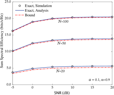
Figure 1: Sum spectral efficiency versus $\mathsf{SNR}$ for different $N(a=0.1$ and $\alpha=0.9)$.

Figure 2: Sum spectral efficiency versus $\alpha$ for different $N(a=0.1$ and $\mathsf{SNR}=0\,$dB).

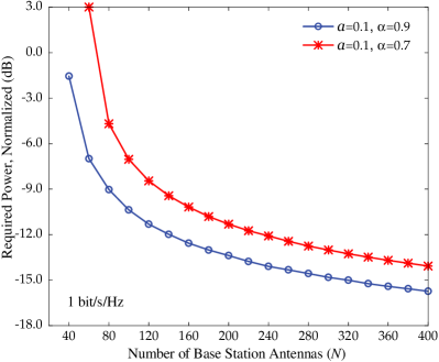
Figure 3: Transmit power required to achieve 1 bit/s/Hz per terminal versus $N(a=0.1$, $\alpha=0.7$ and $\alpha=0.9)$.

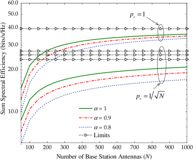
Figure 4: Sum spectral efficiency versus $N$ for different $\alpha$.

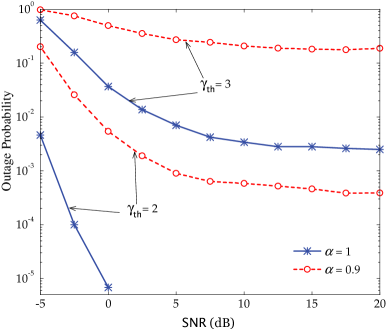
Figure 5: Outage probability versus $\mathsf{SNR}$ for different $\alpha$ and $\gamma_{\tt th}$ ($N=100$).

IV Numerical Results

In this section, we provide numerical results to corroborate our analysis. We deploy a cellular network having $L=7$ cells, each cell has $K=10$ terminals. We choose the frame length is $T=200$ symbols. For each frame, a duration of length $\tau=K$ symbols is used for uplink training. Regarding the large-scale fading coefficients $\beta_{lik}$, we employ a simple model: $\beta_{llk}=1$ and $\beta_{lik}=a$, for $k=1,\ldots,K$, and $i\neq l$. For this simple model, $a$ is considered as an inter-cell interference factor. In all examples, we choose $a=0.1$. Furthermore, we define $\mathsf{SNR}\triangleq p_{r}$.

In the following, we scrutinize the sum-spectral efficiency, defined as:

$$\mathcal{S}_{l}\triangleq\left(1-\frac{\tau}{T}\right)\sum_{k=1}^{K}R_{lk}\left(p_{r},\alpha\right),$$ (42)

where $R_{lk}\left(p_{r},\alpha\right)$ is given in (19).

Figure 1 represents the sum spectral efficiency as a function of SNR for different $N$, with the intercell interference factor $a=0.1$ and the temporal correlation parameter $\alpha=0.9$. The “Exact, Simulation” curves are generated via (13) using Monte-Carlo simulations, the “Exact, Analysis” curves are obtained by using (19), while the “Bound” curves are derived by using the bound formula given in Proposition 2. The exact agreement between the simulated and analytical results validates our analysis and shows that the proposed bound is very tight, especially for a large number of BS antennas. Furthermore, as in the analysis, at high SNR, the sum spectral efficiency saturates. To enhance the system performance, we can add more antennas at the BS. At $\mathsf{SNR}=5$dB, if we increase $N$ from $20$ to $50$ or from $20$ to $100$, then the sum spectral efficiency can be increased by the factors of $2.5$ or $5.5$.

Next, we study the effect of the temporal correlation parameter $\alpha$ on the system performance and examine the tightness of our proposed bound in Proposition 2. Figure 2 shows the sum spectral efficiency versus $\alpha$, for $N=20,50$, and $100$. Here, we choose $\mathsf{SNR}=0$dB. When the temporal correlation parameter decreases (or the time variation of the channel increases), the system performance deteriorates significantly. When $\alpha$ decreases from $1$ to $0.6$, the spectral efficiency is reduced by a factor of $2$. In addition, at low $\alpha$, using more antennas at the BS does not help much in the improvement of the system performance. Regarding the tightness of the proposed bound, we can see that the bound is very tight across the entire temporal correlation range.

Figure 3 depicts the transmit power, $p_{r}$, that is required to obtain $1$ bit/s/Hz per terminal, for $\alpha=0.7$ and $0.9$. As expected, the required transmit power reduces significantly when the number of BS antennas increases. By doubling the number of BS antennas, we can cut back $p_{r}$ by approximately $1.5$ dB. This property is identical to the results of [6].

To further verify our analysis on large antenna limits, we consider Figure 4. Figure 4 shows the sum spectral efficiency versus the number of BS antennas for different values of $\alpha$, and for two cases: the transmit power, $p_{r}$, is fixed regardless of $N$, and the transmit power is scaled as $p_{r}=1/\sqrt{N}$. The “Limits” curves are derived via the results obtained in Section III-C. As expected, as the number of the BS antennas increases, the sum spectral efficiencies converge to their limits. When the transmit power is fixed, the asymptotic performance (as $N\to\infty$) does not depend on the temporal correlation parameter. By contrast, when the transmit power is scaled as $1/\sqrt{N}$, the asymptotic performance depends on $\alpha$.

Finally, we shed light on the outage performance versus SNR at $N=100$, for different temporal correlation parameters ($\alpha=1$, and $0.9$), and for different threshold values ($\gamma_{\tt th}=2$, and $3$). See Figure 5. We can observe that the outage probability strongly depends on $\alpha$. At $\mathsf{SNR}=0$ dB, by reducing $\alpha$ from 1 to $0.9$, the outage probability increases from $7\times 10^{-6}$ to $5\times 10^{-3}$, and from $3\times 10^{-2}$ to $5\times 10^{-1}$ for $\gamma_{\tt th}=2$, and $3$, respectively. In addition, the outage probability significantly improves when the threshold values are slightly reduced. The reason is that, with large antenna arrays, the channel hardening occurs, and hence, the SINR concentrates around its mean. As a result, by slightly reducing the threshold values, we can obtain a very low outage probability.

V Conclusions

This paper analyzed the uplink performance of cellular networks with zero-forcing receivers, coping with the well-known pilot contamination effect and the unavoidable, but less studied, channel aging effect. The latter effect, inherent in the vast majority of practical propagation environments, stems from the terminal mobility. Summarizing the main contributions of this work, new analytical closed-form expressions for the PDF of the SINR and the corresponding achievable ergodic rate that hold for any finite number of BS antennas were derived. Moreover, a complete investigation of the low-SNR regime took place. Nevertheless, asymptotic expressions in the large numbers of antennas/terminals limit were also obtained, as well as the power-scaling law was studied. As a final point, numerical illustrations represented how the channel aging phenomenon affects the system performance for a finite and an infinite number of antennas. Notably, the outcome is that large number of antennas should be preferred even in time-varying conditions.

-A Proof of Proposition 1

By dividing the numerator and denominator of (13) by $\left\|\left[\hat{{\boldsymbol{G}}}_{ll}^{\dagger}[n-1]\right]_{k}\right\|^{2}$, we have

$$\!\!\!\gamma_{k}=\frac{\alpha^{2}p_{r}\left\|\left[\hat{{\boldsymbol{G}}}_{ll}^{\dagger}[n-1]\right]_{k}\right\|^{-2}}{\alpha^{2}p_{r}C\left\|\!\left[\hat{{\boldsymbol{G}}}_{ll}^{\dagger}[n\!-\!1]\right]_{k}\right\|^{-2}\!\!+\!p_{r}\sum_{i=1}^{L}\!\left\|\hat{{\boldsymbol{Y}}}_{i}[n]\right\|^{2}\!+\!1},$$ (43)

where

$$C \triangleq\sum_{i\neq l}^{L}\!\left\|\!\left[\hat{{\boldsymbol{G}}}_{ll}^{\dagger}[n-1]\right]_{k}\!\hat{{\boldsymbol{G}}}_{li}[n-1]\right\|\!=\!\sum_{i\neq l}^{L}\!\left(\!\frac{\beta_{lik}}{\beta_{llk}}\!\right)^{2},$$ (44)

$$\hat{{\boldsymbol{Y}}}_{i}[n] \triangleq\frac{\left[\hat{{\boldsymbol{G}}}_{ll}^{\dagger}[n-1]\right]_{k}\tilde{{\boldsymbol{E}}}_{li}[n]}{\left\|\left[\hat{{\boldsymbol{G}}}_{ll}^{\dagger}[n-1]\right]_{k}\right\|}.$$ (45)

Note that the last equality in (44) follows (5). Since

$$\left\|\left[\hat{{\boldsymbol{G}}}_{ll}^{\dagger}[n-1]\right]_{k}\right\|^{2}=\left[\left(\hat{{\boldsymbol{G}}}_{ll}^{\scriptscriptstyle\mathsf{H}}[n-1]\hat{{\boldsymbol{G}}}_{ll}[n-1]\right)^{-1}\right]_{kk},$$

$\left\|\left[{\boldsymbol{G}}_{ll}^{\dagger}[n-1]\right]_{k}\right\|^{-2}$ has an Erlang distribution with shape parameter $N\!-\!K\!+\!1$ and scale parameter $\hat{\beta}_{llk}$ [20]. Therefore,

$$\left\|\left[\hat{{\boldsymbol{G}}}_{ll}^{\dagger}[n-1]\right]_{k}\right\|^{-2}\mathop{\sim}\limits^{\tt d}X_{k}[n-1].$$ (46)

Furthermore, for a given $\left[\hat{{\boldsymbol{G}}}_{ll}^{\dagger}[n-1]\right]_{k}$, $\hat{{\boldsymbol{Y}}}_{i}[n]$ is a complex Gaussian vector with a zero-mean and covariance matrix $\tilde{{\boldsymbol{D}}}_{li}$ which is independent of $\left[\hat{{\boldsymbol{G}}}_{ll}^{\dagger}[n-1]\right]_{k}$. Thus, $\hat{{\boldsymbol{Y}}}_{i}[n]\sim\mathcal{CN}\left({{\boldsymbol{0}}},{\tilde{{\boldsymbol{D}}}_{li}}\right)$, and is independent of $\left[\hat{{\boldsymbol{G}}}_{ll}^{\dagger}[n-1]\right]_{k}$. As a result, $\sum_{i=1}^{L}\left\|\hat{{\boldsymbol{Y}}}_{i}[n]\right\|^{2}$ is the sum of $KL$ independent but not necessarily identically distributed exponential RVs. From [21, Theorem 2], we have that

$$\sum_{i=l}^{L}\left\|\hat{{\boldsymbol{Y}}}_{i}[n]\right\|^{2}\overset{\tt d}{\sim}Y_{k}[n].$$ (47)

Combining (43)–(47), we arrive at (14) in Proposition 1.

-B Proof of Theorem 1

The achievable uplink ergodic rate of the $k$th terminal in the $l$th cell is given by

$$R_{lk}\!\left(\!p_{r},\alpha\!\right)\!=\!\operatorname{\mathbb{E}}_{{X_{k},Y_{k}\!\!\!}}\left\{{\!\log_{2}\!\!\left(\!\!1\!+\!\frac{p_{r}\alpha^{2}X_{k}[n-1]}{p_{r}\alpha^{2}CX_{k}[n\!-\!1]\!+\!p_{r}Y_{k}[n]\!+\!1}\!\right)}\right\}$$

$$\!=\!\int_{0}^{\infty}\!\!\!\!\int_{0}^{\infty}\!\!\!\log_{2}\left(\!1\!+\!\frac{p_{r}\alpha^{2}x}{p_{r}\alpha^{2}Cx+p_{r}y+1}\!\right)\!p_{{X_{k}}}\left({x}\right)p_{{Y_{k}}}\left({y}\right)dxdy.$$

Using (15) and (16), we obtain

$$R_{lk}\!\left(\!p_{r},\alpha\!\right)=\sum_{p=1}^{\varrho\left(\mathbf{\mathcal{A}}_{k}\right)}\sum_{q=1}^{\tau_{p}\left(\mathbf{\mathcal{A}}_{k}\right)}\!\frac{\mathcal{X}_{p,q}\left(\mathbf{\mathcal{A}}_{k}\right)\mu_{k,p}^{-q}\log_{2}e}{\left(q\!-\!1\right)!\left(N\!-\!K\right)!\hat{\beta}_{llk}^{N-K+1}}$$

$$\!\times\!\!\int_{0}^{\infty}\!\!\!\!\int_{0}^{\infty}\!\!\ln\!\!\left(\!\!1\!+\!\frac{p_{r}\alpha^{2}x}{p_{r}\alpha^{2}Cx\!+\!p_{r}y\!+\!1}\!\right)\!x^{N\!-\!K}e^{\frac{-x}{\hat{\beta}_{llk}}}y^{q-1}e^{\frac{-y}{\mu_{k,p}}}dxdy$$

$$=\sum_{p=1}^{\varrho\left(\mathbf{\mathcal{A}}_{k}\right)}\sum_{q=1}^{\tau_{p}\left(\mathbf{\mathcal{A}}_{k}\right)}\!\frac{\mathcal{X}_{p,q}\left(\mathbf{\mathcal{A}}_{k}\right)\mu_{k,p}^{-q}\log_{2}e}{\left(q\!-\!1\right)!\left(N\!-\!K\right)!\hat{\beta}_{llk}^{N-K+1}}$$

$$\!\times\!\bigg{(}\!\underbrace{\int_{0}^{\infty}\!\!\!\!\!\int_{0}^{\infty}\!\ln\!\!\left(\!1\!+\!\frac{p_{r}\alpha^{2}\left(\!C\!+\!1\!\right)x}{p_{r}y\!+\!1}\!\right)\!x^{N\!-\!K}e^{\frac{-x}{\hat{\beta}_{llk}}}y^{q-1}e^{\frac{-y}{\mu_{k,p}}}dxdy}_{\triangleq\mathcal{I}_{1}}$$

$$\!-\!\!\underbrace{\int_{0}^{\infty}\!\!\int_{0}^{\infty}\!\ln\left(\!1\!+\!\frac{p_{r}\alpha^{2}Cx}{\ p_{r}y\!+\!1}\!\right)\!x^{N\!-\!K}e^{\frac{-x}{\hat{\beta}_{llk}}}y^{q-1}e^{\frac{-y}{\mu_{k,p}}}dxdy}_{\triangleq\mathcal{I}_{2}}\!\!\bigg{)}$$

$$=\sum_{p=1}^{\varrho\left(\mathbf{\mathcal{A}}_{k}\right)}\sum_{q=1}^{\tau_{p}\left(\mathbf{\mathcal{A}}_{k}\right)}\!\frac{\mathcal{X}_{p,q}\left(\mathbf{\mathcal{A}}_{k}\right)\mu_{k,p}^{-q}\log_{2}e}{\left(q\!-\!1\right)!\left(N\!-\!K\right)!\hat{\beta}_{llk}^{N-K+1}}\left(\mathcal{I}_{1}-\mathcal{I}_{2}\right).$$ (48)

We first derive $\mathcal{I}_{1}$ by evaluating the integral over $x$. By using [22, Eq. (4.337.5)], we obtain

$$\mathcal{I}_{1} =\sum_{t=0}^{N-K}\!\int_{0}^{\infty}\!\left[-f(y)^{N-K-t}e^{-f(y)}\mathrm{Ei}\left(f(y)\right)\right.$$

$$\left.+\sum_{u=1}^{N-K-t}\left(u-1\right)!f(y)^{N-K-t-u}\right]y^{q-1}e^{\frac{-y}{\mu_{k,p}}}dy,$$ (49)

where $f(y)\triangleq-\frac{p_{r}y+1}{\hat{\beta}_{llk}p_{r}\alpha^{2}\left(C+1\right)}$. Using [26, Lemma 1] and [24, Eq. (39)], we can easily obtain $\mathcal{I}_{1}$ as given in (III-A). Similarly, we obtain $\mathcal{I}_{2}$ as given in (21). Substitution of $\mathcal{I}_{1}$ and $\mathcal{I}_{2}$ into (48) concludes the proof.

-C Proof of Proposition 2

By using Jensen’s inequality, we have

$$R_{lk}\left(p_{r},\alpha\right) =\operatorname{\mathbb{E}}\left\{{\log_{2}\left(1+\gamma_{k}\right)}\right\}=\operatorname{\mathbb{E}}\left\{{\log_{2}\left(1+\frac{1}{1/\gamma_{k}}\right)}\right\}$$

$$\geq\log_{2}\left(1+\frac{1}{\operatorname{\mathbb{E}}\left\{{1/\gamma_{k}}\right\}}\right)\triangleq R_{L}\left(p_{r},\alpha\right).$$ (50)

To compute $R_{L}\left(p_{r},\alpha\right)$, we need to compute $\operatorname{\mathbb{E}}\left\{{1/\gamma_{k}}\right\}$. From (43), we have

$$\operatorname{\mathbb{E}}\left\{{\frac{1}{\gamma_{k}}}\right\}=C+\frac{1}{\alpha^{2}}\sum_{i=1}^{L}\operatorname{\mathbb{E}}\left\{{\bigg{\|}\left[\hat{{\boldsymbol{G}}}_{ll}^{\dagger}[n-1]\right]_{k}\tilde{{\boldsymbol{E}}}_{li}[n]\bigg{\|}^{2}}\right\}$$

$$\hskip 99.58464pt+\frac{1}{\alpha^{2}p_{r}}\operatorname{\mathbb{E}}\left\{{\bigg{\|}\left[\hat{{\boldsymbol{G}}}_{ll}^{\dagger}[n-1]\right]_{k}\bigg{\|}^{2}}\right\}$$

$$\!=\!C\!+\!\frac{1}{\alpha^{2}}\!\!\operatorname{\mathbb{E}}\left\{{\bigg{\|}\!\!\left[\!\hat{{\boldsymbol{G}}}_{ll}^{\dagger}[n\!-\!1]\!\right]_{k}\!\bigg{\|}^{2}}\right\}\!\!\left(\sum_{i=1}^{L}\!\sum_{k=1}^{K}\!\left(\!\beta_{lik}\!-\!\alpha^{2}\hat{\beta}_{lik}\!\right)\!+\!\frac{1}{p_{r}}\!\right)$$

$$\!=\!C\!+\!\frac{1}{\left(\!N\!-\!K\!\right)\!\alpha^{2}\hat{\beta}_{llk}}\left(\sum_{i=1}^{L}\sum_{k=1}^{K}\!\left(\beta_{lik}\!-\!\alpha^{2}\hat{\beta}_{lik}\!\right)\!+\!\frac{1}{p_{r}}\right).$$ (51)

In the third equality of (51), we have considered the independence between the two variables, while in the last equality, we have used the following result:

$$\operatorname{\mathbb{E}}\left\{{\bigg{\|}\left[\hat{{\boldsymbol{G}}}_{ll}^{\dagger}[n-1]\right]_{k}\bigg{\|}^{2}}\right\}=\operatorname{\mathbb{E}}_{{X_{k}}}\left\{{\frac{1}{X_{k}[n-1]}}\right\}$$

$$\!=\!\int_{0}^{\infty}\!\!\!\frac{e^{-x/\hat{\beta}_{llk}}}{\left(N-K\right)!\hat{\beta}_{llk}^{2}}\!\!\left(\frac{x}{\hat{\beta}_{llk}}\right)^{N\!-\!K\!-\!1}\!\!\!\mathrm{d}x$$

$$=\frac{1}{\left(N-K\right)\hat{\beta}_{llk}}.$$ (52)

Note that we have used [22, Eq. (3.326.2)] to obtain (52). Thus, the desired result (2) is obtained from (-C) and  (51).

-D Proof of Theorem 2

Clearly, from (14), $\gamma_{k}<1/C$. Thus, if $\gamma_{{\tt th}}\geq 1/C$, then $P_{{\tt out}}\left(\gamma_{{\tt th}}\right)=1$. Hence, we focus on the case where $\gamma_{{\tt th}}<1/C$. Taking the probability of the instantaneous SINR $\gamma_{k}$, given by (14), we can determine the outage probability as

$$P_{{\tt out}}\!=\!{\tt Pr}\left(\frac{\alpha^{2}p_{r}X_{k}}{\alpha^{2}p_{r}CX_{k}+p_{r}Y_{k}+1}\leq\gamma_{{\tt th}}\right)$$

$$\!=\!\int_{0}^{\infty}{\tt Pr}\left(X_{k}<\frac{\gamma_{{\tt th}}\left(p_{r}Y_{k}+1\right)}{\alpha^{2}p_{r}-\gamma_{{\tt th}}\alpha^{2}p_{r}C}\left.\right|Y_{k}\right)p_{Y_{k}}(y)\mathrm{d}y$$

$$\!=\!1\!-\!e^{\frac{-\gamma_{{\tt th}}}{p_{r}\bar{\gamma}_{{\tt th}}}}\!\sum^{N-K}_{t=0}\!\!\int_{0}^{\infty}\!\!\!e^{\frac{-y}{\bar{\gamma}_{{\tt th}}}}\!\sum^{N-K}_{t=0}\!\!\frac{\left(\frac{\gamma_{{\tt th}}}{\bar{\gamma}_{{\tt th}}}\right)^{\!\!t}}{t!}\!\left(\!y\!+\!\frac{1}{p_{r}}\!\right)^{\!\!t}\!\!p_{Y_{k}}(y)\mathrm{d}y$$

$$\!=\!1\!-\!e^{\frac{-\gamma_{{\tt th}}}{p_{r}\bar{\gamma}_{{\tt th}}}}\sum_{p=1}^{\varrho\left(\mathbf{\mathcal{A}}_{k}\right)}\sum_{q=1}^{\tau_{p}\left(\mathbf{\mathcal{A}}_{k}\right)}\sum_{t=0}^{N-K}\mathcal{X}_{p,q}\left(\mathbf{\mathcal{A}}_{k}\right)\frac{\mu_{k,p}^{-q}}{\left(q-1\right)}\frac{\left(\frac{\gamma_{{\tt th}}}{\bar{\gamma}_{{\tt th}}}\right)^{t}}{t!}$$

$$\hskip 85.35826pt\times\int_{0}^{\infty}y^{q-1}e^{\frac{-y}{\bar{\gamma}_{{\tt th}})}}\left(y+\frac{1}{p_{r}}\right)^{t}\mathrm{d}y$$

$$\!=\!1\!-\!e^{\frac{-\gamma_{{\tt th}}}{p_{r}\bar{\gamma}_{{\tt th}}}}\!\!\sum_{p=1}^{\varrho\left(\mathbf{\mathcal{A}}_{k}\right)}\!\sum_{q=1}^{\tau_{p}\left(\mathbf{\mathcal{A}}_{k}\right)}\!\sum_{t=0}^{N-K}\!\!\sum_{s=0}^{t}\!\!\binom{t}{s}\mathcal{X}_{p,q}\!\left(\mathbf{\mathcal{A}}_{k}\!\right)\!\frac{\Gamma\left(s\!+\!q\right)\!\bar{\gamma}_{{\tt th}}^{s+q}}{\mu_{k,p}^{q}\left(q\!-\!1\right)},$$ (53)

where $\bar{\gamma}_{{\tt th}}\triangleq\hat{\beta}_{llk}\left(\alpha^{2}-\alpha^{2}C\gamma_{{\tt th}}\right)$, and where in the third equality, we have used that the cumulative density function of $X_{k}$ (Erlang variable) is

$$F_{X_{k}}(x) ={\tt Pr}\left(X_{k}\leq x\right)$$

$$=1-\exp\left(-\frac{x}{\hat{\beta}_{llk}}\right)\sum_{t=0}^{N-K}\frac{1}{t!}\left(\frac{x}{\hat{\beta}_{llk}}\right)^{t}.$$ (54)

The last equality of (53) was derived after applying the binomial expansion of $(y+1/p_{r})^{t}$ and [22, Eq. (3.351.1)].

$$\ddot{R}_{lk}\left(p_{r},\alpha\right)=\frac{1}{\mathrm{ln}2}\operatorname{\mathbb{E}}_{{X_{k},Y_{k}}}\left\{{\frac{\alpha^{2}X_{k}[n-1]\left(\alpha^{4}X_{k}^{2}[n-1]+2\varsigma_{k}\left(1+p_{r}\varsigma_{k}\right)^{2}\left(1+\alpha^{2}p_{r}X_{k}[n-1]+p_{r}\varsigma_{k}\right)\right)}{\left(\alpha^{4}p_{r}^{2}\left(C+1\right)X_{k}^{2}[n-1]+pY_{k}[n]+1\right)^{2}\left(\alpha^{4}p_{r}^{2}CX_{k}^{2}[n-1]+p_{r}Y_{k}[n]+1\right)^{4}}}\right\},$$ (59)

-E Proof of Theorem 3

The initial step for the derivation of the minimum transmit energy per information bit is to cover the need for exact expressions regarding the derivatives of ${R}_{lk}\left(p_{r},\alpha\right)$. In particular, this can be given by

$$\!\!\dot{R}_{lk}\left(\!p_{r},\alpha\!\right)\!=\!\frac{1}{\mathrm{ln}2}$$

$$\!\!\!\!\times\!\operatorname{\mathbb{E}}_{{X_{k},Y_{k}\!\!\!}}\left\{{\!\!\frac{\alpha^{2}X_{k}[n\!-\!1]\big{/}\!\!\left(\!\alpha^{4}p_{r}^{2}CX_{k}^{2}[n\!-\!1]\!+\!p_{r}Y_{k}[n]\!+\!1\!\right)\!\!}{\left(\!\alpha^{4}p_{r}^{2}\left(\!C\!+\!1\!\right)\!X_{k}^{2}[n-1]\!+\!p_{r}Y_{k}[n]+1\!\right)}}\right\}\!\!.$$ (55)

Easily, its value at $p_{r}=0$ is

$$\dot{R}_{lk}\left(0,\alpha\right)=\frac{1}{\mathrm{ln}2}\operatorname{\mathbb{E}}_{{X_{k}}}\left\{{\alpha^{2}X_{k}[n-1]}\right\}.$$ (56)

Aknowledging that $X_{k}[n-1]$ is Erlang distributed, its expectation can be written as

$$\operatorname{\mathbb{E}}_{{X_{k}}}\left\{{X_{k}[n-1]}\right\}=\left(N-K+1\right)\hat{\beta}_{llk}.$$ (57)

Substituting (57) and (56) into (30), we lead to the desired result.

The second derivative of ${R}_{lk}\left(p_{r},\alpha\right)$, needed for the evaluation of the wideband slope, is given by (59) shown at the top of the previous page, where $\varsigma_{k}\triangleq\alpha^{2}CX_{k}[n-1]+Y_{k}[n]$. Hence, $\ddot{R}_{lk}\left(0,\alpha\right)$ can be expressed by

$$\ddot{R}_{lk}\left(0,\alpha\right) =\frac{1}{\mathrm{ln}2}\mathbb{E}_{X_{k},Y_{k}}\left\{\alpha^{6}X_{k}^{3}[n-1]+2\alpha^{4}CX_{k}^{2}[n-1]\right.$$

$$\hskip 71.13188pt\left.+2\alpha^{2}X_{k}[n-1]Y_{k}[n]\right\}.$$ (59)

The moments of $X_{k}[n-1]$ are obtained by means of the corresponding derivatives of its moment generating function (MGF) at zero $\mathrm{M}_{X_{k}}^{\left(n\right)}\left(0\right)$, i.e., $\operatorname{\mathbb{E}}_{{X_{k}}}\left\{{X_{k}^{n}[n-1]}\right\}=\mathrm{M}_{X_{k}}^{\left(n\right)}\left(0\right)$. Thus, having in mind that the MGF of the Erlang distribution is

$$\mathrm{M}_{X_{k}}\left(t\right)=\frac{1}{\left(1-\hat{\beta}_{llk}t\right)^{N-K+1}},$$ (60)

we can obtain the required moments of $X_{k}[n-1]$ as

$$\operatorname{\mathbb{E}}_{{X_{k}}}\left\{{X_{k}^{2}[n-1]}\right\} =\mathrm{M}_{X_{k}}^{\left(2\right)}\left(0\right)$$

$$=\frac{\Gamma\left(N-K+3\right)}{\Gamma\left(N-K+1\right)}\hat{\beta}_{llk}^{2}$$ (61)

$$\operatorname{\mathbb{E}}_{{X_{k}}}\left\{{X_{k}^{3}[n-1]}\right\} =\mathrm{M}_{X_{k}}^{\left(3\right)}\left(0\right)$$

$$=\frac{\Gamma\left(N-K+4\right)}{\Gamma\left(N-K+1\right)}\hat{\beta}_{llk}^{3}.$$ (62)

In addition, since $X_{k}[n-1]$ and $Y_{k}[n]$ are uncorrelated, we have

$$\operatorname{\mathbb{E}}_{{X_{k},Y_{k}}}\left\{{X_{k}[n-1]Y_{k}[n]}\right\}=\operatorname{\mathbb{E}}_{{X_{k}}}\left\{{X_{k}[n-1]}\right\}\operatorname{\mathbb{E}}_{{Y_{k}}}\left\{{Y_{k}[n]}\right\}.$$

In other words, it is necessary to find the expectation of $Y_{k}[n]$. As aforementioned, the PDF of $Y_{k}[n]$ obeys (16) and has expectation given by definition as

$$\operatorname{\mathbb{E}}_{{Y_{k}}}\left\{{Y_{k}[n]}\right\} =\int_{0}^{\infty}yp_{{Y_{k}}}\left({y}\right)\mathrm{d}y$$

$$=\sum_{p=1}^{\varrho\left(\mathbf{\mathcal{A}}_{k}\right)}\sum_{q=1}^{\tau_{p}\left(\mathbf{\mathcal{A}}_{k}\right)}\!\!\mathcal{X}_{p,q}\left(\mathbf{\mathcal{A}}_{k}\right)\frac{\mu_{k,p}^{-q}}{\left(q-1\right)!}\int_{0}^{\infty}\!\!\!y^{q}e^{\frac{-y}{\mu_{k,p}}}\mathrm{d}y$$

$$=\sum_{p=1}^{\varrho\left(\mathbf{\mathcal{A}}_{k}\right)}\sum_{q=1}^{\tau_{p}\left(\mathbf{\mathcal{A}}_{k}\right)}\mathcal{X}_{p,q}\left(\mathbf{\mathcal{A}}_{k}\right)\frac{\mu_{k,p}^{-q}q}{\left(q-1\right)!},$$ (63)

where we have used [22, Eq. (3.326.2)] as well as the identity $\Gamma\left(q+1\right)=q!$. As a result, $\ddot{R}_{lk}\left(0,\alpha\right)$ follows by means of (-E), (62), (63). Finally, substitution of the (56) and (-E) into (31) yields the wideband slope.

References

• [1] A. Papazafeiropoulos, H. Q. Ngo, M. Matthaiou, and T. Ratnarajah, “Uplink performance of conventional and massive MIMO cellular systems with delayed CSIT,” in Proc. IEEE International Symposium on Personal, Indoor and Mobile Radio Communications (PIMRC), Washington, D.C., Sep. 2014.
• [2] “5G: A Technology Vision,” Huawei Technologies Co., Ltd., Shenzhen, China, Whitepaper, Nov. 2013. [Online]. www.huawei.com/ilink/en/download/HW_314849
• [3] D. Gesbert, M. Kountouris, R. W. Heath Jr., C. B. Chae, and T. Sälzer, “Shifting the MIMO paradigm,” IEEE Sig. Proc. Mag., vol. 24, no. 5, pp. 36–46, Oct. 2007.
• [4] T. L. Marzetta, “Noncooperative cellular wireless with unlimited numbers of base station antennas,” IEEE Trans. Wireless Commun., vol. 9, no. 11, pp. 3590–3600, Nov. 2010.
• [5] E. G. Larsson, F. Tufvesson, O. Edfors, and T. L. Marzetta, “Massive MIMO for next generation wireless systems,” IEEE Commun. Mag., vol. 52, no. 2, pp. 186–195, Feb. 2014.
• [6] H. Q. Ngo, E. G. Larsson, and T. L. Marzetta, “Energy and spectral efficiency of very large multiuser MIMO systems,” IEEE Trans. Commun., vol. 61, no. 4, pp. 1436–1449, Apr. 2013.
• [7] H. Li, L. Song, and M. Debbah, “Energy efficiency of large-scale multiple antenna systems with transmit antenna selection,” IEEE Trans. Commun., vol. 62, no. 2, pp. 638–647, Feb. 2014.
• [8] C. J. Chen and L. C. Wang, “Performance analysis of scheduling in multiuser MIMO systems with zero-forcing receivers,” IEEE J. Sel. Areas Commun., vol. 25, no. 7, pp. 1435–1445, Sep. 2007.
• [9] G. Caire and S. Shamai (Shitz), “On the achievable throughput of a multiantenna Gaussian broadcast channel,” IEEE Trans. Inf. Theory, vol. 49, no. 7, pp. 1691–1706, Jul. 2006.
• [10] H. Q. Ngo, M. Matthaiou, T. Q. Duong, and E. G. Larsson, “Uplink performance analysis of multicell MU-SIMO systems with ZF receivers,” IEEE Trans. Veh. Tech., vol. 62, no. 9, pp. 4471–4483, Nov. 2013.
• [11] J. Jose, A. Ashikhmin, T. L. Marzetta, and S. Vishwanath, “Pilot contamination and precoding in multi-cell TDD systems,” IEEE Trans. Wireless Commun., vol. 10, no. 8, pp. 2640–2651, Aug. 2011.
• [12] K. E. Baddour and N. C. Beaulieu, “Autoregressive modelling for fading channel simulation,” IEEE Trans. Wireless Commun., vol. 4, no. 4, pp. 1650–1662, July 2005.
• [13] K. T. Truong and R. W. Heath, Jr., “Effects of channel aging in Massive MIMO Systems,” IEEE/KICS J. Commun. Netw., vol. 15, no. 4, pp. 338–351, Aug. 2013.
• [14] V. Pohl, P. H. Nguyen, V. Jungnickel, and C. V. Helmolt, “Continuous flat-fading MIMO channels: Achievable rate and optimal length of the training and data phases,” IEEE Trans. Wireless Commun., vol. 4, no. 4, pp. 1889-1900, July 2005.
• [15] A. Papazafeiropoulos and T. Ratnarajah “Uplink performance of massive MIMO subject to delayed CSIT and anticipated channel prediction,” in Proc. IEEE ICASSP, May 2014.
• [16] C. Kong, C. Zhong, A.K. Papazafeiropoulos, M. Matthaiou and Z. Zhang “Sum-Rate and Power Scaling of Massive MIMO Systems with Channel Aging” IEEE Trans. on Commun., vol. 63, no. 12, pp. 4879–4893, 2015.
• [17] A. K. Papazafeiropoulos and T. Ratnarajah “Deterministic Equivalent Performance Analysis of Time-Varying Massive MIMO Systems,” IEEE Trans. of Wireless Commun., vol.14, no.10, pp.5795-5809, Oct. 2015.
• [18] A. K. Papazafeiropoulos, “Impact of General Channel Aging Conditions on the Downlink Performance of Massive MIMO,” IEEE Transactions on Vehicular Technology, 2016, to appear.
• [19] H. Shin and M. Z. Win, “MIMO diversity in the presence of double scattering,” IEEE Trans. Inf. Theory, vol. 54, no. 7, pp. 2976–2996, Jul. 2008.
• [20] D. A. Gore, R. W. Heath Jr., and A. J. Paulraj, “Transmit selection in spatial multiplexing systems,” IEEE Commun. Lett., vol. 6, no. 11, pp. 491–493, Nov. 2002.
• [21] A. Bletsas, H. Shin, and M. Z. Win, “Cooperative communications with outage-optimal opportunistic relaying,” IEEE Trans. Wireless Commun., vol. 6, no. 9, pp. 3450–3460, Sep. 2007.
• [22] I. S. Gradshteyn and I. M. Ryzhik, Table of Integrals, Series, and Products, 7th ed.   San Diego, CA: Academic, 2007.
• [23] Wolfram, “The Wolfram functions site.” Available: http://functions.wolfram.com
• [24] M. Kang and M.-S. Alouini, “Capacity of MIMO Rician channels,” IEEE Trans. Wireless Commun., vol. 5, no. 1, pp. 112–122, Jan. 2006.
• [25] A. P. Prudnikov, Y. A. Brychkov, and O. I. Marichev, Integrals and Series, Volume 3: More Special Functions.   New York: Gordon and Breach Science, 1990.
• [26] H. Q. Ngo, T. Q. Duong, and E. G. Larsson, “Uplink performance analysis of multicell MU-MIMO with zero-forcing receivers and perfect CSI,” in Proc. IEEE Swe-CTW, Sweden, Nov. 2011.
• [27] S. Verdú, “Spectral effciency in the wideband regime,” IEEE Trans. Info. Theory, vol. 48, no. 6, pp. 1319–1343, Jun. 2002.
• [28] P. Billingsley, Probability and Measure, 3rd ed. John Wiley & Sons, Inc., 1995.
• [29] A. W. van der Vaart, Asymptotic Statistics (Cambridge Series in Statistical and Probabilistic Mathematics). Cambridge University Press, New York, 2000.
• [30] S. Shamai (Shitz) and S. Verdú, “The impact of frequency-flat fading on the spectral efficiency of CDMA,” IEEE Trans. Inf. Theory, vol. 47, no. 4, pp. 1302–1327, May 2001.
• [31] A. Lozano, A. M. Tulino, and S. Verdú, “High–SNR power offset in multiantenna communications,” IEEE Trans. Inf. Theory, vol. 51, no. 12, pp. 4134–4151, Dec. 2005.