Testing theories of Gravity and Supergravity with inflation and observations of the cosmic microwave background

Abstract

Cosmological and astrophysical observations lead to the emerging picture of a universe that is spatially flat and presently undertaking an accelerated expansion. The observations supporting this picture come from a range of measurements encompassing estimates of galaxy cluster masses, the Hubble diagram derived from type-Ia supernovae observations, the measurements of Cosmic Microwave Background radiation anisotropies, etc. The present accelerated expansion of the universe can be explained by admitting the existence of a cosmic fluid, with negative pressure. In the simplest scenario this unknown component of the universe, the Dark Energy, is represented by the cosmological constant ($\Lambda$), and accounts for about 70% of the global energy budget of the universe. The remaining 30% consists of a small fraction of baryons (4%) with the rest cold Dark Matter (CDM). The Lambda Cold Dark Matter ($\Lambda$CDM) model, i.e. General Relativity with cosmological constant, is in good agreement with observations. It can be assumed as the first step towards a new standard cosmological model. However, despite the satisfying agreement with observations, the $\Lambda$CDM model presents several lacks of congruence and shortcomings, and therefore theories beyond Einstein’s General Relativity are called for. Many extensions of Einstein’s theory of gravity have been studied and proposed with various motivations like the quest for a quantum theory of gravity to extensions of anomalies in observations at the solar system, galactic and cosmological scales. These extensions include adding higher powers of Ricci curvature $R$, coupling the Ricci curvature with scalar fields and generalized functions of $R$. In addition when viewed from the perspective of Supergravity (SUGRA) many of these theories may originate from the same SUGRA theory, but interpreted in different frames. SUGRA therefore serves as a good framework for organizing and generalizing theories of gravity beyond General Relativity. All these theories when applied to inflation (a rapid expansion of early Universe in which primordial gravitational waves might be generated and might still be detectable by the imprint they left or by the ripples that persist today) can have distinct signatures in the Cosmic Microwave Background radiation temperature and polarization anisotropies. We give a review of $\Lambda$CDM cosmology and survey the theories of gravity beyond Einstein’s General Relativity, specially which arise from SUGRA, and study the consequences of these theories in the context of inflation and put bounds on the theories and the parameters therein from the observational experiments like PLANCK, Keck/BICEP etc. The possibility of testing these theories in the near future in CMB observations and new data coming from colliders like the LHC, provides an unique opportunity for constructing verifiable models of particle physics and General Relativity.

1 Introduction

The attempt to find a consistent quantum theory of gravity has motivated attempts to find generalizations of Einsteins General Theory of Relativity. The recent cosmological observations, in fact, suggest that the present Universe is in accelerating phase accUn . To explain such a behavior one is forced to introduce the concept of Dark Energy. Moreover, for explaining the rotation curves of Galaxies one needs to introduce Dark Matter. The origin and nature of both Dark Energy (DE) and Dark Matter (DM), that undoubtedly represent a fundamental issue in particle physics, astrophysics and cosmology, is unknown and although many attempts have been done to explain such dark components, no final conclusions has been reached, and the question till now is completely open.

Observations of the cosmic microwave background anisotropy motivate the idea that the universe in the past went through a period of accelerated expansion called inflation. The specific model of inflation which fits the temperature and polarization anisotropies is still not settled. It’s not established yet whether inflation requires a fundamental scalar field in a particle physics model or whether the scalar degrees of freedom of the metric in modified gravity theories can give rise to viable inflation. In this review we survey the generailised theories of gravity which can give inflation compatible with observations of the CMB by experiments like Planck Ade:2015lrj ; Planck:2015 and BICEP2/Keck+Planck BKP:2015 ; bicep2keck2015 ; Ade:2015xua .

General features of metric theories of gravity

In order that a theory of gravity might be considered a valid theory, it must fulfill some minimal requirements: $1)$ It must reproduce the Newtonian dynamics in the weak-energy limit, which means that it has to pass the classical Solar System tests which are all experimentally well founded Will93 . $2)$ It must reproduce Galactic dynamics in relation to the observed baryonic constituents (hence luminous components as stars, or planets, dust and gas), radiation and Newtonian potential which is, by assumption, extrapolated to Galactic scales. $3)$ It must address the problem of large scale structure and the cosmological dynamics. General Relativity (GR) is the simplest theory that satisfies these requirements. It is based on the assumption that space and time are entangled into a single space-time structure, which must reduce to Minkowski’s space-time structure in absence of gravitational forces. GR underlies also on Riemann’s ideas according to which the Universe is a curved manifold riemann and that the distribution of matter affects point by point the local curvature of the space-time structure.

GR is strongly based on some assumptions that the Physics of Gravitation has to satisfy:

The Principle of Relativity: All frames are good frames for describing Physics. This implies that no preferred inertial frame should be chosen a priori (if any exists).

The Principle of Equivalence: Inertial effects are locally indistinguishable from gravitational effects (i.e. the equivalence between the inertial and the gravitational mass).

The Principle of General Covariance: Field equations are generally covariant.

The Principle of Causality: Each point of space-time should admit a universally valid notion of past, present and future.

On the basis of the above principles, Einstein postulates that the gravitational forces must be related to the curvature of a metric tensor field $ds^{2}=g_{\mu\nu}dx^{\mu}dx^{\nu}$ defined on a four-dimensional space-time manifold (the metric signature is the same of Minkowski’s metric, $(-,+,+,+)$) and that space-time is curved, with the curvature locally determined by the distribution of the sources, the latter described by the energy-momentum tensor $T^{(m)}_{\mu\nu}$. An important achievement was to prove that the field equations for a metric tensor $g_{\mu\nu}$ can be obtained by starting from an action linearly depending on Ricci’s scalar $R$ (Hilbert-Einstein action schroedinger .)

$$S_{HE}=\frac{1}{2\kappa^{2}}\int d^{4}x\sqrt{-g}\,R+S_{matter}\,,\qquad\kappa^{2}=8\pi G/c^{4}\,.$$ (1.1)

The choice of Hilbert and Einstein was completely arbitrary, but it was certainly the simplest one. Some years later the GR formulation, it was clarified by Levi–Civita that curvature is not a purely metric notion. It is indeed related to the linear connection, which plays a central role in the definition of parallel transport and covariant derivation levicivita (this is, in some sense, the precursor idea of what would be called a ”gauge theoretical framework” gauge , after the Cartan work cartan ). As later clarified, the principles of relativity, equivalence and covariance require that the space-time structure has to be determined by either one or both of two fields: a metric $g$ and a linear connection $\Gamma$ (symmetric in order that the theory is torsionless). The metric $g$ fixes the causal structure of space-time (the light cones) as well as some metric relations (clocks and rods); the connection $\Gamma$ fixes the free-fall, i.e. the locally inertial observers. They have to satisfy a number of compatibility relations, which generally lead to a specific form of the connection in terms of the metric tensor (Levi-Civita connections), but they can be also independent, leading to the Palatini approach of GR. palatiniorigin . It is on this basis that the so-called alternative theories of gravitation, or Extended Theories of Gravitation (ETGs) arise. In fact their starting points is that gravitation is described by either a metric (purely metric theories), or by a linear connection (purely affine theories) or by both fields (metric-affine theories). Here the Lagrangian is a scalar density of the curvature invariants, constructed by mean of $\{g,\Gamma\}$.

Attempts to generalize GR along these lines unification and investigations about ”alternative theories” continued even after 1960 Will93 . What arises from these studies is that the search for a coherent quantum theory of gravitation or the belief that gravity has to be considered as a sort of low-energy limit of string theories green , has renew the idea that there is no reason to follow the simple prescription of Einstein and Hilbert. Other curvature invariants or non-linear functions of them should be also considered, especially in view of the fact that they have to be included in both the semi-classical expansion of a quantum Lagrangian or in the low-energy limit of a string Lagrangian.

Not only from a mathematical point of view there is the necessity to generalize GR, but also current astrophysical and cosmological observations suggest that, as already pointed out, Einstein’s equations are no longer a good test for gravitation at Galactic, extra-galactic and cosmic scales, unless one does not admit that the matter side of field equations contains some kind of exotic matter-energy which is the dark matter and dark energy side of the Universe.

One can adopt a different point of view, in the sense that instead of changing the matter side of Einstein field equations to fit the missing matter-energy content of the currently observed Universe (by adding any sort of exotic matter and/or energy), one may change the gravitational side of the equations, admitting corrections coming from non-linearities in the effective Lagrangian. This is a possibility that needs to explored, even if, without a complete theory of gravity, one has to tune up the form of effective theory that is going to study, hence a huge family of allowed Lagrangians can be chosen, trying to fit all possible observational tests, at all scales (Solar, Galactic, extragalactic and cosmic, and so on).

1.1 Shortcomings in the standard cosmological model

We shortly review the shortcomings of the cosmological standard model (the cosmology based on GR) or hot Big Bang. The latter provides a framework for the description the evolution of the Universe. The spacetime evolution is governed by Einstein’s field equation (which contains matter content of the Universe)

$$R_{\mu\nu}-\frac{1}{2}g_{\mu\nu}R+\Lambda g_{\mu\nu}={\kappa}^{2}T_{\mu\nu}\,,$$ (1.2)

This equation follows by varying the action (1.1) with respect to the metric $g_{\mu\nu}$, while

$$T_{\mu\nu}=-\frac{2}{\sqrt{-g}}\frac{\delta S_{matter}}{\delta g_{\mu\nu}}$$

is the energy-momentum tensor. $\Lambda$ is the cosmological constant (it enters into (1.1) by replacing $R\to R+\Lambda$).

There are three important epochs to which the early Universe undergoes: radiation, matter and vacuum (energy) domination eras. They are characterized by an appropriate relation between pressure and energy density of matter, $p=p(\rho)$. Assuming the homogeneity and isotropy of the (flat) cosmological background Friedman-Robertson-Walker (FRW) Universe, the line element is given by

$$ds^{2}=-dt^{2}+a^{2}(t)d{\bf x}^{2}\,,$$ (1.4)

where $a(t)$ is the scale factor. For a long time, the success of the Big Bang model was based on three cornerstones: $i)$ Hubble expansion, $ii)$ the distribution of relic photons (CMBR), and $iii)$ the light element abundance such as ${}^{3}He$, ${}^{4}He$, $D$, ${}^{7}Li$ (Big Bang Nucleosynthesis (BBN)). With the recent developments of modern Cosmology, our view of the Universe evolution has been completely transformed. For example, the cosmological model present some inconsistencies that can be solved only admitting the existence of the Inflation, i.e. a period of accelerated expansion of the Universe which occurred in the very early phase of the Universe evolution. It is believed that Inflation is responsible for the inhomogeneities in the matter distribution (whose evolution allowed the formation of structures, stars, planets) and the inhomogeneities of the CMB. These perturbations are generated by quantum fluctuations of the scalar field (the inflaton) which drives the Inflation, and they can be scalar, vectorial or tensorial. The challenge of modern cosmology is to verify all predictions of Inflationary scenario.

The Inflationary paradigm allows to solve some inconsistence of the standard cosmological model:

• Flatness of the Universe - $\Omega=\rho/\rho_{c}=1$ where $\rho=3H^{2}m_{P}^{2}/8\pi$ is the critical density. Without Inflation, the adjustment of $\Omega$ should be $\sim 10^{-60}$ at the Planck era, and $\sim 10^{-15}$ at the primordial nucleosynthesis.

• The problems of homogeneity, isotropy, and horizon (which created headache in the frameworks of FRW cosmology) are elegantly solved.

• Inflation provides a natural mechanism of generation of small density perturbations with practically flat spectrum in agreement with observations.

• To solve all problems of standard FRW cosmology, the duration of Inflation must be $N=Ht\sim 70-100$.

We will return on the standard cosmological model and Inflation in next Sections.

2 FRW Cosmology - Inflation

Today the very basic picture of our observable universe is presented quite accurately by the standard Big Bang model of cosmology, also known as $\Lambda CDM$-model or FLRW cosmology. Under the standard Big Bang model, the universe in its early stages is considered to be very hot, uniform in its density and expanding uniformly in all the directions and cooling down at late times. So far, it has passed a large number of increasingly precise tests. It successfully predicts the age, Hubble expansion rate, mass density of the universe and light elemental abundance in the early universe. Also it explains the presence of the Cosmic Microwave Background Radiation (CMBR). The CMBR is a snapshot of the oldest light in our universe leftover after decoupling and imprinted on the Last Scattering Surface (LSS), when the universe was just $3,80,000$ years old. The most remarkable feature of CMBR is its high degree of uniformity everywhere and in all the directions. It has inhomogeneity only at the level of one part in $10^{5}$. These tiny inhomogeneities in the early universe are believed to have grown to cosmological scales later in the history of the universe which resulted in structure formation: stars, galaxies and galactic clusters of today. Current precision measurements of these small inhomogeneities in the CMBR has led to constraining a variety of cosmological parameters and therefore theoretical cosmological models. However, the standard Big Bang model could poorly explain some of the observed characteristics of the universe, $e.g.$ why the universe is so uniform and its intrinsic geometry is so flat. These unsolved problems in standard cosmological model are also known as Horizon and Flatness problems. Invocation of a rapid exponential expansion phase, Inflation, in the very beginning of the universe could solve these problems.

In the standard model of cosmology, the matter content of the universe is described by a perfect fluid which is characterised only by the energy density $\rho$ and isotropic pressure $p$. The stress-energy-momentum tensor for a perfect fluid with energy density $\rho$ and pressure $p$ is given by

$$T_{\mu\nu}=(\rho+p)u_{\mu}u_{\nu}+pg_{\mu\nu},$$ (2.1)

where $u_{\mu}$ is the 4-velocity of the fluid in some arbitrary coordinate system $x_{\mu}$ given by $u_{\mu}=\frac{dx_{\mu}}{d\tau}$. Here $\tau$ is the proper time of the observer, so that $g^{\mu\nu}u_{\mu}u_{\nu}=-1$. If such a fluid is at rest in the geometry described by metric (1.4) and obeys the equation of state $p_{i}=\omega_{i}\rho_{i}$, then from the covariant conservation of the stress-energy-momentum tensor ($\bigtriangledown_{\mu}T^{\mu\nu}=0$) one finds the equation of motion of energy densities in the FLRW universe

$$\dot{\rho}_{i}+3H(1+\omega_{i})\rho_{i}=0,$$ (2.2)

where $H=\frac{\dot{a}}{a}$ is the Hubble parameter describing Hubble expansion rate, $i$ represents the various components of the cosmological fluid, $e.g.$ matter, radiation and dark energy, and $\omega_{i}$ represents the respective equation of state parameter for different components. For the system as a whole, the total energy density is given by

$$\rho=\sum_{i}\rho_{i}\,,$$

and total pressure by

$$p=\sum_{i}p_{i}\,.$$

The solution of the continuity equation (2.2) is given by

$$\rho_{i}\propto a^{-3(1+\omega_{i})}.$$ (2.3)

As the universe expands, the matter density, consisting of all non-relativistic matter particles, dilutes as $\rho_{nr}\propto a^{-3}$; and radiation density, consisting of all relativistic particles, dilutes as $\rho_{r}\propto a^{-4}$, as for pressureless non-relativistic matter $\omega=0$ and for radiation $\omega=\frac{1}{3}$. For $\omega=-1$ which corresponds to a negative pressure fluid, a strange behavior occurs, the energy density of the universe remains constant as the universe expands. Such an exotic matter is known as Dark Energy or Cosmological Constant and usually attributed to the present day accelerated expansion of our universe.

In the flat FLRW universe the dynamics of the scale factor $a(t)$ is determined through Friedmann equations which can be derived by solving Einstein field equation for the FLRW metric (1.4) and energy-momentum tensor (2.1)

$$\frac{\dot{a}^{2}}{a^{2}} = \frac{8\pi G\rho}{3}+\frac{\Lambda}{3}-\frac{\kappa}{a^{2}},$$ (2.4)

$$\frac{\ddot{a}}{a} = -\frac{4\pi G}{3}(\rho+3p)+\frac{\Lambda}{3},$$ (2.5)

According to acceleration equation if $\Lambda=0$ then the matter and radiation filled universe decelerates which contradicts the observational data from Type-1a supernovae accUn , South Pole Telescope Story:2012wx and from the measurement of high multipole CMB data Smoot:1998jt ; WMAP9 ; Planck:2015 . These observations have led to the conclusion that the universe is accelerating in its expansion. In the $\Lambda CDM$ model the present accelerated expansion is achieved with a small positive cosmological constant $\Lambda$. Also Eq. (2.5) implies that the present accelerated expansion can be achieved if the energy density of the universe is dominated by some unknown exotic matter with negative pressure $p<-\frac{\rho}{3}$ or equation of state parameter $\omega<\frac{-1}{3}$, which generates repulsive gravity. To consider different matter contributions to the total energy density of the universe, it is common to define the density parameter as

$$\Omega_{i}\equiv\frac{\rho_{i}}{\rho_{c}}$$ (2.6)

where $\rho_{c}$ is the critical density for which the universe is spatially flat $i.e.$ from equation (2.4) $\rho_{c}=\frac{3H^{2}}{8\pi G}$ for $\kappa=0$. We define the total density parameter of the universe as

$$\Omega=\sum_{i}\Omega_{i}\,.$$

If we divide Friedmann equation (2.4) by $H^{2}$, it can be written as

$$\sum_{i}\Omega_{i}+\Omega_{\kappa}=\Omega_{m}+\Omega_{r}+\Omega_{\Lambda}+\Omega_{\kappa}=1$$ (2.7)

where

$$\Omega_{\Lambda}=\frac{\Lambda}{3H^{2}}=\frac{8\pi G}{3H^{2}}\rho_{\Lambda}$$

and

$$\Omega_{\kappa}=-\frac{\kappa}{H^{2}a^{2}}$$

are the dark energy and curvature density parameters respectively. The matter density parameter consists of baryonic matter and non-relativistic cold dark matter (CDM), $i.e.$

$$\Omega_{m}=\Omega_{b}+\Omega_{CDM}\,.$$

The recent Planck observations of CMB Planck:2015 combined with WMAP polarization data WMAP9 for low multipoles $l<23$, give the present values of the density parameters at $68\%CL$ as:

$$\Omega_{b}h^{2} = 0.02205\pm 0.00028,$$ (2.8)

$$\Omega_{CDM}h^{2} = 0.1199\pm 0.0027,$$ (2.9)

$$\Omega_{\Lambda} = 0.685^{+0.018}_{-0.016},$$ (2.10)

where $h$ is the dimensionless parameter defined through the present value of the Hubble parameter as

$$H_{0}=100h~{}km~{}s^{-1}Mpc^{-1}=67.3\pm 1.2~{}km~{}s^{-1}Mpc^{-1}\,.$$

Therefore, the present observations suggest that our universe is composed of nearly $4.9\%$ atoms (or baryons), $26.8\%$ (cold) dark matter and $68.3\%$ of dark energy which adds up to approximately $1$ in the total density parameter. According to Planck combined with BAO data Planck:2015

$$\Omega_{\kappa}=0.000\pm 0.005~{}~{}(95\%~{}CL)\,,$$ (2.11)

i.e., the observations suggest that the intrinsic geometry of our universe is (very close to) flat $i.e.$ $\kappa\simeq 0$ or the universe is at the critical density. Why the universe is so close to flat geometry or at its critical density is known as flatness problem.

2.1 Inflation

We have seen that the $\Lambda CDM$ model can describe the evolution of the universe in a great detail. Before we discuss the mathematical description of inflation, let us briefly discuss the problem of initial conditions. The conventional model of standard Big Bang cosmology requires a set of fine-tuned initial conditions so that the universe could evolve to its present state. These initial conditions are the assumptions of the extreme flatness and homogeneity in the beginning of the universe. The dramatic flatness of the universe at its beginning can not be predicted or explained by the standard model, instead it must be assumed as an initial condition. Similarly, the large scale homogeneity of the universe is not predicted or explained by the standard model but it must be assumed.

In the late 1970’s, cosmologists realised the problem of initial conditions with the $\Lambda CDM$ model and solution to these problems could be reached at with the invocation of Inflation, i.e. an accelerated expansion phase in the early evolution of the universe Guth:1980zm The cosmological inflation is believed to took place in the very early universe around $10^{-35}$ seconds after the Big Bang. Remarkably, inflation not only explains the large scale homogeneity and isotropy of the universe but also widely accepted as responsible for the formation and evolution of the structures in the universe. Inflation can provide the mechanism for producing the tiny density fluctuations which are responsible for seeding the structures in our universe $e.g.$ stars, galaxies and galactic clusters.

Mathematically, the accelerated expansion of the FLRW universe or condition for inflation can be given as

$$\ddot{a}>0.$$ (2.12)

The second time derivative of the scale factor can easily be related to the time variation of the Hubble parameter as

$$\frac{\ddot{a}}{a}=H^{2}(1-\epsilon),$$ (2.13)

where $\epsilon\equiv-\frac{\dot{H}}{H^{2}}$. Therefore acceleration $\ddot{a}>0$ corresponds to

$$\epsilon=-\frac{\dot{H}}{H^{2}}=-\frac{1}{H}\frac{dH}{dN}<1,$$ (2.14)

here, we have defined $dN$ as

$$dN=d\ln a=Hdt\,,$$

which determines the number of e-foldings in an inflationary expansion. More precisely the number of e-foldings $N$ during inflation in the time interval $t_{i}<t<t_{e}$ is given by the integral

$$N=\int_{t_{i}}^{t_{e}}Hdt.$$ (2.15)

The equation (2.14) implies that the fractional change in the Hubble parameter per e-folding is small. An inflationary scenario where this change is too small $i.e.$ $\epsilon<<1$ is termed as slow-roll inflation. From the acceleration equation (2.5), we see that, for inflation, the energy density of the universe must be dominated by a fluid whose equation of state satisfies the condition

$$\omega\equiv\frac{p}{\rho}<-\frac{1}{3}.$$ (2.16)

2.2 Scalar Fields as a Source of Inflation

The existence of scalar fields in the very early universe is suggested by our best theories of fundamental interactions in Nature, which predict that the universe went through a succession of phase transitions in its early stages as it expanded and cooled. In general, the phase transition occurs when certain scalar parameters known as Higgs fields acquire a non-zero value or vacuum expectation value (VEV) via a process called spontaneous symmetry breaking. The symmetry is manifest as long as the Higgs fields have not acquired vev and it is spontaneously broken as soon as at least one of the Higgs fields become non-zero. Therefore, the existence of scalar fields in the early universe is suggested by the occurrence of phase transitions and therefore provides the motivation for considering them as the source of inflation (it can act as a negative pressure source). The simplest inflation models involves a single scalar field $\phi$ which in the inflationary context is termed as inflaton. The model is described by the following action

$$S = \int d^{4}x\sqrt{-g}\left[-\frac{M_{p}^{2}}{2}R+\frac{1}{2}g^{\mu\nu}\partial_{\mu}\phi\partial_{\nu}\phi+V(\phi)\right]$$ (2.17)

$$= \int d^{4}x\sqrt{-g}\left(\mathcal{L}_{EH}+\mathcal{L}_{\phi}\right)\,.$$ (2.18)

In this action the inflaton field has a minimal coupling with the gravity and a canonical kinetic term. $V(\phi)$ is the potential of the field due to self-interaction and it can be different in different inflation models. Here we will assume an arbitrary $V(\phi)$. We shall set $M_{p}=1$, restore it at the end of caluctions. The energy momentum tensor of the scalar field is

$$T_{\mu\nu}^{\phi}=\partial_{\mu}\phi\partial_{\nu}\phi-g_{\mu\nu}\left[\frac{1}{2}\partial^{\rho}\phi\partial_{\rho}\phi+V(\phi)\right].$$ (2.19)

In principle, scalar fields can be dependent on space and time both $i.e.$ $\phi=\phi(t,{\bf x})$, however as we know that the universe is homogeneous on largest scales, therefore at the background level, homogeneity implies that scalar field can be described by its time dependence only, $i.e.$ $\phi(t,{\bf x})\equiv\phi(t)$. Therefore for the homogeneous background field, the energy momentum tensor for $\phi$ takes the form of a perfect fluid (2.1) with energy density and pressure for scalar fields given by

$$\rho_{\phi} = \frac{\dot{\phi}^{2}}{2}+V(\phi),$$ (2.20)

$$p_{\phi} = \frac{\dot{\phi}^{2}}{2}-V(\phi)\,.$$ (2.21)

The resulting equation of state is

$$\omega_{\phi}\equiv\frac{p_{\phi}}{\rho_{\phi}}=\frac{\frac{\dot{\phi}^{2}}{2}-V(\phi)}{\frac{\dot{\phi}^{2}}{2}+V(\phi)}.$$ (2.22)

If the potential energy of the field dominates over its kinetic energy $i.e.$ $\dot{\phi}^{2}<<V(\phi)$, then the above simple relation (2.22) implies that the scalar field can act as a negative pressure source $i.e.$ $\omega_{\phi}<0$ and can provide accelerated expansion $i.e.$ $\omega_{\phi}<-\frac{1}{3}$ (see (2.16)). The Friedmann equation and the equation of motion of the scalar field are

$$H^{2} = \frac{1}{3}\left(\frac{\dot{\phi}^{2}}{2}+V(\phi)\right)\,,$$ (2.23)

$$\ddot{\phi} + 3H\dot{\phi}+V^{\prime}(\phi)=0\,.$$ (2.24)

These equations determine the dynamics of the space and scalar field in a FRW universe.

2.2.1 Slow-roll Inflation

The equations (2.24) and (2.23) can be solved analytically for some specific potentials $V(\phi)$, however in general, an analytical solution is possible only under slow-roll approximation. As discussed above, slow-roll inflation occurs when $\dot{\phi}^{2}\ll V(\phi)$ which implies that the field $\phi$ rolls down the potential slow enough that the potential is nearly constant during inflation. A second order differentiation of the condition $\dot{\phi}^{2}\ll V(\phi)$ implies $\ddot{\phi}\ll V^{\prime}(\phi)$ which ensures that the accelerated expansion is sustained for a sufficient period of time. Under slow-roll approximation equations (2.24) and (2.23) become

$$3H\dot{\phi} \simeq -V^{\prime}(\phi),$$ (2.25)

$$3H^{2} \simeq V(\phi).$$ (2.26)

It is worth noting that the time variation of the Hubble parameter and scalar field can be related easily by differentiating equation (2.26) w.r.t. time and combining the result with Eq. (2.25) as

$$\dot{H}\simeq-\frac{\dot{\phi}^{2}}{2}.$$ (2.27)

The slow-roll conditions $\dot{\phi}^{2}\ll V(\phi)$ and $\ddot{\phi}\ll V^{\prime}(\phi)$ can be put into useful dimensionless parameters as

$$\epsilon = -\frac{\dot{H}}{H^{2}}\simeq\frac{1}{2}\left(\frac{V^{\prime}(\phi)}{V(\phi)}\right)^{2}\ll 1,$$ (2.28)

$$\eta = -\frac{\ddot{\phi}}{H\dot{\phi}}\simeq\frac{V^{\prime\prime}(\phi)}{V(\phi)}\ll 1.$$ (2.29)

These two conditions ensures that the potential $V(\phi)$ is sufficiently ‘flat’ that the field $\phi$ rolls slowly enough for inflation to occur. After the end of inflation when field has crossed the flat part of the potential, it fast rolls, $\dot{\phi}^{2}\approx V(\phi)$, towards the minimum of the potential and then oscillates and decays into the standard model particles.

It is worth considering the case in which $V(\phi)$ is nearly constant during some part of the period of inflation during which Hubble expansion is constant. Solving (2.26), one obtains that during this period scale factor evolves exponentially $a(t)\sim e^{Ht}$, such a spacetime is approximately de-Sitter. From the acceleration equation (2.13), it is clear that inflation ends when $\epsilon(\phi_{e})=1$, which represents the violation of slow-roll condition $\epsilon\ll 1$ and as soon as this condition is met $i.e.$ $\epsilon=1$, the kinetic energy of the field $\dot{\phi}^{2}$ becomes comparable to its potential energy $V(\phi)$ and the potential becomes steeper and field speeds up towards the minimum of the potential. The number of e-foldings before the inflation ends, as defined in (2.28), is given by (see (2.15))

$$N(\phi) = \int_{t_{i}}^{t_{e}}Hdt$$

$$= \int_{\phi_{i}}^{\phi_{e}}\frac{H}{\dot{\phi}}d\phi\simeq\int_{\phi_{e}}^{\phi_{i}}\frac{V}{V^{\prime}}d\phi\,,$$

where we used the slow-roll equations (2.25) and (2.26). To solve the horizon and flatness problems it is required that the total number of e-foldings during inflation exceeds $60$

$$N_{tot}\equiv\ln\frac{a_{e}}{a_{i}}\gtrsim 60.$$ (2.31)

However the precise value of $N_{tot}$ depends on the energy scale of inflation and details of the reheating after inflation. It is during the slow-roll phase, which lasts nearly $40-60$ e-folds before inflation ends (the precise value again is determined by the details of reheating and post-inflationary evolution of the universe), when the quantum fluctuations in the field are imprinted on the CMB and $\phi_{i}$ corresponds to the field value when these fluctuations in the CMB are created.

2.3 Inflation models and key inflationary observables

The models of inflation can be broadly divided into two categories: large field inflation and small field inflation. The class of models in which during inflation $\phi_{s}>1M_{p}$ are called the large field models. The chaotic potential $V(\phi)=\lambda_{n}\phi^{n}$ models and exponential potential $V(\phi)=V_{0}e^{\phi}$ models are the large field type models. In the chaotic inflation scenario, first introduced in Linde:1983gd , as the universe exits the Planck era at $t\sim 10^{-43}sec$ the initial value of the inflaton field is set chaotically, $i.e.$ it acquires different values in different parts of the universe and the initial displacement of the field from the minimum of the potential is larger than Planck scale. These models usually satisfy $V^{\prime\prime}(\phi)>0$. The small field inflation models, instead are characterized by the fact that the slow-roll trajectory is at the small field values $\phi_{s}<1M_{p}$. In these models the field starts close to an unstable maximum of the potential and rolls down to a stable minimum. An example of small field models is ’new inflation’ Linde:1981mu which arises naturally in the mechanism of spontaneous symmetry breaking. In general, the form of the potential in these models are $V(\phi)=V_{0}(1-\phi^{n})$ and typically these models satisfy $V^{\prime\prime}(\phi)<0$.

A basic difference between the large field and small field models is that the large field models predict large amplitude of gravity waves produced during inflation whereas the small field models predict small amplitudes of gravity waves which are too small to be detected in future observations. In either class of these models the inflation ends as soon as the slow-roll conditions are violated and the field rolls down to the minimum of the potential, oscillates and decays into the standard model particles. The decay process of the fields into standard model particles is known as reheating and after this universe eventually enters into the radiation domination phase Bassett:2005xm ; Allahverdi:2010xz .

The models of standard slow-roll inflation are typically defined through its scalar potential. For any inflation model in order not to be ruled out, it must predict certain physical quantities in agreement with the observations. These physical quantities/observables are: the amplitude of the power spectrum of curvature perturbations $\Delta_{\mathcal{R}}^{2}$, spectral index $n_{s}$, running of spectral index $\alpha_{s}$ and tensor-to-scalar ratio $r$. The latest constraints on the inflationary observables as given by Planck-2015, for the combination Planck TT $+$ lowP, are Ade:2015lrj

$$\ln(10^{10}\Delta_{\mathcal{R}}^{2}) = 3.089\pm 0.036,$$ (2.32)

$$n_{s} = 0.9666\pm 0.0062,$$ (2.33)

$$r_{0.002} < 0.1.$$ (2.34)

The above values are for 7-parameter $\Lambda CDM$+$r$ model, when there is no scale dependence of the scalar and tensor spectral indices. The value of amplitude and spectral index are given at $68\%CL$ at the pivot scale $k=0.05Mpc^{-1}$. Whereas the upper bound on tensor-to-scalar ratio is determined at $95\%CL$ at $k=0.002Mpc^{-1}$  Ade:2015lrj . There are numerous models of inflation. For a review on variety of models of inflation we refer the reader to ref. Martin:2013tda and references therein.

Also for 8-parameter $\Lambda CDM$+$r$+$\alpha_{s}$ model, when there is $k-$dependence of the spectral index or there is a running of the spectral index, the Planck observations give

$$n_{s} = 0.9667\pm 0.0132,$$ (2.35)

$$r_{0.05} < 0.168.$$ (2.36)

The value of amplitude and spectral index are given at $68\%CL$ at the pivot scale $k=0.05Mpc^{-1}$. Whereas the upper bound on tensor-to-scalar ratio is determined at $95\%CL$ at $k=0.05Mpc^{-1}$. However, the amplitude of the power spectrum remains the same. Notice that with running, the constraint on tensor-to-scalar ratio is relaxed.

Later, the joint BICEP2/Keck Array and Planck analysis put an upper limit on tensor-to-scalar BKP:2015

$$r_{0.05}<0.12~{}~{}~{}~{}~{}~{}at~{}~{}95\%CL.$$ (2.37)

Most recently BICEP2/Keck Array Collaboration with its CMB polarization data and combining it with Planck analysis of CMB polarization and temperature data have further improved the bound on $r$ bicep2keck2015 ; Ade:2015xua

$$r_{0.05}<0.07~{}~{}~{}~{}~{}~{}at~{}~{}95\%CL.$$ (2.38)

We will use these observed values to constrain parameters of the models studied in this review.

3 Cosmological Perturbation Theory

Here we present the calculation of the primordial density fluctuations power spectra generated by quantum fluctuations in the inflaton field during inflation. Observation of the CMB anisotropies $\frac{\delta\rho}{\rho}\sim 10^{-5}$ proves that the early universe was not perfectly uniform in its matter distribution. However, as the observed anisotropies are very small, therefore these can be analyzed in terms of linear quantum fluctuations $\delta\phi(t,{\bf x})$ around the homogeneous background. The linear theory of cosmological perturbations is a cornerstone of the modern cosmology. It not only explains the CMB anisotropies but also the formation and evolution of the structures in the universe. The seed of these anisotropies were stretched to astronomical scales because of the superluminal expansion of the cosmic space during inflationary quasi de-Sitter expansion. This theory has been extensively studied in literature; the details can be found in Ref.s Baumann:2009ds ; Riotto:2002yw .

The linear perturbations of the metric $g_{\mu\nu}$ can be decomposed according to their spin w.r.t. a local rotation of the spatial coordinates on the hypersurfaces of constant time into three kinds of perturbations: scalar, vector and tensor. Here we will study only scalar and tensor perturbations in detail. Scalar perturbations explain the CMB temperature anisotropy (or matter density fluctuations) and the seed for the structure formations in the universe. One can see from the Einstein field equation (1.2) (with $\Lambda=0$) that the scalar perturbations which give rise to perturbations in the energy-momentum tensor leads to metric perturbations. On the other hand, metric perturbations back react through the perturbations in the KG equations of motion (2.24) of the field, giving rise to field (or matter) perturbations. Therefore

$$\delta g_{\mu\nu}(t,{\bf x})\Longleftrightarrow\delta\phi(t,{\bf x})\,.$$ (3.39)

The tensor perturbations corresponds to primordial gravitational waves which is a generic prediction of inflationary models. Observational constraints on the amplitude of the primordial gravitational waves can be used to eliminate various inflation models.

3.1 Linear Perturbations

Linear order perturbations in the metric and field around the homogeneous background solutions of the field $\phi(t)$ and the metric $g_{\mu\nu}(t)$ can be given as

$$\delta\phi(t,{\bf x}) = \phi(t,{\bf x})-\phi(t),$$ (3.40)

$$\delta g_{\mu\nu}(t,{\bf x}) = g_{\mu\nu}(t,{\bf x})-g_{\mu\nu}(t).$$ (3.41)

The most general linearly perturbed spatially flat FRW metric can be written as

$$ds^{2}=-(1+2\Phi)dt^{2}+2a(t)B_{i}dtdx^{i}+a(t)^{2}\left[(1-2\Psi)\delta_{ij}+2E_{ij}\right]dx^{i}dx^{j},$$ (3.42)

where $\Phi,\Psi$ are the scalar perturbations, $B_{i}$ are the vector perturbations and $E_{ij}$ are the tensor perturbations. According to SVT decomposition scalar, vector and tensor perturbations are decoupled during inflation and therefore evolve independently, this is also known as Decomposition Theorem. This theorem implies that if some physical process in the early universe sets up tensor perturbations then these do not induce scalar perturbations, on the other hand, evolution of the scalar perturbations is unaffected by the presence of any possible vector and tensor perturbations dodelson . The importance of SVT decomposition is that the Einstein equations for scalar, vector and tensor perturbations do not mix at linear order and can therefore be studied separately. In this way the SVT decomposition greatly simplifies the calculations. The vector perturbations are not sourced by inflation and furthermore they quickly decay with the expansion of the universe Baumann:2009ds . Therefore we will ignore vector perturbations and focus on scalar and tensor perturbations only.

According to SVT decomposition of the metric perturbations in real space, the vector $B_{i}$ can be decomposed into a gradient of as scalar, say $B$, and divergence free vector, say $S_{i}$, as

$$B_{i}\equiv\partial_{i}B-S_{i},\quad\quad\text{where}\quad\partial^{i}S_{i}=0,$$ (3.43)

and similarly, any second rank tensor $E_{ij}$ can be written in terms of a divergence free vector and a traceless and divergence free tensor as

$$E_{ij}\equiv 2\partial_{i}\partial_{j}E+2\partial_{(i}F_{j)}+h_{ij}\,,$$ (3.44)

where

$$\partial^{i}F_{i}=0,\quad h_{i}^{i}=\partial^{i}h_{ij}=0\,.$$

Since the $g_{\mu\nu}$ is a symmetric tensor therefore in $4$-dimensions it has $10$ independent components or $10$ degrees of freedom (d.o.f.). The $10$ d.o.f. of metric has been decomposed into $4+4+2$ SVT d.o.f., $i.e.$ $4$ scalar d.o.f. $\Psi,\Phi,B,E$, $2$ vector d.o.f. for $S_{i},F_{i}$ vectors each and $2$ d.o.f. of tensor $h_{ij}$.

3.2 Gauge Transformation and Gauge Invariance

In GR the gauge transformations are the general coordinate transformations from one local reference frame to another. Here we will briefly review the gauge fixing and the behavior of the scalar, vector and tensor perturbations under general coordinate transformation. We will introduce the gauge invariant quantities in next Section. Fixing a gauge in GR implies choosing a coordinate system, a slicing of spacetime into constant time hypersurfaces and threading into lines with fixed spatial coordinate ${\bf x}$. Now let us consider the infinitesimal coordinate transformations

$$x^{\mu}\rightarrow\tilde{x}^{\mu}=x^{\mu}+\xi^{\mu}\,,$$

where $\xi^{\mu}$ is a spacetime dependent infinitesimal quantity. At a given point on spacetime manifolds, the metric in the new coordinate system $\tilde{x}^{\mu}$ can be determined using the invariance of the line-element

$$ds^{2}=g_{\mu\nu}dx^{\mu}dx^{\nu}=\tilde{g}_{\mu\nu}d\tilde{x}^{\mu}d\tilde{x}^{\nu}\,,$$

or by applying the usual tensor transformation law

$$\tilde{g}_{\mu\nu}(\tilde{x}^{\rho})=\frac{\partial x^{\mu}}{\partial\tilde{x}^{\alpha}}\frac{\partial x^{\nu}}{\partial\tilde{x}^{\beta}}g_{\mu\nu}(x^{\rho}).$$ (3.45)

Consider splitting the metric $g_{\mu\nu}(x^{\rho})$ into background and perturbed parts in both $x^{\mu}$ and $\tilde{x}^{\mu}$ coordinate systems

$$g_{\mu\nu}(x^{\rho}) = g^{(0)}_{\mu\nu}(x^{\rho})+\delta g_{\mu\nu}(x^{\rho}),$$ (3.46)

$$\tilde{g}_{\mu\nu}(\tilde{x}^{\rho}) = g^{(0)}_{\mu\nu}(\tilde{x}^{\rho})+\delta\tilde{g}_{\mu\nu}(\tilde{x}^{\rho}).$$ (3.47)

Note that we have not put tilde over the background metric because due to homogeneity and isotropy, the background forms of the metric tensor (also vectors and scalars) does not change, so that the background quantities behave the same way in the new coordinate system $\tilde{x}^{\mu}$. Partial differentiation of coordinate transformations gives

$$\frac{\partial x^{\mu}}{\partial\tilde{x}^{\alpha}}=\delta^{\mu\alpha}-\frac{\partial\xi^{\mu}}{\partial\tilde{x}^{\alpha}}\,.$$

The background metric can be expanded as

$$g^{(0)}_{\mu\nu}(x^{\rho})=g^{(0)}_{\mu\nu}(\tilde{x}^{\rho}-\xi^{\rho})\simeq g^{(0)}_{\mu\nu}(\tilde{x}^{\rho})-\frac{\partial g^{(0)}_{\alpha\beta}}{\partial\tilde{x}^{\rho}}\xi^{\rho}.$$ (3.48)

Substituting (3.46) into (3.45) and comparing with (3.46) while using (3.48), one infers the transformation law of metric tensor perturbation,

$$\delta g_{\alpha\beta}(x^{\rho})\rightarrow\delta\tilde{g}_{\alpha\beta}(\tilde{x}^{\rho})=\delta g_{\alpha\beta}-\frac{\partial g^{(0)}_{\alpha\beta}(\tilde{x}^{\rho})}{\partial\tilde{x}^{\rho}}\xi^{\rho}-g^{(0)}_{\alpha\nu}(x^{\rho})\frac{\partial\xi^{\nu}}{\partial\tilde{x}^{\beta}}-g^{(0)}_{\mu\beta}(x^{\rho})\frac{\partial\xi^{\mu}}{\partial\tilde{x}^{\alpha}}.$$ (3.49)

Similarly, for a $4-$vector $u^{\mu}(x^{\rho})$ which transform as

$$\tilde{u}_{\alpha}(\tilde{x}^{\rho})=\frac{\partial x^{\mu}}{\partial\tilde{x}^{\alpha}}u_{\mu}(x^{\rho})\,,$$

one obtains that its perturbation $\delta u_{\alpha}(x^{\rho})=u_{\alpha}(x^{\rho})-u^{(0)}_{\alpha}(x^{\rho})$ transforms as

$$\delta u_{\alpha}(x^{\rho})\rightarrow\delta\tilde{u}_{\alpha}(\tilde{x}^{\rho})=\delta u_{\alpha}(x^{\rho})-\frac{\partial u^{(0)}_{\alpha}(\tilde{x}^{\rho})}{\partial\tilde{x}^{\rho}}\xi^{\rho}-u^{(0)}_{\mu}(x^{\rho})\frac{\partial\xi^{\mu}}{\partial\tilde{x}^{\alpha}},$$ (3.50)

while, for a scalar $q(x^{\mu})$, which doesn’t change under the coordinate transformation

$$\tilde{q}(\tilde{x}^{\mu})=q(x^{\mu})\,,$$

one gets that its perturbation $\delta q(x^{\mu})=q(x^{\mu})-q^{(0)}(x^{\mu})$ transforms as

$$\delta q(x^{\mu})\rightarrow\delta\tilde{q}(\tilde{x}^{\mu})=\delta q(x^{\mu})-\frac{\partial q^{(0)}(\tilde{x}^{\rho})}{\partial\tilde{x}^{\rho}}\xi^{\rho}.$$ (3.51)

Let us now write the temporal and spatial components of the infinitesimal vector $x^{\mu}\rightarrow\tilde{x}^{\mu}=x^{\mu}+\xi^{\mu}$ as

$$t\rightarrow t+\alpha,\qquad x^{i}\rightarrow x^{i}+\delta^{ij}\partial_{j}\beta\,,$$ (3.52)

where

$$x^{\mu}\equiv(x^{0},x^{i})=(t,x^{i})\,,\quad\xi^{\mu}\equiv(\xi^{0},\xi^{i})=(\alpha,\partial^{i}\beta)\,.$$

$\alpha$ is infinitesimal temporal shift and $\beta$ is a scalar function. Using the metric tensor and scalar perturbation transformation laws (3.49) and (3.51), we find that the tensor perturbations $h_{ij}$ are invariant under the gauge transformations (and therefore they already represents gravitational waves in a gauge invariant manner), whereas the scalar perturbations $\Phi$, $\Psi$, $B$ and $E$ transform as

$$\Phi \rightarrow \Phi-\dot{\alpha},$$

$$\Psi \rightarrow \Psi+H\alpha,$$

$$B \rightarrow B+a^{-1}\alpha-a\dot{\beta},$$

$$E \rightarrow E-\beta,$$ (3.53)

Thus we find that only $\alpha$ and $\beta$ contributes to the transformations of the scalar perturbations and we can choose them appropriately (as we are free to choose them) and can impose two conditions on the scalar functions $\Phi$, $\Psi$, $B$ and $E$ to remove any two of them. This is called the gauge fixing or gauge choice which corresponds to choosing a gauge transformation. It is possible that the freedom in coordinate choice leads to an appearance of fictitious perturbation modes which do not describe any real physical inhomogeneities. However, one can construct gauge invariant quantities which do not depend on choice of coordinate system and represents real inhomogeneities. Two important gauge-invariant quantities were introduced by Bardeen Bardeen:1980kt

$$\Phi_{B} \equiv \Phi-\frac{d}{dt}[a^{2}(\dot{E}-B/a)],$$ (3.54)

$$\Psi_{B} \equiv \Psi+a^{2}H(\dot{E}-B/a).$$ (3.55)

The gauge invariance of $\Phi_{B}$ and $\Psi_{B}$ implies that if they vanish in one particular coordinate system then they will be vanishing in any coordinate system. Such a construction of gauge invariant quantities allows us to distinguish between physical inhomogeneities and fictitious perturbations. If there are metric perturbations present even when both $\Phi_{B}$ and $\Psi_{B}$ are zero, then they are fictitious perturbations and can be eliminated using change of coordinates.

Using (3.51), we find that the perturbations of the scalar field $\phi$ transform as

$$\delta\tilde{\phi}(\tilde{x}^{\mu})=\delta\phi(x^{\mu})-\frac{\partial\phi^{(0)}(x^{\rho})}{\partial x^{\rho}}\xi^{\rho}.$$ (3.56)

Since the background field $\phi^{(0)}=\phi(t)$ is time-dependent only, therefore

$$\delta\tilde{\phi}(\tilde{x}^{\mu})=\delta\phi(x^{\mu})-\dot{\phi}(t)\alpha,$$ (3.57)

where $\alpha=\xi^{0}$. Also the matter perturbations or the perturbations to the total stress energy tensor $T_{\mu\nu}$ are given in terms of the perturbations of the energy density $\delta\rho$, perturbations of pressure $\delta p$ and perturbations of momentum density $\delta q$. Under gauge transformation these perturbations transform as

$$\delta\rho \rightarrow \delta\rho-\dot{\rho}\alpha,$$

$$\delta p \rightarrow \delta p-\dot{p}\alpha,$$

$$\delta q \rightarrow \delta q+(\rho+p)\alpha.$$ (3.58)

3.3 Gauge Invariant Variables

We discussed and explained the fictitious and real perturbations in previous Section. In order to avoid the fictitious gauge modes, it is preferable to use the gauge-invariant combinations of the matter and metric perturbations Bardeen:1980kt . An important gauge-invariant quantity is the comoving curvature perturbation $\mathcal{R}$ Bardeen:1983qw defined as

$$\mathcal{R}\equiv\Psi-\frac{H}{\rho+p}\delta q,$$ (3.59)

this can also be given in terms of the metric perturbations in the longitudinal gauge as Mukhanov:1990me

$$\mathcal{R}=\Psi-\frac{H}{\dot{H}}(\dot{\Psi}+H\Phi),$$ (3.60)

and for perfect fluid, this can further be simplified to give (we use $\Psi=\Phi$, see Eq. (3.88))

$$\mathcal{R}=\Phi-\frac{H}{\dot{H}}(\dot{\Phi}+H\Phi).$$ (3.61)

The condition (3.59) can be constructed by considering the slicing of the spacetime into constant $\delta q$ (or constant-$\phi$) hyperserfaces which provide the constraint

$$\delta q\rightarrow\delta q+(\rho+p)\alpha=0\quad\Longrightarrow\quad\alpha=-\frac{\delta q}{\rho+p}$$ (3.62)

substituting this $\alpha$ into the metric transformation relation $\Psi\rightarrow\Psi+H\alpha$ gives the relation (3.59) for $\mathcal{R}$. Since $\delta q$ is the scalar $0i-$component of the perturbed energy momentum tensor $T_{i}^{0}=\partial_{i}\delta q$ and during inflation $T^{0}_{i}=-\dot{\phi}\partial_{i}\delta\phi$, therefore both of these relations implies $\delta q=-\dot{\phi}\delta\phi$. Also from (2.20) we have $\rho+p=\dot{\phi}^{2}$. Then the comoving curvature perturbations (3.59) during inflation becomes

$$\mathcal{R}\simeq\Psi+\frac{H}{\dot{\phi}}\delta\phi\,.$$ (3.63)

Geometrical interpretation of $\mathcal{R}$ is that it measures the spatial curvature of the comoving hypersurface where $\delta\phi=0$, $i.e.$

$$\mathcal{R}=\Psi|_{\delta\phi=0}.$$ (3.64)

Another important gauge-invariant quantity is curvature perturbations on constant energy density hypersurfaces $\mathcal{\zeta}$ defined as

$$-\mathcal{\zeta}\equiv\Psi+\frac{H}{\dot{\rho}}\delta\rho\,,$$ (3.65)

Similar to $\mathcal{R}$, the quantity $\mathcal{\zeta}$ can be constructed by considering the slicing of the spacetime into constant energy density hyperserfaces which provide the constraint

$$\delta\rho\rightarrow\delta\rho-\dot{\rho}\alpha=0\quad\Longrightarrow\quad\alpha=\frac{\delta\rho}{\dot{\rho}}$$ (3.66)

substituting this $\alpha$ into the metric transformation relation $\Psi\rightarrow\Psi+H\alpha$ gives the relation (3.65) for $\mathcal{\zeta}$. Since during slow-roll (from equation (2.20)) one has

$$\delta\rho=\dot{\phi}\delta\dot{\phi}+V^{\prime}\delta\phi\simeq V^{\prime}\delta\phi$$

and

$$\dot{\rho}=\dot{\phi}\ddot{\phi}+V^{\prime}\dot{\phi}\simeq V^{\prime}\dot{\phi}\,.$$

These equations implies

$$\frac{\delta\rho}{\dot{\rho}}\simeq\frac{\delta\phi}{\dot{\phi}}\,.$$

As a consequence, $-\zeta$ becomes

$$-\mathcal{\zeta}\simeq\Psi+\frac{H}{\dot{\phi}}\delta\phi.$$ (3.67)

Geometrical interpretation of $\mathcal{\zeta}$ is that it measures the spatial curvature of the uniform density hypersurface, $i.e.$

$$-\mathcal{\zeta}=\Psi|_{\delta\rho=0}.$$ (3.68)

We see that the curvature perturbations $\mathcal{R}$ and $\mathcal{\zeta}$ by construction are invariant under the gauge transformations (3.52), which can be verified using (3.53) and (3.58) into their expressions (3.59) and (3.65).

Also using the linearized Einstein field equations it can be shown that the gauge invariant curvature perturbations $\mathcal{\zeta}$ and $\mathcal{R}$ are related as Baumann:2009ds

$$-\zeta=\mathcal{R}+\left(\frac{k}{aH}\right)^{2}\frac{2\rho}{3(\rho+p)}\Psi_{B},$$ (3.69)

which implies that on superhorizon scale $k\ll aH$, $\mathcal{\zeta}$ and $\mathcal{R}$ are equal. Also we saw that under slow-roll they are equal, $cf.$ equations (3.63) and (3.67). We conclude that:

The curvature perturbations $\mathcal{\zeta}$ and $\mathcal{R}$ also share an important property that on superhorizon scales they are conserved for adiabatic matter perturbations.

In general, it is possible that the pressure perturbations (in any gauge) can be split into adiabatic and non-adiabatic (entropic) parts as

$$\delta p \equiv \delta p_{ad}+\delta p_{nad}$$ (3.70)

$$= c_{s}^{2}\delta\rho+\delta p_{nad}\,,$$ (3.71)

where $c_{s}^{2}\equiv\frac{\dot{p}}{\dot{\rho}}$ and the adiabatic pressure perturbations are defined as

$$\delta p_{ad}\equiv\frac{\dot{p}}{\dot{\rho}}\delta\rho\,.$$ (3.72)

They satisfy the condition

$$\frac{\delta p}{\dot{p}}=\frac{\delta\rho}{\dot{\rho}}$$ (3.73)

which implies that a given time displacement $\delta t$ causes the same relative fractional change $\frac{\delta X}{\dot{X}}$ in all scalar quantities $X\equiv(\rho,p,...)$. The non-adiabatic part of the pressure perturbations $\delta p_{nad}$ are defined as

$$\delta p_{nad}\equiv\dot{p}\Gamma\equiv\delta p-\frac{\dot{p}}{\dot{\rho}}\delta\rho\,,$$ (3.74)

where

$$\Gamma\equiv\frac{\delta p}{\dot{p}}-\frac{\delta\rho}{\dot{\rho}},$$ (3.75)

is the entropy perturbation, also known as isocurvature perturbation. $\Gamma$, defined in this way, is gauge-invariant and represents the displacement between hypersurfaces of uniform pressure and uniform density.

Using the perturbed Einstein field equations (3.80), as discussed in detail in the next Section, it can be shown that the evolution of the gauge invariant curvature perturbations in the longitudinal gauge is given by Kaiser:2010yu ; Baumann:2009ds

$$\mathcal{\dot{R}}=-\frac{H}{\rho+p}\delta p_{nad}+\left(\frac{k}{aH}\right)^{2}\left[\frac{H^{2}}{3(\rho+p)}\delta q\right],$$ (3.76)

therefore if there are no non-adiabatic matter perturbations $\delta p_{nad}=0$ or no isocurvature perturbations $\Gamma=0$, the curvature perturbations $\mathcal{R}$ (also $\mathcal{\zeta}$, $cf.$ equation (3.69)) are conserved on superhorizon scales $k\ll aH$.

Physical Interpretation of Adiabatic (Curvature) and Isocurvature perturbations: If the curvature perturbations are such that they can not give rise to variations in the relative density between different components of the cosmological fluid (photons, baryons, neutrinos and CDM particles) after inflation, then the curvature perturbations are adiabatic :

$$\delta\left(\frac{n_{m}}{n_{r}}\right)=0\quad\Longrightarrow\quad\frac{\delta n_{m}}{n_{m}}=\frac{\delta n_{r}}{n_{r}},$$ (3.77)

where

$$\delta n=n(t,{\bf x})-n^{(0)}(t)$$

and the index $m$ collectively stands for non-relativistic matter components $e.g.$ baryons and CDM and index $r$ for relativistic matter components $e.g.$ photons and neutrinos. Since

$$n_{(m,r)}\propto a^{-3}\,,\quad\rho_{m}\propto a^{-3}\,,\quad\rho_{r}\propto a^{-4}\,,$$

the condition (3.77) gives

$$\frac{\delta\rho_{m}}{\rho_{m}}=\frac{3}{4}\frac{\delta\rho_{r}}{\rho_{r}}.$$ (3.78)

In single-field slow inflationary scenario, the condition (3.78) holds and therefore the perturbations produced by single-field inflation are purely adiabatic. However, in inflationary models with more than one field, the perturbations are not necessarily adiabatic. If during inflation there are more than one field and all are evolving in time, the fluctuations orthogonal to background trajectory can affect the relative density between different components of the cosmological fluid even if the total density (and therefore spatial curvature) is unperturbed Gordon:2000hv . For example, the relative density perturbations (isocurvature/entropy perturbations) between photon and CDM can be defined as

$$\Gamma_{m\gamma}\equiv\frac{\delta\rho_{cdm}}{\rho_{cdm}}-\frac{3}{4}\frac{\delta\rho_{\gamma}}{\rho_{\gamma}}.$$ (3.79)

Since adiabatic and isocurvature perturbations give different peak structure in the CMB power spectrum, therefore different type of perturbations can be distinguished from the CMB measurements. In fact, CMB observations suggest that even if the isocurvature perturbations are present, their amplitude is vanishingly small compared to amplitude of the adiabatic (curvature) perturbations Ade:2015lrj . The theoretical predictions of the isocurvature perturbations are extremely model dependent. Not only the presence of more than one scalar field may give rise to entropic perturbations but these may also be generated in non-minimally coupled inflation models Kaiser:2010yu . Also the post-inflationary evolution may generate them.

3.4 Curvature Perturbation and Scalar Power Spectrum

For a metric with small perturbations, the Einstein tensor $G_{\nu\mu}$ can be written as

$$G_{\nu\mu}=G^{(0)}_{\nu\mu}+\delta G_{\nu\mu}+....\,,$$

where $\delta G_{\nu\mu}$ represents the terms with linear metric perturbations $\delta g_{\mu\nu}$. The stress energy tensor $T^{\nu}_{\mu}$ can be split in a similar fashion and we get the linearized Einstein field equations

$$\delta G^{\nu}_{\mu}=8\pi G~{}\delta T^{\nu}_{\mu}.$$ (3.80)

The gauge freedom allows to choose the two functions $\alpha$ and $\beta$ which provides two conditions on the scalar functions $\Phi$, $\Psi$, $B$, $E$ and therefore allows to remove any two of them. The gauge freedom greatly simplifies the calculations and knowing the solutions of the gauge-invariant variables, one can calculate the density and metric perturbations in any coordinate system in a simple way mukhanov . One of many useful gauges is the conformal Newtonian gauge or longitudinal gauge which is defined by the conditions

$$B=0\,,\quad E=0\,.$$

In this gauge the FRW line element assumes the simple form

$$ds^{2}=-(1+2\Phi)dt^{2}+a(t)^{2}(1-2\Psi)\delta_{ij}dx^{i}dx^{j}.$$ (3.81)

Now we calculate the perturbed Einstein field equations (3.80). For the metric (3.81), the components of the perturbed Einstein tensor can be obtained as

$$\delta G^{0}_{0} = -2\nabla^{2}\Psi+6H^{2}\Phi+6H\dot{\Psi},$$ (3.82)

$$\delta G^{0}_{i} = -2\partial_{i}(H\Phi+\dot{\Psi}),$$ (3.83)

$$\delta G^{i}_{j} = \partial^{i}\partial_{j}(\Psi-\Phi)+[\nabla^{2}(\Phi-\Psi)+2\ddot{\Psi}+(4\dot{H}+6H^{2})\Phi+H(2\dot{\Phi}+2\dot{\Psi})]\delta^{i}_{j}.$$ (3.84)

Using the perfect fluid description as defined in equation (2.1) and the stress-energy-momentum tensor for the scalar field $\phi$ as defined in equation (2.19), the components of the perturbed $T_{\mu\nu}$ are given by

$$\delta T^{0}_{0} = -\delta\rho=\dot{\phi}^{2}\Phi-\dot{\phi}\delta\dot{\phi}-V^{\prime}\delta\phi,$$ (3.85)

$$\delta T^{0}_{i} = \delta q=-\dot{\phi}\partial_{i}\delta\phi,$$ (3.86)

$$\delta T^{i}_{j} = \delta p=[-\dot{\phi}^{2}\Phi+\dot{\phi}\delta\dot{\phi}-V^{\prime}\delta\phi]\delta^{i}_{j}.$$ (3.87)

where the relation

$$\delta T^{\nu}_{\mu}=\delta(g^{\nu\tau}T_{\mu\tau})=\delta g^{\nu\tau}T_{\mu\tau}+g^{\nu\tau}\delta T_{\mu\tau}$$

has been used. To compute the curvature perturbation $\mathcal{R}$, one first considers the $ij$-component of the perturbed Einstein field equation (3.80). From equation (3.87), we see that the stress energy tensor has no off-diagonal components, therefore taking the off-diagonal components, $i.e.$ $i\neq j$, of the equations (3.84) and (3.87), we have

$$\partial^{i}\partial_{j}(\Psi-\Phi)=0\quad\Longrightarrow\quad\Phi=\Psi,$$ (3.88)

therefore we can work with any of the variable $\Phi$ or $\Psi$, let’s work with $\Psi$. We note that if the spatial part of the stress energy tensor is diagonal, $i.e.$ $\delta T^{i}_{j}\propto\delta^{i}_{j}$, the variable $\Phi$ or $\Psi$ can be seen as a generalisation of the Newtonian potential which therefore explains the name Newtonian gauge for this choice of coordinate system. Considering the diagonal components, $i.e.$ $i=j$, of equations (3.84) and (3.87), one gets

$$\ddot{\Psi}+4H\dot{\Psi}+(2\dot{H}+3H^{2})\Psi=-\dot{\phi}^{2}\Phi+\dot{\phi}\delta\dot{\phi}-V^{\prime}\delta\phi.$$ (3.89)

Since $\phi$ is background quantity which is only time dependent, therefore equations (3.83) and (3.86) for $0i$-components give

$$\dot{\Psi}+H\Psi=4\pi G~{}\dot{\phi}\delta\phi=\epsilon H^{2}\frac{\delta\phi}{\dot{\phi}},$$ (3.90)

where $\epsilon=4\pi G\frac{\dot{\phi}^{2}}{H^{2}}$ (slow-roll parameter). Similarly the equations (3.82) and (3.85) for $00$-component gives

$$\nabla^{2}\Psi-3H\dot{\Psi}-3H^{2}\Psi=4\pi G(\dot{\phi}\delta\dot{\phi}-\dot{\phi}^{2}\Psi+V^{\prime}\delta\phi).$$ (3.91)

For the purpose of analysis, it is convenient to work in terms of the Fourier decomposition of the metric and the field perturbations, and see what happens to a perturbation corresponding to a given comoving spatial scale $k$ with corresponding comoving wavelength $\lambda=\frac{2\pi}{k}$. Using Fourier transformation, we can decompose the perturbations $\Psi$ and $\delta\phi$ into a superposition of plane-wave states with comoving wavevector ${\bf k}$ :

$$\Psi(t,{\bf x})=\int\frac{d^{3}{\bf k}}{(2\pi)^{3/2}}\Psi_{\bf k}(t)e^{i{\bf k.x}}.$$ (3.92)

A similar expression holds for $\delta\phi$. The evolution of a mode amplitude $\Psi_{\bf k}$ or $\delta\phi_{\bf k}$ depends only on the comoving wavenumber $k=|{\bf k}|$ whereas the corresponding actual physical wavenumber is $\frac{k}{a(t)}$ as $\lambda\propto k^{-1}\propto a$. Using (3.92) it is easy to show that both the perturbations satisfy the Poisson equation:

$$\nabla^{2}\Psi_{k}=-k^{2}\Psi_{k}~{},\quad\quad\quad\nabla^{2}\delta\phi_{k}=-k^{2}\delta\phi_{k}.$$ (3.93)

Using these Poisson’s equations for perturbations we can simply work in terms of $\Psi_{\bf k}$ and $\delta\phi_{\bf k}$. We now add equations (3.90) and (3.91) to arrive at the equation of motion of gravitational potential $\Psi$ as

$$\ddot{\Psi}_{k}+\left(H-2\frac{\ddot{\phi}}{\dot{\phi}}\right)\dot{\Psi}_{k}+2\left(\dot{H}-H\frac{\ddot{\phi}}{\dot{\phi}}\right)\Psi_{k}+\frac{k^{2}}{a}\Psi_{k}=0,$$ (3.94)

where we have used the background equation for scalar field $V^{\prime}\simeq-3H\dot{\phi}$ and the relation $\dot{H}\simeq-4\pi G~{}\dot{\phi}^{2}$. Using the slow-roll parameter relation

$$\delta=\eta-\epsilon=\frac{-\ddot{\phi}}{H\dot{\phi}}\,,$$

the above equation (3.94) can also be given as

$$\ddot{\Psi}_{k}+H\left(1-2\epsilon+2\eta\right)\dot{\Psi}_{k}+2H^{2}\left(\eta-2\epsilon\right)\Psi_{k}+\frac{k^{2}}{a}\Psi_{k}=0,$$ (3.95)

Since the slow-roll parameters satisfy $\epsilon\ll 1$ and $\eta\ll 1$, it is easy to infer from the above equation (3.95) that on superhorizon scales $k\ll(aH)$,

$$\dot{\Psi}_{k}\simeq 2(2\epsilon-\eta)H\Psi_{k}\quad\Longrightarrow\quad\dot{\Psi}_{k}\ll H\Psi_{k}$$ (3.96)

which implies that on superhorizon scales the time variations of the perturbations $\Psi_{k}$ can be safely neglected compared to $H\Psi_{k}$. This relation holds true for field perturbations as well, $i.e.$ $\delta\dot{\phi}_{k}\ll H\delta\phi_{k}$. Therefore on superhorizon scales, from equation (3.90), we can relate the gravitational potential and field perturbations as

$$\Psi_{k}\simeq\epsilon H\frac{\delta\phi}{\dot{\phi}},$$ (3.97)

This can be used to compute the comoving curvature perturbation $\mathcal{R}_{k}$ on superhorizon scale (3.63) as

$$\mathcal{R}_{k} \simeq \Psi_{k}+\frac{H}{\dot{\phi}}\delta\phi_{k}$$

$$\simeq (1+\epsilon)\frac{H}{\dot{\phi}}\delta\phi_{k}$$

$$\approx \frac{H}{\dot{\phi}}\delta\phi_{k}\,.$$ (3.99)

Before we go any further, it is convenient to define the Power Spectrum. It characterizes the properties of perturbations. Any generic quantity $f(t,{\bf x})$ in the Fourier space can be expanded as

$$f(t,{\bf x})=\int\frac{d^{3}{\bf k}}{(2\pi)^{3/2}}f_{\bf k}(t)e^{i{\bf k.x}},$$ (3.100)

and the power spectrum $\mathcal{P}_{f}(k)$ of the quantity $f_{\bf k}(t)$ is defined through

$$\langle|f^{\ast}_{\bf k}f_{\bf k^{\prime}}|\rangle\equiv\delta^{(3)}({\bf k}-{\bf k^{\prime}})\frac{2\pi^{2}}{k^{3}}\mathcal{P}_{f}(k),$$ (3.101)

where $\langle|f^{\ast}_{\bf k}f_{\bf k^{\prime}}|\rangle$ implies the vacuum expectation value of the quantity $f_{k}(t)$ in the vacuum quantum state $|0\rangle$ of the system and $\delta^{(3)}({\bf k}-{\bf k^{\prime}})$ is the three dimensional Kronecker delta function. The definition (3.101) lead to the power spectrum:

$$\mathcal{P}_{f}(k)=\frac{k^{3}}{2\pi^{2}}\langle|f_{k}|^{2}\rangle.$$ (3.102)

Therefore, using (3.102), we may write the power spectrum of comoving curvature perturbation $\mathcal{R}$ as

$$\mathcal{P}_{\mathcal{R}}(k)=\frac{k^{3}}{2\pi^{2}}\langle|\mathcal{R}_{k}|^{2}\rangle\,.$$ (3.103)

Hence, using (3.4), the power spectrum of comoving curvature perturbation on superhorizon scale $k\ll(aH)$ becomes

$$\mathcal{P}_{\mathcal{R}}(k) \simeq \frac{k^{3}}{2\pi^{2}}\frac{H^{2}}{\dot{\phi}^{2}}\langle|\delta\phi_{k}|^{2}\rangle$$

$$\simeq \frac{k^{3}}{4\pi^{2}\epsilon M_{p}^{2}}\langle|\delta\phi_{k}|^{2}\rangle\,.$$

Now we are left to calculate the time evolution of the field perturbation mode amplitudes $\delta\phi_{k}$. Consider perturbing the KG equation of motion (2.24) for scalar field $\phi$, $i.e.$ taking the variation of KG equation, we get

$$\delta\ddot{\phi}_{k}+3H\delta\dot{\phi}_{k}+\frac{k^{2}}{a^{2}}\delta\phi_{k}+V^{\prime\prime}\delta\phi_{k}=-2V^{\prime}\Psi_{k}+4\dot{\phi}\dot{\Psi}_{k}$$ (3.105)

where we have used the background equation (2.25). Since on superhorizon scales $|2V^{\prime}\Psi_{k}|\gg|4\dot{\phi}\dot{\Psi}_{k}|$ (which follows from the condition $\dot{\Psi}_{k}\ll H\Psi_{k}$ upon using the relation $V^{\prime}\simeq-3H\dot{\phi}$), using equation (3.97) and (2.25), the perturbed KG equation on superhorizon scale can be written as

$$\delta\ddot{\phi}_{k}+3H\delta\dot{\phi}_{k}+(V^{\prime\prime}+6\epsilon H^{2})\delta\phi_{k}=0.$$ (3.106)

In the above equation (3.106), replacing the variable $\delta\phi_{k}$ with $\frac{\delta\sigma_{k}}{a}$ and introducing the conformal time $d\tau=\frac{dt}{a}$ one infers

$$\delta\sigma_{k}^{\prime\prime}-\frac{1}{\tau^{2}}\left(\nu^{2}-\frac{1}{4}\right)\delta\sigma_{k}=0,$$ (3.107)

where prime denotes the derivatives w.r.t. conformal time $\tau$ and

$$\nu^{2}=\left(\frac{9}{4}-\frac{m_{\phi}^{2}}{H^{2}}\right)\simeq\frac{9}{4}+9\epsilon-3\eta.$$ (3.108)

In deriving the above relation (3.107), we have used the relations

$$\eta = \frac{V^{\prime\prime}}{V}\simeq\frac{m_{\phi}^{2}}{3H^{2}}\,,$$

$$\frac{a^{\prime\prime}}{a} = \frac{1}{\tau^{2}}\left(\nu^{2}-\frac{1}{4}\right)\simeq\frac{1}{\tau^{2}}(2+3\epsilon)\,,$$

which can be obtained using the definition of the conformal time during quasi de-Sitter expansion. Under quasi de-Sitter expansion during which the Hubble rate is not exactly constant and follow the relation $\dot{H}=-\epsilon H^{2}$, the definition of conformal time establishes the relation for the scale factor as

$$a(\tau)=-\frac{1}{H\tau}\frac{1}{1-\epsilon}\,.$$

We see that the perturbed KG equation (3.107) is Bessel equation and its solution can be given in terms of Hankel functions

$$\delta\sigma_{k}=\sqrt{-\tau}[c_{1}(k)H_{\nu}^{(1)}(-k\tau)+c_{2}(k)H_{\nu}^{(2)}(-k\tau)],$$ (3.109)

where $H_{\nu}^{(1)}$ and $H_{\nu}^{(2)}$ are the Hankel’s functions of the first and second kind, respectively. We assume that in the ultraviolet regime, $i.e.$ on subhorizon scales, $k\gg aH$ ($-k\tau\gg 1$) the solutions matches the plane wave solutions $e^{-ik\tau}/\sqrt{2k}$. The assumption that in the ultraviolet regime when the mode wavelengths are of sub horizon size the modes should behave like plane waves as we expect in the flat Minkowski spacetime is called the Bunch-Davies boundary condition. In the limit $-k\tau\gg 1$ Hankel’s functions are given by

$$H_{\nu}^{(1)}(-k\tau\gg 1) \sim \sqrt{\frac{2}{-k\tau\pi}}e^{i\left(-k\tau-\frac{\pi}{2}\nu-\frac{\pi}{4}\right)}\,,$$ (3.110)

$$H_{\nu}^{(2)}(-k\tau\gg 1) \sim \sqrt{\frac{2}{-k\tau\pi}}e^{i\left(-k\tau-\frac{\pi}{2}\nu-\frac{\pi}{4}\right)}\,.$$ (3.111)

Setting

$$c_{1}(k)=\frac{\sqrt{\pi}}{2}e^{i\left(\nu+\frac{1}{2}\right)\frac{\pi}{2}}\,,\qquad c_{2}(k)=0\,,$$

from equation (3.109) one dervies the exact solution for $\delta\sigma_{k}$

$$\delta\sigma_{k}=\frac{\sqrt{\pi}}{2}e^{i\left(\nu+\frac{1}{2}\right)\frac{\pi}{2}}\sqrt{-\tau}H_{\nu}^{(1)}(-k\tau).$$ (3.112)

As we are interested in the modes which have become superhorizon $k\ll aH$ ($-k\tau\ll 1$) during inflation, knowing that in the limit $-k\tau\ll 1$ Hankel’s function have solution

$$H_{\nu}^{(1)}(-k\tau\ll 1)\sim\sqrt{\frac{2}{\pi}}\frac{\Gamma(\nu)}{\Gamma(3/2)}2^{\nu-\frac{3}{2}}e^{-i\frac{\pi}{2}}(-k\tau)^{-\nu},$$ (3.113)

the solution (3.112) on superhorizon scales becomes

$$\delta\sigma_{k}\simeq\frac{\Gamma(\nu)}{\Gamma(3/2)}2^{\nu-\frac{3}{2}}e^{i\left(\nu+\frac{1}{2}\right)\frac{\pi}{2}}\frac{1}{\sqrt{2k}}(-k\tau)^{\frac{1}{2}-\nu}.$$ (3.114)

Since $\epsilon\ll 1$ and $\eta\ll 1$, we can set $\nu\sim\frac{3}{2}$ in the factors but will not do the same in the exponent because exponent term $(-k\tau)^{\frac{1}{2}-\nu}$ gives the small scale dependence of the power spectrum of perturbations. Going back to original variable $\delta\phi_{k}$, we find the the fluctuations on superhorizon scales in cosmic time

$$|\delta\phi_{k}(t)|\simeq\frac{H}{\sqrt{2k^{3}}}\left(\frac{k}{aH}\right)^{\frac{3}{2}-\nu}\,.$$ (3.115)

Therefore the power spectrum of fluctuations, from (3.4), becomes

$$\mathcal{P}_{\mathcal{R}}(k) \simeq \frac{1}{8\pi^{2}\epsilon}\frac{H^{2}}{M_{p}^{2}}\left(\frac{k}{aH}\right)^{n_{s}-1}$$

$$\equiv \Delta_{\mathcal{R}}^{2}\left(\frac{k}{aH}\right)^{n_{s}-1}\,,$$

where we have defined the spectral index $n_{s}$ of the comoving curvature perturbations, which determines the tilt of the power spectrum or the small deviation of the power spectrum from scale invariance, as

$$n_{s}-1 \equiv \frac{d\ln\mathcal{P}_{\mathcal{R}}}{d\ln k}$$

$$= 3-2\nu=2\eta-6\epsilon\,.$$

Since the slow-roll parameters $\epsilon$ and $\eta$ are much smaller than unity, therefore $n_{s}-1\simeq 0$ which implies inflation is responsible for producing the curvature perturbations with an almost scale invariant spectrum. For comparison with the observations, the power spectrum (3.4) can be given as

$$\mathcal{P}_{\mathcal{R}}(k)=\Delta_{\mathcal{R}}^{2}(k_{0})\left(\frac{k}{k_{0}}\right)^{n_{s}-1},$$ (3.118)

where

$$k_{0}=a_{0}H_{0}$$

is the pivot scale. The pivot scale corresponds to a wavelength $\lambda_{0}\propto k_{0}^{-1}$ at which the instrument measuring the CMB radiation has the maximum sensitivity. $\Delta_{\mathcal{R}}^{2}(k_{0})$ is the amplitude of the power spectrum at the pivot scale $k_{0}$.

It is possible that spectral index may depend on scales $k$. The running (variation) of the spectral index $\alpha_{s}$ with modes $k$ is defined as

$$\alpha_{s}\equiv\frac{dn_{s}}{d\ln k},$$ (3.119)

the running of the spectral index with scale arises only at the second order in slow-roll parameters and is therefore expected to be very small $\alpha_{s}=\mathcal{O}(\epsilon^{2})$. Using the fact that $\frac{dN}{dt}=H$, at horizon crossing $k=a(t_{k})H(t_{k})$ we find

$$\frac{d\ln k}{dt}=H\left(1+\frac{\dot{H}}{H^{2}}\right)\approx H\,.$$

The $\alpha_{s}$ can be written as

$$\alpha_{s} = \frac{dn_{s}}{d\phi}\frac{d\phi}{dt}\frac{dt}{d\ln k}$$

$$= \frac{\dot{\phi}}{H}\frac{dn_{s}}{d\phi}$$

$$= -\frac{V^{\prime}}{V}\frac{dn_{s}}{d\phi}\,,$$ (3.121)

where in the last equality we have used the background slow-roll equations (2.25) and (2.26). Now using spectral index relation (3.4) and the definition of slow-roll parameters in terms of scalar potential, the $\alpha_{s}$ in terms of slow-roll parameters can be given as

$$\alpha_{s}=16\epsilon\eta-24\epsilon^{2}-2\xi\,,$$ (3.122)

where the slow-roll parameter $\xi$ is defined as

$$\xi=\frac{V^{\prime}V^{\prime\prime\prime}}{V^{2}}\,.$$

3.5 Tensor Power Spectrum

Along with density fluctuations (or scalar perturbations), inflation also predicts the existence of gravitational waves which are identified with the tensor perturbations in the metric. According to SVT decomposition theorem all perturbations (scalar,vector and tensor) evolve independently. The line element for tensor perturbations around the flat background is given by

$$ds^{2}=-dt^{2}+a^{2}(\delta_{ij}+h_{ij})dx^{i}dx^{j},$$ (3.123)

where $h_{ij}\ll 1$. The tensor perturbations $h_{ij}$ has $6$ d.o.f., but as we have seen the tensor perturbations are traceless and divergence free, that is

$$\delta^{ij}h_{ij}=0\,,\qquad\partial^{i}h_{ij}=0\,.$$

These 4 conditions reduces the tensor d.o.f. to 2 physical d.o.f. which corresponds to 2 polarisations of the gravitational waves, indicated by $s=+,\times$. The components of the perturbed Ricci scalar and Ricci curvature are

$$\delta R_{00}=0,\quad\delta R_{i0}=0,\quad\delta R=0,$$ (3.124)

$$\delta R_{ij}=-\frac{1}{2a^{2}(t)}\triangledown^{2}h_{ij}+\frac{1}{2}\ddot{h}_{ij}-\frac{\dot{a}}{2a}\dot{h}_{ij}+2\left(\frac{\dot{a}}{a}\right)^{2}h_{ij}\,.$$

For a diagonal stress-energy tensor, as provided by inflaton, Eq. (2.19), the tensor modes do not have any source term in their equation of motion. This statement can be verified very easily by calculating the perturbed Einstein field equations for the tensor perturbations metric (3.123) where we find $\delta R=0$ and $\delta R_{\mu\nu}=0$ for all components except $i\neq j$ and $\delta T^{i}_{j}=0$ for $i\neq j$. Therefore we have a glimmer of decomposition theorem and we can state that the e.o.m. for tensor metric perturbations have no scalar (inflaton) source in it and they evolve independent of scalar perturbations. Using the above mentioned perturbed components of Ricci scalar and Ricci curvature into the perturbed field equations (3.80) the e.o.m. (3.128) for tensor metric perturbations $h_{ij}$ can be obtained.

In a more simpler manner the equation of motion for $h_{ij}$ can be obtained from second order expansion of the Einstein-Hilbert action Baumann:2009ds ; Riotto:2002yw

$$S^{(2)} = \frac{M_{p}^{2}}{2}\int dx^{4}\sqrt{-g}\frac{1}{2}\partial_{\rho}h_{ij}\partial^{\rho}h_{ij}$$

$$= \frac{M_{p}^{2}}{4}\int d\eta dx^{3}\frac{a^{2}}{2}[(h_{ij}^{\prime})^{2}-(\partial_{l}h_{ij})^{2}]\,.$$

This is the same actions as for the free massless scalar field in FRW universe. We define the following Fourier expansion

$$h_{ij}=\int\frac{d^{3}k}{(2\pi)^{3}}\sum_{s=+,\times}h_{{\bf k}}^{s}(\tau)e^{s}_{ij}(k)e^{i{\bf k.x}},$$ (3.126)

where $e^{s}_{ij}$ are the polarization tensors which satisfy the following properties

$$e_{ij}(k)=e_{ji}(k),\quad e_{ii}(k)=0,\quad k^{i}e_{ij}(k)=0,\quad e^{s}_{ij}(k)e^{s^{\prime}}_{ij}(k)=2\delta_{ss^{\prime}}.$$ (3.127)

Using (3.126) and (3.127), the action (3.5) leads to the e.o.m. for the quantity $h_{\bf k}$

$$h^{s\prime\prime}_{\bf k}+2\frac{a^{\prime}}{a}h^{s\prime}_{\bf k}+k^{2}h^{s}_{\bf k}=0.$$ (3.128)

Defining the canonically normalized field $\nu_{\bf k}^{s}\equiv\frac{1}{2}ah_{\bf k}^{s}M_{p}$, the e.o.m. (3.128) becomes

$$\nu_{\bf k}^{s\prime\prime}+\left(k^{2}-\frac{a^{\prime\prime}}{a}\right)\nu_{\bf k}^{s}=0,$$ (3.129)

where

$$\frac{a^{\prime\prime}}{a}=\frac{2}{\eta^{2}}(2+3\epsilon)$$

during quasi de-Sitter epoch when $\dot{H}=-\epsilon H$. On super horizon scale $k\ll aH$, $k^{2}$ term in the equation (3.129) can be neglected and then it exactly matches with the Mukhanov-Sasaki equation (3.107) for the massless scalar field in FRW universe during quasi de-Sitter epoch whose solution on superhorizon scales can be given in analogy with the solution (3.115) for $\delta\sigma_{k}$ as

$$|\nu_{\bf k}^{s}|=\frac{1}{M_{p}}\frac{aH}{\sqrt{2k^{3}}}\left(\frac{k}{aH}\right)^{\frac{3}{2}-\nu_{T}}.$$ (3.130)

Here the quantity $\nu_{T}$, given by

$$\nu_{T}\simeq\frac{3}{2}+\epsilon\,,$$

has been obtained using the relation

$$\frac{a^{\prime\prime}}{a}=\frac{1}{\eta^{2}}\left(\nu_{T}^{2}-\frac{1}{4}\right)\simeq\frac{1}{\eta^{2}}(2+3\epsilon)\,.$$

Also, since the equation (3.129) or the action (3.5) matches with the equations for massless scalar field, therefore there will be no appearance of slow-roll parameter $\eta$ in $\nu_{T}$ through $m_{\phi}$ in contrast to relation (3.108).

To characterize the tensor perturbations, we define the power spectrum of tensor perturbations as

$$\mathcal{P}_{T}\equiv\frac{k^{3}}{2\pi^{2}}\sum_{s=+,\times}|h_{\bf k}^{s}|^{2}=2\times\frac{k^{3}}{2\pi^{3}}\frac{4|\nu_{\bf k}^{s}|^{2}}{a^{2}},$$ (3.131)

where the factor of 2 is due to the sum over the two polarization states of the gravitational wave. Substituting for the solution (3.130), we get the amplitude of the tensor power spectrum on superhorizon scales as

$$\mathcal{P}_{T} = \frac{2}{\pi^{2}}\frac{H^{2}}{M_{p}^{2}}\left(\frac{k}{aH}\right)^{n_{T}}$$

$$\equiv \Delta_{T}^{2}\left(\frac{k}{aH}\right)^{n_{T}}\,.$$

Similar to scalar spectral index $n_{s}$, we can define the tensor spectral index $n_{T}$ as

$$n_{T} \equiv \frac{d\ln\mathcal{P}_{T}}{d\ln k}$$

$$= 3-2\nu_{T}=-2\epsilon\,.$$

Tensor-to-scalar ratio and energy scale of inflation: Amplitude of the tensor perturbations are often normalized relative to the measured amplitude of the scalar perturbations $\Delta_{\mathcal{R}}^{2}\simeq 1.95\times 10^{-9}$. The tensor-to-scalar ratio $r$ is defined as the ratio of the two amplitudes

$$r\equiv\frac{\Delta_{T}^{2}}{\Delta_{\mathcal{R}}^{2}}=16\epsilon\,,$$ (3.134)

which determines the relative contribution of the tensor modes to mean squared low multipole CMB anisotropy. In the last equality in above equation (3.134), we have used the amplitude relations (3.4) and (3.5) for scalar and tensor perturbations. Since scalar amplitude is fixed from the observations $\Delta_{\mathcal{R}}^{2}\simeq 1.95\times 10^{-9}$ and, from (3.5), amplitude of the tensor perturbations $\Delta_{T}^{2}\propto H^{2}\approx V(\phi)$, therefore the value of tensor-to-scalar ratio is a direct measure of energy scale of inflation:

$$V(\phi)^{1/4}\sim\left(\frac{r}{0.01}\right)^{1/4}10^{16}~{}GeV\,.$$ (3.135)

The value of tensor-to-scalar ratio $r>0.01$ implies inflation occurring at the GUT energy scale $10^{16}~{}GeV$.

The Lyth bound and large-field inflation: Inflation models which can predict large amplitude of the gravity waves (or large $r$) are extremely sensitive to super Planckian physics. Here we will derive the Lyth bound which relates the tensor-to-scalar ratio with super Planckian displacement of the inflaton value $\Delta\phi$ during inflation. During slow-roll inflation, using (2.27) and (2.28), the slow-roll parameter $\epsilon$ can be given as

$$\epsilon \simeq \frac{1}{2M_{p}^{2}}\frac{\dot{\phi}^{2}}{H^{2}}$$

$$= \frac{1}{2M_{p}^{2}}\left(\frac{d\phi}{dN}\right)^{2}\,,$$

where we have used the relation

$$N=Hdt=\frac{H}{\dot{\phi}}d\phi\,.$$

Therefore the tensor-to-scalar ratio can be directly related to the evolution of the inflaton as a function of e-foldings $N$

$$r=16\epsilon\simeq\frac{8}{M_{p}^{2}}\left(\frac{d\phi}{dN}\right)^{2},$$ (3.137)

which implies that the total change in the field during inflation between the times when observable CMB modes leaves the horizon at $N_{cmb}=N_{s}$ and the end of inflation at $N_{e}$ can be given by the following integral

$$\frac{\Delta\phi}{M_{p}}=\int_{N_{s}}^{N_{e}}\sqrt{\frac{r}{8}}~{}dN.$$ (3.138)

Since during slow-roll inflation $r$ doesn’t evolve much with change in $N$, therefore the above integral, for $\Delta N=N_{s}-N_{e}\approx 60$, gives

$$\frac{\Delta\phi}{M_{p}}\simeq\mathcal{O}(1)\left(\frac{r}{0.01}\right)^{1/4}\,,$$ (3.139)

so the large value of tensor-to-scalar ratio, $r>0.01$, implies large field inflation $\Delta\phi>M_{p}$. Or $\Delta\phi>M_{p}\Rightarrow(\phi_{s}-\phi_{e})>M_{p}\Rightarrow\phi_{s}>M_{p}$, since $\phi_{e}>0$, implies inflaton field values are super Planckian during the time observable CMB modes leave the horizon.

We will use the formalism and expressions for power spectrum, spectral index and its running, and tensor-to-scalar ratio derived here extensively in Section [5] where we disccuss various Extended Theories of Gravity models.

4 INFLATION IN MODIFIED GRAVITY AND SUPERGRAVITY

In the remaining part of this review, we discuss different extended theories of gravity and supergravity theory. We then study the single and double field models of inflation in the context of modified gravity theories. In order to motivate these models, as they are not generic in the particle physics models, we derive them from supergravity.

4.1 Extended Theories of Gravity

Due to the problems of Standard Cosmological Model, and, the absence of a definitive quantum theory of gravity, Extended Theories of Gravity (ETGs), which are based on corrections and generalizations of Einstein’s theory, seems to be a very fruitful approach. They rely in constructing the (effective) action of gravitational interactions by taking into account higher-order curvature invariants, as well as scalar fields that are minimally or non-minimally coupled to gravity CF1 .

The modifications of GR are mainly motivated for including in a theory the Mach Principle. According to it, the average motion of distant astronomical objects affects the determination of the local inertial frame bondi . As a consequence, the gravitational coupling can be scale-dependent (varying gravitational coupling), presumably related to some scalar field, which leads to a revision of the concept of ”inertia” and the Equivalence Principle. Besides, it is a consolidate fact that the effective actions of every unification scheme (such as Superstrings, SUGRA, Kaluza-Klein theories and GUT) include non-minimal couplings to the geometry or higher-order terms in the curvature invariants. The origin of these additional terms are due to one-loop or higher-loop corrections in the high-curvature regimes (i.e. the interactions among quantum fields and background geometry or the gravitational self-interactions yield corrective terms in the Hilbert-Einstein Lagrangian) CF1 ; birrell . Specifically, in constructing an effective gravitational action by taking into account quantum corrections, one finds that higher-order terms in curvature invariants, such as $R^{2}$, $R_{\mu\nu}R^{\mu\nu}$, $R^{\mu\nu\alpha\beta}R_{\mu\nu\alpha\beta}$, $R\,\Box R$, or $R\,\Box^{k}R$, or non-minimally coupled terms between scalar fields and geometry, such as $\phi^{2}R$, have to be necessarily added in the action. A relevant aspect of these models is that, by mean of conformal transformations, the higher-order terms and non-minimally coupled terms always correspond to Einstein’s gravity plus one or more than one minimally coupled scalar fields TeyssandierTourrenc83 . It must be mentioned that the debate on the physical meaning of conformal transformations is far to be solved MagnanoSokolowski94 . Besides the fundamental physics motivations, all these extended theories of gravity have acquired a huge interest in cosmology due to the fact that they in a natural way exhibit inflationary behaviours able to overcome the shortcomings of Cosmological Standard Model, and match with the Cosmic Microwave Background (CMB) Radiation observations starobinsky .

One of the simplest modifications to GR is the so called $f(R)-$gravity in which the Lagrangian density $f(R)$ can be a generic function of Ricci scalar $R$ Bergmann:1968ve . A very well known model with $f(R)=R+\frac{1}{M^{2}}R^{2}$, ($M>0$), is the Starobinsky model of inflation which can lead to an accelerated expansion of the universe due to the presence of the term $\frac{1}{M^{2}}R^{2}$ starobinsky2 . This model is well consistent with observations of the CMB anisotropies and therefore can be a viable alternative to the scalar field model of inflation. It is known that the $f(R)$ gravity theories in the metric formalism (in which the field equations are obtained by varying the action w.r.t. the metric $g_{\mu\nu}$) are equivalent to scalar-tensor theory, the Brans-Dicke theory, with the Brans-Dicke parameter $\omega_{BD}$ equals to zero DeFelice:2010aj . Another class of models with a coupling between field and curvature scalar are the non-minimally coupled inflation models, whose Lagrangian density is $f(\phi)R$. A simplest model of inflation with non-minimal coupling is the Higgs inflation model where the Higgs scalar $\phi$ can give rise to a viable inflationary phase as a result of coupling with the curvature scalar of the form $f(\phi)R=R+\xi\phi^{2}R$, where $\xi$ is the non-minimal coupling parameter Bezrukov1 . Interestingly, the Starobinsky model of inflation is shown to be equivalent to Higgs inflation model in the conformal Einstein frame DeFelice:2010aj ; Bezrukov1 . Both of these models lead to the same scalar potential in Einstein frame: it is possible to transform indeed $f(R)$ and $f(\phi)R$ gravity actions into an Einstein gravity action via a conformal transformation of the metric $g_{\mu\nu}$ and redefinition of the field $\phi$.

We recall the main properties of conformal transformations:

$$\tilde{g}_{\mu\nu}(x) = \Omega^{2}(x)g_{\mu\nu}(x)\,,$$ (4.1)

$$\tilde{g}^{\mu\nu} = \Omega^{-2}g^{\mu\nu},$$

$$ds^{2} = \Omega^{-2}d\tilde{s}^{2}\,,$$

$$\sqrt{-g} = \Omega^{-4}\sqrt{-\tilde{g}}\,,$$

$$R = \Omega^{2}\left[\tilde{R}+6\frac{\tilde{\Box}\Omega}{\Omega}-12\frac{\tilde{g}^{\mu\nu}\partial_{\mu}\Omega\partial_{\nu}\Omega}{\Omega^{2}}\right]\,.$$

Hereafter tilde represents quantities in the Einstein frame (EF). To better understand the mechanism of conformal transformations, we take $f(R)$ and $f(\phi)R$ gravity action as examples and show that it can be recast into Einstein frame action. Exhaustive studies of $f(R)$, $f(\phi)R$ and more generally $f(\phi,R)$ theories can be found in Refs.  DeFelice:2010aj

4.1.1 Example I: $f(R)$ gravity

Among the different approaches proposed to generalize Einstein’s General Relativity, the $f(R)$-theories of gravity have received a growing attention (see for example salvbook ; altri-f(R) ). The reason relies on the fact that they allow to explain, via gravitational dynamics, the observed accelerating phase of the Universe accUn , without invoking exotic matter as sources of dark matter or extradimensions. In these models, the Hilbert-Einstein (1.1) is generalized as

$$S=\frac{1}{8\pi G}\int d^{4}x\sqrt{-g}\,f(R)+S_{(m)}\,,$$ (4.2)

This model of $f(R)$ gravity is equivalent to scalar-tensor theories chiba . The variation of (4.2) with respect to the metric yields the fourth order field equations

$${\cal G}_{\mu\nu} = \kappa^{2}T^{(m)}_{\mu\nu}\,,$$ (4.3)

$${\cal G}_{\mu\nu} \equiv f^{\prime}R_{\mu\nu}-\frac{f}{2}\,g_{\mu\nu}-\nabla_{\mu}\nabla_{\nu}f^{\prime}+g_{\mu\nu}\Box f^{\prime}\,,$$

where the prime indicates the derivative with respect to the scalar curvature $R$. Notice that the Bianchi’s identities are fulfilled

$$\nabla^{\alpha}{\cal G}_{\alpha\beta}=0=\nabla^{\alpha}T_{\alpha\beta}^{(m)}\,.$$

The trace equation is given by

$$3\Box f^{\prime}(R)+f^{\prime}(R)R-2f(R)\,=\kappa^{2}\,T^{(m)}\,.$$ (4.4)

Field equations can be cast in the form

$$G_{\mu\nu} \equiv R_{\mu\nu}-\frac{1}{2}\,g_{\mu\nu}R=\kappa^{2}\left(T^{curv}_{\mu\nu}+T^{m}_{\mu\nu}\right)\,,$$ (4.5)

$$T^{curv}_{\mu\nu} = \frac{1}{\kappa^{2}f^{\prime}(R)}\left\{g_{\mu\nu}\left[f(R)-Rf^{\prime}(R)\right]+f^{\prime}(R)^{;\rho\sigma}\left(g_{\mu\rho}g_{\nu\sigma}-g_{\rho\sigma}g_{\mu\nu}\right)\right\}$$ (4.6)

$$T^{m}_{\mu\nu} = \frac{T^{(m)}_{\mu\nu}}{f^{\prime}(R)}\,.$$ (4.7)

For a Universe described by the FRW metric, the cosmic acceleration is achieved when the right handed side of the acceleration equation remains positive

$$\frac{\ddot{a}}{a}\propto-(\rho_{tot}+p_{tot})$$

where

$$\rho_{tot}=\rho^{m}+\rho^{curv}\,,$$

$$p_{tot}=p^{m}+p^{curv}\,.$$

In particular, if the Universe is filled by dust ($p^{m}=0$), one has

$$\rho^{m}+\rho^{curv}+3p^{curv}<0\quad\to\quad w^{curv}<-\frac{\rho^{m}+\rho^{curv}}{3\rho^{curv}}\,,$$

where

$$\rho^{curv} = \frac{1}{f^{\prime}}\left[\frac{f-Rf^{\prime}}{2}-3H{\dot{R}}f^{\prime\prime}\right]\,,$$ (4.8)

$$p^{curv} = {\dot{R}}^{2}f^{\prime\prime\prime}+2H{\dot{R}}f^{\prime\prime}+{\ddot{R}}f^{\prime\prime}+\frac{1}{2}(f-Rf^{\prime})\,,$$ (4.9)

$$w^{curv} = \frac{p^{curv}}{\rho^{curv}}=-1+\frac{{\ddot{R}}f^{\prime\prime}+{\dot{R}}({\dot{R}}f^{\prime\prime\prime}-Hf^{\prime\prime})}{\frac{1}{2}(f-Rf^{\prime})-3H{\dot{R}}f^{\prime\prime}}\,.$$ (4.10)

Owing to the freedom to choose the form of the function $f(R)$, many models can be investigated. All these models have to fulfill the conditions $f^{\prime}>0$, in order that the effective gravitational coupling is positive, and $f^{\prime\prime}>0$ to avoid the Dolgov-Kawasaki instability dolgov-kawasaki .

Effective potentials in the Einstein frame - Let us now discuss as the further gravitational degrees of freedom coming from $f(R)$ gravity can be figure out as an additional scalar field. Taking

$$e^{\chi}\equiv\Omega^{2}\,,\qquad{\tilde{g}}_{\mu\nu}=e^{2\chi}g_{\mu\nu}\,,\quad\chi=\frac{1}{2}\ln|f^{\prime}(R)|\,,$$ (4.11)

and setting

$$k\varphi=\chi\quad(k=\frac{1}{\sqrt{6}})\,,$$

it can be shown that the Lagrangian density of $f(R)$ in (4.2) can be recast in the (conformally) equivalent form salvbook

$$\sqrt{-g}f(R)=\sqrt{-{\tilde{g}}}\left(-\frac{1}{2}{\tilde{R}}+\frac{1}{2}\nabla_{\mu}\varphi\nabla^{\mu}\varphi-V\right)\,.$$ (4.12)

The field equations are

$${\tilde{G}}_{\mu\nu}=\kappa^{2}\left[\nabla_{\mu}\varphi\nabla_{\nu}\varphi-\frac{1}{2}{\tilde{g}}_{\mu}\nu\nabla_{\rho}\varphi\nabla^{\rho}\varphi+{\tilde{g}}_{\mu\nu}V(\varphi)\right]\,,$$ (4.13)

where ${\tilde{G}}_{\mu\nu}$ is the Einstein tensor written in terms of the metric ${\tilde{g}}_{\mu\nu}$. The potential $V$ is given by

$$V=\frac{f-Rf^{\prime}}{2f^{{}^{\prime}\,2}}\,.$$ (4.14)

As an application, consider the model $f=R+\alpha R^{n}$. Inverting $\chi$ in (4.11) ($f^{\prime}=e^{2k\varphi}$), one obtains

$$R=\left[\frac{1}{\alpha n}(e^{2k\varphi}-1)\right]^{\frac{1}{n-1}}\,,$$

so that the potential (4.14) reads

$$V = \frac{\alpha(1-n)}{2}e^{-4k\varphi}\left[\frac{1}{\alpha n}(e^{2k\varphi}-1)\right]^{\frac{n}{n-1}}$$

$$= \frac{2^{\frac{1}{n-1}}\alpha(1-n)}{(\alpha n)^{\frac{n}{n-1}}}e^{k\frac{4-3n}{n-1}\varphi}\left[\sinh k\varphi\right]^{\frac{n}{n-1}}\,.$$

For $k\varphi\ll 1$ the potential assumes a power law behavior

$$V\simeq V_{0}\varphi^{\delta}\,,$$ (4.16)

where

$$V_{0}\equiv\frac{2^{\frac{1}{n-1}}\,\alpha(1-n)}{(\alpha n)^{\frac{n}{n-1}}}\,,\quad\delta\equiv\frac{n}{n-1}\,.$$

Such a form of potential has been widely studied in literature in the framework of alternative theories of gravity salvbook . For $n=2$ the potential (4.1.1) tends to a constant value for large $k\varphi$

$$V\to\frac{V_{0}}{4}\qquad\quad\text{as}\,\,\,\,k\varphi\gg 1\,.$$ (4.17)

Therefore, in this regime the potential plays the role of a cosmological constant.

4.1.2 Example II: $f(\phi)R$ gravity

The action of a single-field non-minimal coupled is given by (in the Jordan frame (JF))

$$S_{J}=\int d^{4}x\sqrt{-g}\left[\frac{M_{p}^{2}}{2}f(\phi)R-\frac{1}{2}g^{\mu\nu}\partial_{\mu}\phi\partial_{\nu}\phi-V(\phi)\right].$$ (4.18)

Using the conformal transformations with $\Omega^{2}=f(\phi)$, the action (4.18) can be cast in the form

$$S_{E}=\int d^{4}x\sqrt{-\tilde{g}}\left[\frac{M_{p}^{2}}{2}\tilde{R}-\frac{3M_{p}^{2}}{4}\frac{\tilde{g}^{\mu\nu}\partial_{\mu}f\partial_{\nu}f}{f^{2}}-\frac{1}{2}\frac{\tilde{g}^{\mu\nu}\partial_{\mu}\phi\partial_{\nu}\phi}{f}-\frac{V(\phi)}{f^{2}}\right].$$ (4.19)

To get a canonical kinetic term we redefine field $\phi$ to $\tilde{\phi}$ through

$$\frac{1}{2}\tilde{g}^{\mu\nu}\partial_{\mu}\tilde{\phi}\partial_{\nu}\tilde{\phi}=\frac{3M_{p}^{2}}{4}\frac{\tilde{g}^{\mu\nu}\partial_{\mu}f\partial_{\nu}f}{f^{2}}+\frac{1}{2}\frac{\tilde{g}^{\mu\nu}\partial_{\mu}\phi\partial_{\nu}\phi}{f},$$ (4.20)

therefore, with the redefined kinetic term (4.20), we get the EF action (4.19) as

$$S_{E}=\int d^{4}x\sqrt{-\tilde{g}}\left[\frac{M_{p}^{2}}{2}\tilde{R}-\frac{1}{2}\tilde{g}^{\mu\nu}\partial_{\mu}\tilde{\phi}\partial_{\nu}\tilde{\phi}-\tilde{V}(\tilde{\phi})\right],$$ (4.21)

where

$$\tilde{V}(\tilde{\phi})=\frac{V(\phi(\tilde{\phi}))}{f(\phi(\tilde{\phi}))^{2}}\,.$$

Using the fact $\partial_{\mu}f(\phi)=\frac{\partial f}{\partial\phi}\partial_{\mu}\phi$, the equation (4.20) can be solved to give

$$\frac{\partial\tilde{\phi}}{\partial\phi}=\sqrt{\frac{3M_{p}^{2}}{2f^{2}}\left(\frac{\partial f}{\partial\phi}\right)^{2}+\frac{1}{f}}.$$ (4.22)

For a given form of $f(\phi)$ the above equation can be integrated to give the EF field $\tilde{\phi}$ in terms of Jordan frame (JF) field $\phi$.

Multi-scalar field - In the context of multi-scalar field inflation with non-minimal coupling the action is written as

$$S=\int d^{4}x\sqrt{-g}\left[\frac{1}{2}M_{p}^{2}f(\phi^{K})R-\frac{1}{2}G_{IJ}g^{\mu\nu}\partial_{\mu}\phi^{I}\partial_{\nu}\phi^{J}-V(\phi^{K})\right].$$ (4.23)

where $I,J,K=1,2,3,....,N$ for a model with $N$ scalar fields. Under conformal transformations, the above action transforms to an Einstein frame action

$$\tilde{S}=\int d^{4}x\sqrt{-\tilde{g}}\left[\frac{1}{2}M_{p}^{2}\tilde{R}-\frac{1}{2}\tilde{G}_{IJ}(\phi^{K})\tilde{g}^{\mu\nu}\partial_{\mu}\phi^{I}\partial_{\nu}\phi^{J}-\tilde{V}\right],$$ (4.24)

where

$${\tilde{V}}=\frac{V}{f^{2}}$$

is the EF potential and

$$\tilde{G}_{IJ}=\frac{1}{f}G_{IJ}+\frac{3M_{p}^{2}}{2}\frac{f_{,I}f_{,J}}{f^{2}}.$$ (4.25)

where $f_{,I}=\partial f/\partial\phi^{I}$. These multifield models with action (4.24), where there is no coupling between scalar fields and curvature scalar $R$ and kinetic terms in the fields are non-canonical, arise naturally in Higher dimensional theories such as supergravity and string theories. We will study such a model in next Sections with two fields where there is no cross term in the kinetic energy of the fields and illustrate how such a model can be derived from supergravity with an appropriate choice of Kähler potential and superpotential. Multifield dynamics in the context of Higgs inflationary scenario have been studied Greenwood:2012aj and it is shown that for $N-$fields model which obey an $SO(N)$ gauge symmetry in field space, the multifield effects damp out very quickly at the onset of inflation.

4.2 Inflation from Supergravity Theory

Supergravity (SUGRA) is a local version of the $\mathcal{N}=1$ Supersymmetry (SUSY) in four dimension Wess:1984jr ; Nilles:1983ge ; Lahanas:1986uc ; freedman . Supersymmetry is a symmetry which relates fermionic and bosonic degrees of freedom. $\mathcal{N}$ represents the number of independent SUSY transformations and therefore independent SUSY transformation parameters. Global SUSY extension of standard model (SM) of particle physics can not only solve the hierarchy problem but also account for the large amount of dark matter in our universe. SUSY in the context of cosmology is also a welcome tool. If nature is found to be supersymmetric then gravitational sector should be supersymmetric too. The local version of SUSY automatically engages the theory of gravity as spin$-3/2$ gauge field $\psi_{\mu}^{\alpha}$, termed as gravitino, of the SUGRA transformations has superpartner spin$-2$ tensor field $g_{\mu\nu}$, termed as graviton which can be identified with the metric tensor. Therefore, local SUSY is a perfect landscape for establishing connections between high energy particle physics and cosmology. The basic difference between a local and a global SUSY is that the symmetry transformation parameter in local SUSY is explicitly spacetime dependent.

The presence of many scalar fields in the supersymmetry allows to realize inflation within its framework. Since in models of inflation, the inflationary energy scale is very high and close to the fundamental scale of gravity, the Planck scale, where all the fundamental forces are expected to unify, the effects of an unknown theory of quantum gravity can not be neglected. The $\mathcal{N}=1$ SUGRA in four dimensions may offer an effective description of quantum gravity. Also it is worth noting that SUSY plays a crucial role in the structure of string theory and the low-energy limit of the string theory compactifications include supergravity .

Realizing inflation in SUGRA is not so trivial because of the presence of an exponential factor in the scalar potential of the supergravity. For canonical Kähler potential $\delta^{ij}\phi_{i}\phi_{j}^{\ast}$, any scalar field or inflaton acquires mass of the order of Hubble parameter and it violates one of the slow-roll condition. Therefore, it is not possible to have nearly flat potential for successful inflation in these models. This problem in realizing inflation in SUGRA is known as $\eta$ problem Copeland:1994vg ; Yamaguchi:2011kg . This difficulty can not be resolved without invoking some symmetry or fine tuning of the scalar potential. To resolve this problem people tune the Kähler potential and superpotential in SUGRA models to obtain a suitable scalar potential which can provide slow-roll inflation. The Kähler potential must be fixed by the model builder and they are not fixed by the symmetries of the theory. There are no legitimate reasons to justify the choices of the Kähler potentials and superpotentials.

During the development of Starobinsky model of inflation in early 1980, the no-scale SUGRA was also discovered and developed and applied to particle physics problems Ellis:1983sf ; Ellis:1983ei ; Ellis:1984bm . As required for successful inflation, in SUGRA models of inflation the effective potential should vary slowly enough for a sufficient period over a large range of inflaton field values during inflation. This occurs naturally in no-scale supergravity models Ellis:1984bm ; Lahanas:1986uc . Also in these models the energy scale of the effective potential can be naturally much smaller than $M_{p}\sim 10^{19}GeV$ as required by CMB observations. These models are called no-scale because the scale at which the SUSY breaks is undetermined at the tree level and could be anywhere between the experimental lower limit $1~{}TeV$ from the LHC Buchmueller:2012hv and $10~{}TeV$ from the measurement of tensor-to-scalar ratio Ellis:2013xoa . These no-scale SUGRA models have an attractive feature that they arise naturally in generic four dimensional reductions of string theory Witten:1985xb and therefore they were proposed as a framework for constructing models of inflation Ellis:1984bf . There are several inflationary models in the context of no-scale supergravity Lahanas:1986uc ; Olive:1989nu ; Ellis:1984bm .

4.2.1 Supergravity Framework for Inflation

In this section, we briefly summarize the SUGRA results which are relevant to motivate certain inflation models from SUGRA theory. In order to derive the Lagrangian for modified gravity and multi field inflation models, the most relevant part of the SUGRA Lagrangian is its scalar part which gives the kinetic and the potential terms for the inflaton. The chiral multiplet for SUGRA algebra has the field content $(\phi^{i},\chi^{i},F^{i})$, where $\phi^{i}$ are the complex scalar fields, $\chi^{i}$ are the Weyl fermions and $F^{i}$ are complex scalar auxiliary fields.

The scalar part of the SUGRA Lagrangian is determined by three functions, Kähler potential $K(\Phi_{i},\Phi_{i}^{\ast})$, superpotential $W(\Phi_{i})$ and gauge kinetic function $f(\Phi_{i})$. The superpotential $W$ and gauge kinetic function $f$ are the holomorphic functions of complex scalar fields $\phi_{i}$ , while the Kähler potential is not holomorphic and a real function of $\phi_{i}$ and their conjugates $\phi_{i}^{\ast}$ .

The interactions or the coupling of all the chiral superfields $\phi^{i}$ are determined by a real function called Kähler function

$$G(\phi_{i},\phi^{*}_{i})\equiv K(\phi_{i},\phi^{*}_{i})+\ln W(\phi_{i})+\ln W^{\ast}(\phi^{*}_{i}),$$ (4.26)

The Kähler functions has a property that they are invariant under the so called Kähler transformations

$$W(\phi_{i}) \rightarrow e^{-U(\phi_{i})}W(\phi_{i}),$$ (4.27)

$$K(\phi_{i},\phi^{*}_{i}) \rightarrow K(\phi_{i},\phi^{*}_{i})+U(\phi_{i})+U^{\ast}(\phi^{\ast}_{i}),$$ (4.28)

where $U(\phi_{i})$ are arbitrary holomorphic function of the scalar fields $\phi_{i}$. The invariance of $G(\phi_{i},\phi^{*}_{i})$ is manifest if $U(\phi_{i})=\ln W$. The Kähler transformation sends $W\rightarrow e^{-U}W\equiv 1$.

The canonical SUGRA Lagrangian for the complex scalar fields in curved spacetime is given by

$$e^{-1}\mathcal{L}=-\frac{1}{2}R+\mathcal{L}_{kin}-V(\phi_{i},\phi_{i}^{\ast}).$$ (4.29)

where $e=\sqrt{-g}$ is the determinant of the tetrad $e_{\mu}^{a}$ . The first term in eq (4.29) is the familiar vacuum Einstein-Hilbert action and, second and third terms are the kinetic and potential terms, respectively. The Kinetic terms $\mathcal{L}_{kin}$ of the scalar fields are determined in terms of the Kähler potential and given by

$$\mathcal{L}_{kin}=-K_{ij^{\ast}}g^{\mu\nu}\partial_{\mu}\phi^{i}\partial_{\nu}\phi^{\ast j}\,,$$ (4.30)

where $K_{ij^{\ast}}$ is the Kähler metric given by

$$K_{ij^{\ast}}=\frac{\partial^{2}K}{\partial\phi^{i}\partial\phi^{\ast j}}.$$ (4.31)

And the scalar potential $V(\phi_{i},\phi_{i}^{\ast})$ can be split into two different contributions

$$V(\phi_{i},\phi_{i}^{\ast})=V_{F}(\phi_{i},\phi_{i}^{\ast})+V_{D}(\phi_{i},\phi_{i}^{\ast}),$$ (4.32)

referred to as the F-term and D-term potentials. The F-term potential is determined in terms of superpotential $W$ and Kähler potential $K$ as

$$V_{F}=e^{K}\left[D_{\phi_{i}}WK^{ij^{\ast}}D_{\phi_{j}^{*}}W^{*}-3|W|^{2}\right],$$ (4.33)

where $K^{ij^{\ast}}\equiv K_{ij^{\ast}}^{-1}$ is the inverse of the Kähler metric $K_{ij^{\ast}}$ and

$$D_{\phi_{i}}W=\frac{\partial W}{\partial\phi_{i}}+\frac{\partial K}{\partial\phi_{i}}W.$$ (4.34)

The D-term potential is related to gauge symmetry and given in terms of Kähler potential $K$ and gauge kinetic function $f$,

$$V_{D}=\frac{1}{2}\sum_{a}\left[Ref_{a}(\phi_{i})\right]^{-1}g_{a}^{2}D_{a}^{2},$$ (4.35)

where the subscript $a$ represents a gauge symmetry, $g_{a}$ is a gauge coupling constant and $T_{a}$ is an associated generator. $\xi_{a}$ is a Fayet-Iliopoulos term which is non-zero only when the gauge symmetry is Abelian, $i.e.$ a $U(1)$-symmetry. It can be shown that the potentials (4.33),(4.35) and the kinetic term (4.30) are invariant under the Kähler transformations (4.28). The F-term scalar potential (4.33) in terms of a physically relevant quantity, the Kähler function $G$ (4.26), can also be written as

$$V_{F}=e^{G}\left[\frac{\partial G}{\partial\phi^{i}}K^{i}_{j*}\frac{\partial G}{\partial\phi^{*}_{j}}-3\right]\,.$$ (4.36)

We now briefly consider the $\eta-$problem, and the ways to solve it Copeland:1994vg ; Stewart:1994ts ; Yamaguchi:2011kg . Consider the canonical Kähler potential

$$K_{ij^{\ast}}=\delta^{ij}\phi_{i}\phi_{j}^{\ast},$$ (4.37)

for which the kinetic term (4.30) of the scalar fields $\phi_{i}$ becomes canonical. The F-term potential $V_{F}$ (4.33) can be written as

$$V_{F} = e^{\delta^{ij}\phi_{i}\phi_{j}^{\ast}}\times\left\{\left[\frac{\partial W}{\partial\phi_{i}}+\phi_{i}^{\ast}W\right]\left[\frac{\partial W^{\ast}}{\partial\phi_{j}^{\ast}}+\phi_{j}W^{\ast}\right]\delta_{ij}-3|W|^{2}\right\}$$ (4.38)

$$= V_{g}+V_{g}\sum_{i}|\phi_{i}|^{2}+{other~{}terms},$$

where $V_{g}$ is the global SUSY F-term potential given by

$$V_{g}=\sum_{i}\left|\frac{\partial W}{\partial\phi_{i}}\right|^{2}.$$ (4.39)

Since at the background level from Friedmann equation we have $V\simeq V_{g}\simeq 3H^{2}$, with little algebraic simplification of equation (4.38), it can be shown that

$$\eta=\frac{V_{F}^{\prime\prime}}{V_{F}}=1+\eta_{0}+{other~{}terms},$$ (4.40)

where $\eta_{0}=V_{g}^{\prime\prime}/V_{g}$ and we find that one of the slow-roll approximation, $i.e.$ $\eta\ll 1$, is violated which is required for successful inflation. $\eta\sim 1$ implies that any scalar field including the one which acts as the inflaton receives the effective mass $V_{F}^{\prime\prime}\simeq 3\eta H^{2}\sim H^{2}$ of the order of Hubble parameter. This is the main problem that makes it difficult to incorporate inflation in SUGRA.

Though there are several ways to get around this problem, in the most widely used method, one uses the Kähler potential other than the canonical one (4.37). If one choose a Kähler potential which is not canonical, the kinetic term (4.30) of scalar field also becomes non-canonical, which however can be made canonical by redefining the scalar field. The canonical normalization of kinetic terms changes the scalar potential to an effective form which could be nearly flat even if it was originally very steep. On the other hand it is also possible to impose some symmetry on Kähler and/or superpotential which can ensure the slow-roll potential necessary for successful inflation Stewart:1994ts ; Gaillard:1995az ; Antusch:2009ty . The $\eta$ problem is specific to F-term potential. Successful inflation can also be achieved using the D-term potential, if it can produce positive energy Stewart:1994ts .

In the F-term inflation models, the difficulty is not limited to $\eta$ problem. In the case of canonical Kähler potential the exponential factor is $e^{K}=e^{\delta^{ij}\Phi_{i}\Phi_{j}^{\ast}}$, therefore in the large field limit $\phi_{i}>1$ (in $M_{p}=1$ unit) the potential becomes too steep to give a nearly flat potential suitable for inflation. Thus, it is very difficult to incorporate chaotic inflation models in supergravity, which require inflaton field values larger than unity during inflation. There have been proposed several models of chaotic inflation in SUGRA where the inflaton field can have values larger than unity while producing the nearly flat inflaton potential. In these models either Kähler potentials are fine-tuned without any symmetry reasons Murayama:1993xu ; Goncharov:1983mw or there are models in which the Kähler potential $K(\phi,\phi^{\ast})$ follow Nambu-Goldstone type of shift symmetry $\phi\rightarrow\phi+ic$, where $c$ is some real parameter Kawasaki:2000yn ; Kawasaki:2000ws .

4.2.2 No-scale SUGRA Models

During the early Universe evolution, the supergravity theory should play a relevant role, since it allows to infer an effective inflationary potential that varies slowly over a large range of inflaton field values during $60$ $e-$fold expansion of the Universe. This occurs in no-scale supergravity models. They are termed as no-scale because the scale at which supersymmetry is broken is undetermined in the first approximation. Moreover, the energy scale of the effective potential is much smaller than the Planck scale $\sim 10^{19}$ GeV, as required by the CMB data. No-scale models arise in generic four-dimensional reductions of string theory Witten:1985xb . The peculiar features of the no-scale SUGRA models, in the context of inflation, is that they do not depend sensitively on the supersymmetry-breaking scale, $i.e.$ it could be anywhere between the experimental lower limit $\sim 1$ TeV, provided by LHC collider [11] , and $\sim 10^{10}$ TeV, provided by tensor-to-scalar ratio. The main idea of no-scale models is that they are constructed in such a way that the F-term potential $V_{F}$ vanishes for all values of the scalar fields. Therefore, from (4.33), the condition for a model to be no-scale can be given in terms of the Kähler function as freedman

$$\frac{\partial G}{\partial\phi^{i}}K^{i}_{j*}\frac{\partial G}{\partial\phi^{*}_{j}}=3.$$ (4.41)

For constant superpotential models, $\partial_{\phi_{i}}W=0$, the no-scale condition (4.41) can be given in terms of Kähler potential as

$$\frac{\partial K}{\partial\phi^{i}}K^{i}_{j*}\frac{\partial K}{\partial\phi^{*}_{j}}=3.$$ (4.42)

Examples of no-scale Kähler potentials with single complex scalar field $\phi$ and double complex scalar fields $\phi_{i}=(\phi_{1},\phi_{2})=(T,\phi)$ which satisfy the no-scale condition (4.42) are

$$K=-3\ln(T+T^{\ast}),$$ (4.43)

and

$$K=-3\ln\left[T+T^{\ast}-\frac{\phi\phi^{\ast}}{3}\right],$$ (4.44)

respectively. It is shown that in the case of no-scale two-field Kähler potential (4.44), if we give vev to $T$ field such that $2\langle ReT\rangle=C$ and $\langle ImT\rangle=0$, with the following Wess-Zumino choice of superpotential

$$W=\frac{\hat{\mu}}{2}\Phi^{2}-\frac{\lambda}{3}\Phi^{3},$$ (4.45)

where the scalar component of the chiral superfield $\Phi$ is $\phi$, the Starobinsky inflationary potential for field $\chi$ (where field $\chi$ arises from redefinition of $\phi$ due to canonical normalization of the kinetic term for $\phi$) can be obtained

$$V_{F}=\frac{\mu^{2}}{4}\left(1-e^{-\sqrt{\frac{2}{3}}\chi}\right)^{2},$$ (4.46)

with the choice $\lambda=\mu/3$, where $\mu=\hat{\mu}/\sqrt{C/3}$, the vev of the $T$ field is absorbed in the mass scale $\mu$ Ellis:2013xoa . Since here in deriving Starobinsky model from two-field Kähler potential, the superpotential (4.45) is not constant, such a model defines an almost no-scale model. Such features will be discussed in details in next Section.

Let us briefly discuss the importance of no-scale supergravity The smallness of some physical quantities $e.g.$ cosmological constant $\Lambda$ can either be explained by some symmetry argument or by fine tuning. One naturally prefers symmetry reasons for the smallness of the physical quantities. From the form of the F-term scalar potential (4.33), it is clear that for the potential to be vanishing either one can choose some parameter inside $G$, through Kähler potential and/or superpotential, to be fine-tuned or alternatively impose the no-scale condition (4.41). If one imposes the no-scale condition on the model then the fine tuning is no-longer required for obtaining the vanishing vacuum energy. Also the potential becomes flat as required for successful inflation, thereby solving the $\eta$ problem naturally Lahanas:1986uc . To explain vanishingly small vacuum energy and nearly flat inflaton potential we require $V_{F}>0$, which from equation (4.36) implies the condition

$$e^{G}\frac{\partial G}{\partial\phi^{i}}\neq 0,$$ (4.47)

thus breaking the supergravity and generating the mass of gravitino $m_{3/2}=e^{G/2}\neq 0$ which represents the scale of supergravity breaking. Although the mass of gravitino $m_{3/2}$ is non-vanishing but undetermined at the tree level despite the fact that supergravity is broken and the classical potential $V_{F}$ is vanishing for all values of the scalar fields and therefore it is said to have flat directions Gaillard:1995az . In no-scale SUGRA all the mass scales below the Planck scale are determined with quantum corrections Ellis:1983sf ; Ellis:1983ei ; Ellis:1984bm ; Lahanas:1986uc ; Breit:1985ns ; Binetruy:1985ap ; Binetruy:1987cn .

The importance of no-scale models lie in the fact, that fine tuning is not needed to achieve positive vanishing cosmological constant and the gravitino mass $m_{3/2}$ can be determined dynamically. Also there are flat directions with gentle slope without fine tuning which are essential for successful inflation.

5 Analysis of different ETG models

In this Section we shall analyze in details some specific models of extended theories of gravity. We compute the key inflationary observables e.g. tensor-to-scalar ratio, amplitude of curvature purturbation, spectral index and its running; and for all models we show that they can be obtained from SUGRA.

5.1 The $f(R)=R+R^{2}/M^{2}$ model

We discuss in this Section an inflationary model that is a no-scale supergravity realization of the $R+R^{2}$ Starobinsky model. This is a seminal result obtained in Ref. Ellis:2013xoa .

In the minimal no-scale $SU(2,1)/SU(2)\times U(1)$ model, there are two complex scalar fields: $T$, the modulus field, and $\phi$, the inflaton field. The Kahler function is given by $K=-3\ln(T+T^{*}-|\phi|^{2}/3)$. The kinetic term for the scalar fields, $T$ and $\phi$, is (see the previous Section for details)

$${\cal L}_{KE}=X^{\dagger}_{\mu}MX^{\mu}\,,$$ (5.1)

where

$$X^{\mu} = \left(\begin{array}[]{c}\partial^{\mu}\phi\\ \partial^{\mu}T\end{array}\right)\,,\quad X_{\mu}^{\dagger}=\left(\partial_{\mu}\phi^{*}\quad\partial_{\mu}T^{*}\right)\,,$$ (5.4)

$$M \equiv {\cal Y}\left(\begin{array}[]{cc}T+T^{*}&\,\,-\phi\\ -\phi^{*}&\,\,3\end{array}\right)\,,$$ (5.7)

$${\cal Y} \equiv \frac{1}{(T+T^{*}-|\phi|^{2}/3)^{2}}\,.$$

The effective potential assumes the form

$$V={\cal Y}\,{\hat{V}}\,,\qquad{\hat{V}}=\left|\frac{\partial W}{\partial\phi}\right|^{2}\,.$$ (5.8)

Assuming that the $T$ field has a vacuum expectation value (vev) given by [28] ; [29]

$$2\langle ReT\rangle=c\,,\quad\langle ImT\rangle=0\,,$$

Neglecting the kinetic mixing term between the $T$ and $\phi$ fields in (5.1), one gets the effective Lagrangian for $\phi$

$${\cal L}_{eff}=\frac{1}{(c-|\phi|^{2}/3)^{2}}\left[c|\partial_{\mu}\phi|^{2}-{\hat{V}}\right]\,.$$ (5.9)

Following [13] , one assumes the minimal Wess-Zumino superpotential (4.45) for the inflaton field. The potential for the inflaton is better studied by redefining the field $\phi$ in terms of the new field $\chi$, i.e.

$$\phi=c\sqrt{3}\tanh\frac{\chi}{\sqrt{3}}\,,$$ (5.10)

so that the effective Lagrangian density (5.9) and the potential (5.8) assume the form

$${\cal L}_{eff} = \mbox{sech}^{2}\frac{\chi-\chi^{*}}{\sqrt{3}}\left[|\partial_{\mu}\chi|^{2}-\frac{3}{c}\left|\sinh\frac{\chi}{\sqrt{3}}\left({\hat{\mu}}\cosh\frac{\chi}{\sqrt{3}}-\lambda c\sqrt{3}\sinh\frac{\chi}{{\sqrt{}3}}\right)\right|^{2}\right]\,,$$ (5.11)

$$V = \mu^{2}\left|\sinh\frac{\chi}{\sqrt{3}}\left(\cosh\frac{\chi}{\sqrt{3}}-\frac{3\lambda}{\mu}\sinh\frac{\chi}{{\sqrt{}3}}\right)\right|^{2}\,,$$ (5.12)

where we have defined $\mu\equiv\sqrt{3/c}\,{\hat{\mu}}$. Next one writes $\chi$ in terms of the real and imaginary parts

$$\chi=\frac{1}{\sqrt{2}}(x+iy)\,.$$

The Lagrangian density (5.11) reads

$${\cal L}_{eff}=\frac{1}{2}\mbox{sec}^{2}\sqrt{\frac{2}{3}}y\left[(\partial_{\mu}x)^{2}+(\partial_{\mu}y)^{2}-\frac{\mu^{2}}{2}e^{-\sqrt{2/3}x}\left(\cosh\sqrt{\frac{2}{3}}x-\cos\sqrt{\frac{2}{3}}y\right)\right]\,,$$ (5.13)

where we used the specific value $\lambda=\mu/3$. Setting to zero the imaginary part, $y=0$, one gets

$$V=\mu^{2}e^{-\sqrt{2/3}x}\sinh^{2}\frac{x}{\sqrt{6}}\,.$$ (5.14)

In Fig. 1 is plotted the effective potential $V/\mu^{2}$ as a function of the real field $x$.

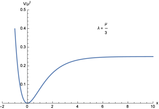
Figure 1: $V/\mu^{2}$ vs $x$.

One can now compute the spectral index $n_{s}$ and for tensor-to-scalar ratio $r$ in terms of the slow-roll inflation parameters $\epsilon$ and $\eta$. They are given by Ellis:2013xoa

$$\epsilon = \frac{1}{3}\mbox{csch}^{2}\frac{x}{\sqrt{6}}\,e^{-\sqrt{2/3}x}\,,$$ (5.15)

$$\eta = \frac{1}{3}\mbox{csch}^{2}\frac{x}{\sqrt{6}}\left(2e^{-\sqrt{2/3}x}-1\right)\,,$$ (5.16)

and the parameters $\{n_{s},r\}$ assume the values (in Planck units)

$$n_{s}=0.965\,,\quad r=0.0035\,,\quad x=5.35\,,\qquad\mbox{for}\quad N=55\,.$$

Let us now see how this inflationary model can be related to the Starobinsky model. We have already discussed the Starobinsky model as an example of extended theories of gravity (see Section 4). Here is interesting to show how the free parameter $M$ of the original Starobinsky model (i.e. $R+R^{2}/M^{2}$) can be related to the fundamental parameters coming from SUGRA. To this end, consider the conformal transformation

$$g_{\mu\nu}\quad\to\quad{\tilde{g}}_{\mu\nu}=\left(1+\frac{\varphi}{3M^{2}}\right)g_{\mu\nu}$$

and the redefinition of the field $\varphi$

$$\varphi\quad\to\quad\varphi^{\prime}=\sqrt{\frac{3}{2}}\,\ln\left(1+\frac{\varphi}{3M^{2}}\right)\,.$$

The Starobinsky action

$$S=\frac{1}{2}\int d^{4}x\sqrt{-g}\left(R+\frac{1}{6M^{2}}\,R^{2}\right)$$ (5.17)

assumes the form

$$S=\frac{1}{2}\int d^{4}x\sqrt{-{\tilde{g}}}\left[{\tilde{R}}+(\partial_{\mu}\varphi^{\prime})^{2}-V(\varphi^{\prime})\right]\,,$$ (5.18)

where the potential $V(\varphi^{\prime})$ is given by

$$V(\varphi^{\prime})=\frac{3}{4}M^{2}\left(1-e^{-\sqrt{2/3}\varphi^{\prime}}\right)^{2}\,.$$ (5.19)

The form of this potential is identical to the potential (5.14) obtained along the real direction of the no-scale Wess-Zumino model. Moreover, one can identify $M^{2}$ with $\mu$ according to the relation

$$M^{2}=\frac{\mu^{2}}{3}={\hat{\mu}}^{2}\,,$$

where the last equality follows for $c=\langle(T+T^{*})\rangle=1$. Thus, the Starobinsky parameter $M$ turns out to be directly related to the no-scale Wess-Zumino parameter ${\hat{\mu}}$ in the superpotential (4.45).

The Starobinsky model predicts that the tensor-to-scalar ratio is $r\simeq 10^{-3}$, which is in agreement with present experiment (BICEP2 reported a large value of the tensor-to-scalar ratio, $r=0.2^{+0.07}_{-0.05}$ BICEP2 , whereas the recent joint analysis by Planck + BICEP2 + Keck Array give the upper bound $r_{0.05}<0.12(95\%CL)$ BKP:2015 ; Ade:2015lrj ; Planck:2015 ).

5.2 The model $\xi\phi^{a}R^{b}$

We start with a general Higgs inflationary scenario $\xi\phi^{a}R^{b}$ in the framework of $f(\phi,R)$ gravity theory, which is a generalization of the Higgs inflation model $\xi\phi^{2}R$ Chakravarty:2013eqa . In the light of discoveries by CMS cms and ATLAS Atlas it is of interest to consider the Standard Model Higgs boson as the candidate for inflaton. However in the standard single-field slow-roll inflation with inflaton quartic potential, the idea of considering standard model Higgs as inflaton does not work as the inflaton quartic coupling should be of the order $\lambda\sim 10^{-12}$ to explain the amplitude of CMB perturbations measured by WMAP/Planck WMAP9 ; Planck:2015 while the 125 GeV Higgs has a quartic coupling $\lambda\sim 0.13$ at the electroweak scale which can however go down to smaller values at the Planck scale due to renormalization Sher . However just from the standard model renormalization one cannot have the Higgs coupling $\lambda\sim 10^{-12}$ over the entire range of the rolling field $\sim(10-1)M_{P}$ during inflation and the standard slow-roll inflation with a Higgs field does not give the observed amplitude and spectrum of density perturbations Isidori:2007vm . A way out of fine tuning the scalar self coupling to unnaturally small values was found out and it was shown that if one couples the scalar field to the Ricci scalar $\xi\phi^{2}R$ then the effective potential in the Einstein frame becomes a slow roll one with the effective scalar coupling being $\lambda/\xi^{2}$ and the amplitude of the density perturbations constrain this ratio Spokoiny:1984bd . Therefore for large $\xi$ small self-coupling $\lambda$ can be obtained as required. The equivalence of the density perturbation in Jordan and Einstein frame and density perturbations from inflation in the curvature coupled theories $\xi\phi^{2}R$ are studied in Kaiser:1994vs ; Komatsu:1997hv ; Komatsu:1999mt . Bezrukov and Shaposhnikov Bezrukov revived the large curvature coupling model to motivate the idea that the standard model Higgs field could serve as the inflaton in the early universe Bezrukov ; Barvinsky:2008ia . However the large value of non minimal coupling which fix the amplitude poses problem of unitarity violation at Planck scale Hertzberg:2010dc . Various ways to solve the unitarity violation have been explored in Barvinsky:2008ia ; giudice .

Here we assume that the dominant interaction between Higgs field and gravity is through operators of the form

$${\cal L}=\frac{\xi({\cal H}^{\dagger}{\cal H})^{a/2}R^{b}}{M_{p}^{a+2b-4}}.$$ (5.20)

This form (5.20) of Higgs Curvature interaction has been mentioned in Atkins:2010yg . The complete dynamics of the Higgs field involves the role of the Goldstone modes as has been studied in detail in Mooij:2011fi ; Kaiser:2010yu ; Greenwood:2012aj . The multifield dynamics of the Goldstone modes gives rise to sizable non-gaussianity. We will study the dynamics of the Higgs mode and impose a charge conservation and CP symmetry such that the Goldstone modes of the Higgs field do not acquire vevs. We will take the background Higgs field to be

$${\cal H}=\begin{pmatrix}0\\ \phi\end{pmatrix}$$ (5.21)

where $\phi$ is the Higgs mode with mass 126 GeV. This inflation model falls in the class of inflation in $f(\phi,R)$ theories studied in Ref. DeFelice:2010aj . The motivation is that we use the Higgs quartic coupling $\lambda({\cal H}^{\dagger}{\cal H})^{2}$ where the standard model value of $\lambda(\mu\sim M_{P})$ can lie in the range $\lambda=(10^{-5}-0.1)$ depending on the value of top quark mass Sher or on new physics Chakrabortty:2012np . We take curvature coupling $\xi$ to be unity and check the possibility of generating the observed density perturbations from Higgs inflation by varying parameters $a$, $b$ and $\lambda$. The non minimal coupling $\xi$ has been taken unity in order to improve the unitarity behavior which increases the natural cutoff scale $\Lambda$ from $\Lambda\simeq\frac{M_{p}}{\xi}\simeq 10^{15}$ to $\Lambda\simeq M_{p}\simeq 10^{19}$.

In non-minimal $\xi\phi^{2}R$ theory we can always make a conformal transformation to the Einstein frame so one can compute the density perturbations either in Einstein frame or Jordan frame and the gauge invariant curvature perturbations should be same in both the frames Kaiser:1994vs . With the $\xi\phi^{a}R^{b}$ model we find that no conformal transformation exists which can in general remove this term to go to an Einstein frame. We find that in $\xi\phi^{a}R^{b}$ theory such a conformal transformation is only possible if the metric is quasi-de Sitter. The accurate comparison with the experimental data should be made however with the Jordan frame results. The curvature perturbation in both Einstein and Jordan frame for the $\xi\phi^{2}R$ theory has been derived in Kaiser:1994vs ; Gong:2011qe ; prokopec .

5.2.1 Model in the Jordan Frame

Consider the action for a scalar field interacting with gravity of the form

$$S_{J}=\int d^{4}x\sqrt{-g}\left[-\frac{f(\phi,R)}{2\kappa^{2}}+\frac{1}{2}g^{\mu\nu}\partial_{\mu}\phi\partial_{\nu}\phi+V(\phi)\right]\ ,$$ (5.22)

where

$$\frac{1}{\kappa^{2}}f(\phi,R) = \frac{1}{\kappa^{2}}R+\frac{\xi\phi^{a}R^{b}}{M_{p}^{a+2b-4}}$$ (5.23)

$$V(\phi) = \frac{\lambda\phi^{4}}{4}\,,$$ (5.24)

and $\xi$ is a dimensionless coupling constant. Setting

$$F\equiv\frac{\partial{f}}{\partial{R}}=1+\frac{\xi b\phi^{a}R^{b-1}}{M_{p}^{a+2b-2}}$$

the field equations read

$$FR_{\mu\nu} - \frac{1}{2}fg_{\mu\nu}-\triangledown_{\mu}\triangledown_{\nu}F+g_{\mu\nu}\square F=\kappa^{2}\left(\triangledown_{\mu}\phi\triangledown_{\nu}\phi-\frac{1}{2}g_{\mu\nu}\triangledown^{\rho}\phi\triangledown_{\rho}\phi-Vg_{\mu\nu}\right),$$ (5.25)

$$\square{\phi} = V_{,\phi}-\frac{f_{,\phi}}{2\kappa^{2}},$$ (5.26)

For the unperturbed background FRW metric (1.4) the above Eqs. (5.25) and (5.26) give

$$3FH^{2}+\frac{1}{2}\left(f-RF\right)+3H\dot{F} = \kappa^{2}\left(\frac{1}{2}\dot{\phi}^{2}+V(\phi)\right)\,,$$ (5.27)

$$-2F\dot{H}-\ddot{F}+H\dot{F} = \kappa^{2}\dot{\phi}^{2}\,,$$ (5.28)

$$\ddot{\phi}+3H\dot{\phi}+V_{,\phi}-\frac{f_{,\phi}}{2\kappa^{2}} = 0\,.$$ (5.29)

We assume that the second term of $F$ $i.e.$ $\frac{\xi b\phi^{a}R^{b-1}}{M_{p}^{a+2b-2}}$ is dominant for some values of $a$ and $b$. We find this assumption to be valid while solving numerically for the values of $a$ and $b$ in our model which give rise to the experimentally observed density perturbations. From Eq. (5.27), under this assumption and considering the slow-roll parameters as small (see below their definition, Eq. (5.38)), the Hubble parameter in the Jordan frame reads

$$H=\frac{\lambda^{\frac{1}{2b}}}{\sqrt{12}\big{[}\xi(2-b)\big{]}^{\frac{1}{2b}}}\left(\frac{\phi}{M_{p}}\right)^{\frac{4-a}{2b}}M_{p}\ .$$ (5.30)

From equation (5.29) under the slow-roll assumption we get

$$\dot{\phi}=-\frac{\lambda\phi^{3}}{3H}\Big{[}1-\frac{a}{2(2-b)}\Big{]}.$$ (5.31)

Now we perturb Eqs. (5.25) and (5.26) by perturbing the scalar field $\phi=\phi(t)+\delta\phi(x,t)$ and the metric (3.42) DeFelice:2010aj . One can derive the Einstein field equations for the $f(R,\phi)$ theory keeping the linear terms in the metric and scalar field perturbations hwang ; hwang1 and the equation of motion of scalar perturbation. The relevant quantity is the curvature perturbation

$$\mathcal{R}=\Psi-H\delta\phi/\dot{\phi}\,,$$

where we work in the gauge $\delta\phi=0$ and $\delta R=0$. This sets $\mathcal{R}=\Psi$ (notice that $\delta F=0$ since $\delta F=\left(\partial F/\partial\phi\right)\delta\phi+\left(\partial F/\partial R\right)\delta R$). Owing to this gauge the equation for $\Phi$ reads

$$\Phi=\frac{\dot{\mathcal{R}}}{H+\dot{F}/(2F)}$$ (5.32)

while the equation for $\Phi$, $\Psi$, $E$ and $B$, is given in terms of the combination

$$A\equiv 3(H\Phi-{\dot{\Psi}})-\frac{\Delta{\tilde{B}}}{a^{2}}=-\frac{1}{H+\dot{F}/(2F)}\left(\frac{\triangle}{a^{2}(t)}\mathcal{R}+\frac{\left(3H\dot{F}-\kappa^{2}\dot{\phi}^{2}\right)\mathcal{\dot{R}}}{2F\left(H+\dot{F}/(2F)\right)}\right)\,.$$ (5.33)

where

$${\tilde{B}}\equiv a(t)(E+a(t){\dot{B}})\,.$$

The differential equation for curvature perturbation is

$$\ddot{\mathcal{R}}+\frac{(a^{3}(t)Q_{s})\dot{}}{a^{3}(t)Q_{s}}\dot{\mathcal{R}}+\frac{k^{2}}{a^{2}(t)}\mathcal{R}=0,$$ (5.34)

where

$$Q_{s}\equiv\frac{\dot{\phi}^{2}+3\dot{F}^{2}/(2\kappa^{2}F)}{\left(H+\dot{F}/(2F)\right)^{2}}\,.$$

Introducing the variables

$$\omega=a(t)\sqrt{Q_{s}},\quad\sigma_{k}=\omega\mathcal{R}\,,$$

one may re-write the equation (5.34) as

$$\sigma_{k}^{\prime\prime}+\left(k^{2}-\frac{\omega^{\prime\prime}}{\omega}\right)\sigma_{k}=0,$$ (5.35)

where prime denotes the derivative with respect to the conformal time defined as $d\eta=dt/a(t)$ and

$$\frac{\omega^{\prime\prime}}{\omega} = \frac{a^{\prime\prime}(t)}{a(t)}+\frac{a^{\prime}(t)}{a(t)}\frac{Q_{s}^{\prime}}{Q_{s}}+\frac{1}{2}\frac{Q_{s}^{\prime\prime}}{Q_{s}}-\frac{1}{4}\left(\frac{Q_{s}^{\prime}}{Q_{s}}\right)^{2}$$

$$= \frac{1}{\eta^{2}}\Big{[}\nu_{\mathcal{R}}^{2}-\frac{1}{4}\Big{]}\,,$$

where the last term follows from under quasi de-Sitter expansion $a(\eta)=\frac{-1}{H\eta(1-\epsilon_{1})}$, so that

$$\frac{a^{\prime\prime}(t)}{a(t)}=\frac{1}{\eta^{2}}\big{[}2+3\epsilon_{1}\big{]}\,,\quad\frac{a^{\prime}(t)}{a(t)}=a(t)H\,,$$

and

$$\nu_{\mathcal{R}}^{2}=\frac{9}{4}\Big{[}1+\frac{4}{3}\left(2\epsilon_{1}+\epsilon_{2}-\epsilon_{3}+\epsilon_{4}\right)\Big{]}.$$ (5.37)

$$\epsilon_{1}=-\frac{\dot{H}}{H^{2}}\ ,\ \epsilon_{2}=\frac{\ddot{\phi}}{H\dot{\phi}}\ ,\ \epsilon_{3}=\frac{\dot{F}}{2HF}\ ,\ \epsilon_{4}=\frac{\dot{E}}{2HE}\ ;$$ (5.38)

$$E=F+\frac{3\dot{F}^{2}}{2\kappa^{2}\dot{\phi}^{2}}=\frac{Q_{s}(1+\epsilon_{3})^{2}}{\dot{\phi}^{2}/(FH^{2})}\ .$$ (5.39)

Here $\epsilon_{i}$ are slow-roll parameters and $\dot{\epsilon_{i}}$ terms have been neglected. Equation (5.35) then has solutions in the Hankel functions of order $\nu_{R}$

$$\sigma=\frac{\sqrt{\pi|\eta|}}{2}e^{i(1+2\nu_{\mathcal{R}})\pi/4}\left[c_{1}\,H_{\nu_{\mathcal{R}}}^{(1)}(k|\eta|)+c_{2}\,H_{\nu_{\mathcal{R}}}^{(2)}(k|\eta|)\right]$$ (5.40)

Applying the Bunch-Davies boundary condition

$$\sigma(k\eta\rightarrow-\infty)=e^{ik\eta}/\sqrt{2k}\,,$$

we fix the integration constants $c_{1}=1$ and $c_{2}=0$. Using the relation

$$H_{\nu}(k|\eta|)=\frac{-i}{\pi}\Gamma(\nu)\left(\frac{k|\eta|}{2}\right)^{-\nu}\,,$$

for the super-horizon modes $k\eta\rightarrow 0$, we obtain the expression for the power spectrum of curvature perturbations which is defined as (3.103)

$${\mathcal{P}}_{\mathcal{R}} = \frac{k^{3}}{2\pi^{2}}\langle|\mathcal{R}|^{2}\rangle$$

$$\equiv {\Delta}_{\mathcal{R}}^{2}\left(\frac{k}{a(t)H}\right)^{n_{\mathcal{R}}-1},$$

where the amplitude of the curvature power spectrum turns out to be

$${\Delta}^{2}_{\mathcal{R}}=\frac{1}{Q_{s}}\left(\frac{H^{2}}{4\pi^{2}}\right)$$ (5.42)

and the spectral index is

$$n_{\mathcal{R}}-1 = 3-2\nu_{\mathcal{R}}$$

$$\simeq -4\epsilon_{1}-2\epsilon_{2}+2\epsilon_{3}-2\epsilon_{4}$$

$$\simeq -6\epsilon_{1}\,.$$

In this $f(\phi,R)$ model one gets

$$\epsilon_{1}\approx-\epsilon_{3}\,,\quad\epsilon_{2}\approx-\epsilon_{4}\,,$$

where

$$\epsilon_{1} = b^{-1}(a-4)(2-b)^{(1-b)/b}(a+2b-4)\lambda^{(b-1)/b}\xi^{1/b}\left(\frac{\phi}{M_{p}}\right)^{\frac{a+2b-4}{b}}$$ (5.44)

$$\epsilon_{2} = b^{-1}(a+6b-4)\left(2-b\right)^{(1-b)/b}(a+2b-4)\lambda^{(b-1)/b}\xi^{1/b}\left(\frac{\phi}{M_{p}}\right)^{\frac{a+2b-4}{b}}.$$ (5.45)

The expressions for the amplitude of power spectrum and the number of e-folding are

$$\Delta_{\mathcal{R}}^{2}=\frac{b[(2-b)/\lambda]^{3-\frac{4}{b}}M_{p}^{8+\frac{4(a-4)}{b}}\xi^{-\frac{4}{b}}\phi^{-\frac{4(a+2b-4)}{b}}}{288(a-4)^{2}(a+2b-4)^{2}\pi^{2}}$$ (5.46)

and

$$N_{J}=\int_{\phi_{J}}^{\phi_{f}}\frac{H}{\dot{\phi}}d\phi=\frac{b[(2-b)/\lambda]^{\frac{b-1}{b}}\xi^{-\frac{1}{b}}}{2(a+2b-4)^{2}}\left(\frac{\phi}{M_{p}}\right)^{\frac{4-a-2b}{b}}\Bigg{|}^{\phi_{J}}_{\phi_{f}}$$ (5.47)

respectively. Here $\phi_{J}$ and $\phi_{f}$ are the values of scalar field $\phi$ at the beginning and the end of inflation respectively.

Let us compute the tensor perturbation of the field equations (5.25). Setting $D_{ij}=h_{ij}/a^{2}$ and using the polarization tensors $e_{ij}^{1}$ and $e_{ij}^{2}$, such that the tensor $D_{ij}$ can be written as

$$D_{ij}=D_{1}e_{ij}^{1}+D_{2}e_{ij}^{2}\,,$$

the equation for the tensor perturbation reads

$$\ddot{D}_{\lambda}+\Xi\,\dot{D}_{\lambda}+\frac{\kappa^{2}}{a^{2}}D_{\lambda}=0,$$ (5.49)

where $\lambda\equiv 1,2$ corresponds to two polarizations of gravity wave, and

$$\Xi=\frac{1}{a^{3}F}\frac{d}{dt}\,a^{3}F\,.$$

Substituting

$$z=a\sqrt{F}\,,\qquad v_{k}=\frac{1}{\sqrt{2}}\,zD_{\lambda}M_{P}\,,$$

we get

$$v_{\lambda}^{\prime\prime}+\left(k^{2}-\frac{z^{\prime\prime}}{z}\right)v_{\lambda}=0,$$ (5.50)

where ^′ stands for the derivative with respect to conformal time. To obtain the amplitude of power spectrum of $D_{\lambda}$, one has to sum over all polarization states. Equation (5.50) yields

$$\Delta^{2}_{T} = 4\times\left(\frac{2}{M_{p}^{2}}\right)\frac{k^{3}}{2\pi^{2}}\frac{1}{a^{2}F}v_{\lambda}^{2}$$

$$\simeq \frac{2}{\pi^{2}}\left(\frac{H}{M_{P}}\right)^{2}\frac{1}{F}\,.$$

The ratio of the amplitude of tensor perturbations to scalar perturbations $r$ is given by

$$r\equiv\frac{\Delta^{2}_{T}}{\Delta^{2}_{\mathcal{R}}}=\frac{8Q_{s}}{M_{p}^{2}F}\simeq 48\epsilon_{3}^{2}\,.$$ (5.52)

5.2.2 Model in the Einstein Frame

Our aim is to compute the action (5.22), with $V=\lambda\phi^{4}/4$, in the JF

$$S_{J}=\int d^{4}x\sqrt{-g}\left[-\frac{{M_{p}}^{2}}{2}R\left(1+\frac{\xi\phi^{a}R^{b-1}}{M_{p}^{a+2b-2}}\right)+\frac{1}{2}\partial_{\mu}\phi\partial^{\mu}\phi+\frac{\lambda\phi^{4}}{4}\right]$$ (5.53)

We use the a conformal transformation of the metric and Ricci scalar, see Eqs. (4.1), with the conformal factor given by

$$\Omega^{2}=1+\frac{\xi\phi^{a}R^{b-1}}{{M_{p}}^{a+2b-2}}\ .$$ (5.54)

For quasi de-Sitter space we may ignore the second and third terms in the bracket in Eq. (4.1) (we have $\{{\dot{\Omega}}/\Omega,{\ddot{\Omega}}/\Omega\}\ll 1$, as will be showed in (5.68)). We therefore write (5.54) in EF as

$$\Omega^{2}=1+\frac{\xi^{1+q}\phi^{p}{\tilde{R}}^{q}}{M_{p}^{p+2q}}\,,$$ (5.55)

where

$$p=\frac{a}{2-b}\,,~{}~{}~{}~{}~{}~{}~{}q=\frac{b-1}{2-b}\,,~{}~{}~{}~{}~{}~{}\tilde{R}=12\tilde{H}^{2}\simeq Constant\,.$$ (5.56)

Via conformal transformation we write the action (5.53) in term of new field $\chi$

$$S_{E}=\int d^{4}x\left(-\frac{M_{p}^{2}}{2}\tilde{R}+\frac{1}{2}\partial^{\mu}{\chi}\partial_{\mu}\chi+U(\chi)\right),$$ (5.57)

where

$$\frac{d\chi}{d\phi} = \frac{1}{\Omega^{2}}\left(\Omega^{2}+\frac{3p^{2}\xi^{\prime 2}}{2}\left(\frac{\phi}{M_{p}}\right)^{2p-2}\right)^{1/2}\,,~{}~{}~{}~{}~{}~{}~{}\xi^{\prime}\equiv\xi^{1+q}\left(\frac{12\tilde{H}^{2}}{M_{p}^{2}}\right)^{q}$$

$$U(\chi) = \frac{1}{\Omega^{4}}\frac{\lambda}{4}\phi(\chi)^{4}.$$ (5.58)

For $\phi\gg M_{P}/\xi^{\prime 1/p}$, Eq. (5.2.2) can be integrated to give

$$\phi(\chi)=\frac{M_{p}}{\xi^{\prime\,1/p}}\exp\left(\sqrt{\frac{2}{3}}\frac{\chi}{M_{p}p}-\frac{1}{2}\right).$$ (5.59)

Considering

$$\tilde{g}_{\mu\nu}=diag(-M^{2}(t),\tilde{a}^{2}(t),\tilde{a}^{2}(t),\tilde{a}^{2}(t))$$

and varying the action (5.57) with respect to $M(t)$ or $a(t)$ and setting $M=1$ in the final equation which corresponds FRW metric, we get the Friedmann equation

$$12\tilde{H}^{2}-\zeta^{-1}M_{p}^{2}\lambda\left(1+\frac{2q}{p}\right)=0\ ,$$ (5.60)

where

$$\zeta=12^{4q/p}\left(\frac{\tilde{H}^{2}}{M_{p}^{2}}\right)^{4q/p}\xi^{\frac{4(1+q)}{p}}\exp\left(2\sqrt{\frac{2}{3}}\frac{(p-2)\chi}{pM_{p}}\right).$$ (5.61)

All the derivative terms of Hubble parameter $\tilde{H}$ have been neglected (this is corresponds to slow roll condition, $i.e.$, $\dot{\chi}^{2}$ is much smaller than potential term). From (5.60) the Hubble parameter assumes the form

$$\tilde{H}=M_{p}\frac{\left[\left(1+2q/p\right)\lambda\right]^{\frac{p}{2(p+4q)}}}{\sqrt{12}\ \xi^{\frac{2(1+q)}{p+4q}}}\exp\Bigg{[}\sqrt{\frac{2}{3}}\left(\frac{2-p}{p+4q}\right)\frac{\chi}{M_{p}}\Bigg{]}\ .$$ (5.62)

Using Eqs. (5.55) and (5.62) into (5.58) one infers the scalar potential

$$U(\chi)=\frac{1}{4}M_{p}^{4}\lambda^{\frac{p}{p+4q}}\xi^{-\frac{4(1+q)}{p+4q}}\left(1+\frac{2q}{p}\right)^{-\frac{4q}{p+4q}}\exp\Big{[}2\sqrt{\frac{2}{3}}\left(\frac{2-p}{p+4q}\right)\frac{\chi}{M_{p}}\Big{]}.$$ (5.63)

In deriving (5.63) the large field approximation $\exp(\sqrt{\frac{2}{3}}\frac{\chi}{M_{p}})\gg 1$ for $\chi\gg M_{p}$ has been used. Also the parameters $a$ and $b$, which appear through $p$ and $q$ as defined above, in the potential (5.63) are the parameters of the JF action (5.53) which appear in the EF potential via conformal transformation of the metric (4.1). The spectral index and curvature perturbation can be computed by using above potential (5.63). The slow-roll parameters for large $\chi\gg M_{p}$ comes out to be

$$\epsilon = \frac{M_{p}^{2}}{2}\left(\frac{U^{\prime}}{U}\right)^{2}=\frac{4}{3}\left(\frac{a+2b-4}{a+4b-4}\right)^{2}\,,$$ (5.64)

$$\eta = M_{p}^{2}\left(\frac{U^{\prime\prime}}{U}\right)=\frac{8}{3}\left(\frac{a+2b-4}{a+4b-4}\right)^{2}\,,$$

and the amplitude of curvature perturbations (3.4)

$$\Delta^{2}_{\mathcal{R}} = \frac{1}{8\pi^{2}\epsilon}\frac{\tilde{H}^{2}}{M_{p}^{2}}$$

$$= \frac{1}{128\pi^{2}}\left(\frac{y+2}{2y-x+4}\right)^{\frac{x+2y+4}{x}}\lambda^{\frac{2y-x+4}{x}}\xi^{-\frac{4}{x}}\left(\frac{x}{y}\right)^{2}e^{-2\sqrt{\frac{2}{3}}\frac{y}{x}\frac{\chi}{M_{p}}}\,,$$

where

$$x=a+4b-4,\qquad y=a+2b-4\,.$$

The spectral index in the term of slow-roll parameters is (3.4)

$$n_{s}=1-6\epsilon+2\eta.$$ (5.66)

The number of e-folding is calculated as

$$N_{E}=\int^{{\chi}_{0}}_{{\chi}_{e}}\frac{U(\chi)}{U^{\prime}(\chi)}d\chi=-\frac{1}{2}\sqrt{\frac{3}{2}}\left(\frac{x}{y}\right)\left(\frac{{\chi}_{0}-{\chi}_{e}}{M_{p}}\right)$$ (5.67)

For ${\chi}_{0}\sim 13M_{p}$ and ${\chi}_{e}\sim 1M_{p}$, the number of e-folding is found to be around $60$. From equation (5.54) and (5.59), one can calculate the order of terms like $\ddot{\Omega}/\Omega$ and $(\dot{\Omega}/\Omega)^{2}$ for $\phi\gg\frac{M_{p}}{\xi^{1/p}}$. For $\lambda=10^{-3}$ and $\xi=1$, one gets

$$\frac{\ddot{\Omega}}{\Omega} \sim \frac{U}{9M_{p}^{2}}(\epsilon+\sqrt{3\epsilon}(\eta-\epsilon))=4.1\times 10^{-11}M_{p}^{2}\,,$$ (5.68)

$$\left(\frac{\dot{\Omega}}{\Omega}\right)^{2} \sim \frac{U}{9M_{p}^{2}}\epsilon=3.3\times 10^{-11}M_{p}^{2}\,,$$

whereas the value of curvature scalar $\tilde{R}=12\tilde{H}^{2}$ at the same values of parameter is $4.1\times 10^{-8}M_{p}^{2}$. Thus the approximation we have made is consistent. We now use the measured values of these CMB anisotropy parameters to get the numerical values for the parameters $(a,b,\xi,\lambda)$.

Results and Discussion

Planck$+$WP measurements Planckgroup provides that the curvature perturbation is $\Delta_{\mathcal{R}}^{2}=2.195^{+0.533}_{-0.585}\times 10^{-9}$, spectral index is $n_{\mathcal{R}}=0.9603\pm 0.0073$ and the tensor to scalar ratio $r<0.11(95\%CL)$ (see (2.32)-(2.38)). Equation (5.67) implies that to get $60$ e-foldings, the scalar field $\chi$ should roll from $13M_{p}$ to $1M_{p}$. In Table 1 are reported the values of parameters $\{\lambda,a,b\}$ giving the measured values of $\Delta_{\mathcal{R}}^{2}$ and $n_{s}$. Here $\xi=1$ and $\lambda$ $\xi=1$ assumes different values.

The slow-roll parameters are $\epsilon\sim 0.02$ and $\eta\sim 0.04$. In particular, for $\epsilon\simeq 0.02$ the tensor-to-scalar ratio in EF is predicted to be large $r\simeq 0.3$.

Table 1: The values of parameters $a$ and $b$ in the Einstein frame at $\chi_{0}=13M_{p}$ with $\xi=1$ for different values of $\lambda$. The parameters $a$ and $b$ of the Jordan frame action appears in the Einstein frame potential via conformal transformation of the metric.

$\ \lambda$	$\ 0.1$	$\ 10^{-2}$	$\ 10^{-3}$	$\ 10^{-4}$	$\ 10^{-5}$
a	$\ 3.385$	$\ 3.026$	$\ 2.735$	$\ 2.494$	$\ 2.292$
b	$\ 0.277$	$\ 0.439$	$\ 0.571$	$\ 0.679$	$\ 0.770$
a+2b	$\ 3.939$	$\ 3.904$	$\ 3.877$	$\ 3.852$	$\ 3.832$

We evaluate now the observables in JF using (5.46) and (5.2.1) for $\xi=1$. In Table 2 are displayed the values of the scalar field $\phi$ in the JF corresponding to $\chi_{e}=1M_{p}$ and $\chi_{0}=13M_{p}$ for different values of $\lambda$. Using these values of the range of the roll in $\phi$ we see that the number of e-foldings $N_{J}$ in the JF, corresponding to $N_{E}=60$ is $N_{J}\sim 830$. The values of $\{\lambda,a,b\}$, required to get the curvature perturbation and spectral index, are shown in the Table 2. The slow-roll parameters are found to be $\epsilon_{1}\simeq-\epsilon_{3}\simeq 0.007$ and $\epsilon_{2}\simeq-\epsilon_{4}\simeq-0.013$ for chosen range of $\lambda$. For these values, the tensor-to-scalar ratio is small $r\simeq 0.002$ in JF. Two comments are in order: 1) The assumptions $F=1+\frac{\xi b\phi^{a}R^{b-1}}{M_{p}^{a+2b-2}}\gg 1$ and $\frac{\kappa^{2}\dot{\phi}^{2}}{FH^{2}}\ll 6\epsilon_{3}^{2}$ are verified for the best fit values of the above parameters. 2) In the limit $a\simeq 2$ and $b\simeq 1$, the correct value of $\Delta_{\mathcal{R}}^{2}$ and $n_{\mathcal{R}}$ are obtained for $\lambda\sim 0.1$ only for large value of $\xi\sim 10^{4}$, in agreement with the prediction of Higgs inflation models $\xi\phi^{2}R$  Bezrukov ; Bezrukov1 .

Table 2: The values of parameters $a$ and $b$ are evaluated in the Jordan frame at $\xi=1$ and $\phi_{J}|_{{}_{\chi_{0}=13M_{p}}}$ for different values of $\lambda$.

$\ \lambda$	$\ 0.1$	$\ 10^{-2}$	$\ 10^{-3}$	$\ 10^{-4}$	$\ 10^{-5}$
$\phi_{f}|_{{}_{(\chi_{e}=1M_{p})}}$	$\ 0.0146M_{p}$	$\ 0.0253M_{p}$	$\ 0.044M_{p}$	$\ 0.077M_{p}$	$\ 0.134M_{p}$
$\phi_{J}|_{{}_{(\chi_{0}=13M_{p})}}$	$\ 3.566M_{p}$	$\ 6.187M_{p}$	$\ 10.77M_{p}$	$\ 18.8M_{p}$	$\ 32.77M_{p}$
a	$\ 3.56398962$	$\ 3.2751299$	$\ 3.0257694$	$\ 2.809561$	$\ 2.620851$
b	$\ 0.21800513$	$\ 0.3624348$	$\ 0.4871146$	$\ 0.595217$	$\ 0.689566$
a+2b	$\ 3.999999$	$\ 3.999999$	$\ 3.999998$	$\ 3.999995$	$\ 3.99998$

To summarize, this model ${\xi\phi^{a}R^{b}}$ is a generalization of the Higgs inflation model ${\xi\phi^{2}R}$ with $\lambda\phi^{4}$ potential. We find that if the Higgs self coupling $\lambda$ is in the range $(10^{-5}-0.1)$, parameter $a$ in the range $(2.3-3.6)$ and $b$ in the range $(0.77-0.22)$ at the Planck scale, one can have a viable inflation model even for $\xi\simeq 1$. $\lambda\sim 0.1$ in this model solve the fine tuning problem of Higgs self-coupling in the standard slow-roll inflation which predict $\lambda\sim 10^{-12}$. The tensor-to-scalar ratio $r$ in this model in EF is large $r\simeq 0.3$, therefore model with generalized scalar-curvature couplings is ruled out by observational limits on $r$ like the pure $\frac{\lambda}{4}\phi^{4}$ theory. However, with independent calculations in JF gives small $r\simeq 0.002$ which is allowed from the observations. Therefore, JF result contradicts the EF result. The observations should be compared with EF results or JF results is still matter of debate. However in this model, by requiring the curvature coupling parameter to be of order unity, we have evaded the problem of unitarity violation in scalar-graviton scatterings which plague the $\xi\phi^{2}R$ Higgs inflation models. Therefore, the Higgs field may still be a good candidate for being the inflaton in the early universe if one considers higher dimensional curvature coupling. Also we find that, upto slow-roll approximation, for the same set of parameter values ($\xi,\lambda$) the set of ($a$,$b$) values is nearly the same in Jordan and Einstein frames. Therefore, the Einstein and Jordan frames are equivalent. In this model, we found a symmetry $a+2b\approx 4$ which holds true in both the frame and it implies that the curvature coupling $\xi$ is nearly scale invariant.

5.3 The power law model $R+R^{\beta}$

We now study a model $R+\frac{1}{M^{2}}R^{\beta}$ of inflation which is a generalization of Starobinsky model $R+\frac{1}{M^{2}}R^{2}$ and so we call it as power law Starobinsky model Chakravarty:2014yda . $M$ and $\beta$ are the two dimensionless parameters. In general scalar-curvature theories the scalar plays the role of the inflaton after transforming to Einstein frame whereas in pure curvature theories like $R+\frac{1}{M^{2}}R^{\beta}$ model the longitudinal part of the graviton is the equivalent scalar in the Einstein frame plays the role of inflaton. Along with the independent observable predictions of this model, we will show that generalized Higgs inflation model $\xi\phi^{a}R^{b}$ is equivalent to power law Starobinsky model.

The Starobinsky model of inflation starobinsky2 with an $\frac{1}{M^{2}}R^{2}$ interaction term is of interest as it requires no extra scalar fields but relies on the scalar degree of the metric tensor to generate the ’inflaton’ potential. The $R^{2}$ correction to Einstein gravity is, as we have before seen, equivalent to scalar-tensor theory with a scalar potential which is an exponentially corrected plateau potential Bezrukov . This model is favored by the Planck constraint on the tensor to scalar ratio which ruled out potentials like $m^{2}\phi^{2}$ and $\lambda\phi^{4}$ in the context of standard slow-roll inflation. The characteristic feature of the Starobinsky equivalent models was the prediction that the tensor-to-scalar ratio was $r\simeq 10^{-3}$. BICEP2 reported a large value of $r=0.2^{+0.07}_{-0.05}$ BICEP2 but the recent joint analysis by Planck + BICEP2 + Keck Array give only an upper bound of $r_{0.05}<0.07(95\%CL)$ BKP:2015 ; Ade:2015xua . In an analysis of the genus structure of the B-mode polarisation of Planck + BICEP2 data by Colley et al. put the tensor-to-scalar ratio at $r=0.11\pm 0.04(68\%CL)$ Colley:2014nna . In the light of the possibility that $r$ can be larger than the Starobinsky model prediction of $r\sim 0.003$, generalisations of the Starobinsky model are of interest. The quantum correction on $\phi^{4}$-potential in Jordan frame was studied in Kehagias:2013mya ; Joergensen:2014rya ; Codello:2014sua ; Gao:2014fha where they have shown the equivalence of the $\xi\phi^{2}R+\lambda\phi^{4(1+\gamma)}$ model with $\frac{1}{M^{2}}R^{\beta}$ model. The generalized Starobinsky model with $R^{p}$ correction has been studied in the ref. stelle .

The action is given by DeFelice:2010aj ; Nojiri:2010wj

$$S_{J}=\int d^{4}x\sqrt{-g}f(R)\,,\qquad f(R)=-\frac{M_{p}^{2}}{2}\left(R+\frac{1}{6M^{2}}\frac{R^{\beta}}{M_{p}^{2\beta-2}}\right)$$ (5.69)

Consider the conformal transformation

$$\Omega=F=\frac{\partial f(R)}{\partial R}$$

and the new scalar field $\chi$ defined by

$$\Omega\equiv\exp\left(\frac{2\chi}{\sqrt{6}M_{p}}\right)\,.$$

The action (5.69) gets transformed in the EF (see Section 4) as

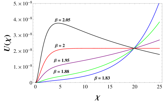
Figure 2: The nature of the potential (5.71) for different $\beta$ values (with $M=1.7\times 10^{-4}$). The potential and the field values are in $M_{p}=1$ units.

$$S_{E}=\int d^{4}x\sqrt{-\tilde{g}}\left[\frac{-M_{p}^{2}}{2}\tilde{R}+\frac{1}{2}\tilde{g}^{\mu\nu}\partial_{\mu}\chi\partial_{\nu}\chi+U(\chi)\right]\,,$$ (5.70)

where $U(\chi)$ is can be written in the EF as

$$U(\chi) = \frac{\left(RF(R)-f(R)\right)M_{p}^{2}}{2F(R)^{2}}$$ (5.71)

$$= \frac{(\beta-1)}{2}\left(\frac{6M^{2}}{\beta^{\beta}}\right)^{\frac{1}{\beta-1}}\exp\left[\frac{2\chi}{\sqrt{6}}\bigg{(}\frac{2-\beta}{\beta-1}\bigg{)}\right]\left[1-\exp\bigg{(}\frac{-2\chi}{\sqrt{6}}\bigg{)}\right]^{\frac{\beta}{\beta-1}}\,$$

with $f(R)$ given in (5.69) ($M_{p}=1$). Also we see that in the limit $\beta\rightarrow 2$ potential (5.71) reduces to exponentially corrected flat plateau potential of the Starobinsky model. Assuming large field limit $\chi\gg\frac{\sqrt{6}}{2}$ and $1<\beta<2$, the potential (5.71) reduces to

$$U(\chi)\simeq\frac{(\beta-1)}{2}\left(\frac{6M^{2}}{\beta^{\beta}}\right)^{\frac{1}{\beta-1}}\exp\Bigg{[}\frac{2\chi}{\sqrt{6}}\bigg{(}\frac{2-\beta}{\beta-1}\bigg{)}\Bigg{]}$$ (5.72)

We shall use Eq. (5.72) to compare with SUGRA version of the power law potential in the large field limit.

In Fig.2 it is plotted the potential for small deviations from the Starobinsky model value $\beta=2$. We see that the potential is very flattest for $\beta=2$ but becomes very steep even with small deviation from Starobinsky model value $\beta=2$. The scalar curvature perturbation $\Delta^{2}_{\mathcal{R}}\propto\frac{U(\chi)}{\epsilon}$ is fixed from observations which implies that the magnitude of the potential $U(\chi)$ would have to be larger as $\epsilon$ increases for steep potential to maintain the level of observed amplitude $\Delta^{2}_{\mathcal{R}}$. The tensor perturbation which depends on the magnitude of $U(\chi)$ therefore increases rapidly as $\beta$ varies from $2$. The variation of $r$ with $\beta$ is shown in the Fig. 4.

From Eq. (5.71), in the large field approximation, the slow-roll parameters in Einstein frame can be obtained as

$$\epsilon = \frac{1}{2}\left(\frac{U^{\prime}}{U}\right)^{2}\simeq\frac{1}{3}\left[\frac{\beta(3-2\beta)}{(\beta-1)^{2}}\exp\left(\frac{-2\chi}{\sqrt{6}}\right)+\frac{\beta-2}{\beta-1}\right]^{2},$$ (5.73)

$$\eta = \frac{U^{\prime\prime}}{U}\simeq\frac{-2}{3}\left[\frac{\beta(3-2\beta)^{2}}{(\beta-1)^{3}}\exp\left(\frac{-2\chi}{\sqrt{6}}\right)-\frac{(\beta-2)^{2}}{(\beta-1)^{2}}\right],$$ (5.74)

$$\xi = \frac{U^{\prime}U^{\prime\prime\prime}}{U^{2}}\simeq\frac{4\sqrt{\epsilon}}{3\sqrt{3}}\left[\frac{\beta(3-2\beta)^{3}}{(\beta-1)^{4}}\exp\left(\frac{-2\chi}{\sqrt{6}}\right)+\frac{(\beta-2)^{3}}{(\beta-1)^{3}}\right].$$ (5.75)

The field value $\chi_{e}$ at the end of inflation can be fixed from Eq. (5.73) by using the end of inflation condition $\epsilon\simeq 1$. And the initial scalar field value $\chi_{s}$ corresponding to $N=60$ e-folds before the end of inflation, when observable CMB modes leave the horizon, can be fixed by using the e-folding expression

$$N=\int_{\chi_{e}}^{\chi_{s}}\frac{U(\chi)}{U^{\prime}(\chi)}d\chi\,.$$

Under slow-roll approximation, one can use the standard Einstein frame relations for the amplitude of the curvature perturbation $\Delta_{\mathcal{R}}^{2}$, the spectral index $n_{s}$ and its running $\alpha_{s}$, and the tensor-to-scalar ratio $r$ to fix the parameters of the model.

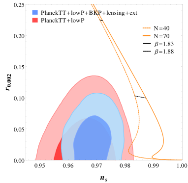
Figure 3: The regions of $(n_{s},r)$ allowed by Planck-2015 and joint BKP analysis at $68\%CL$ and $95\%CL$ are shown Ade:2015xua . The colored contour lines are the predictions for our model for two sets of $\beta$ and $N$ values corresponding to $M\approx 10^{-4}$ which satisfies the observed amplitude of the CMB power spectrum.

From CMB observations, for 7-parameter $\Lambda CDM$+$r$ model, when there is no scale dependence of the scalar and tensor spectral indices the bound on $r$ is $r_{0.002}<0.07$ ($95\%CL$, PlanckTT+lowP) and the amplitude, the spectral index and the running of spectral index are $10^{10}\ln(\Delta_{\mathcal{R}}^{2})=3.089\pm 0.036$, $n_{s}=0.9666\pm 0.0062$ and $\alpha_{s}=-0.0084\pm 0.0082$, respectively at ($68\%CL$, PlanckTT+lowP) Ade:2015lrj ; BKP:2015 ; Ade:2015xua . Since the scalar potential $U(\chi)$ depends on both the parameters $M$ and $\beta$ whereas the slow-roll parameters depend only on $\beta$, therefore parameter $M$ affects only the scalar amplitude $\Delta_{\cal R}^{2}\propto\frac{U(\chi)}{\epsilon}$ whereas $r$, $n_{s}$ and $\alpha_{s}$ which depend only on slow-roll parameters remain unaffected by $M$. Therefore taking amplitude from the observation and fixing the number of e-foldings $N$ fixes the value of $M$ and $\beta$. We find that the values of $M\simeq 1.7\times 10^{-4}$ and $\beta\simeq 1.83$ which satisfy the amplitude, the spectral index and its running for $N\approx 60$ gives large $r\approx 0.22$. Also we see that for $\beta\simeq 1.88$, tensor-to-scalar ratio can be reduced to $r\simeq 0.1$ but it increases $n_{s}\simeq 0.987$, see Fig.6.

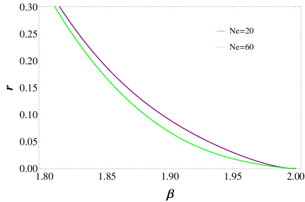
Figure 4: The variation of $r$ with $\beta$ shown for two cases studied in our model: (i) for $N=20$ when running of $n_{s}$ is considered and (ii) for $N=60$ when there is no running of $n_{s}$.

5.3.1 Power Law Starobinsky Model from No-scale SUGRA

In this section we show that the power law Starobinsly model (higher order curvature theory) can be motivated from SUGRA as they arise naturally in this framework. The SUGRA embedding of the Higgs-inflation Bezrukov does not produce a slow-roll potential in MSSM but a potential suitable for inflation is obtained in N(ext)MSSM Einhorn:2009bh . The potential in NMSSM however has a tachyonic instability in the direction orthogonal to the slow-roll Ferrara:2010yw . This instability can be cured by the addition of quartic terms of the fields in the Kähler potential Lee:2010hj ; Ferrara:2010in (see also Girish2016PLB ). In the context of a SUGRA embedding of the Starobinsky model, it was shown that quadratic Ricci curvature terms can be derived in SUGRA by adding two chiral superfields in the minimal SUGRA Cecotti:1987sa . A no-scale SUGRA model Ellis:1984bm ; Lahanas:1986uc with a modulus field and the inflation field with a minimal Wess-Zumino superpotential gives the same F-term potential in the Einstein frame as the Starobinsky model Ellis:2013xoa . The symmetry principle which can be invoked for the SUGRA generalization of the Starobinsky model is the spontaneous violation of superconformal symmetry. The quadratic curvature can also arise from D-term in a minimal-SUGRA theory with the addition of a vector and chiral supermultiplets Cecotti:1987qe . The Starobinsky model has been derived from the D-term potential of a SUGRA model Buchmuller:2013zfa . Quartic powers of Ricci curvature in the bosonic Lagrangian can also be obtained in a SUGRA model by the D-term of higher order powers of the field strength superfield Ferrara:2013kca .

More specifically, to get a no-scale SUGRA model corresponding to power law Starobinsky model which can give a larger $r$, we choose the minimal Wess-Zumino form of the superpotential (4.45) and a minimal no-scale Kähler potential with an added $(\phi+\phi^{*})^{n}$ term as

$$K=-3\ln\left[T+T^{*}-\frac{(\phi+\phi^{*})^{n}}{12}\right]$$ (5.76)

which can be motivated by a shift symmetry

$$T\rightarrow T+iC\,,\quad\phi\rightarrow\phi+iC\,,$$

with $C$ real, on the Kähler potential. Here $T$ is a modulus field and $\phi$ is a matter filed which plays the role of inflaton. We assume that the $T$ field gets a vev $\langle T+T^{*}\rangle=2\langle ReT\rangle=c>0$ and $\langle ImT\rangle=0$. We write $\phi$ in terms of its real and imaginary parts $\phi=\phi_{1}+i\phi_{2}$. If we fix the imaginary part of the inflaton field $\phi$ to be zero then $\phi=\phi^{*}=\phi_{1}$ and for simplicity we replace $\phi_{1}$ by $\phi$, the effective Lagrangian in the Einstein frame is given by

$${\cal{L}}_{E}=\frac{n(2\phi)^{n-2}[c(n-1)+\frac{(2\phi)^{n}}{12}]}{4[c-\frac{(2\phi)^{n}}{12}]^{2}}\left|\partial_{\mu}\phi\right|^{2}-\frac{4(2\phi)^{2-n}}{n(n-1)[c-\frac{(2\phi)^{n}}{12}]^{2}}\left|\frac{\partial{W}}{\partial{\phi}}\right|^{2}.$$ (5.77)

To make the kinetic term canonical in the ${\cal{L}}_{E}$, we redefine the field $\phi$ to $\chi$ with

$$\frac{\partial\chi}{\partial\phi}=-\frac{\sqrt{n(2\phi)^{n-2}[c(n-1)+\frac{(2\phi)^{n}}{12}]}}{2[c-\frac{(2\phi)^{n}}{12}]}$$ (5.78)

Assuming that $n\sim\mathcal{O}(1)$ and the large field limit $(2\phi)^{n}\gg 12c$ during inflation, integrating Eq. (5.78) gives

$$\phi\simeq\frac{1}{2}\exp\left(\frac{2\chi}{\sqrt{3n}}\right)\left[1+\frac{6c(n+1)}{n}\exp\left(\frac{-2n\chi}{\sqrt{3n}}\right)\right]$$ (5.79)

Substituting from (5.110) and (5.79) into the potential term of (5.77) and simplifying, one derives the effective scalar potential in the EF

$$V = \frac{144\mu^{2}}{n(n-1)}\left[1-\frac{2\mu}{\lambda}\exp\left(\frac{-2\chi}{\sqrt{3n}}\right)-\frac{9c(n^{2}-n-2)}{n}\exp\left(\frac{-2n\chi}{\sqrt{3n}}\right)\right]^{2}\times$$

$$\times\exp\left[\frac{2\chi}{\sqrt{6}}\left(\frac{3\sqrt{2}(2-n)}{\sqrt{n}}\right)\right]\,,$$

which, assuming $1<n<2$, in the large field limit $\chi\gg\frac{\sqrt{3n}}{2}$ is equivalent to

$$V\simeq\frac{144\mu^{2}}{n(n-1)}\exp\left[\frac{2\chi}{\sqrt{6}}\left(\frac{3\sqrt{2}(2-n)}{\sqrt{n}}\right)\right]\,.$$ (5.81)

In the limit $n\rightarrow 2$ and with the specific choice $\frac{\lambda}{\mu}=\frac{1}{2}$, the potential (5.3.1) reduces to Starobinsky Model potential. We can now compare the power law potential (5.72) and SUGRA potential (5.81) for inflaton to show the relation between the parameters of the two model. Comparing the constant coefficient and exponent in the two potentials we get

$$\beta = \frac{2\sqrt{n}+3\sqrt{2}(2-n)}{\sqrt{n}+3\sqrt{2}(2-n)}\,,$$ (5.82)

$$M^{2} = \frac{\beta^{\beta}}{6}\left[\frac{288\mu^{2}}{n(n-1)(\beta-1)}\right]^{\beta-1}\,.$$

Numerically we evaluate the SUGRA model parameter values (in $M_{p}=1$ unit) for three values of $\beta$ corresponding to running and without running of spectral index $n_{s}$ as depicted in Fig.6 and for Starobinsky limit $\beta=2$. These values are shown in the TABLE 3.

Table 3: The SUGRA model parameter values (in $M_{p}=1$ unit) for three values of $\beta$ corresponding to running and without running of spectral index $n_{s}$ as depicted in Fig.6 and for Starobinsky limit $\beta=2$.

$\beta$	$\ M$	$n$	$\mu=\frac{|\lambda|}{2}$	$\alpha_{s}=\frac{dn_{s}}{d\ln{k}}$
1.83	$1.7\times 10^{-4}$	$1.93$	$3.13\times 10^{-6}$	$-9.16\times 10^{-6}$
1.88	$1.7\times 10^{-4}$	$1.96$	$5.54\times 10^{-6}$	$-2.86\times 10^{-3}$
2.00	$1.1\times 10^{-5}$	$2.00$	$1.16\times 10^{-6}$	$-5.23\times 10^{-4}$

To summarize, this power law model with $\frac{1}{M^{2}}R^{\beta}$ correction to Einstein gravity is a generalisation of the Starobinsky model of inflation. The interesting feature of this form of generalization is that small deviations from the Starobinsky limit $\beta=2$ can change the value of tensor-to-scalar ratio from $r\sim\mathcal{O}(10^{-3})$ to $r\sim\mathcal{O}(0.1)$. We find that this model predicts large tensor-to-scale $r\approx 0.22$ as indicated by BICEP2 measurements, for the value of $\beta\approx 1.83$ and $M\sim 10^{-4}$. Also we showed that the general $R^{\beta}$ model can be obtained from a SUGRA construction with minimal Wess-Zumino form of superpotential and by adding a power law $(\phi+\bar{\phi})^{n}$ term to the minimal no-scale SUGRA Kähler potential. We further showed that this two parameter power law generalization of the Starobinsky model is equivalent to generalized non-minimal curvature coupled models with quantum corrected $\lambda\phi^{4}$ potentials $i.e.$ models of the form $\xi\phi^{a}R^{b}+\lambda\phi^{4(1+\gamma)}$, and thus the power law Starobinsky model is the most economical parametrization of such models. Since such a power law correction to Einstein gravity generates large amplitude of gravity waves, therefore they are ruled out by the current status of the observations by Planck and BKP Collaboration.

5.4 The model with two scalar fields

In this section we discuss a two-field inflationary model where the inflaton field $\phi$ is assisted by a dilaton field $\sigma$ and has a non-canonical kinetic term due to the presence of a dilaton field. Supergravity theories which are low energy limit of string theory contains several scalar fields which can be of cosmological interest. The action of the model can be generically written as

$$S = \frac{1}{2}\int d^{4}x\sqrt{-g}\left[R-\nabla^{\mu}\sigma\nabla_{\mu}\sigma-e^{-\gamma\sigma}\nabla^{\mu}\phi\nabla_{\mu}\phi-2e^{-\beta\sigma}V(\phi)\right],$$ (5.83)

where $\beta$ and $\gamma$ are arbitrary independent parameters. Brans-Dicke (BD) gravity in Einstein frame (EF) is a special case where $\beta=2\gamma$ Brans:1961sx ; Starobinsky:1994mh ; GarciaBellido:1995fz ; DiMarco:2002eb ; Gong:1998nf . However BD gravity predicts $r$ larger than the observed limit, therefore generalization of BD theory is necessary for application to inflation. In this paper we generalize the BD theory in EF to a two-parameter scalar-tensor theory where we treat $\beta$ and $\gamma$ as two independent arbitrary parameters. Addition of one extra parameter allows us to obtain viable inflation with otherwise ruled out quadratic and quartic potentials as we can have tensor-to-scalar ratio $r$ in the range of interest for forthcoming experiments.

To note, it was shown by Ellis et al. Ellis:2013xoa that the inflaton field accompanied by a moduli field $T$, which appear in string theories and have a no-scale supergravity form, give a potential for inflation equivalent to the $R+R^{2}$ Starobinsky model, producing $r\sim 10^{-3}$. We show in this paper that the above mentioned two parameter scalar-tensor theory can be obtained from no-scale supergravity theories  Cremmer:1983bf ; Ellis:1983sf ; Lahanas:1986uc which now can produce $r$ much larger than $10^{-3}$ and thus are observationally falsifiable by future experiments. Also in contrast to the supergravity embedding of the Starobinsky model, studied in Kallosh:2014qta ; Hamaguchi:2014mza , where the imaginary part of the superfield $T$ $(i.e.$ axion $\phi)$ decreases rapidly and its real part $(i.e.$ dilaton $\sigma)$ drives the inflation, we will see that in our model dilaton-axion pair evolves sufficiently during inflation and the axion acts as the inflaton.

First we look at the background dynamics of our model. Starting from the action (5.83), the equations of motion of the fields $\phi$ and $\sigma$ and the Friedmann equations can be obtained as

$$\ddot{\sigma}+3H\dot{\sigma}+\frac{\gamma}{2}e^{-\gamma\sigma}\dot{\phi}^{2}-\beta e^{-\beta\sigma}V(\phi)=0,$$ (5.84)

$$\ddot{\phi}+3H\dot{\phi}-\gamma\dot{\sigma}\dot{\phi}+e^{(\gamma-\beta)\sigma}V^{\prime}(\phi)=0,$$ (5.85)

$$3H^{2}=\frac{1}{2}\dot{\sigma}^{2}+\frac{1}{2}e^{-\gamma\sigma}\dot{\phi}^{2}+e^{-\beta\sigma}V(\phi),$$ (5.86)

$$\dot{H}=-\frac{1}{2}\left(\dot{\sigma}^{2}+e^{-\gamma\sigma}\dot{\phi}^{2}\right),$$ (5.87)

where an over dot represents derivatives w.r.t. time and prime denotes derivative with respect to $\phi$. In the slow-roll regime when both the fields slow-roll, terms with double time derivatives can be neglected and therefore the background equations reduce to

$$3H\dot{\sigma}=\beta e^{-\beta\sigma}V(\phi),~{}~{}~{}~{}~{}~{}~{}3H\dot{\phi}=-e^{(\gamma-\beta)\sigma}V^{\prime}(\phi),$$ (5.88)

$$3H^{2}=e^{-\beta\sigma}V(\phi),~{}~{}~{}~{}~{}~{}~{}~{}~{}\dot{H}=-\frac{\dot{\sigma}^{2}+e^{-\gamma\sigma}\dot{\phi}^{2}}{2}.$$ (5.89)

Here the full potential $W(\sigma,\phi)\equiv e^{-\beta\sigma}V(\phi)$ can be regarded as the product of potentials of the individual fields, $U(\sigma)\equiv e^{-\beta\sigma}$ and $V(\phi)$, and thus we define the slow-roll parameters for both the fields in a usual way (following GarciaBellido:1995fz ) :

$$\epsilon_{\phi} \equiv \frac{1}{2}\left(\frac{V^{\prime}(\phi)}{V(\phi)}\right)^{2},~{}~{}~{}~{}~{}~{}~{}~{}~{}~{}~{}~{}\eta_{\phi}\equiv\frac{V^{\prime\prime}(\phi)}{V(\phi)},$$

$$\epsilon_{\sigma} \equiv \frac{1}{2}\left(\frac{U_{\sigma}}{U}\right)^{2}=\frac{\beta^{2}}{2},~{}~{}~{}~{}~{}~{}~{}~{}\eta_{\sigma}\equiv\frac{U_{\sigma\sigma}}{U}=\beta^{2},$$ (5.90)

where $U_{\sigma}\equiv\partial U/\partial\sigma$. To ensure the smallness of the slow-roll parameters we demand that the Hubble slow-roll parameter $\epsilon_{H}\equiv-\frac{\dot{H}}{H^{2}}\ll 1$ during inflation. We notice that

$$\epsilon_{H}=\epsilon_{\sigma}+e^{\gamma\sigma}\epsilon_{\phi},$$ (5.91)

which implies that $\epsilon_{\sigma}\ll 1$ and $e^{\gamma\sigma}\epsilon_{\phi}\ll 1$ during inflation. Again, taking a time-derivative of the second equation of (5.88) to obtain $\dot{H}$, one obtains $\epsilon_{H}=\frac{\ddot{\phi}}{H\dot{\phi}}+e^{\gamma\sigma}\eta_{\phi}-(\gamma-\beta)\beta$, which implies that $e^{\gamma\sigma}\eta_{\phi}\ll 1$ and $\gamma\ll\beta+\frac{1}{\beta}\sim\frac{1}{\beta}$ (as $\beta$ is to be taken smaller than unity). We would show later on that the dilaton field $\sigma$ evolve slower than the inflaton field $\phi$ throughout the inflationary phase which would enable us to treat $\sigma$ as a background field.

Furthermore, we would require the initial field values to calculate the inflationary observables such as $n_{s}$, $r$ and $f_{\rm NL}$. From the first equation of (5.89), we notice that

$$\sigma = \sigma_{0}+\beta\ln\left(\frac{a}{a_{0}}\right),$$ (5.92)

$$\int d\phi\frac{V(\phi)}{V^{\prime}(\phi)} = -\frac{e^{\gamma\sigma_{0}}}{\beta\gamma}\left[\left(\frac{a}{a_{0}}\right)^{\beta\gamma}-1\right],$$ (5.93)

where subscript $0$ indicates the values of the quantities 60 e-foldings prior to end of inflation. Defining $f(\phi)\equiv\int d\phi\frac{V(\phi)}{V^{\prime}(\phi)}$ and requiring $\frac{a_{f}}{a_{0}}\gtrsim e^{\Delta N}$ (subscript $f$ denoting the quantities at the end of inflation) for sufficient inflation, one gets

$$\frac{1}{\beta\gamma}\ln\left[1+\beta\gamma e^{-\gamma\sigma_{0}}(f(\phi_{0})-f(\phi_{f}))\right]\gtrsim\Delta N.$$ (5.94)

The perturbation analysis of such a model has been extensively discussed in Starobinsky:1994mh ; GarciaBellido:1995fz ; DiMarco:2002eb , where the comoving curvature perturbation is defined as

$$\hskip-8.5359pt\mathcal{R}=\Phi-\frac{H}{\dot{H}}\left(\dot{\Phi}+H\Phi\right)=\Phi+H\frac{\dot{\sigma}\delta\sigma+e^{-\gamma\sigma}\dot{\phi}\delta\phi}{\dot{\sigma}^{2}+e^{-\gamma\sigma}\dot{\phi}^{2}},$$ (5.95)

where $\Phi$ is the scalar metric perturbation in the longitudinal gauge. As we are dealing with a multi-field inflationay model, $\mathcal{R}$ is not a frozen quantity on superhorizon scales and its time evolution is given by

$$\mathcal{\dot{R}}=\frac{k^{2}}{a^{2}}\frac{H^{2}}{\dot{H}}\Phi+\mathcal{S},$$ (5.96)

where $\cal{S}$ represents isocurvature (or entropy) perturbations given by

$$\hskip-8.5359pt\mathcal{S}=\frac{2H(\beta\dot{\sigma}\dot{\phi}^{2}V(\phi)e^{-\gamma\sigma}+\dot{\phi}\dot{\sigma}^{2}V^{\prime}(\phi))}{e^{\beta\sigma}(\dot{\sigma}^{2}+e^{-\gamma\sigma}\dot{\phi}^{2})^{2}}\left(\frac{\delta\sigma}{\dot{\sigma}}-\frac{\delta\phi}{\dot{\phi}}\right).$$ (5.97)

Under slow-roll approximation, one can solve for the scalar perturbations of the model, $\delta\sigma$, $\delta\phi$ and $\Phi$, on superhorizon scales, which turn out to be Starobinsky:1994mh

$$\hskip-19.91684pt\frac{\delta\sigma}{\dot{\sigma}} = \frac{c_{1}}{H}-\frac{c_{3}}{H}\,;~{}~{}~{}~{}~{}~{}~{}~{}~{}~{}~{}\frac{\delta\phi}{\dot{\phi}}=\frac{c_{1}}{H}+\frac{c_{3}}{H}\left(e^{-\gamma\sigma}-1\right),$$ (5.98)

$$\hskip-19.91684pt\Phi = -c_{1}\frac{\dot{H}}{H^{2}}+c_{3}\left[\frac{1}{2}\left(\frac{V^{\prime}(\phi)}{V(\phi)}\right)^{2}\left(1-e^{\gamma\sigma}\right)-\frac{\beta^{2}}{2}\right],$$ (5.99)

where $c_{1}$ and $c_{3}$ are the time independent integration constants and can be fixed using initial conditions. In the above expression (5.99), terms proportional to $c_{1}$ represent the adiabatic modes while those proportional to $c_{3}$ represent the isocurvature modes. Using eq.s (5.88)-(5.90), the comoving curvature perturbation (5.95) can be simplified to the form: ${\mathcal{R}}\simeq\Phi+c_{1}-c_{3}+c_{3}\epsilon_{\phi}(\epsilon_{\sigma}+e^{\gamma\sigma}\epsilon_{\phi}).$

Since from eq.(5.99), it is clear that all the terms in $\Phi$ are proportional to $(c_{1},c_{3})\times$ slow-roll parameters, therefore we will ignore the potential $\Phi$ compared to $c_{1}$ and $c_{3}$ in ${\mathcal{R}}$. From eq. (5.98), we can calculate $c_{1}$ and $c_{3}$. Substituting $c_{1}$ and $c_{3}$, the comoving curvature perturbation on super horizon scales becomes

$${\mathcal{R}}=H\frac{\delta\phi}{\dot{\phi}}e^{\gamma\sigma}A+H\frac{\delta\sigma}{\dot{\sigma}}B,$$ (5.100)

where $A=\epsilon_{\phi}/\epsilon_{H}$ and $B=\epsilon_{\sigma}/\epsilon_{H}$.

Now we look at the observables predicted by this model. The mode functions for superhorizon fluctuations of $\sigma$ and $\phi$, evaluated at horizon crossing $k=a(t_{k})H(t_{k})$, are $\langle|\delta\sigma(k)|^{2}\rangle=H^{2}(t_{k})/2k^{3}$ and $\langle|\delta\phi(k)|^{2}\rangle=e^{\gamma\sigma(t_{k})}H^{2}(t_{k})/2k^{3}$. Therefore, the power spectrum of comoving curvature perturbations becomes

$${\mathcal{P}}_{\mathcal{R}}\equiv\frac{k^{3}}{2\pi^{2}}\langle{\mathcal{R}}^{2}\rangle=\frac{H^{2}}{8\pi^{2}\epsilon_{H}}.$$ (5.101)

The tensor power spectrum retains its generic form, because the action involves only minimal Einstein curvature term $R$, given by $\mathcal{P}_{\mathcal{T}}=8H^{2}(t_{k})/4\pi^{2}$, which yields the tensor-to-scalar ratio as

$$r\equiv\frac{\mathcal{P}_{\mathcal{T}}}{\mathcal{P}_{\mathcal{R}}}=16\epsilon_{H}.$$ (5.102)

The scalar spectral index $n_{s}$ in this model is

$$\hskip-8.5359ptn_{s}-1\simeq A\left[(2\eta_{\phi}-6\epsilon_{\phi})e^{2\gamma\sigma}-\beta(2\beta+\gamma)e^{\gamma\sigma}\right]-B\beta^{2}.$$ (5.103)

It can be noted that in the limit $\beta\rightarrow 0$ and $\gamma\rightarrow 0$ (i.e. $A=1$ and $B=0$) the forms of power spectrum, tensor-to-scalar ratio and spectral index reduce to their standard forms in the single field slow-roll inflation.

It is important to note that in our model the amplitude of the isocurvature perturbations,

$$\hskip-5.69046pt{\mathcal{P}}_{\mathcal{S}}=\frac{k^{3}}{2\pi^{2}}\langle{\mathcal{S}}^{2}\rangle=\frac{H^{4}}{\pi^{2}}\frac{\left[\beta e^{-\gamma\sigma}\dot{\phi}V(\phi)+\dot{\sigma}V^{\prime}(\phi)\right]^{2}}{e^{(2\beta-\gamma)\sigma}(\dot{\sigma}^{2}+e^{-\gamma\sigma}\dot{\phi}^{2})^{3}},$$ (5.104)

vanishes in the slow-roll approximation (using (5.88)). The multifield models with non-canonical kinetic term posses a strong single-field attractor solution Kaiser:2013sna ; Schutz:2013fua as has also been observed in this case. But generally these multifield models produce isocurvature perturbations which can also account for a large angular scale suppression of the power spectrum. But our case differs from such multifield models as it does not produce any isocurvature perturbations upto slow-roll approximation.

5.4.1 Analysis of the Model with $\lambda_{n}\phi^{n}$ Potentials

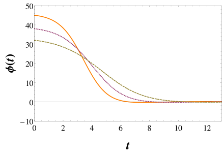
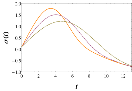
Figure 5: Evolution of the scalar fields w.r.t. time $t$ measured in the units of $m_{\phi}^{-1}$ is shown.

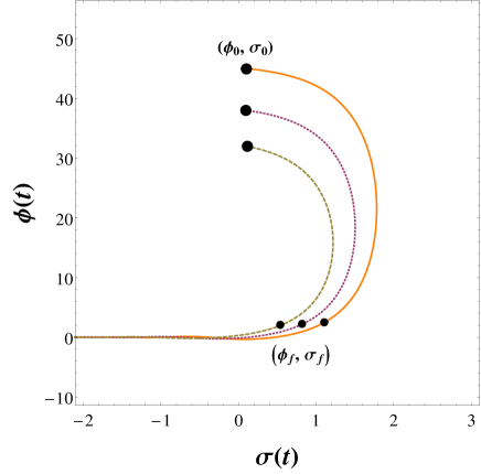
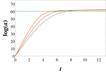
Figure 6: Upper panel : Evolution of the inflaton $\phi(t)$ with respect to dilaton $\sigma(t)$ is shown. Bigger black dots correspond to the field values when inflation starts and smaller dots correspond to the field values at the end of inflation. We see that during inflation the evolution of dilaton is much slower compared to inflaton. Lower panel : The cosmological evolution of the scale factor is shown. The straight dot-dashed line represent the $\Delta N=60$ line where inflation ends.

In this model, we treat the $\phi$ field as the inflaton field which is assisted by the dilaton field $\sigma$ during the inflationary evolution. This can only be ensured if we confirm that the $\sigma$ field evolves slower than the $\phi$ field during the entire inflationary epoch. To show this, we first study the background evolution of both the scalar fields $\phi$ and $\sigma$ by numerically solving the field eq.s (5.84-5.87). We first treat the case when the inflaton field has quadratic potential $V(\phi)=m_{\phi}^{2}\phi^{2}/2$. As some representative initial conditions, we choose $\sigma_{0}=0.1$ and $\phi_{0}=45$ (Solid), $\phi_{0}=38$ (Dotted), $\phi_{0}=32$ (Dashed) corresponding to $\beta=0.04$, $\beta=0.035$, $\beta=0.03$ respectively. Also we fix $\gamma=2\sqrt{2/3}$ for each case, which is required for the SUGRA derivation of this model studied in the later part of this paper. The initial conditions are chosen carefully such that we get correct $n_{s}$ and $r$ for $\Delta N\simeq 60$ e-folds. In FIG. 5, we show the time evolution of the fields $\phi$ and $\sigma$ where time is given in the units of $m_{\phi}^{-1}$. The different colors in the figure correspond to different initial conditions as described above. In FIG. 6 (upper panel) shows the evolution of the fields in $(\sigma,\phi)$ plane. This plot shows that during $60$-efolds inflation, dilaton $\sigma$ evolves much slower compared to inflaton $\phi$. After the end of inflation, inflaton goes to its minimum value $\phi=0$. Such background evolution of the fields also ensure that the background spatial metric evolves (quasi-)exponentially during inflation which has been depicted in the lower panel of FIG. 6. Also we checked that for the case of quartic potential $V(\phi)=\lambda\phi^{4}/4$, the fields evolve in a similar way ensuring that $\phi$ can be treated as an inflaton field.

We now analyze the observable parameters for inflaton potential $V(\phi)=\lambda_{n}\phi^{n}/n$. From eq. (5.93), we find $\sigma_{f}=\sigma_{0}+\beta\Delta N$. Using $\epsilon_{H}=1$, which is the condition for the end of inflation, we obtain $\phi_{f}=ne^{\gamma\sigma_{f}/2}/\sqrt{2-\beta^{2}}$. From eq.(5.94), the field value $\phi_{0}$ can be expressed in terms of $\phi_{f}$ and $\sigma_{0}$ as $\phi_{0}^{2}\simeq\phi_{f}^{2}+\frac{2n}{\beta\gamma}e^{\gamma\sigma_{0}}\left(e^{\beta\gamma\Delta N}-1\right).$

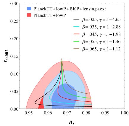
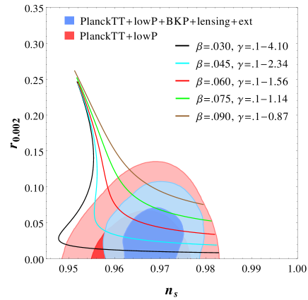
Figure 7: The $n_{s}-r$ predictions of the model for quadratic (upper panel) and quartic (lower panel) potentials are shown with various contour lines and compared with $1\sigma$ and $2\sigma$ contours of the Planck observations Ade:2015xua . We take $\Delta N=60$ and $\sigma_{0}=0.1$. In both the figures the range of values of $\gamma$ increases along the curves from top to bottom. It is also manifest that as the values of $\beta$ and $\gamma$ goes to zero, $n_{s}$ and $r$ values converges to standard slow-roll inflation predictions.

Now we substitute $\phi_{0}$ into eq.s (5.101), (5.102) and (5.103) to give $n_{s}$, $r$ and ${\mathcal{P}}_{\mathcal{R}}$ in terms of $\sigma_{0}$, $n$, $\Delta N$, $\beta$ and $\gamma$. For $\Delta N=60$ e-folds and for the choice $\sigma_{0}=0.1$ with various choices of the parameters $\beta$ and $\gamma$, the $n_{s}-r$ predictions for quadratic $(n=2)$ and quartic $(n=4)$ potentials are shown in the FIG. 7. For $\sigma_{0}=0.1$, $\Delta N=60$ and for the range of the parameter values of ($\beta,\gamma$) as shown in FIG. 7, we find inflaton mass in the range $\lambda_{2}=m_{\phi}^{2}\sim 10^{-11}-10^{-14}$ and self-coupling in the range $\lambda_{4}=\lambda\sim 10^{-13}-10^{-17}$. E.g. for the choice $\beta=0.05$, $\gamma=0.7$, which can produce $n_{s}\simeq 0.9666$, $r\simeq 0.06$, gives $m_{\phi}\approx 2\times 10^{-6}$. And for $\beta=0.06$, $\gamma=1$, which produces $n_{s}\simeq 0.964$, $r\simeq 0.05$, gives $\lambda\approx 10^{-16}$. Therefore, in this model with quadratic and quartic potentials, similar to the case of single-field slow-roll inflation, we require light inflaton mass and fine-tuning of the inflaton self-coupling in order to fit the observed CMB amplitude. However, unlike the Higgs inflation which predicts very small $r\approx 0.003$ and standard single-field inlation with quadratic and quartic potentials give large $r$, the two field model can give $r$ close to the present bound $r<0.07$. For the above mentioned initial conditions, coupling constants and parameter values, the running of the spectral index $\alpha_{s}\equiv\frac{dn_{s}}{d\ln k}\simeq\frac{1}{H}\frac{dn_{s}}{dt}$ comes out to be $\alpha_{s}\simeq-6.7\times 10^{-4}$ and $\alpha_{s}\simeq-1.2\times 10^{-3}$ for quadratic and quartic potentials, respectively, fully consistant with the Planck observation $\alpha_{s}=−0.0084\pm 0.0082~{}(68\%CL,PlanckTT+lowP)$ Ade:2015lrj .

Finally, we notice that this model yields negligible non-Gaussianity (up to slow-roll approximation). This can be seen as follows. Let us first note that besides yielding $r$, $n_{s}$ and $\alpha_{s}$ within the observational bounds, a viable inflationary model should not produce large Non-Gaussianity (NG) to remain in accordance with observations. NG in multifield models where the fields have non-canonical kinetic terms has been calculated in Ref.s Seery:2005gb ; Choi:2007su . Following these Ref.s, we calculated the non-linearity parameter $f_{NL}$ which characterizes the amplitude of NG. We find that for the range of parameters values as shown in FIG. 5, $f_{NL}\sim\mathcal{O}(10^{-2})-\mathcal{O}(10^{-3})$ consistent with the observations. Also we find that $f_{NL}$ does not depend on initial value of the dilaton $\sigma_{0}$ and coupling constants for the considered chaotic form of potential.

The NG parameter $f_{NL}$ is given as

$$-\frac{5}{6}f_{NL}\equiv-\frac{5}{6}f_{NL}^{(3)}-\frac{5}{6}f_{NL}^{(4)}.$$ (5.105)

If one writes the multifield action as

$$S=\frac{1}{2}\int d^{4}x\sqrt{-g}\left[R-G_{IJ}\partial_{\mu}\varphi^{I}\partial^{\mu}\varphi^{J}-2W(\varphi)\right],$$ (5.106)

then it is shown in Seery:2005gb that the Bispectrum non-Gauassian parameter $f_{NL}$ is

$$-\frac{5}{6}f_{NL}N_{,MN}{(N_{,I}N_{,J}G^{IJ})^{2}}=-\frac{5}{6}f_{NL}^{(3)}-\frac{5}{6}f_{NL}^{(4)}\,.$$ (5.107)

Following Choi:2007su one gets

$$-\frac{5}{6}f_{NL}^{(3)}=\frac{r}{16}(1+f)$$ (5.108)

where

$$f\equiv-1-\frac{1}{2\displaystyle\sum_{i}k_{i}^{3}}\displaystyle\sum_{\rm perms}\left[-3\frac{k_{2}^{2}k_{3}^{2}}{k_{t}}-\frac{k_{2}^{2}k_{3}^{2}}{k_{t}^{2}}(k_{1}+2k_{3})+\frac{1}{2}k_{1}^{3}-k_{1}k_{2}^{2}\right],$$

$$k_{t}=\displaystyle\sum_{i}k_{i}\,,$$

$$-\frac{5}{6}f_{NL}^{(4)}=\frac{2}{\left[e^{\gamma\sigma_{*}}\frac{v^{2}}{\epsilon_{\phi}^{*}}+\frac{u^{2}\alpha^{2}}{\epsilon_{\sigma}^{*}}\right]^{2}}\left[\frac{u^{3}\alpha^{3}}{\epsilon_{\sigma}^{*}}\left(1-\frac{\eta_{\sigma}^{*}}{2\epsilon_{\sigma}^{*}}\right)+e^{2\gamma\sigma^{*}}\frac{v^{3}}{\epsilon_{\phi}^{*}}\left(1-\frac{\eta_{\phi}^{*}}{2\epsilon_{\phi}^{*}}\right)-\right.$$

$$\left.-\frac{u^{2}\alpha^{2}v}{(2\epsilon_{\sigma}^{*})^{\frac{1}{2}}\epsilon_{\sigma}^{*}}\gamma e^{\gamma\sigma_{*}}-\left(\frac{u\alpha}{\epsilon_{\sigma}^{*}}-\frac{v}{\epsilon_{\phi}^{*}}\right)^{2}e^{2\gamma\sigma_{*}}\mathcal{A}_{P}\right],\\$$

where $*$ denotes the quantities at horizon crossing,

$$u\equiv\frac{\epsilon_{\sigma}^{f}}{\epsilon^{f}}\,,\quad v\equiv\frac{\epsilon_{\phi}^{f}}{\epsilon^{f}}\,,\quad\alpha\equiv 1+\left(e^{\gamma\sigma_{f}}-e^{\gamma\sigma_{*}}\right)\frac{\epsilon_{\phi}^{f}}{\epsilon_{\sigma}^{f}}\,,$$

$$\mathcal{A}_{P}=-\frac{\epsilon_{\sigma}^{f}\epsilon_{\phi}^{f}}{\epsilon^{f^{2}}}\left[\eta_{ss}^{f}+\frac{\gamma e^{\gamma\sigma_{f}}\epsilon_{\phi}^{f^{2}}}{\sqrt{2\epsilon_{\sigma}^{f}}\epsilon^{f}}-\frac{4\epsilon_{\sigma}^{f}\epsilon_{\phi}^{f}}{\epsilon_{f}}\right]\,,$$

$$\eta_{ss}\equiv\frac{\eta_{\phi}\epsilon_{\sigma}+\eta_{\sigma}\epsilon_{\phi}}{\epsilon}\,.$$

This model is a multifield model where the inflaton has a non-canonical kinetic term. Multifield inflation with canonical kinetic terms generically yields a local NG which is peaked in the squeezed configuration ($k_{3}\ll k_{1},\,k_{2}$), whereas multifield inflation with non-canonical kinetic term of inflaton yields NG of equilateral type ($k_{1}=k_{2}=k_{3}$) Ade:2015lrj . We see that the momentum dependent factor $f$ in (5.4.1) yields 0 and 5/6 for squeezed and equilateral configuration respectively, and numerically find that for any choice of parameter values which give correct $n_{s}$ and $r$ produce the Non-Gaussianity peaking in the equilateral configuration. This indicates, that despite having two fields, the model behaves like a single-field model with non-canonical kinetic term.

5.4.2 Two-Field Model Action from No-scale Supergravity

In this section we show that, such a two-field inflationary model can be realised in the realm of no-scale Supergravity. The two-field models of inflation with string motivated tree-level no-scale Kähler potential in no-scale supergravity framework are analyzed in Casas:1998qx ; Ellis:2014gxa ; Ferrara:2014ima ; Ellis:2014opa . We consider the Kähler potential of the following form

$$K=-3\ln[T+T^{\ast}]+\frac{b\rho\rho^{\ast}}{(T+T^{\ast})^{\omega}},$$ (5.109)

here $T$ is the two component chiral superfield whose real part is the dilaton and imaginary part is an axion. We identify axion as the inflaton of the model, and $\rho$ is an additional matter field with modular weight $\omega$. In typical orbifold string compactifications with three moduli fields, the modular weight $\omega$ has value $3$ Dixon:1989fj ; Casas:1998qx ; Ellis:2014gxa . Here we shall treat $\omega$ as a phenomenological parameter whose value can have small deviation from the canonical value $3$ which may be explained via string loop corrections to the effective supergravity action Derendinger:1991hq . In this model to obtain the correct CMB observables, the parameter $(3-\omega)$ has to be fine tuned to the order of $10^{-2}$.

For the complete specification of supergravity, we assume the superpotential as

$$W=\lambda_{m}~{}\rho~{}T^{m}.$$ (5.110)

We can decompose $T$ field in its real and imaginary parts parametrized by two real fields $\sigma$ and $\phi$, respectively, as

$$T=e^{-\sqrt{2/3}\sigma}+i\sqrt{2/3}\phi.$$ (5.111)

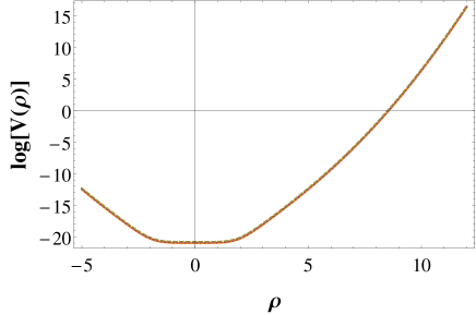
Figure 8: Inflationary evolution of the potential $V(\rho)$ is shown for the three initial condition as discussed before. We see that during inflation the potential for the field $\rho$ is exponential steep and therefore the field $\rho$ rapidly falls towards the minima of the potential and stabilizes at $\rho=0$.

The evolution of the matter field $\rho$ is constrained by the exponential factor $e^{K}$ via $e^{G}$ in the scalar potential (4.36) as $V\propto e^{\frac{b\rho\rho^{\ast}}{(T+T^{\ast})^{\omega}}}$. Since $(T+T^{\ast})^{-\omega}=2e^{\frac{2}{3}\omega\sigma}\gtrsim 2$ for $\omega\approx 3$ and $\sigma>0$ during inflation. Therefore field $\rho$, due to its exponentially steep potential, is rapidly driven to zero at the start of the inflation and stabilizes at $\rho=0$  Ellis:2014opa . In FIG. 8, we show the stabilization of the field $\rho$ for different initial conditions as discussed before for $(2m=n=2)$. We also checked the evolution of $\rho$ for $(2m=n=4)$ and found that it stabilizes in the similar fashion. Therefore for vanishing $\rho$, the scalar potential (4.36) and kinetic term (4.30) takes the simple form

$$V=\frac{\lambda_{m}^{2}T^{m}T^{\ast m}}{b(T+T^{\ast})^{3-\omega}},~{}~{}~{}~{}~{}~{}\mathcal{L}_{K}=\frac{3\partial^{\mu}T\partial_{\mu}T^{\ast}}{(T+T^{\ast})^{2}},$$ (5.112)

which upon using the decomposition of $T$ becomes

$$\mathcal{L}_{K} = \frac{1}{2}\partial^{\mu}\sigma\partial_{\mu}\sigma+\frac{1}{2}e^{-\gamma\sigma}\partial^{\mu}\phi\partial_{\mu}\phi,$$ (5.113)

$$V = \frac{2^{\omega-3}\lambda_{m}^{2}}{b}~{}e^{-\beta\sigma}\left[e^{\gamma\sigma}+\frac{2}{3}\phi^{2}\right]^{m},$$ (5.114)

where $\gamma=2\sqrt{2/3}\simeq 1.633$ and $\beta=(3-\omega)\sqrt{2/3}$. Since during inflation, dilaton $\sigma$ evolves much slower compared to inflaton $\phi$, see FIG. 6, therefore $e^{\gamma\sigma}\ll\phi^{2}$ and hence the first term inside the bracket in (5.114) can be neglected compared to second term.

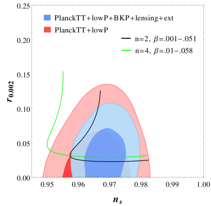
Figure 9: The $n_{s}-r$ predictions for quadratic ($n=2$) and quartic ($n=4$) potentials, with a fixed value of $\gamma=2\sqrt{2/3}$ are shown and compared with $1\sigma$ and $2\sigma$ contours of the Planck observations Ade:2015xua . The range of values of $\beta$ increases along the curves from top to bottom.

Therefore, from (5.113) and (5.114), the Lagrangian in EF becomes

$$\mathcal{L}_{M}=\frac{1}{2}\partial^{\mu}\sigma\partial_{\mu}\sigma+\frac{1}{2}e^{-\gamma\sigma}\partial^{\mu}\phi\partial_{\mu}\phi+e^{-\beta\sigma}V(\phi),$$ (5.115)

where $V(\phi)=\lambda_{m}^{2}\phi^{2m}/2m$ and we set $b=2^{\omega}/6$ for quadratic potential ($2m=n=2$) and $b=2\times 2^{\omega}/9$ for quartic potential ($2m=n=4$). We see that the parameter $b$ is no new parameter and can be given in terms of $\omega$. For $\Delta N=60$ and $\sigma_{0}=0.1$, the $n_{s}-r$ predictions for a fixed value of $\gamma=2\sqrt{2/3}$ and with varying $\beta$ are shown in FIG. 9.

To summarize, this two-field two-parameter inflationary model, where the inflaton field has a non-canonical kinetic term due to the presence of the dilaton field, renders quartic and quadratic potentials of the inflaton field viable with current observations. Unlike Higgs-inflationary scenario which predicts very small tensor-to-scalar ratio $r\approx 0.003$, this model can produce large $r$ in the range $r\sim 10^{-1}-10^{-2}$ which would definitely be probed by future $B-$mode experiments and thus such a model can be put to test with the future observations. Also this model produces no isocurvature perturbations upto slow-roll approximation and predicts negligible non-Gaussianity consistent with the observations. In addition, we showed that this model can be obtained from a no-scale SUGRA model which makes this model of inflation phenomenologically interesting from the particle physics perspective.

6 Conclusions

The idea, that the universe through a period of exponential expansion, called inflation, has proved useful for solving the horizon and flatness problems of standard cosmology and in addition providing an explanation for the scale invariant super-horizon perturbations which are responsible for generating the CMB anisotropies and formation of structures in the universe. A successful theory of inflation requires a flat potential where a scalar field acquires a slow-roll over a sufficiently long period to enable the universe to expand by at least $60$ e-foldings during the period of inflation.

There are a wide variety of particle physics models which can provide the slow-roll scalar field ’inflaton’ for inflation Lyth:1998xn ; Martin:2013tda . From the observations of CMB anisotropy spectrum by COBE, WMAP and Planck Smoot:1998jt ; WMAP9 ; Planck:2015 , it is not yet possible to pin down a specific particle physics model as the one responsible for inflation. Though all of the above experiments gave tighter and tighter constraints on inflationary observables, $e.g.$ power spectrum and spectral index, which allowed several models of inflation to be ruled out but still there is a large degeneracy in inflation models. The 2015 data from Planck observation gives the amplitude, spectral index and tensor-to-scalar ratio as $10^{10}\ln(\Delta_{\mathcal{R}}^{2})=3.089\pm 0.036$, $n_{s}=0.9666\pm 0.0062$ at ($68\%$ CL) and $r_{0.002}<0.11$ at ($95\%$CL), respectively Ade:2015lrj . Also the latest results by BKP collaboration put $r$ at $r_{0.05}<0.07$ at ($95\%$CL)bicep2keck2015 . Therefore, all those models which can produce the correct amplitude of CMB power spectrum and its spectral tilt along with producing $r<0.07$ are allowed. The future $B-$mode observations are expected to fix $r$ which will allow many existing inflation models to be ruled out.

In this review we have presented some recent results of a single-field generalized non-minimal model of inflation, a power law model of inflation and a two-field model of inflation with a non-canonical kinetic term. We have calculated the key inflationary observables : amplitude of the power spectrum of curvature perturbations, spectral index and its running, tensor-to-scalar ratio and amplitude of isocurvature perturbations. We fix the parameters of the models using the measured values of these observables. Also we motivate these models from a fundamental theory called no-scale supergravity. From the analysis of these models we find that the power law model $R+R^{\beta}/M^{2}$ of inflation and therefore all the models of inflation with the Lagrangian $R+\xi\phi^{a}R^{b}+\lambda\phi^{4(1+\gamma)}$ are ruled form the current bound on $r_{0.05}<0.07$ at ($95\%$CL). However for $\beta=2$ which corresponds to Starobinsky model $R+R^{2}/M^{2}$ of inflation produces $r\simeq 0.0033$. This prediction of $r\simeq 0.0033$ however very small but is currently favored by the observations. Contrary to the large $r$ prediction of power law model, the two field model predicts a range of $r\sim 10^{-1}-10^{-2}$ values close the present bound on $r$.

Currently tensor-to-scalar ratio is an extremely important inflationary parameter in view of validating and ruling out models of inflation, and therefore many models that can be classified as extended theories of gravity. The observation of primordial $B$-modes (CMB polarization) will provide the constraint on $r$. The $B$-modes are the signature of inflationary tensor modes, precise observations of which will provide a most distinctive confirmation of occurrence of an inflationary era in the early universe. There are several ongoing experiments for $B-$mode detection and all hope to observe these signals from the inflationary era. There are several experiments, $e.g.$ ground based (Keck/BICEP3, SPT-3G, AdvACT, CLASS, Simons Array), balloons based (Spider,EBEX) and satellites based (CMBPol, LiteBIRD and COrE). These observational experiments will be taking into account the recent Planck data on polarized dust. They aim to probe the tensor-to-scale ratio at the level of $r\sim 10^{-3}$ which is a theoretically motivated limit Creminelli:2015oda . High precision measurements of small-scale temperature anisotropies along with the observations of $B-$mode will not only test the inflationary hypothesis but allow to remove a large degeneracy in the models of inflation.

- (1) A.G. Reiss et al., Astron. J. 116, 1009 (1998). S. Perlmutter et al., Nature (London) 391, 51 (1998).
- (2) P.A.R. Ade et al., Plnack Coll., arXiv:1502.02114 [astro-ph.CO].
- (3) P.A.R. Ade et al., Planck Coll., arXiv:1502.01589 [astro-ph.CO].
- (4) P.A.R. Ade et al., BICEP2-Planck Coll., Phys. Rev. Lett. 114.
- (5) P.A.R. Ade et al., Keck Array and BICEP2 Coll., arXiv:1390175[astro-ph.CO].
- (6) P. A. R. Ade et al. [Planck Collaboration], arXiv:1502.01589 [astro-ph.CO].
- (7) C.M. Will, Theory and Experiment in Gravitational Physics, 2nd ed. Cambridge University Press, Cambridge, UK (1993).
- (8) L.P. Eisenhart, Riemannian Geometry, Princeton Univ. Press, Princeton, (1955).
- (9) E. Schrödinger , Space-Time Structure, Cambridge Univ. Press, Cambridge, (1960).
- (10) T. Levi-Civita, The Absolute Differential Calculus, Blackie and Son, London, 1929.
- (11) O. Klein, New Theories in Physics, 77, Intern.Inst. of Intellectual Co-operation, League of Nations, (1938).
- (12) E. Cartan, Ann. Ec. Norm. 42, 17 (1925).
- (13) A. Palatini, Rend. Circ. Mat. Palermo 43, 203 (1919).
- (14) G. Basini, S. Capozziello, Gen. Rel. Grav. 35, 2217 (2003).
- (15) M.B. Green, J.H Schwarz, E. Witten, Superstring Theory, Cambridge Univ. Press, Cambridge, (1987).
- (16) K.T. Story, et al., Astrophys. J. 779 (2013) 86.
- (17) G.F. Smoot, COBE observations and results, astro-ph/9902027.
- (18) C.L. Bennet et al., WMAP Coll., Astrophys. J. Suppl. 208, 20 (2013).
- (19) A.H. Guth, Phys. Rev. D23 (1981) 347. A.A. Starobinsky, JETP Lett. 30, 682 (1979). D. Kazanas, Astrophys. J. 241, L59 (1980). K. Sato, Mon. Not. Roy. Astron. Soc. 195, 467 (1981). A.D. Linde, Phys. Lett. B108 (1982) 389. A. Linde, Phys. Lett. B 114 (1982) 431. A. Linde, Phys. Lett. B 116 (1982) 335. A. Albrecht, and P.J. Steinhardt, Phys. Rev. Lett. 48 (1982) 1220.
- (20) A.D. Linde, Phys. Lett. B129 (1983) 177.
- (21) A.D. Linde, Phys. Lett. B108 (1982) 389.
- (22) B.A. Bassett, S. Tsujikawa, and D. Wands, Rev. Mod. Phys. 78 (2006) 537.
- (23) R. Allahverdi, R. Brandenberger, F.-Y. Cyr-Racine, and A. Mazumdar, Ann. Rev. Nucl. Part. Sci. 60 (2010) 27.
- (24) J. Martin, Ch. Ringeval, and V. Vennin, Encyclopædia Inflationaris, Phys. Dark Univ. 5-6, 75 (2014).
- (25) D. Baumann, arXiv: 0907.5424[hep-th], TASI-2009.
- (26) A. Riotto, arXiv: hep-ph/0210162”,
- (27) S. Dodelson, Modern cosmology, ACADEMIC PRESS, An Imprint of Elsevier, 2003.
- (28) J.M. Bardeen, Phys. Rev. D22 (1980) 1882.
- (29) J.M. Bardeen, P.J. Steinhardt, and M.S. Turner, Phys. Rev. D28 (1983) 679.
- (30) V.F. Mukhanov, H.A. Feldman, and R.H. Brandenberger, Phys. Rept. 215 (1992) 203.
- (31) D.I. Kaiser and A.T. Todhunter, Phys. Rev. D81 (2010) 124037.
- (32) C. Gordon, et al., Phys. Rev. D63 (2001) 023506.
- (33) V.F. Mukhanov, Physical Foundations of Cosmology, CAMBRIDGE UNIVERSITY PRESS, 2005.
- (34) S. Nojiri, S.D. Odintsov, Int. J. Geom. Meth. Mod. Phys. 4, 115 (2007). S. Capozziello and M. Francaviglia, Gen. Rel. Grav.: Special Issue on Dark Energy 40, 357 (2007).
- (35) H. Bondi, Cosmology, Cambridge Univ. Press, Cambridge, UK (1952).
- (36) N.D. Birrell, P.C.W. Davies, Phys. Rev. D 22, 322 (1980). G.A. Vilkovisky, Class. Quant. Grav. 9, 895 (1992). M. Gasperini , G. Veneziano, Phys. Lett. B 277, 256 (1992).
- (37) P. Teyssandier, P. Tourrenc, J. Math. Phys. 24, 2793 (1983). K. Maeda, Phys. Rev. D 39, 3159 (1989). D. Wands, Class. Quantum Grav. 11, 269 (1994). S. Capozziello , R. de Ritis, A.A. Marino, Gen. Relativ. Grav. 30, 1247 (1998). S. Gottlöber, H.-J. Schmidt, A.A. Starobinsky, Class. Quantum Grav. 7, 893 (1990). F. Adams, K. Freese, A. Guth, Phys. Rev. D 43, 965 (1991).
- (38) G. Magnano, L.M. Sokolowski, Phys. Rev. D 50, 5039 (1994).
- (39) A.A. Starobinsky, Phys. Lett. B 91, 99 (1980). R. Kerner, Gen. Rel. Grav. 14, 453 (1982). J.P. Duruisseau , R. Kerner, Gen. Rel. Grav. 15 797, (1983). D. La, P.J Steinhardt, Phys. Rev. Lett. 62, 376 (1989).
- (40) P.G. Bergmann, Int. J. Theor. Phys.1 (1968) 25. H.A. Buchdahl, Mon. Not. Roy. Astron. Soc. 150 (1970) 1.
- (41) A.A. Starobinsky, Phys. Lett. B 91, 99 (1980).
- (42) A. De Felice, and S. Tsujikawa, Living Rev. Rel. 13, 3 (2010).
- (43) F. Bezrukov, A. Magnin, and M. Shaposhnikov, Phys. Lett. B675 (2009) 88.
- (44) S. Capozziello, V. Faraoni, Beyond Einstein Gravity, Fundamental Theories of Physics Vol. 170, Springer Ed., Dordrecht (2011). S. Capozziello and M. De Laurentis, Phys. Rep. 509, 167 (2011). S. Nojiri and S.D. Odintsov, Phys. Rep. 505, 59 (2011).
- (45) S. Capozziello, Int. J. Mod. Phys. D 11, 483 (2002). V. Faraoni, Phys. Rev. D 74, 023529 (2006). L. Amendola, R. Gannouji, D. Polarski, and S. Tsujikawa, Phys. Rev. D 75, 083504 (2007). N. Agarwal and R. Bean, Class. Quant. Grav. 25, 165001 (2008). W. Hu and I. Sawicki, Phys. Rev. D 76, 064004 (2007). A. de la Cruz-Dombriz and A. Dobado, Phys. Rev. D 74, 087501 (2006). S. A. Appleby and R. A. Battye, Phys. Lett. B 654, 7 (2007). A. A. Starobinsky, JETP Lett. 86, 157 (2007). S. Nojiri and S. D. Odintsov, Phys. Lett. B 652, 343 (2007). B. Whitt, Phys. Lett. B 145, 176 (1984). S. Capozziello and G. Lambiase, New Adv. in Phys. 7, 13 (2013) [arXiv:1304.5640[astro-ph.CO]]. S. Capozziello, G. Lambiase, H.-J. Schmidt, Ann. of Phys. (Leipzig) 9, 39 (2000). S. Capozziello, G. Lambiase, Gen. Rel. Grav. 32, 295 (2000). S. Capozziello, G. Lambiase, Grav. and Cosm. 6, 173 (2000). S. Capozziello, G. Lambiase, Gen. Rel. Grav. 31, 1005 (1999). S. Capozziello, G. Lambiase, Gen. Rel. Grav. 32, 673 (2000). S. Capozziello, G. Lambiase, Mod. Phys. Lett. A 14, 2193 (1999). G. Lambiase, S. Mohanty, and G. Scarpetta, JCAP0807 (2008) 019. G. Lambiase, M. Sakellariadou, and A. Stabile, JCAP 1312 (2013) 020. G. Lambiase, G. Papini, R. Punzi, G. Scarpetta, Phys. Rev. D 71, 073011 (2005). H.J. Mosquera Cuesta and G. Lambiase, Astrophys. J. 689, 371 (2008). S. Capozziello, M. De Laurentis, G. Lambiase, Phys. Lett. B 715, 1 (2012). G. Lambiase, Phys. Rev. D 83, 107501 (2011). G. Lambiase, Mon. Not. Roy. Astron. Soc. 362, 867 (2005); G. Lambiase, JCAP 1210 (2012) 028. G. Lambiase, Phys. Rev. D 90, 064050 (2014). G. Lambiase, Nuovo Cim. C38 (2016), 163. G. Lambiase, S. Mohanty, and A.R. Prasanna, Int. J. Mod. Phys. D 22, 1330030 (2013). G. Lambiase and S. Mohanty, Phys. Rev. D 84, 023509, (2011). G. Lambiase and G. Scarpetta, Phys. Rev. D 74, 087504 (2006). K. Maeda, Phys. Rev. D 39, 3159 (1989). S. M. Carroll, V. Duvvuri, M. Trodden, and M. S. Turner, Phys. Rev. D 70, 043528 (2004). Y.S. Song, W. Hu, I. Sawicki, Phys. Rev. D 75, 044004 (2007). T.P. Sotiriou, V. Faraoni, Rev. Mod. Phys. 82, 451 (2010). S. Tsujikawa, Phys. Rev. D 76, 023514 (2007). L. Amendola, S. Tsujikawa, Phys. Lett. B 660, 125 (2008). T. Clifton, P.G. Ferreira, A. Padilla, C. Skordis, Phys. Rep. 513, 1 (2012). A. De Felice, S.Tsujikawa, Living Rev. Rel. 13, 3 (2010). E.J. Copeland, M. Sami, S. Tsujikawa, Int. J. Mod. Phys. D 15, 1753 (2006).
- (46) T. Chiba, Phys. Lett. B 575, 1 (2003).
- (47) K. N. Ananda, S. Carloni, P. K. S. Dunsby, Phys. Rev. D 77, 024033 (2008).
- (48) A.D. Dolgov, and M. Kawasaki, Phys. Lett. B 573, 1 (2003). V. Faraoni, Phys. Rev. D 74, 104017 (2006).
- (49) R.N. Greenwood, D.I Kaiser and E.I. Sfakianakis, Phys. Rev. D87 (2013) 064021. Th.P. Sotiriou and V. Faraoni, Rev. Mod. Phys. 82, 451 (2010). E. Copeland, M. Sami, and S. Tsujikawa, Int. J. Mod. Phys. D15 (2006) 1753. S. Capozziello and M. Francaviglia, Gen. Rel. Grav. 40 (2008) 357. S. Nojiri and S. Odintsov, hep-th/0601213. R. Durrer and R. Maartens, arXiv: 0811.4132[astro-ph].
- (50) J. Wess, Supersymmetry and Supergravity, 22nd International Conference on High Energy Physics, Vol. 1, 1984.
- (51) H.P. Nilles, Phys. Rept. 110 (1984) 1.
- (52) A.B. Lahanas, and D.V. Nanopoulos, Phys. Rept. 145, (1987).
- (53) D. Freedman, and A. Van Proeyen, Supergravity, CAMBRIDGE UNIVERSITY PRESS 2012.
- (54) E. Copeland, A.R. Liddle, D.H. Lyth, E.D. Stewart, and D. Wands, Phys. Rev. D49 (1994) 6410.
- (55) M. Yamaguchi, Class. Quant. Grav. 28 (2011) 103001.
- (56) J.R. Ellis, A.B. Lahanas, D.V. Nanopoulos, and K. Tamvakis, Phys. Lett. B134 (1984) 429.
- (57) J.R Ellis, C. Kounnas, and D.V. Nanopoulos, Nucl. Phys. B241 (1984) 406.
- (58) J.R. Ellis, C. Kounnas, and D.V. Nanopoulos, Nucl. Phys. B 247, 373 (1984).
- (59) O. Buchmueller, et al., Eur. Phys. J. C72 (2012) 2243.
- (60) J. Ellis, D.V. Nanopoulos, K.A. Olive, Phys. Rev. Lett. 111, 111301 (2013).
- (61) E. Witten, Phys. Lett. B 155 (1985) 151.
- (62) O. Buchmueller, R. Cavanaugh, M. Citron, A. De Roeck, M. J. Dolan, J. R. Ellis, H. Flacher and S. Heinemeyer et al., Eur. Phys. J. C 72, 2243 (2012) [arXiv:1207.7315].
- (63) J.R. Ellis, et al., Phys. Lett. B152 (1985) 175.
- (64) K.A. Olive, Phys. Rept. 190 (1990) 307.
- (65) E.D. Stewart, Phys. Rev. D51 (1995) 6847.
- (66) M.K. Gaillard, H. Murayama, K.A. Olive, Phys. Lett. B355 (1995) 71.
- (67) S. Antusch, et al., Phys. Lett. B679 (2009) 428.
- (68) H. Murayama et al., Phys. Rev. D50 (1994) 2356.
- (69) A.B. Goncharov and A.D. Linde, Phys. Lett. B139 (1984) 27.
- (70) M. Kawasaki, M. Yamaguchi, and T. Yanagida, Phys. Rev. Lett. 85 (2000) 3572.
- (71) M. Kawasaki, M. Yamaguchi, and T. Yanagida, Phys. Rev. D63 (2001) 103514.
- (72) J.D. Breit, B.A. Ovrut, and G. Segre, Phys. Lett. B162 (1985) 303.
- (73) P. Binetruy and M.K. Gaillard, Phys. Lett. B168 (1986) 347.
- (74) P. Binetruy, , S. Dawson, M.K. Gaillard, and I. Hinchliffe, Phys. Rev. D37 (1988) 2633.
- (75) J. Ellis, D. V. Nanopoulos and K. A. Olive, JCAP 10(2013) 009..
- (76) J. R. Ellis, C. Kounnas and D. V. Nanopoulos, Phys. Lett. B 143, 410 (1984).
- (77) D. Croon, J. Ellis and N. E. Mavromatos, Phys. Lett. B 724, 165 (2013).
- (78) G. Chakravarty, S. Mohanty and N. K. Singh, Int. J. Mod. Phys. D 23, no. 4, 1450029 (2014)
- (79) S. Chatrchyan, et al., Phys. Lett., B716 (2012) 30.
- (80) G. Aad et al., ATLAS Coll., Phys. Lett. B716(2012) 1.
- (81) M. Sher, Phys. Lett. B317 (1993) 159. C.D. Froggatt, and H. B. Nielsen, Phys. Lett. B368 (1996) 96. J.R. Espinosa, and M. Quiros, Phys. Lett. B353 (1995) 257. B. Schrempp, and M. Wimmer, Prog. Part. Nucl. Phys. 37 (1996) 1. M. Holthausen, K.S. Lim, and M. Lindner, JHEP 02 (2012) 037. G. Degrassi, et al., JHEP 08 (2012) 098.
- (82) G. Isidori, V.S. Rychkov, A. Strumia, and N. Tetradis, Phys. Rev. D77(2008) 025034.
- (83) B.L. Spokoiny, Phys. Lett. B147 (1984) 39. T. Futamase, T. and K. Maeda, Phys. Rev. D39 (1989) 399. D.S. Salopek, J.R. Bond, and J.M. Bardeen, Phys. Rev. D40 (1989) 1753. R. Fakir, and W.G. Unruh, Phys. Rev. D41 (1990) 1783.
- (84) D.T. Kaiser, Phys. Rev. D52 (1995) 4295.
- (85) E. Komatsu, and T. Futamase, Phys. Rev. D58 (1998) 023004.
- (86) E. Komatsu, and T. Futamase, Phys. Rev. D59 (1999) 064029.
- (87) F.L. Bezrukov and M. Shaposhnikov, Phys. Lett. B, 659 (2008).
- (88) A.O. Barvinsky, A. Kamenshchik, and A.A. Starobinsky, JCAP 0811 (2008) 021. F. Bezrukov, A. Magnin, M. Shaposhnikov, and S. Sibiryakov, JHEP01 (2011) 016. A. De Simone, M.P. Hertzberg, and F. Wilczek, Phys. Lett. B678 (2009) 1. A.O. Barvinsky, A. Kamenshchik, C. Kiefer, A.A. Starobinsky, and C. Steinwachs, JCAP 0912 (2009) 003.
- (89) M.P. Hertzberg, JHEP11 (2010) 023.
- (90) G.F. Giudice, and H.M. Lee, Phys. Lett. B694 (2011) 294. R. Lerner, and J. McDonald, Phys. Rev. D82 (2010) 103525. F. Bauer and D.A. Demir, Phys. Lett. B698 (2011) 425. T. Qiu and D. Maity, Debaprasad, arXiv:1104.4386[hep-th].
- (91) M. Atkins and X. Calmet, Phys. Lett. B697 (2011) 37.
- (92) S. Mooijand M. Postma, JCAP 1109 (2011) 006.
- (93) J. Chakrabortty, M. Das, and S. Mohanty, A28 (2013) 1350032.
- (94) J. Gong, et al. JCAP 1109 (2011) 023.
- (95) J. Weenink and T. Prokopec, Phys. Rev. D82 (2010) 123510.
- (96) J. Hwang and H. Noh, Phys. Rev. D65 (2002) 023512.
- (97) J. Hwang and H. Noh, Phys. Rev. D71 (2005) 063536.
- (98) P.A.R. Ade, et al., Planck Coll., Astron. Astrophys. 571, A16 (2014).
- (99) G. K. Chakravarty and S. Mohanty, Phys. Lett. B 746, 242 (2015) doi:10.1016/j.physletb.2015.04.056 [arXiv:1405.1321 [hep-ph]].
- (100) P.A.R. Ade, et al., BICEP2 Coll., Phys. Rev. Lett. 112, 241101 (2014).
- (101) W.N. Colley and J.R. Gott, Mon. Not. Roy. Astron. Soc. 447, 2034 (2015).
- (102) A. Kehagias, A.M. Dizgah, and A. Riotto, Phys. Rev. D 89, 043527 (2014).
- (103) J. Joergensen, F. Sannino, and O. Svendsen, Phys. Rev. D 90, 043509 (2014).
- (104) A. Codello, J. Joergensen, F. Sannino, and O. Svendsen, JHEP 02, 050 (2015).
- (105) X. Gao, T. Li, and P. Shukla, Phys. Lett. B 738, 412 (2014).
- (106) K.S. Stelle, Gen. Relat. Gravit. 9, 343 (1978); Phys. Rev. D 16, 953 (1977). J.D. Barrow, and S. Cotsakis, Phys. Lett. B 214, 515 (1988). J.D. Barrow and S. Cotsakis, Phys. Lett. B 258, 299 (1991). L. Sebastiani, G. Cognola, R. Myrzakulov, S. Odintsov, and S. Zerbini, Phys. Rev. D 89, 023518 (2014). R. Costa and H. Nastase, JHEP 06, 145 (2014). Yi-Fu Cai, J-O.Gong, and S. Pi, Phys. Lett. B 738, 20 (2014).
- (107) M.B. Einhorn, and D.R.T. Jones, JHEP03, 026 (2010).
- (108) S. Ferrara, R. Kallosh, A. Linde, Andrei, A. Marrani, and A. Van Proeyen, Phys. Rev. D 82, 045003 (2010).
- (109) H.M. Lee, JCAP 1008, 003 (2010).
- (110) S. Ferrara, R. Kallosh, A. Linde, A. Marrani, and A. Van Proeyen, Phys. Rev. D 83, 025008 (2011).
- (111) G.Kumar Chakravarty, G. Gupta, G. Lambiase, S. Mohanty, arXiv:1604.02556v1 [hep-ph].
- (112) S.Cecotti, Phys. Lett. B 190, 86 (1987).
- (113) S. Cecotti, S. S. Ferrara, M. Porrati, M. and S. Sabharwal, Nucl. Phys. B 306, 1650 (1988).
- (114) W. Buchmuller, V. Domcke, and K. Kamada, Phys. Lett. B 726, 467 (2013). S. Ferrara, R. Kallosh, A. Linde, Mand Porrati, Phys. Rev. D 88, 085038 (2013). F. Farakos, A. Kehagias, and A. Riotto, Nucl. Phys. B 876, 187 (2013).
- (115) S. Ferrara, R. Kallosh, A. Linde, and M. Porrati, JCAP1311. 046 (2013). R. Kallosh, and A. Linde, JCAP 1011, 011 (2010). K.Kakayama, F. Takahashi, and T. Yanagida, Phys. Lett. B 725, 111 (2013). K. Nakayama, F. Takahashi, and T. Yanagida, Tsutomu T. JCA1308, 038 (2013). T. Li, Z. Li, and D.V Nanopoulos, JCAP1402, 028 (2014). C. Pallis, JCAP1404, 024 (2014). S. Cecotti, and R. Kallosh, JHEP05, 114 (2014). S. Ferrara, A. Kehagias, and A. Riotto, Fortsch. Phys. 62, 573 (2014). C. Pallis, JCAP408, 057 (2014). K. Harigaya, and T.T: Yanagida, Phys. Lett. B 734, 13 (2014). J. Ellis, M.A.G. García, and K.A. Olive, JCAP1405, 037 (2014). K. Hamaguchi, T. Moroi, and T. Terada, Phys. Lett. B 733, 305 (2014). J. Ellis, M.A.G. Garcia, D. Nanopoulos, and K.A. Olive, JCAP1408, 044 (2014); JCAP 1501, 010 (2015). J. Ellis, H-Z He, and Z.-Z. Xianyu, Phys. Rev. D 91, 021302 (2015). G.A. Diamandis, B.C. Georgalas, K. Kaskavelis, P. Kouroumalou, A.B. Lahanas, and G. Pavlopoulos, Phys. Lett. B 744, 74 (2015). K. Harigaya, M. Kawasaki, and T.T. Yanagida, Phys. Lett. B 741, 267 (2015).
- (116) S. Nojiri, and S.D. Odintsov, Phys. Rept. 505, 59 (2011).
- (117) G.K. Chakravarty, S. Das, G. Lambiase, and S. Mohanty, e-Print: arXiv:1511.03121 [hep-ph].
- (118) L.J. Dixon, V. Kaplunovsky, and J. Louis, Nucl. Phys. B329 (1990) 27.
- (119) J.A. Casas, Baryogenesis, inflation and superstrings, hep-ph/9802210
- (120) J. Ellis, M. A. G. Garcia, D. V. Nanopoulos and K. A. Olive, JCAP 1408, 044 (2014).
- (121) S. Ferrara, A. Kehagias and A. Riotto, Fortsch. Phys. 62, 573 (2014).
- (122) J. Ellis, M. A. G. García, D. V. Nanopoulos and K. A. Olive, JCAP 1501, no. 01, 010 (2015).
- (123) J.P. Derendinger, S. Ferrara, C. Kounnas, and F. Zwirner, Nucl. Phys. B372 (1992) 145.
- (124) D.H. Lyth, and A. Riotto, Phys. Rept. 314 (1999) 1.
- (125) P. Creminelli et al., arXiv:1502.01983[astro-ph.CO].
- (126) C. Brans and R. H. Dicke, Phys. Rev. 124, 925 (1961).
- (127) A. A. Starobinsky and J. Yokoyama, gr-qc/9502002.
- (128) J. Garcia-Bellido and D. Wands, Phys. Rev. D 52, 6739 (1995).
- (129) F. Di Marco, F. Finelli and R. Brandenberger, Phys. Rev. D 67, 063512 (2003).
- (130) Y. g. Gong, Phys. Rev. D 59, 083507 (1999).
- (131) J. Ellis, D. V. Nanopoulos and K. A. Olive, Phys. Rev. Lett. 111 (2013) 111301 [Erratum-ibid. 111 (2013) 12, 129902] [arXiv:1305.1247 [hep-th]].
- (132) E. Cremmer, S. Ferrara, C. Kounnas and D. V. Nanopoulos, Phys. Lett. B 133, 61 (1983).
- (133) J. R. Ellis, A. B. Lahanas, D. V. Nanopoulos and K. Tamvakis, Phys. Lett. B 134, 429 (1984).
- (134) A. B. Lahanas and D. V. Nanopoulos, Phys. Rept. 145, 1 (1987).
- (135) R. Kallosh, A. Linde, B. Vercnocke and W. Chemissany, JCAP 1407, 053 (2014) doi:10.1088/1475-7516/2014/07/053 [arXiv:1403.7189 [hep-th]].
- (136) K. Hamaguchi, T. Moroi and T. Terada, Phys. Lett. B 733, 305 (2014) doi:10.1016/j.physletb.2014.05.006 [arXiv:1403.7521 [hep-ph]].
- (137) D. I. Kaiser and E. I. Sfakianakis, Phys. Rev. Lett. 112, no. 1, 011302 (2014).
- (138) K. Schutz, E. I. Sfakianakis and D. I. Kaiser, Phys. Rev. D 89, no. 6, 064044 (2014).
- (139) D. Seery and J. E. Lidsey, JCAP 0509, 011 (2005).
- (140) K. Y. Choi, L. M. H. Hall and C. van de Bruck, JCAP 0702, 029 (2007).