High-Performance Algorithms for Computing the Sign Function of Triangular Matrices

Abstract

Algorithms and implementations for computing the sign function of a triangular matrix are fundamental building blocks in algorithms for computing the sign of arbitrary square real or complex matrices. We present novel recursive and cache efficient algorithms that are based on Higham’s stabilized specialization of Parlett’s substitution algorithm for computing the sign of a triangular matrix. We show that the new recursive algorithms are asymptotically optimal in terms of the number of cache misses that they generate. One of the novel algorithms that we present performs more arithmetic than the non-recursive version, but this allows it to benefit from calling highly-optimized matrix-multiplication routines; the other performs the same number of operations as the non-recursive version, but it uses custom computational kernels instead. We present implementations of both, as well as a cache-efficient implementation of a block version of Parlett’s algorithm. Our experiments show that the blocked and recursive versions are much faster than the previous algorithms, and that the inertia strongly influences their relative performance, as predicted by our analysis.

1 Introduction

The sign of a square complex matrix $A$ is defined by extending the scalar function

$$\text{sign}(z)=\text{sign}(x+iy)=\left\{\begin{array}[]{ll}1&x>0\\ -1&x<0.\end{array}\right.$$

to matrices. For a diagonalizable matrix $A=ZDZ^{-1}$ the sign can be defined by applying $\text{sign}(z)$ to the eigenvalues of $A$,

$$\text{sign}(A)=Z\begin{bmatrix}\text{sign}(d_{11})\\ &\text{sign}(d_{22})\\ &&\ddots\\ &&&\text{sign}(d_{nn})\end{bmatrix}Z^{-1}\;;$$

the definition can be extended to the non-diagonalizable case in a variety of equivalent ways [5, Section 1.2]; from here on, we use the term function to refer to a mapping that satisfies these equivalent definitions. The matrix sign function is not defined when $A$ has purely imaginary eigenvalues (and is clearly ill-conditioned on matrices with eigenvalues that are almost imaginary).

One way to compute the sign function is to first compute a Schur decomposition of $A=QTQ^{*}$, where $T$ is upper triangular and $Q$ is unitary, then compute $U=\text{sign}(T)$, and finally form $\text{sign}(A)=QUQ^{*}$. In this paper we focus on computing the sign function of a triangular matrix, which can be used a a building block in an algorithm for general matrices. Parlett discovered a substitution-type algorithm that can compute many functions of triangualr matrices [12]. The algorithm exploits the equation $UT=TU$ that for any function $U$ of $T$ satisfies and the fact that if $T$ is triangular, so is $U$. Parlett’s technique breaks down when $T$ has repeated eigenvalues (and becomes unstable when it has clustered eigenvalues).

Higham proposed an improved version that we refer to as the Parlett-Higham algorithm, which applies only for the sign function, and which avoids breakdowns [5, Algorithm 5.5]. A more generic way to avoid breakdowns and instability in Parlett’s algorithm is to reorder the Schur form so that eigenvalues are clustered along the diagonal of $T$ and to apply a block version of Parlett’s substitution [3]. This approach requires some other way to compute the sign of diagonal blocks of $T$; the off-diagonal blocks are computed by solving Sylvester equations. We refer to this method as the Parlett-Sylvester technique. The algorithm that computes the sign of diagonal blocks must be able to cope with a clustered spectrum (up to the case of repeated eigenvalues); Parlett’s method cannot usually be applied to these blocks. However, in the case of the sign function, clustering the eigenvalues according to their sign provides a trivial way to construct the two diagonal blocks of $U$: one is identity $I$ and the other a negated identity $-I$, usually of different dimensions.

Our Contributions

This paper presents high-performance algorithms for computing the sign of a triangular matrix. To obtain high performance, we take two measures. First, we choose whether to use the Parlett-Higham substitution algorithm or the Parlett-Sylvester algorithm, by estimating the amount of work each of them would require. We show their complexity may differ asymptotically, hence choosing the right one is essential. Second, we reorder the operations that our algorithms perform, so as to reduce cache misses and inter-processor communication. The reordering techniques apply both to the Parlett-Higham and to the Parlett-Sylvester algorithms.

Paper Organization

The rest of the paper is organized as follows. Section 2 presents the basic Parlett recurrence for functions of triangular matrices as well as Higham’s stabilized version for the sign function and the Parlett-Sylvester approach. Section 3 analyzes the number of arithmetic operations that the two approaches perform and show that the Parlett-Sylvester is less efficient when the inertia is balanced but much more efficient when it is not. Section 4 presents lower bounds on the asymptotic number of cache misses that these algorithms much generate. Section 5 presents recursive cache-efficient variants of the Parlett-Higham algorithm, which are asymptotically optimal by the previous section. Section 6 shows that the new algorithms and our implementation of the Parlett-Sylvester algorithm are indeed fast and that their performance in practice matches our theoretical predictions. We presents our conclusions in Section 7.

2 Background

Any matrix function $F=\phi(A)$ commutes with its argument, $AF=FA$. The function $F=\phi(T)$ of an upper triangular matrix $T$ is also triangular. Parlett used these facts to construct a substitution-type algorithm to compute $F=\phi(T)$. By rearranging the expression for the $i,j$ element in the product $TF=FT$

$$\sum_{k=i}^{j}t_{ik}f_{kj}=\sum_{k=i}^{j}f_{ik}t_{kj}\;,$$

where $t_{ik}$ is the $i,k$ element of $k$ and so on, we can almost isolate $f_{ij}$

$$(t_{ii}-t_{jj})f_{ij}=f_{ii}t_{ij}-f_{jj}t_{ij}+\sum_{k=i+1}^{j-1}\left(f_{ik}t_{kj}-t_{ik}f_{kj}\right)\;.$$ (1)

This allows us to obtain the value of $f_{ij}$ as a function of $f_{ik}$ for $k<j$ and $f_{kj}$ for $k<j$. These equations do not constrain the diagonal elements of $F$ (the equations are $t_{ii}f_{ii}=f_{ii}t_{ii}$), but it is easy to see that they must satisfy $f_{ii}=\phi(t_{ii})$. The complete algorithm is shown in Algorithm 1.

Algorithm 1 Parlett’s substitution algorithm to compute a function of a lower triangular matrix $T\in\mathbb{C}^{n\times n}$ with distinct diagonal elements (eigenvalues).

1:  for $i=1:n,\;f_{ii}=\phi(t_{ii})$

2:  for $j=2:n$

3:     for $i=j-1:-1:1$

4:        $f_{ij}=\frac{1}{t_{ii}-t_{jj}}\left(t_{ij}\left(f_{ii}-f_{jj}\right)+\left(\sum_{k=i+1}^{j-1}f_{ik}t_{kj}-t_{ik}f_{kj}\right)\right)$

5:     end

6:  end

Clearly, the algorithm breaks down if $T$ has repeated eigenavlues ($t_{ii}=t_{jj}$ for some $i$ and $j$). Pairs of nearby but unequal eigenvalues (small $|t_{ii}-t_{jj}|$) tend to cause growth in $F$ because of divisions by small quantities. In some cases this is related to ill conditioning of $F$, but not always. In some cases, the growth is associated with an instability in the algorithm rather than with poor conditioning.

One way to address this issue, at least partially, is to partition $F$ and $T$ into blocks and write the corresponding block-matrix-multiplication equations that $TF=FT$ defines ([11], cited by [5]). The partitioning is into square diagonal blocks and possibly rectangular off-diagonal blocks. In this version we cannot isolate off-diagonal blocks $F_{ij}$ because they do not necessarily commute with diagonal blocks of $T$, so the equations that define $F_{ij}$ are not simple substitution-type equations but rather they form Sylvester equations, as shown in Algorithm 2.

Algorithm 2 The Parlett-Sylvester substitution algorithm to compute a matrix function given a partitioning of the row and column indices into $m$ blocks.

1:  for $i=1:m,\;F_{ii}=\phi(T_{ii})$

2:  for $j=2:m$

3:     for $i=j-1:-1:1$

4:        Solve for $F_{ij}$the Sylvester equation       $T_{ii}F_{ij}-F_{ij}T_{jj}=F_{ii}T_{ij}-T_{ij}F_{jj}+\sum_{k=i+1}^{j-1}\left(F_{ik}T_{kj}-T_{ik}F_{kj}\right)$

5:     end

6:  end

Here too, the equations that drive the algorithm say nothing about diagonal blocks $F_{ii}$, so they must be computed in some other way; we discuss this later. The Sylvester equation for $F_{ij}$ is singular if $T_{ii}$ and $T_{jj}$ have common eigenvalues, and are ill-conditioned if they have nearby eigenvalues. Hence, for this method to work well, the partitioning of $F$ and $T$ needs to be such that different diagonal blocks of $T$ share no common eigenvalues, and ideally, do not have nearby eigenvalues.

Davies and Higham proposed a framework that uses this approach for essentially any function $\phi$ [3]. Their framework begins by clustering of eigenvalues of $T$. The clusters are made as small as possible under the condition that they are well separated. Note that if eigenvalues are highly clustered, the framework may end up with a single large cluster. This is undesirable from the computational complexity perspective, but avoids numerical problems. The framework then uses an algorithm by Bai and Demmel [1] to reorder $T$ unitarily so as to make the eigenvalues in each cluster adjacent, $T=Q\tilde{T}Q^{*}$. The Parlett-Sylvester algorithm then computes the function $\tilde{F}=\phi(\tilde{T})$, which is transformed back into the function $F$ of $T$, $F=Q\tilde{F}Q^{*}$. The diagonal blocks of $\tilde{F}$ cannot be computed by a Parlett recurrence because the diagonal blocks of $\tilde{T}$ have clustered or repeated eigenvalues. Davies and Higham proposed that a Pade approximation be used to compute these blocks. The Pade approach is very general but becomes very expensive if diagonal blocks are large.

However, in the special case of the sign function we can partition the eigenvalues by the sign of their real part. In this case, the functions of the two resulting diagonal blocks of $\tilde{T}$ are trivial: the identity is the sign of the block with the positive eigenvalues (right half of the complex plane) and a negated identity is the sign of the block with the negative eigenvalues (left half of the plane) [5, Section 5.2].

Higham also proposed another specialization of Parlett’s method to the sign function [5, Algorithm 5.5]. The matrix sign $U=\text{sign}(T)$ satisfies another matrix equation, $U^{2}=I$. We can again rearrange the expression for the $i,j$ element of $I$ in this expression ($i<j$)

$$\sum_{k=i}^{j}u_{ik}u_{kj}=0$$

so as to isolate

$$u_{ij}=-\frac{\sum_{k=i+1}^{j-1}u_{ik}u_{kj}}{u_{ii}+u_{jj}}\;.$$ (2)

If $u_{ii}$ and $u_{jj}$ have the opposite sign (a $1$ and a $-1$), this expression breaks down. However, in this case the signs of $t_{ii}$ and $t_{jj}$ are also different, so the plain Parlett recurrence (Equation1) can be safely used. When both $u_{ii}+u_{jj}\neq 0$ and $t_{ii}-t_{jj}\neq 0$ we prefer to compute $u_{ij}$ using Equation 2 rather than using Equation 1 becasue $|u_{ii}+u_{jj}|=2$ whereas $|t_{ii}-t_{jj}|$ can be small (even if both $t_{ii}$ and $t_{jj}$ are far from zero). Algorithm 3 shows the details of this approach.

Algorithm 3 The Parlett-Higham substitition algorithm for the matrix sign function.

1:  $\text{Compute a (complex) Schur decomposition }A=QTQ^{*}$.

2:  for $i=1:n,\;u_{ii}=\text{sign}(t_{ii})$

3:  for $j=2:n$

4:     for $i=j-1:-1:1$

5:       if $u_{ii}+u_{jj}=0$

6:         then $u_{ij}=t_{ij}\frac{u_{ii}-u_{jj}}{t_{ii}-t_{jj}}+\frac{\sum_{k=i+1}^{j-1}\left(u_{ik}t_{kj}-t_{ik}u_{kj}\right)}{t_{ii}-t_{jj}}$

7:         else $u_{ij}=-\frac{\sum_{k=i+1}^{j-1}u_{ik}u_{kj}}{u_{ii}+u_{jj}}$

8:     end

9:  end

3 Arithmetic Efficiency

Interestingly, the arithmetic efficiency of the two algorithms can vary considerably (and asymptotically). To design a high-performance algorithm, we need to choose the most efficient approach for a given matrix.

The arithmetic complexity of the Parlett-Higham recurrence varies between $n^{3}/3+o(n^{3})$ and $2n^{3}/3+o(n^{3})$ floating-point operations (flops). The actual number of operations depends on which $u_{ij}$s are computed from the equation $U^{2}=I$ (top choice in Algorithm 3) and which are computed from $UT=TU$ (bottom choice), since in the first case the algorithm computes one inner product on indices ranging from $i+1$ to $j-1$ and in the second the algorithm computes two such inner products.

The arithmetic complexity of the Parlett-Sylvester algorithm for the sign function depends on how the eigenvalues of $T$ are initially ordered along its diagonal. The Schur reordering step (the Bai-Demmel algorithm or its partitioned variant by Kressner [8]) moves eigenvalues along the diagonal of a triangular matrix by swapping adjacent eigenvalues using Givens rotations. The number $k$ of swaps required to group together positive and negative eigenvalues varies between $0$ and $\frac{n^{2}}{4}$ [10]. The Schur reordering algorithm performs $12nk$ operations (ignoring low-order terms) [4, Section 7.6.2], so the cost of this step varies between nothing (if the eigenvalues are already grouped by sign) to $3n^{3}$. The $12nk$ operations include those required to transform $Q$, the orthonormal matrix of Schur vectors.

Once this algorithm reorders the Schur form, it needs to solve a Sylvester equation for an $n_{-}$by $n_{+}$ off diagonal block, where $n_{-}$ and $n_{+}$ are the numbers of negative and positive eigenvalues. The number of arithmetic operations required to solve such a Sylvester equations is

$$n^{2}-n\leq n_{-}n_{+}(n_{-}+n_{+})\leq n^{3}/4$$

(it is easy to see that the extreme cases are $n_{-}=1$ and $n_{-}=n/2$). We ignore in this analysis the trivial case where all the eigenvalues are positive or negative, in which the sign is $I$ or $-I$. As in the first step, the algorithm tends to get more expensive when the numbers of positive and negative eigenvalues are roughly balanced.

Finally, the algorithm needs to transform the sign of the reordered matrix to the sign of the input matrix. If this is done by applying the Givens rotations again, the cost depends on the number of swaps what the reordering step used. In the best case we need not transform at all, and in the worst case the cost is cubic.

The critical observation is that in easy cases that require few or no swaps to reorder the Schur form, the Parlett-Sylvester approach performs only a quadratic number of floating point operations, whereas in the worst case, it performs more than $3n^{3}$operations. This means that this approach can be much more efficient than the Parlett-Higham approach (if the former performs a quadratic number of operations and the latter a cubic number) or up to $9$ times less efficient. Operation counts are not the only determinants of running time, so the actual performance differences may not be as dramatic, but operation counts do matter. We address another determinants of performance next.

4 Communication Lower Bounds

We next obtain a communication cost lower bound for Algorithm 3. The bound is an application of  [2], which extends a technique developed to bound communication in matrix multiplication [6] to many other computations in linear algebra. The technique embeds the iteration space of three-nested loops computations into a three dimension cube and utilizes the Loomis-Whitney [9] inequality to relate operation counts (the volume that the iterations fill in the cube) to communication requirements (the projections of the iterations on the input and output matrices).

The lower bound is derived from the computations performed in the inner loop, lines 5–7. It ignores the computations in line 2 (which can only increase the total communication cost). Note that either half or more of the executions of line 5 take the “then” branch (line 6) or half or more take the “else” branch on line 7.

We analyze first the second case, in which at least half the time we have $u_{ii}+u_{jj}\neq 0$. We map the computation in line 7 to Equation 2.1 in [2]. In particular, we map $u_{ik}$ here to $a(i,k)$ there, $u_{kj}$ to $b(k,j)$, and $u_{ij}$ to $c(i,j)$. We map the scalar multiplication of $u_{ik}$ by $u_{kj}$ to the abstract function $g_{i,j,k}(\cdot,\cdot)$ in [2, Equation 2.1], and the summation and scaling of the sum by $(u_{ii}+u_{jj})^{-1}$ to the abstract function $f_{i,j}$. We note that all computed $u_{ij}$ are part of the algorithm’s output, so none of them is discarded; this implies, in the terminology of [2], that there are no $R2/D2$ intermediate results. By applying Theorem 2.2 of [2], we have,

Corollary 1.

Let $G_{1}$ be the number of arithmetic operations computed in line 7 of Algorithm 3. Let $M$ be the cache size. Then the communication cost (number of words transferred between the cache and main memory) in algorithm 3 is at least $G_{1}/(8\sqrt{M})-M$.

We now analyze the communication required to perform the operations in line 6 of the algorithm, when $u_{ii}+u_{jj}=0$. We again apply Equation 2.1 and Theorem 2.2 of [2]. Let $a(i,k)$ there be our $u_{i,k}$, let $b(k,j)$ there be our $t_{k,j}$, and let $c(i,j)$ there be our $u_{i,j}$. Further, let $g_{i,j,k}(\cdot,\cdot)$ function be scalar multiplication $u_{ik}\cdot t_{k,j}$, and $f_{i,j}$ function be the computation of $u_{ij}$, which calls to $g_{ijk}$. Again we note that all computed $u_{ij}$ are part of the algorithm’s output, so none of them is discarded. We also note that we can impose writes on the the $n^{2}$ elements of $T$, (see Section 3.4 of [2]), loosing at most $\Theta(n^{2})$ of the lower bound. Thus, using the terminology of [2], there are no $R2/D2$ arguments.

By applying Theorem 2.2 of [2], we have,

Corollary 2.

Let $G_{2}$ be the number of arithmetic operations perfromed in line 6 of Algorithm 3. Let $M$ be the cache size. Then the communication cost of the algorithm is at least $\Omega(G/\sqrt{M}-M-\Theta(n^{2}))$.

Let $G$ be the total number of arithmetic operations performed in the doubly-nested loop of Algorithm 3. Recall that $\max\{G_{1},G_{2}\}\geq G/2$. Combining Corollary 1 and Corollary 2, we conclude that

Theorem 3.

Let $G=\Theta(n^{3})$ be the number of arithmetic operations computed in lines 5–7 of Algorithm 3, and let $M$ be the size of the cache. The communication cost of Algorithm 3 is $\Omega(G/\sqrt{M}-M-\Theta(n^{2}))$. Assuming $M<n^{2}$, the cost is $\Omega(G/\sqrt{M})=\Omega(n^{3}/\sqrt{M})$.

5 Communication-Efficient Algorithms

We now propose communication efficient variants of both algorithmic approaches. We begin with the Parlett-Sylvester approach, which is more straightforward.

5.1 Communication-Efficient Parlett-Sylvester Solver

This approach calls two subroutines: a Schur reordering subroutine and a Sylverster-equation solver. Fortunatly, communication efficient variants of both algorithms have been developed. Kressner [8] developed a communication-efficient variant of the Bai-Demmel reordering algorithm. Jonsson and Kågström [7] developped RECSY, a recursive communication-efficient Sylvester solver.

We have implemented this algorithmic approach in two ways. One calls xTRSEN, LAPACK’s implementation of the Bai and Demmel algorithm that operates on rows and columns and ignores communication efficiency, and xTRSYL, LAPACK’s Sylvester solver, similarly not communication efficient. The other calls communication-efficient codes by Kressner and by Jonsson and Kågström. We use the first LAPACK-based implementation to evaluate the performance improvement achieved by the new communication-efficient approach.

5.2 Communication Efficient Parlett-Higham Solvers

The communication-efficient algorithm is a recursion that is based on a nested partitioning of the index set $\{1,2,\ldots,n\}$. The recursion is somewhat more complex than the recursion for simpler matrix algorithms (e.g., Cholesky). To present it and to prove its correctness, we introduce a notation for the nested partitioning and for sums over subsets of a partition.

Definition 4.

A nested partitioning of $\{1,2,\ldots,n\}$ is a collection of index sets $p=\{P^{(0)},P^{(1)},\ldots P^{(L)}\}$ such that $P^{(0)}=\{1\}$ and if $P^{(\ell)}=\{i_{1},i_{2}\ldots,i_{m}\}$ then $i_{1}<i_{2}<\cdots<i_{m}$ and $P^{(\ell-1)}=\{i_{1},i_{3},i_{5},\ldots i_{m}\}$ or $P^{(\ell-1)}=\{i_{1},i_{3},i_{5},\ldots i_{m-1}\}$.

Note that the definition implies that $i_{1}=1$. The indexes in a partition represent the beginnings of a block of row/column indexes. For example, $P^{(\ell)}=\{i_{1},i_{2}\ldots,i_{m}\}$ represent the partitioning of the range $1\colon n$ (in Matlab notation) into $i_{1}\colon i_{2}-1=1\colon i_{2}-1$, $i_{2}\colon i_{3}-1$, etc.

For example, let $n=1000$ and let

$$P^{(0)} = \{1\}$$

$$P^{(1)} = \{1,500\}$$

$$P^{(2)} = \{1,250,500,750\}$$

$$P^{(3)} = \{1,125,250,375,500,625,750,875\}\;.$$

We use nested partitions to denote blocks of vectors and matrices. Using the example above, we can denote blocks of a vector $v$ and a matrix $A$ by

$$v_{250}^{(3)} = v_{250\colon 374}$$

$$v_{250}^{(2)} = v_{250\colon 499}$$

$$A_{250,625}^{(3)} = A_{250\colon 499,625:749}$$

and so on. In this notation, a block of indices at level $\ell$ must start at some $i_{j}\in P^{(\ell)}$, and it ends at $i_{j+1}-1$. We now define a function that allows us to iterate over ranges in a given partition.

Definition 5.

Let $P$ be a nested partitioning and let $P^{(\ell)}=\{i_{1},i_{2}\ldots,i_{m}\}$. The function $\eta:P^{(\ell)}\rightarrow P^{(\ell)}\cup\{n+1\}$ returns the start index of the next range in a given partition

$$\eta^{(\ell)}(i_{j})=i_{j+1}\text{ (in }P^{(\ell)}\text{)\;.}$$

For completeness, we define

$$\eta^{(\ell)}(i_{m})=n+1\;,$$

so that subtracting $1$ from the next range always gives the last element in the current range. We also define the function $\pi$ that returns the previous range,

$$\pi^{(\ell)}(i_{j})=i_{j-1}$$

and

$$\pi^{(\ell)}(n+1)=i_{m}\;.$$

We can now define how vectors and matrices are partitioned, as well as sum over ranges in a partition.

Definition 6.

Let $P$ be a nested partition of $\{1,2,\ldots,n\}$, let $v$ be an $n$ vector and let $A$ be an $n$-by-$n$ matrix. Let $i,j\in P^{(\ell)}$. We denoted

$$v_{i}^{(\ell)}=\begin{bmatrix}v_{i}\\ \vdots\\ v_{\eta^{(\ell)}(i)-1}\end{bmatrix}$$

and

$$A_{i,j}^{(\ell)}=\begin{bmatrix}A_{i,j}&\cdots&A_{i,\eta^{(\ell)}(j)-1}\\ \vdots\\ A_{\eta^{(\ell)}(i)-1,j}&\cdots&A_{\eta^{(\ell)}(i)-1,\eta^{(\ell)}(j)-1}\end{bmatrix}\;.$$

Clearly, $v_{i}^{(\ell)}=\begin{bmatrix}v_{i}^{(\ell+1)}&v_{\eta^{(\ell+1)}(i)}^{(\ell+1)}\end{bmatrix}^{T}$ and similarly for matrices. We also need the reverse notation. That is, we abuse the notation mildly and denote

$$\left(v_{i}^{(\ell)}\right)_{i}^{(\ell+1)} = v_{i}^{(\ell+1)}$$

$$\left(v_{i}^{(\ell)}\right)_{\eta^{(\ell+1)}(i)}^{(\ell+1)} = v_{\eta^{(\ell+1)}(i)}^{(\ell+1)}$$

and similarly for matrices.

Definition 7.

Let $P$ be a nested partitioning and let $P^{(\ell)}=\{i_{1},i_{2}\ldots,i_{m}\}$, let $s\in P^{(\ell)}$, and let $e\in P^{(\ell)}$ or $e=n+1$. We define

$$\sum_{j=s}^{e-1}v_{j}^{(\ell)}=\begin{cases}0&s>e\\ \sum_{j=s}^{\eta^{(\ell)}(s)-1}v_{j}+\sum_{j=\eta^{(\ell)}(s)}^{e-1}v_{j}^{(\ell)}&\text{otherwise.}\end{cases}$$

The sum consists of all the elements of $v$ starting at the beginning of a range in $P^{(k)}$ and ending just before another range in $P^{(k)}$ starts. Note that the first sum on the right hand side is a sum over scalars that iterates over consecutive integer indexes, whereas the second sum is defined (recursively) over sums of ranges. The superscript $(\ell)$ on the argument $v$ (or the lack of superscript) indicates the type of the sum.

The following lemma relates sums over ranges in adjacent partitions in a nest.

Lemma 8.

Let $P$ be a nested partitioning and let $P^{(\ell)}=\{i_{1},i_{2}\ldots,i_{m}\}$, let $s\in P^{(\ell)}$, and let $e\in P^{(\ell)}$ or $e=n+1$. The following relation hold,

$$\sum_{j^{(k)}=s}^{e-1}v_{j^{(k)}}^{(\ell)}=\begin{cases}\sum_{j=s}^{e-1}v_{j}^{(\ell-1)}&\text{if }s\text{ is odd and }e\text{ is even}\\ v_{s}^{(\ell)}+\sum_{j=\eta^{(\ell)}(s)}^{e-1}v_{j}^{(\ell-1)}&\text{if }s\text{ is even and }e\text{ is even}\\ \sum_{j=s}^{e-1}v_{j}^{(\ell-1)}+v_{\pi^{(\ell)}\left(e\right)}^{(\ell)}&\text{if }s\text{ is odd and }e\text{ is odd}\\ v_{i_{s}}^{(\ell)}+\sum_{j=\eta^{(\ell)}\left(i_{s}\right)}^{\pi^{(k)}\left(i_{e}\right)-1}v_{j}^{(\ell-1)}+v_{\pi^{(\ell)}\left(i_{e}\right)}^{(\ell)}&\text{if }s\text{ is even and }e\text{ is odd.}\end{cases}$$

The Higham-Parlett recurrence is based on the observation that the sign $U$ of $T$ satisifes both $TU=UT$ and $U^{2}=I$. Neither of these equations alone defines all the elements of $U$ but together they do. We partition $U$ and $T$ into block matrices with square diagonal blocks using a nested partition $P$. The blocks also satisfy the equations, so for any $k$ in the nest,

$$\left(TU\right)_{ij}^{(\ell)} = \left(UT\right)_{ij}^{(\ell)}$$

$$\left(UU\right)_{ij}^{(\ell)} = I_{ij}^{(\ell)}\;.$$

which expands into

$$T_{ii}^{(\ell)}U_{ij}^{(\ell)}-U_{ij}^{(\ell)}T_{jj}^{(\ell)} = U_{ii}^{(\ell)}T_{ij}^{(\ell)}-T_{ij}^{(\ell)}U_{jj}^{(\ell)}+\sum_{k=\eta^{(\ell)}(i)}^{j-1}\left(U_{ik}^{(\ell)}T_{kj}^{(\ell)}-T_{ik}^{(\ell)}U_{kj}^{(\ell)}\right)$$

$$U_{ii}^{(\ell)}U_{ij}^{(\ell)}+U_{ij}^{(\ell)}U_{jj}^{(\ell)} = I_{ij}^{(\ell)}-\sum_{k=\eta^{(\ell)}(i)}^{j-1}U_{ik}^{(\ell)}U_{kj}^{(\ell)}\;.$$

We denote the sums on the right by

$$X_{ij}^{(\ell)}=\sum_{k=\eta^{(\ell)}(i)}^{j-1}\left(U_{ik}^{(\ell)}T_{kj}^{(\ell)}-T_{ik}^{(\ell)}U_{kj}^{(\ell)}\right)$$

and

$$Y_{ij}^{(\ell)}=\sum_{k=\eta^{(\ell)}(i)}^{j-1}U_{ik}^{(\ell)}U_{kj}^{(\ell)}\;.$$

We now related the blocks of $X$ and $Y$ at level $\ell$ to those at level $\ell+1$. The easiest one is the $(2,1)$ block,

$$Y_{\eta^{(\ell+1)}(i),j}^{(\ell+1)} = \sum_{k=\eta^{(\ell+1)}(\eta^{(\ell+1)}(i))}^{j-1}U_{ik}^{(\ell+1)}U_{kj}^{(\ell+1)}$$

$$= \sum_{k=\eta^{(\ell)}(i)}^{j-1}U_{ik}^{(\ell+1)}U_{kj}^{(\ell+1)}$$

$$= \left(\sum_{k=\eta^{(\ell)}(i)}^{j-1}U_{ik}^{(\ell)}U_{kj}^{(\ell)}\right)_{\eta^{(\ell+1)}(i),j}^{(\ell+1)}$$

$$= \left(Y_{i,j}^{(\ell)}\right)_{\eta^{(\ell+1)}(i),j}^{(\ell+1)}\;.$$

In the $(2,1)$ and $(2,2)$ blocks, we need to add a contribution at the $\ell+1$ level,

$$Y_{i,j}^{(\ell+1)} = \sum_{k=\eta^{(\ell+1)}(i)}^{j-1}U_{ik}^{(\ell+1)}U_{kj}^{(\ell+1)}$$

$$= U_{i,\eta^{(\ell+1)}(i)}^{(\ell+1)}U_{\eta^{(\ell+1)}(i),j}^{(\ell+1)}+\sum_{k=\eta^{(\ell+1)}(\eta^{(\ell+1)}(i))}^{j-1}U_{ik}^{(\ell+1)}U_{kj}^{(\ell+1)}$$

$$= U_{i,\eta^{(\ell+1)}(i)}^{(\ell+1)}U_{\eta^{(\ell+1)}(i),j}^{(\ell+1)}+\sum_{k=\eta^{(\ell)}(i)}^{j-1}U_{ik}^{(\ell+1)}U_{kj}^{(\ell+1)}$$

$$= U_{i,\eta^{(\ell+1)}(i)}^{(\ell+1)}U_{\eta^{(\ell+1)}(i),j}^{(\ell+1)}+\left(\sum_{k=\eta^{(\ell)}(i)}^{j-1}U_{ik}^{(\ell)}U_{kj}^{(\ell)}\right)_{i,j}^{(\ell+1)}$$

$$= U_{i,\eta^{(\ell+1)}(i)}^{(\ell+1)}U_{\eta^{(\ell+1)}(i),j}^{(\ell+1)}+\left(Y_{i,j}^{(\ell)}\right)_{i,j}^{(\ell+1)}\;,$$

and

$$Y_{\eta^{(\ell+1)}(i),\eta^{(\ell+1)}(j)}^{(\ell+1)}=\left(Y_{i,j}^{(\ell)}\right)_{\eta^{(\ell+1)}(i),\eta^{(\ell+1)}(j)}^{(\ell+1)}+U_{\eta^{(\ell+1)}(i),j}^{(\ell+1)}U_{j,\eta^{(\ell+1)}(j)}^{(\ell+1)}\;.$$

The $(1,2)$ block requires two contributions from level $\ell+1$,

$$Y_{i,\eta^{(\ell+1)}(j)}^{(\ell+1)}=U_{i,\eta^{(\ell+1)}(i)}^{(\ell+1)}U_{\eta^{(\ell+1)}(i),\eta^{(\ell+1)}(j)}^{(\ell+1)}+\left(Y_{i,j}^{(\ell)}\right)_{i,\eta^{(\ell+1)}(j)}^{(\ell+1)}+U_{i,j}^{(\ell+1)}U_{j,\eta^{(\ell+1)}(j)}^{(\ell+1)}\;.$$

The expressions for the blocks of $X$ at level $\ell+1$ are similar.

We can now present the algorithm, which we split into three procedures. The top-level procedure sign allocates $U$, $X$ and $Y$ and zeros $X$ and $Y$. It calls a recursive procedure that computes a diagonal block of $U$ at level $\ell=0$ called sign-diagonal. Sign-diagonal calls itself recursively to compute the two diagonal blocks at level $\ell+1$ and a third procedure, sign-offdiagonal, which computes an offdiagonal block of $U$. Sign-offdiagonal works by calling itself four times on the four sub-blocks at the next level.

Algorithm 4 A procedure that allocates two auxiliary matrices, $X$ and $Y$, and calls the recursive algorithm to compute the sign of a triangular matrix $T$.

1:  $\text{function }U=\text{sign}(T)$

2:  $\text{allocate }n\text{-by-}n\text{ upper triangular matrices }U$, $X$ , and $Y$

3:  $\text{set }X=X^{(0)}=0\text{, }Y=Y^{(0)}=0$

4:  $\text{sign-diagonal}(1,0,T,U,X,Y)$

5:  $\text{return }U$

Algorithm 5 A recursive algorithm to compute a diagonal block $U_{ii}^{(\ell)}$ of the sign $U$ of $T$. We assume that the arguments are passed by reference and that the code modifies elements of arguments $U$, $X$, and $Y$.

1:  $\text{function }\text{sign-diagonal}(i,\ell,T,U,X,Y)$

2:  if $U_{ii}^{(\ell)}$ is $1$-by-$1$ then $U_{ii}^{(\ell)}=u_{ii}=\text{sign}(t_{ii})$.

3:  otherwise,

4:  $\text{sign-diagonal}(i,\ell+1,T,U,X,Y)$

5:  $\text{sign-diagonal}(\eta^{(\ell+1)}(i),\ell+1,T,U,X,Y)$

6:  $\text{sign-offdiagonal}(i,\eta^{(\ell+1)}(i),\ell+1,T,U,X,Y)$

7:  return

The auxiliary algorithm is a bit more complex.

Algorithm 6 A recursive implementation of Parlett-Higham algorithm to compute an off-diagonal block $U_{ij}^{(\ell)}$. We again assume that the arguments are passed by reference. Elements of $U$ that have been computed in previous steps (calls to level $\ell+1$) are marked in red to emphasize dependencies.

1:  $\text{function }\text{sign-offdiagonal}(i,j,\ell,T,U,X,Y)$

2:  if $U_{ij}^{(\ell)}$ is $1$-by-$1$ then $U_{ij}^{(\ell)}=u_{ij}$, which we compute as

3:   $u_{ij}=\begin{cases}\begin{array}[]{l}\frac{-y_{ij}}{u_{ii}+u_{jj}},\\ t_{ij}\frac{u_{ii}-u_{jj}}{t_{ii}-t_{jj}}+\frac{x_{ij}}{t_{ii}-t_{jj}},\end{array}&\begin{array}[]{c}u_{ii}+u_{jj}\neq 0\\ u_{ii}+u_{jj}=0\end{array}\end{cases}$

4:  and return. otherwise,

5:  $\text{sign-offdiagonal}(\eta^{(\ell+1)}(i),j,\ell+1,T,U,X,Y)$

6:  $X_{i,j}^{(\ell+1)}=\left(X_{i,j}^{(\ell)}\right)_{i,j}^{(\ell+1)}+\left(U_{i,\eta^{(\ell+1)}(i)}^{(\ell+1)}{\color[rgb]{0,0,0}{\color[rgb]{1,0,0}{\color[rgb]{0,0,0}T_{\eta^{(\ell+1)}(i),j}^{(\ell+1)}}}}-T_{i,\eta^{(\ell+1)}(i)}^{(\ell+1)}{\color[rgb]{1,0,0}U_{\eta^{(\ell+1)}(i),j}^{(\ell+1)}}\right)$

7:  $Y_{i,j}^{(\ell+1)}=\left(Y_{i,j}^{(\ell)}\right)_{i,j}^{(\ell+1)}+U_{i,\eta^{(\ell+1)}(i)}^{(\ell+1)}{\color[rgb]{1,0,0}U_{\eta^{(\ell+1)}(i),j}^{(\ell+1)}}$

8:  $\text{sign-offdiagonal}(i,j,\ell+1,T,U,X,Y)$

9:  $X_{\eta^{(\ell+1)}(i),\eta^{(\ell+1)}(j)}^{(\ell+1)}=X_{\eta^{(\ell+1)}(i),\eta^{(\ell+1)}(j)}^{(\ell+1)}+\left({\color[rgb]{1,0,0}U_{\eta^{(\ell+1)}(i),j}^{(\ell+1)}}T_{j,\eta^{(\ell+1)}(j)}^{(\ell+1)}-{\color[rgb]{1,0,0}{\normalcolor T_{\eta^{(\ell+1)}(i),j}^{(\ell+1)}}}U_{j,\eta^{(\ell+1)}(j)}^{(\ell+1)}\right)$

10:  $Y_{\eta^{(\ell+1)}(i),\eta^{(\ell+1)}(j)}^{(\ell+1)}=\left(Y_{i,j}^{(\ell)}\right)_{\eta^{(\ell+1)}(i),\eta^{(\ell+1)}(j)}^{(\ell+1)}+{\color[rgb]{1,0,0}U_{\eta^{(\ell+1)}(i),j}^{(\ell+1)}}U_{j,\eta^{(\ell+1)}(j)}^{(\ell+1)}$

11:  $\text{sign-offdiagonal}(\eta^{(\ell+1)}(i),\eta^{(\ell+1)}(j),\ell+1,T,U,X,Y)$

12:  $X_{\eta^{(\ell+1)}(i),\eta^{(\ell+1)}(j)}^{(\ell+1)}=X_{\eta^{(\ell+1)}(i),\eta^{(\ell+1)}(j)}^{(\ell+1)}+\left(U_{i,\eta^{(\ell+1)}(i)}^{(\ell+1)}{\color[rgb]{1,0,0}{\normalcolor T_{\eta^{(\ell+1)}(i),\eta^{(\ell+1)}(j)}^{(\ell+1)}}}-T_{i,\eta^{(\ell+1)}(i)}^{(\ell+1)}{\color[rgb]{1,0,0}U_{\eta^{(\ell+1)}(i),\eta^{(\ell+1)}(j)}^{(\ell+1)}}\right)+\left({\color[rgb]{1,0,0}U_{i,j}^{(\ell+1)}}T_{j,\eta^{(\ell+1)}(j)}^{(\ell+1)}-{\color[rgb]{1,0,0}{\normalcolor T_{i,j}^{(\ell+1)}}}U_{j,\eta^{(\ell+1)}(j)}^{(\ell+1)}\right)$

13:  $Y_{i,\eta^{(\ell+1)}(j)}^{(\ell+1)}=\left(Y_{i,j}^{(\ell)}\right)_{i,\eta^{(\ell+1)}(j)}^{(\ell+1)}+U_{i,\eta^{(\ell+1)}(i)}^{(\ell+1)}{\color[rgb]{1,0,0}U_{\eta^{(\ell+1)}(i),\eta^{(\ell+1)}(j)}^{(\ell+1)}}+{\color[rgb]{1,0,0}U_{i,j}^{(\ell+1)}}U_{j,\eta^{(\ell+1)}(j)}^{(\ell+1)}$

14:  $\text{sign-offdiagonal}(i,\eta^{(\ell+1)}(j),\ell+1,T,U,X,Y)$

15:  return

5.3 Improving The Arithmetic Complexity

Algorithm 4 performs $n^{3}$ arithmetic operations, more than the $n^{3}/3$ to $2n^{3}/3$ operations that the Parlett-Higham recurrence performs. This happens because extended-sign computes both

$$\sum_{k=i+1}^{j-1}u_{ik}u_{kj}\text{ and }\sum_{k=i+1}^{j-1}\left(u_{ik}t_{kj}-t_{ik}u_{kj}\right)$$

for every $i<j$, whereas Algorithm 3 only computes one of the two for a particular $i,j$. In other words, the algorithm computes all the entries of both $X$ and $Y$ but it does not actually use all of them later. For a given position $i,j$, only one of $x_{ij}$ and $y_{ij}$ is needed, the one that the sign-offdiagonal function needs. If $\bar{u}_{ii}+\bar{u}_{jj}=0$, we need $x_{ij}$; otherwise, it is $y_{ij}$.

We can improve the arithmetic complexity of the algorithm by computing only one of $x_{ij}$ and $y_{ij}$. More specifically, when calculating the contributions to $X$ and $Y$ in between the recursive calls in sign-offdiagonal, we only compute elements of the $X$ argument that are actually needed and only elements of $Y$ that are actually needed. In practice, we can only keep one matrix $Z$ and decide on the method of calculating $z_{ij}$ based on the values $u_{ii}$ and $u_{jj}$.

This approach performs fewer arithmetic operations (by a factor of $2$ to $3$), but it prevents us from using existing matrix multiplication codes (e.g., xGEMM), so it is unlikely to be fast in practice. We have implemented this algorithm but the experiments below demonstrate that it is indeed slow.

6 Experimental Results

We evaluated several different algorithms experimentally. We implemented the algorithms in C and called them from Matlab for testing and we used the BLAS and LAPACK libraries that are bundled with Matlab. We used Matlab R2013A which uses Intel’s Math Kernel Library Version 10.3.11 for the BLAS and LAPACK and is based on LAPACK version 3.4.1.

We conducted the experiments on a quad-core desktop computer running Linux. The computer had 16 GB of RAM and an Intel i7-4770 CPU processor running at 3.40 GHz. Some of the experiments used only one core (using maxNumCompThreads(1) in Matlab) and some used all four (same function with argument 4), but only in BLAS routines. Runs that used 4 cores are labeled MT in the graphs below.

We tested all the algorithms on random triangular matrices with a prescribed inertia. We generated the matrices by creating random real square matrices with elements that are distributed uniformly in $[-50,50]$, computing their complex Schur form, and taking the real part of the Schur form. This generates matrices with roughly balanced inertia. In the experiments reported below, the fraction of negative eigenvalues ranged from 48% to 54% on the smallest matrices (dimension 50), from 49% to 51% on the next smallest dimension (657), and even narrower on larger matrices. In some of the experiments we forced the number negative eigenvalues to a prescribed number $k$. We did this by keeping the absolute values of the diagonal elements of the random triangular matrix, but forcing their sign to positive in all but a random $k$ positions.

We tested the following algorithms:

• The Parlett-Higham algorithm (Algorithm 2). We refer to this algorithm as Higham in the graphs below.

• Two implementations of the Parlett-Sylvester algorithm (specialized to the sign function). The first implementation uses LAPACK’s built-in routines for reordering the Schur form and for solving the Sylvester equations. Neither routine is blocked in LAPACK 3.4.1. We refer to this implementation as LAPACK Sylvester.

• The second implementation of the Parlett-Sylvester algorithm used RECSY, a recursive Sylvester solver by Jonsson and Kågström [7], as well asd a blocked Schur reordering code by Kressner [8].

• Our recursive implementation of the Parlett-Higham algorithm (Algorithms 4, 5, and 6). This implementation calles the BLAS to multiply blocks. Recursion was used only on blocks with dimension larger than $16$; smaller diagonal blocks were processed by our element-by-element Parlett-Higham implementation. We refer to this implementation as Recursive Higham MM.

• A recursive implementation of the arithmetic-efficient Parlett-Higham algorithm described in Section 5.3. This implementation does not use the BLAS (as its operations do not reduce to matrix multiplications). We refer to it as Recursive Higham.

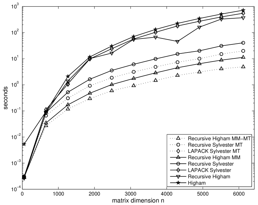
Figure 1: Running times on matrices with roughly balanced inertia.

The running times on matrices with roughly balanced inertia are shown in Figure 1. Our recursive algorithm is the fastest one, both with and without multithreaded BLAS. The next-best algorithm is the recursive Patlett-Sylvester algorithm. Like our recursive algorithm, it uses the BLAS extensively so it benefits from multithreading. Our recursive but arithmetic-efficient algorithm is fairly slow, because it does not use the BLAS. The slowest algorithms are the Parlett-Sylvester implementation that uses LAPACK for Schur reordering and for solving Sylvester equations and the element-by-element Parlett-Higham algorithm.

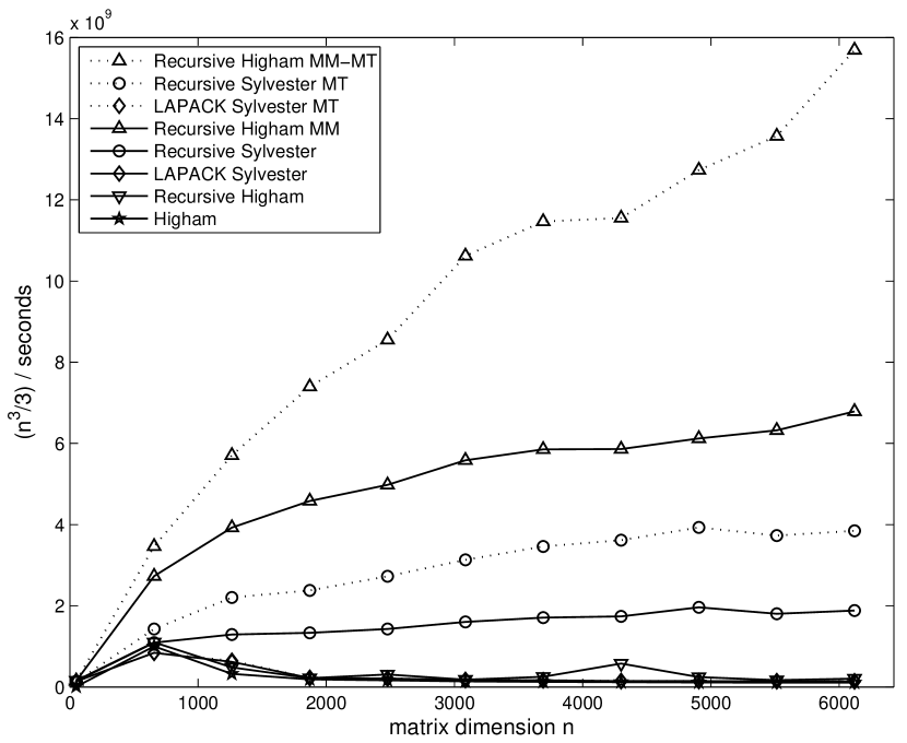
Figure 2: Normalized computational rates on matrices with roughly balanced inertia. The number $n^{3}/3$ is used for normalization because the number of arithmetic operations in Higham’s algorithm is between $n^{3}/3+o(n^{3})$ and $2n^{3}/3+o(n^{3})$; the number of operations in some of the other algorithms is different.

Figure 2 puts the same results in a somewhat more familiar quantitative context. By measuring performance in terms of normalized floating-point arithmetic rates, the performance of the algorithms can be directly compared to the performance of other algorithms (e.g., matrix multiplication) on the same computer. The rates are normalized relative to $n^{3}/3$ because the number of arithmetic operations in Higham’s algorithm is between $n^{3}/3+o(n^{3})$ and $2n^{3}/3+o(n^{3})$; other algorithms may perform more or less arithmetic.

Our recursive algorithm always performs $2n^{3}/3+o(n^{3})$; on large matrices it runs single threaded at a rate of about 12Gflop/s (not normalized). Multithreading on the quad-core computer speeds up the algorithm by more than a factor of 2 on large matrices (the speedup is around 2 rather than 4 because only matrix multiplications exploit more than one core). The recursive Parlett-Sylvester is about 3 times slower. The performance of the non-recursive algorithms (and of our recursive algorithm that does not use the BLAS) is quite dismal.

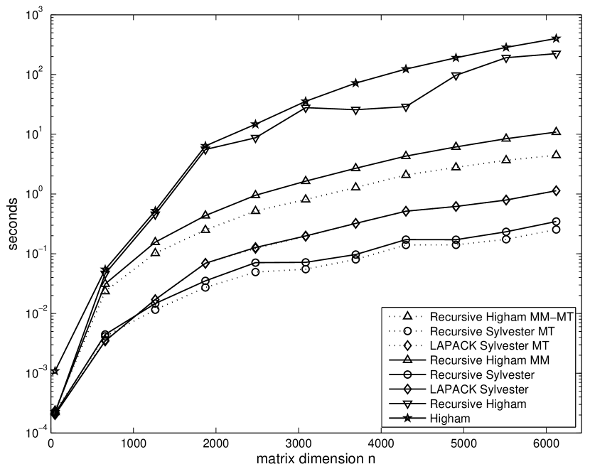
Figure 3: Running times on matrices with Exactly $3$ negative eigenvalues and $n-3$ positive eigenvalues.

When inertia is highly imbalanced, the picture changes. Figure 3 shows that Parlett-Sylvester algorithms are the fastest on such matrices. This makes sense, as they only perform $\Theta(n^{2})$ operations, not $\Theta(n^{3})$ like all the other algorithms. The differences are quite dramatic. The best single-threaded Parlett-Sylvester algorithm (Recursive Sylvester) runs in 0.35s on matrices of dimension 6120, whereas the fastest single-threaded recursive Higham algorithm takes 10.9s (more than 30 times slower). Figure 4 shows the corresponding normalized rates for completeness, but they are less interesting because the normalization factor is way off for the Parlett-Sylvester algorithms.

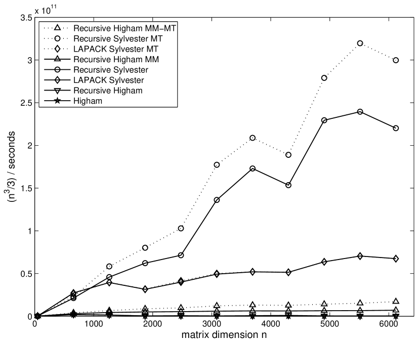
Figure 4: Normalized computational rates on matrices with Exactly $3$ negative eigenvalues and $n-3$ positive eigenvalues.

7 Conclusions

The reader may have been somewhat surprised by some aspects of this work. They also surprised us.

The first surprise is that arithmetic performance (number of operations) can differ so dramatically between the Parlett-Higham recurrence and its block variant that we refer to as Parlett-Sylvester. The striking efficiency of the Parlett-Sylvester approach on matrices with highly imbalanced inertia is the result of three contributing factors: (1) the performance of the Schur reordering algorithm depends strongly on the number of eigenvalue swaps required to order the matrix, (2) solving Sylverster equations on high-aspect ratio matrices is very inexpensive, and (3) computing the diagonal blocks in the Parlett-Sylvester algorithm for the sign function is trivial.

This finding implies that a production code for the sign function should choose between these two algorithms, ideally through an auto-tuning and/or performance-prediction framework, possibly based on inertia estimation.

Second, was the difficulty of expressing cleanly the recursive variant of the Higham-Parlett algorithm. We have tried a number of approaches based on conventional notational schemes and failed. We resorted to develop the somewhat complex notation that we present and use in Section 5; it may seem overly complex, but we found it impossible to present the algorithm without it.

The third (and relatively minor) surprise is the benefit of performing more arithmetic in order to use matrix-multiplication. The arithmetic-efficient variant of the recursive Parlett-Higham algorithm (Section 5.3) is slower in practice, although it is cache efficient. Rather than using existing matrix-multiplication routines (xGEMM), it uses a custom kernel with a condition in the next-to-inner loop. This demonstrated the performance penalty for trying to do less arithmetic in an algorithm using a conditional, thus making performance optimization difficult.

Acknowlegements

This research was supported in part by grants 863/15, 1878/14, and 1901/14 from the Israel Science Foundation (founded by the Israel Academy of Sciences and Humanities) , grant 3-10891 from the Ministry of Science and Technology, Israel. Research is also supported by the Einstein Foundation and the Minerva Foundation. This paper is supported by the Intel Collaborative Research Institute for Computational Intelligence (ICRI-CI). This research was supported by a grant from the United States-Israel Binational Science Foundation (BSF), Jerusalem, Israel. This work was supported by the HUJI Cyber Security Research Center in conjunction with the Israel National Cyber Bureau in the prime minister’s office.

References

- [1] Zhaojun Bai and James W. Demmel. On swapping diagonal blocks in real Schur form. Linear Algebra Appl., 186:73–95, 1993.
- [2] Grey Ballard, James Demmel, Olga Holtz, , and Oded Schwartz. Minimizing communication in linear algebra. SIAM Journal on Matrix Analysis and Applications, 32:866–901, 2011.
- [3] Philip I. Davies and Nicholas J. Higham. A Schur–Parlett algorithm for computing matrix functions. SIAM J. Matrix Anal. Appl., 25(2):464–485, 2003.
- [4] Gene Golub and Charles Van Loan. Matrix Computations. Johns Hopkins, 4th edition, 2013.
- [5] Nicholas J. Higham. Functions of Matrices: Theory and Algorithm. SIAM, 2008.
- [6] Dror Irony, Sivan Toledo, and Alexander Tiskin. Communication lower bounds for distributed-memory matrix multiplication. Journal of Parallel and Distributed Computing, 64:1017–1026, 2004.
- [7] Isak Jonsson and Bo Kågström. Recursive blocked algorithms for solving triangular systems: Part II: Two-sided and generalized Sylvester and Lyapunov matrix equations. ACM Transactions on Mathematical Software, 28(4):416–435, December 2002. The code is available at http://www8.cs.umu.se/~isak/recsy.
- [8] Daniel Kressner. Block algorithms for reordering standard and generalized schur forms. ACM Transactions on Mathematical Software, 32:521–532, 2006.
- [9] L. H. Loomis and H. Whitney. An inequality related to the isoperimetric inequality. Bulletin of the American Mathematical Society, 55:961–962, 1949.
- [10] Kwok Choi Ng. Contributions to the computation of the matrix exponential. Technical Report PAM-212, Center for Pure and Applied Mathematics, University of California, Berkeley, February 1984. PhD thesis.
- [11] Beresford N. Parlett. Computation of functions of triangular matrices. Memorandum ERL-M481, Electronics Research Laboratory, College of Engineering, University of California, Berkeley, November 1974.
- [12] Beresford N. Parlett. A recurrence among the elements of functions of triangular matrices. Linear Algebra Appl., 14:117–121, 1976.