Cosmological Tests with the FSRQ Gamma-ray Luminosity Function
Abstract
The extensive catalog of -ray selected flat-spectrum radio quasars (FSRQs) produced by Fermi during a four-year survey has generated considerable interest in determining their -ray luminosity function (GLF) and its evolution with cosmic time. In this paper, we introduce the novel idea of using this extensive database to test the differential volume expansion rate predicted by two specific models, the concordance CDM and cosmologies. For this purpose, we use two well-studied formulations of the GLF, one based on pure luminosity evolution (PLE) and the other on a luminosity-dependent density evolution (LDDE). Using a Kolmogorov-Smirnov test on one-parameter cumulative distributions (in luminosity, redshift, photon index and source count), we confirm the results of earlier works showing that these data somewhat favour LDDE over PLE; we show that this is the case for both CDM and . Regardless of which GLF one chooses, however, we also show that model selection tools very strongly favour over CDM. We suggest that such population studies, though featuring a strong evolution in redshift, may nonetheless be used as a valuable independent check of other model comparisons based solely on geometric considerations.
keywords:
quasars: general – cosmology: theory – large-scale structure of the universe1 Introduction
The discovery of quasars at redshifts (Fan et al., 2003; Jiang et al., 2007; Willott et al., 2007; Jiang et al., 2008; Willott et al., 2010a; Mortlock et al., 2011; Venemans et al., 2013; Banados et al., 2014; Wu et al., 2015) suggests that supermassive black holes emerged only Myr after the big bang, and only Myr beyond the formation of Population II and Population III stars (Melia, 2013a). Such large aggregates of matter constitute an enduring mystery in astronomy because these quasars could not have formed so quickly in CDM without an anomalously high accretion rate (Volonteri & Rees, 2006) and/or the creation of unusually massive seeds (Yoo & Miralda-Escudé, 2004); neither of these has actually ever been observed. For example, Willott et al. (2010b) have recently demonstrated that no known high- quasar accretes at more than times the Eddington rate (see Figure 5 in their paper; see also Melia 2014).
This paper will feature two specific cosmologies—the aforementioned CDM (the ‘standard,’ or concordance model) and another Friedmann-Robertson-Walker solution known as the Universe (Melia, 2007; Melia & Shevchuk, 2012; Melia, 2016). Our focus will be to explain the luminosity function of these quasars, particularly as they evolve towards lower redshifts. Part of the motivation for this comparative study is that, unlike CDM, the model does not suffer from the time compression problem alluded to above (Melia, 2013a). In this cosmology, cosmic reionization (starting with the creation of Population III stars) lasted from Myr to Gyr (), so black hole seeds formed (presumably during supernova explosions) shortly after reionization had begun, would have evolved into quasars by simply via the standard Eddington-limited accretion rate. The Universe has thus far passed all such tests based on a broad range of cosmological observations, but already, this consistency with the age-redshift relationship implied by the early evolution of supermassive black holes suggests that an optimization of the quasar luminosity function might serve as an additional powerful discriminator between these two competing expansion scenarios. The class of flat-spectrum radio quasars (FSRQs) is ideally suited for this purpose.
FSRQs are bright active galactic nuclei (AGNs) that belong to a subcategory of Blazars. These represent the most extreme class of AGNs, whose radiation towards Earth is dominated by the emission in a relativistic jet closely aligned with our line-of-sight. The discovery of -ray emission from these sources was an important confirmation of the prediction by Melia & Konigl (1989) that the particle dynamics in these jets ought to be associated with significant high-energy emission along small viewing angles with respect to the jet axis. It is still an open question exactly what powers the jet activity, but it is thought that the incipient energy is probably extracted from the black hole’s spin, and is perhaps also related to the accretion luminosity. Major mergers might have enhanced the black-hole growth rate and activity, which would have occurred more frequently in the early Universe. In this context, the Blazar evolution may be connected with the cosmic evolution of the black-hole spin distribution, jet activity and major merger events themselves, all of which may be studied via the luminosity function (LF) and its evolution with redshift.
Recently, the Fermi Gamma-ray Space Telescope has detected hundreds of blazars from low redshifts out to z = 3.1, thanks to its high sensitivity (Abdo et al., 2010a). Based on the previous analysis of the FSRQ -ray luminosity function (GLF), it is already clear that the GLF evolution is positive up to a redshift cut-off that depends on the luminosity (see, e.g., Padovani et al. 2007; Ajello et al. 2009; Ajello et al. 2012). But all previous work with this sample ignored a very important ingredient to this discussion—the impact on the GLF evolution with redshift from the assumed cosmological expansion itself. Our main goal in this paper is to carry out a comparative analysis of the standard CDM and models using the most up-to-date sample of 408 FSRQs detected by the Fermi-LAT over its four-year survey. We wish to examine the influence on the results due to the assumed background cosmology and, more importantly, we wish to demonstrate that the current sample of -ray emitting FSRQs is already large enough for us to carry out meaningful cosmological testing. Throughout this paper, we will be directly comparing the flat CDM cosmology with and km s-1 Mpc-1, based on the latest Planck results (Planck Collaboration, 2014), and the Universe, whose sole parameter—the Hubble constant—will for simplicity be assumed to have the same value as that in CDM. We will demonstrate that these data already emphatically favour over CDM, even without an optimization of for .
The outline of this paper is as follows. In § 2, we will summarize the observational data, specifically the 3FGL catalog (Acero et al., 2015), and describe how the -ray luminosity is determined for each specific model. § 3 will provide an account of the critical differences between these two cosmologies that directly impact the calculation of the GLF, and we discuss the currently preferred ansatz for this luminosity function based on the most recent analysis of these data in § 4. We present and discuss our results in § 5, and conclude in § 6.
2 Observational Data and Source Sample
The third Fermi Large Area Telescope source catalog (3FGL) provided by Acero et al. (2015) lists 3,303 sources detected by Fermi-LAT during its four years of operation. These data include the source location and its spectral properties. A subset of these is the third LAT AGN catalog (3LAC; Ackermann et al. 2015), containing 1,591 AGNs of various types located at high galactic latiude, i.e., . Most of the detected AGNs are blazars, which consist of 467 FSRQs, 632 BL Lacs, 460 blazar candidates of uncertain type (BCUs), and 32 non-blazar AGNs. Removing the entries in 3LAC for which the corresponding -ray sources were not associated with AGNs, had more than one counterpart or were flagged for other reasons in the analysis, Ackermann et al. (2015) reduced the AGN catalog to a ‘clean’ sample of 1,444 sources, including 414 FSRQs, 604 BL Lacs, 402 BCUs and 24 non-blazar AGNs. The energy flux distribution of all the Fermi sources may be seen in Figure 18 of Acero et al. (2015). The flux threshold in 3FGL is erg cm-2 s-1, lower than the value ( erg cm-2 s-1) in 2FGL and ( erg cm-2 s-1) in 1FGL. The sample above the 3FGL flux threshold is essentially complete (see Figure 18 of Acero et al. 2015). Note also that all of the FSRQs cataloged in 3FGL have measured redshifts. In this paper, we have chosen to use only the FSRQs from 3LAC, and not the BL Lacs, because of their greater redshift coverage and better sample completeness, both of which strengthen our statistical analysis.
Our sample is therefore comprised of the 414 FSRQs detected by Fermi with a test statistic (TS) and latitude . Their -ray fluxes and photon indices in the energy range 0.1 GeV - 100 GeV are obtained from 3FGL111URL: and their redshifts are from Table 7 of Ackermann et al. (2015).222URL: We calculate the -ray luminosity of an FSRQ using the expression:
| (1) |
where is the luminosity distance at redshift and is the correction for the observed fluxes using . The corresponding photon flux (in units of photons cm-2 s-1) in the 0.1 GeV - 100 GeV energy band used in this paper is readily obtained from the following expressions (see, e.g., Ghisellini et al. 2009, Singal et al. 2014):
| (4) |
where erg (corresponding to 0.1 GeV) is the lower energy limit.
|

|
Clearly, a determination of requires the assumption of a particular cosmological model. A detailed description of the differences between the two models we are considering here, the concordance CDM cosmology and the Universe, may be found in Melia (2012a, b, 2013a, 2013b). The quantity most relevant to the analysis in this paper is the luminosity distance , which in CDM is given as
| (5) | |||||
where is the speed of light and is the Hubble constant at the present time. In this equation, and are, respectively, the energy density of matter and dark energy written in terms of today’s critical density (), and is the spatial curvature of the Universe, appearing as a term proportional to the spatial curvature constant k in the Friedmann equation. Also, is when and when . For a flat universe with , Equation (5) simplifies to the form times the integral. In the Universe, the luminosity distance is given by the much simpler expression
| (6) |
where is the gravitational horizon (equal to the Hubble radius) at the present time.
The luminosities in these two models are simply related according to the expression
| (7) |
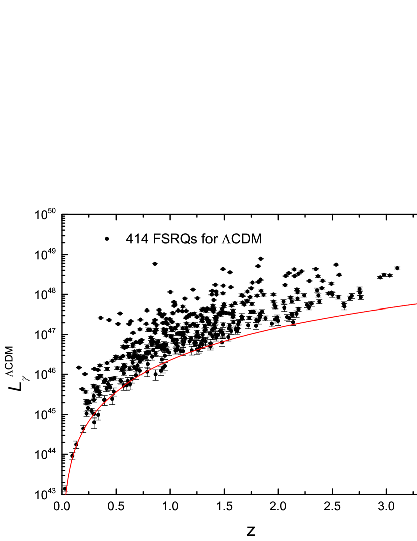
Figure 1 shows the resulting luminosity-redshift distribution for both CDM (left panel) and (right panel). In this figure, the solid curves are calculated using Equation (1) for the threshold flux erg cm-2 s-1, and a fixed photon index , which is the mean of the distribution from 3LAC (Ackermann et al., 2015). For a given observed flux, , the inferred luminosity depends on the assumed cosmology through the model-dependent luminosity distance, , as indicated in Equation (5). The data points in figure 1 are therefore slightly different for the two models being compared here. However, since we are assuming the concordance model with Planck parameters (see below), it turns out that the ratio is very close to over the redshift range . One may see this in figure 3 of Melia (2015), which plots this ratio for several values of the matter density . For the Planck matter density , is just a few percent bigger than over the entire redshift range considered in this paper.
3 Model Comparison
Given a fixed background cosmology, we constrain the model parameters of the FSRQs GLF (see § 4) using the method of maximum likelihood evaluation (see, e.g., Chiang & Mukherjee 1998; Ajello et al. 2009; Norumoto et al. 2006; Abdo et al. 2010b; Zeng et al. 2014). The likelihood function is defined by the expression
| (8) |
where is the space density of FSRQs, which generally depends on the luminosity function, ; the intrinsic distribution of photon indices with a Gaussian dependence, , where and are the Gaussian mean and dispersion, respectively; and the comoving volume element per unit redshift and unit solid angle, . This space density may be expressed as
| (9) | |||||
In Equation (6), the quantity is the expected number of FSRQ -ray detections,
| (10) | |||||
Based on the properties of the -ray emitting FSRQ sample, we take , , , , erg s-1, and erg s-1. The quantity is the detection efficiency, and represents the probability of detecting a FSRQ with the photon flux and photon index (e.g., Atwood et al. 2009; Abdo et al. 2010c; Ajello et al. 2012; Zeng et al. 2013; DiMauro et al. 2014a, 2014b), where is strongly dependent on the photon index (obtained from Equations 1 and 2), and is also a function of the luminosity and redshift . To estimate , we use the method provided by Di Mauro et al. (2014a). The efficiency at a photon flux and photon index may be estimated as
| (11) |
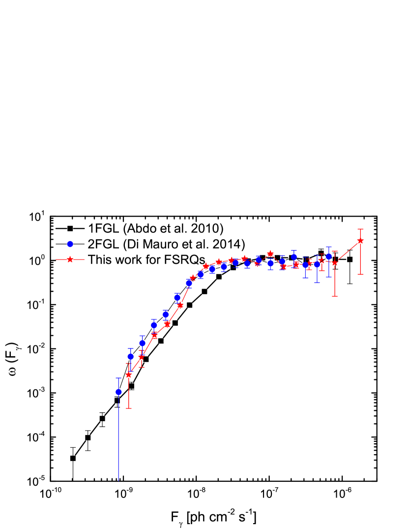
where is the solid angle associated with , is the incompleteness of the sample representing the ratio of unassociated sources to the total number of sources, and is the number of selected sources. The integrated values of and are, respectively, the intrinsic flux and index distributions of the sources. Note that the effect of the photon index on the detection efficiency is fully accounted for in our method, the details of which are discussed in the Appendix of Di Mauro et al. (2014a). Here we assume that the intrinsic flux distributions in the low flux band of FSRQs and blazars have the same power-law index, because the distribution log-log of FSRQs is flatter than that of blazars at low fluxes (see Figure 14 of Abdo et al. 2010c). Figure. 11 shows the efficiency for this sample of FSRQs evaluated using Eq. 11, in the region , compared with the 1FGL (Abdo et al., 2010c) and 2FGL (Di Mauro et al., 2014a) samples. This comparison shows that this method of evaluation is a simplified and effective way to find the efficiency, though the correct method would include a simulation and an estimate of the number of detected sources versus the number of simulated objects in different flux bins (Abdo et al., 2010c; Ackermann et al., 2016).
While maximization of the likelihood function is an appropriate and reliable method for optimizing the parameters of a given model, to determine statistically which of the models is actually preferred by the data it is now common in cosmology to use several model selection tools (see, e.g., Melia & Maier 2013, and references cited therein). These include the Akaike Information Criterion, , where is the number of free parameters (Liddle 2007); the Kullback Information Criterion, (Cavanaugh 2004); and the Bayes Information Criterion, , where is the number of data points (Schwarz 1978). A more quantitative ranking of models can be computed as follows. When using the AIC, with characterizing model , the unnormalized confidence in is given by the Akaike weight exp. The relative probability that is statistically preferred is
| (12) |
The difference determines the extent to which is favoured over . For Kullback and Bayes, the likelihoods are defined analogously. In using these model selection tools, the outcome (and analogously for KIC and BIC) is judged to represent ‘positive’ evidence that model 1 is to be preferred over model 2 if . If , the evidence favouring model 1 is moderate, and it is very strong when .
In this paper, we have chosen to compare two specific models: the concordance CDM cosmology, with Planck-measured prior values for all its parameters, and the Universe, whose sole parameter—the Hubble constant —is, for simplicity, assumed to have the same value as that in CDM. The total number of free parameters in this study is therefore limited in both cases to the formulation of the -ray luminosity function (GLF) (see § 4), which is common to both models. In other words, the model selection statistic we will be using, i.e., (for AIC, KIC, or BIC, as the case may be), depends solely on the quantity and in fact, for this reason, all three of these information criteria share the same values of . As it turns out, represents the distribution. Transforming to the standard expression, we may therefore write
| (13) |
For each model, we optimize the GLF parameters using the Markov Chain Monte Carlo (MCMC) technology, which is widely applied to give multidimensional parameter constraints from observational data. In practice, this means we will find the parameter values that minimize , which yields the best-fit parameters and their associated errors. We have adapted the MCMC code from COSRAYMC (Liu et al., 2007), which itself was adapted from the COSMOMC package (Lewis & Bridle, 2002). Additional details about the MCMC method may be found in Gamerman (1997) and Mackay (2003). We remark here that this way of posing the maximum likelihood problem is different from that chosen by Ajello et al. (2009, 2012, 2014) but, as pointed out in Ajello et al. (2009), who tested these various approaches, one gets exactly the same results using these different formulations, so there is no preference for one over the other, except in terms of convenience.
One of the principal differences between the two models affecting the value of is the space density of FSRQs due to its dependence on the luminosity distance . The comoving differential volume is given as
| (14) |
where is the comoving distance. For flat CDM and we have, respectively,
| (15) |
and
| (16) |
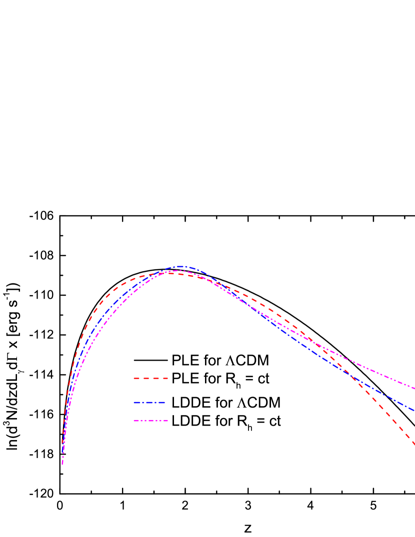
For illustration, we show in Figure 2 the space density (Equation 7) as a function of redshift , using the two formulations of the GLF described below, i.e., for pure luminosity evolution (PLE) and for luminosity-dependent density evolution (LDDE). The choice of parameters in this example is based on the discussion in § 5.
4 The Gamma-ray Luminosity Function
The so-called pure luminosity evolution (PLE) formulation for the GLF is motivated by the observed space density of radio-quiet AGNs, peaking at intermediate redshifts that correlate with source luminosity (see, e.g., Ueda et al. 2003; Hasinger et al. 2005). This peak may correspond to the combined effect of black-hole growth and the falloff in fueling activity. The conventional formulation for the space density of this GLF (see, e.g., Ajello et al. 2012) has the form
| (17) | |||||
where is the evolution factor correlated with source luminosity, is a normalization factor, is the evolving break luminosity, is the faint-end slope index, is the bright-end slope index, and and represent the redshift evolution. Including the additional parameters and characterizing the (Gaussian) photon index distribution (see discussion following Equation 6) then results in a total of 8 parameters that need to be optimized in our PLE analysis.
However, while the PLE GLF generally provides a good fit to the observed redshift and luminosity distributions, it is a very poor representation of the observed - (Ajello et al. 2012). Closer scrutiny of the values of and in in different redshift bins suggests that there is a significant shift in the redshift peak, with the low- and high-luminosity samples peaking at and , respectively.
Since the simple PLE GLF may not be a completely adequate fit to the Fermi data, and since the redshift peak apparently evolves with luminosity, it is also beneficial to consider a GLF with luminosity-dependent density evolution (LDDE; see Ueda et al. 2003; Ajello et al. 2012). In this formulation, the GLF evolution is decided by a redshift cut-off that depends on luminosity. The space density for this GLF is given by the expression
| (18) | |||||
with
| (19) |
where is a normalization factor, is the evolving break luminosity, and are the faint-end slope indeces, and are the bright-end slope indeces, is the redshift peak with luminosity ergs s-1, and is the power-law index of the redshift-peak evolution.
Previous studies based solely on the concordance CDM model (see, e.g., Ajello et al. 2012) have shown that the LDDE provides a good fit to the LAT data and can reproduce the observed distribution quite well. The log-likelihood ratio test strongly favours it over PLE. In this paper, we will use both formulations of the GLF, just to be sure that we are not biasing our results prematurely with an ansatz for that is too specific. As it turns out, both the PLE and LDDE formulations give completely consistent results when it comes to model selection. We will therefore conclude that the results of our model comparison using the -ray emitting FSRQs is not at all dependent on assumptions concerning the form of the GLF.
| PLE | log | log | |||||||||
| CDM | 67.3 | 0.315 | 89106 | ||||||||
| 67.3 | 88962 | ||||||||||
| KS Test | |||||||||||
| CDM | 98.4% | 67.5 % | 72.9 % | ||||||||
| 98.6% | 73.4 % | 74.9 % | |||||||||
| a In units of km s-1 Mpc-1 | |||||||||||
| b In units of Mpc-3 erg-1 s | |||||||||||
5 Results and Discussion
5.1 Pure Luminosity Evolution
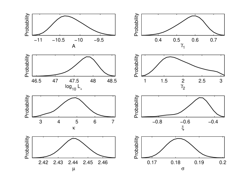
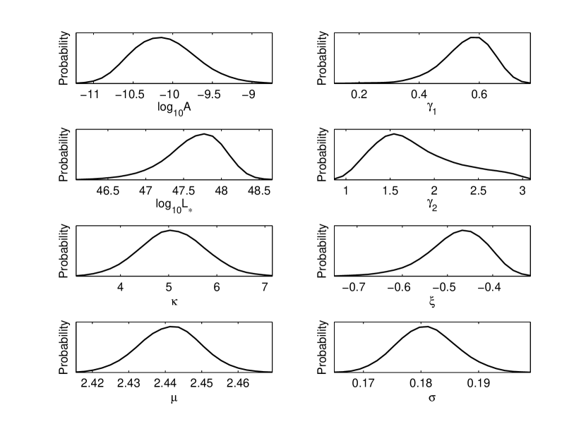
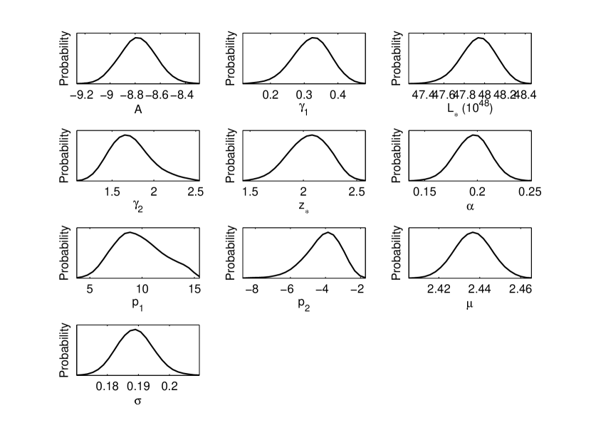
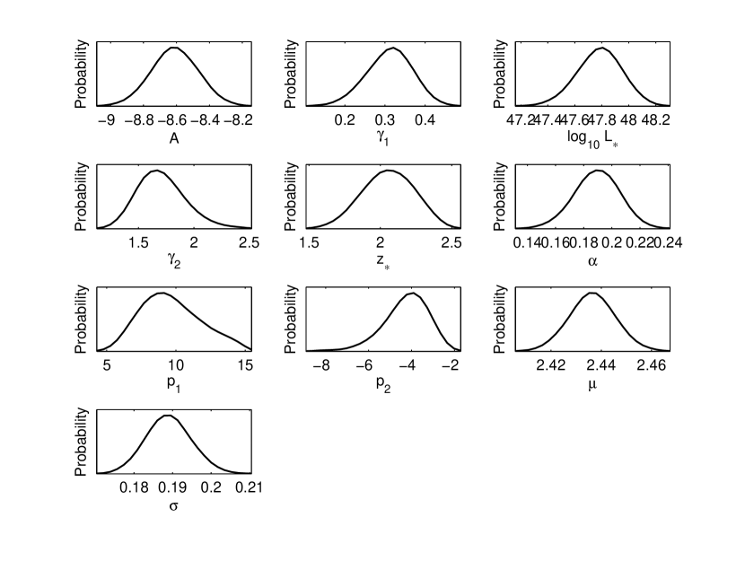
We begin with the PLE assumption and optimize the GLF parameters by maximizing the likelihood function using the MCMC method. The best-fit parameters and one-dimensional (1D) probability distributions are shown in Figure 3 for CDM and Figure 4 for . The mean-fit parameter values and their 1 confidence levels are listed in Table 1.
Ajello et al. (2012) examined whether the PLE GLF could adequately account for the Fermi data, though strictly only for the CDM cosmology, and concluded that it was not a good representation of the - distribution. To see whether this is still true for our sample, and also to test whether this defiiciency is also present for the Universe, we apply the Kolmogorov-Smirnov (KS) test for the predicted one-parameter cumulative distributions using the measured populations as individual functions of redshift, luminosity and photon index. The theoretical one-parameter distributions are calculated as follows:
| (20) | |||||
| (21) | |||||
| (22) | |||||
In addition, the source count distribution is given by the expression
| (23) | |||||
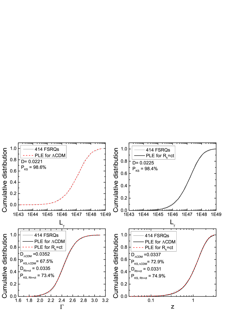
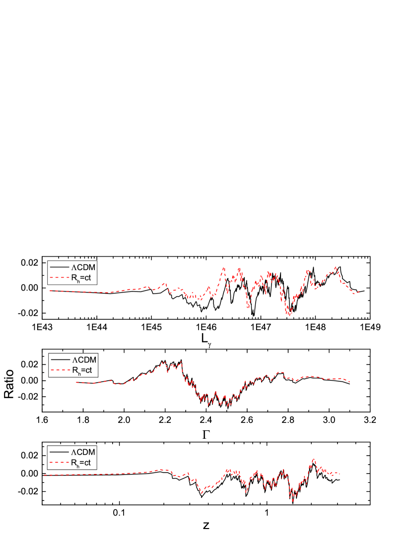
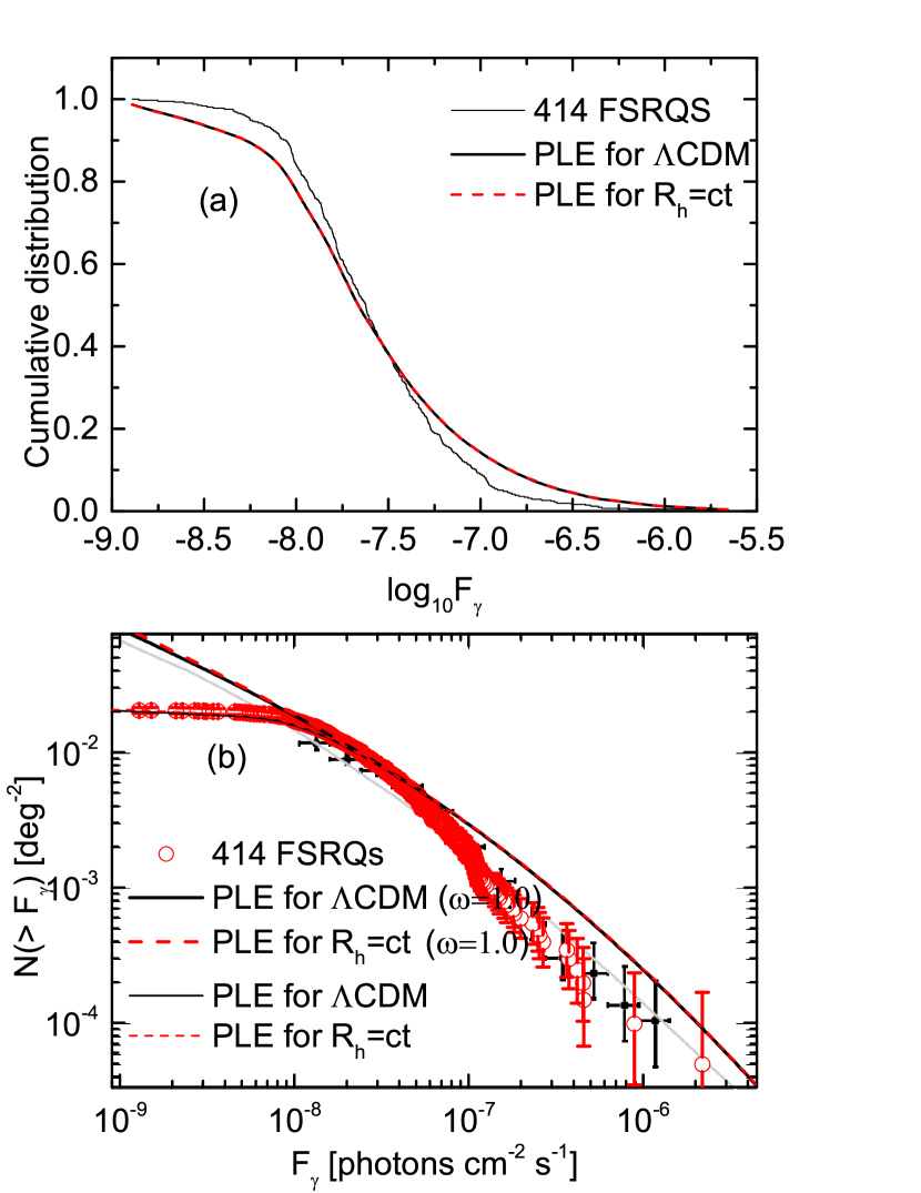
where is the luminosity of a source at redshift with photon index , having a flux . The corresponding curves, together with the binned data with which they are compared, are shown in Figures 5 and 9 for both CDM and .
At least visually, the predicted cumulative distributions appear to match the data quite well, aside from the source count distribution. Indeed, the PLE GLF passes the KS test in three cumulative distributions (luminosity, redshift, photon index) for both cosmologies, though only at a modest level of confidence in the case of . The Universe does better than the concordance CDM model for all the distributions. As we shall see shortly, the results of our KS comparison between the cumulative distributions for PLE and LDDE are somewhat mixed. Certainly in the case of , the LDDE GLF passes the KS test with a significantly higher level of confidence, where it reaches in the case of , compared to only for PLE. However, the KS test results for the cumulative distributions in are very similar between PLE and LDDE. Note that the left panels in Figure 9 show that the predicted distributions are a very poor representation of the observed log-log. Based solely on the cumulative redshift distribution, together with the relatively poor source-count distribution, we do confirm the result in Ajello et al. (2012), that the LDDE GLF appears to be a better representation of the Fermi data than the PLE GLF.
5.2 Luminosity-Dependent Density Evolution
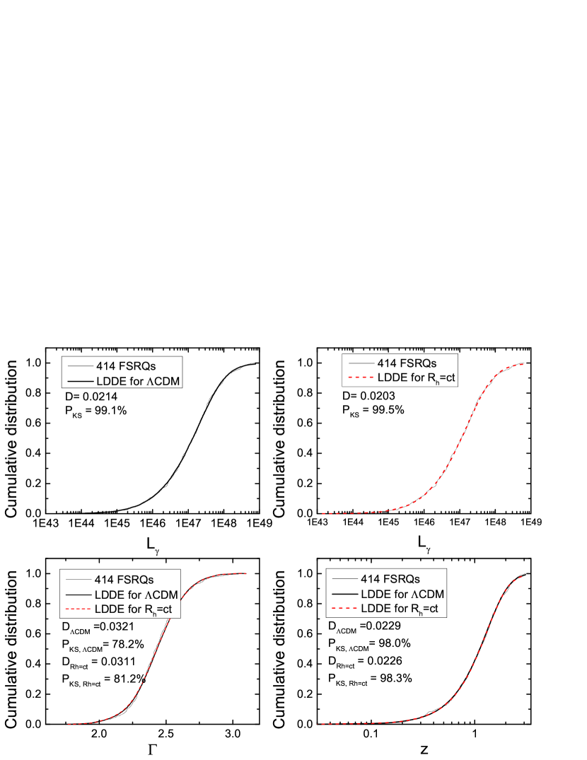
We next optimize the ten parameters of the LDDE GLF, given in Equation (16), using the MCMC method to maximize the likelihood function for the same sample of 414 FSRQs that we used for PLE. The 1D probability distributions of these parameters are shown in Figure 6 for CDM and Figure 7 for . Their mean-fit values and 1 confidence levels are listed in Table 2. As before, and specifically to examine which GLF is a better match to the data, we carry out the same Kolmogorov-Smirnov test as for PLE, and compare the predicted one-parameter cumulative distributions with the data in Figure 8. The favorable visual impression one gets is confirmed by the confidence levels of the matches, which are quoted in Table 2.
| LDDE | a | log | log | ||||||||||
| CDM | 0.315 | 89047 | |||||||||||
| 0.673 | 88903 | ||||||||||||
| KS Test | |||||||||||||
| CDM | 99.1% | 78.2 % | 98.0 % | ||||||||||
| 99.5% | 81.2 % | 98.3 % | |||||||||||
| a In units of km s-1 Mpc-1 | |||||||||||||
| b In units of Mpc-3 erg-1 s | |||||||||||||
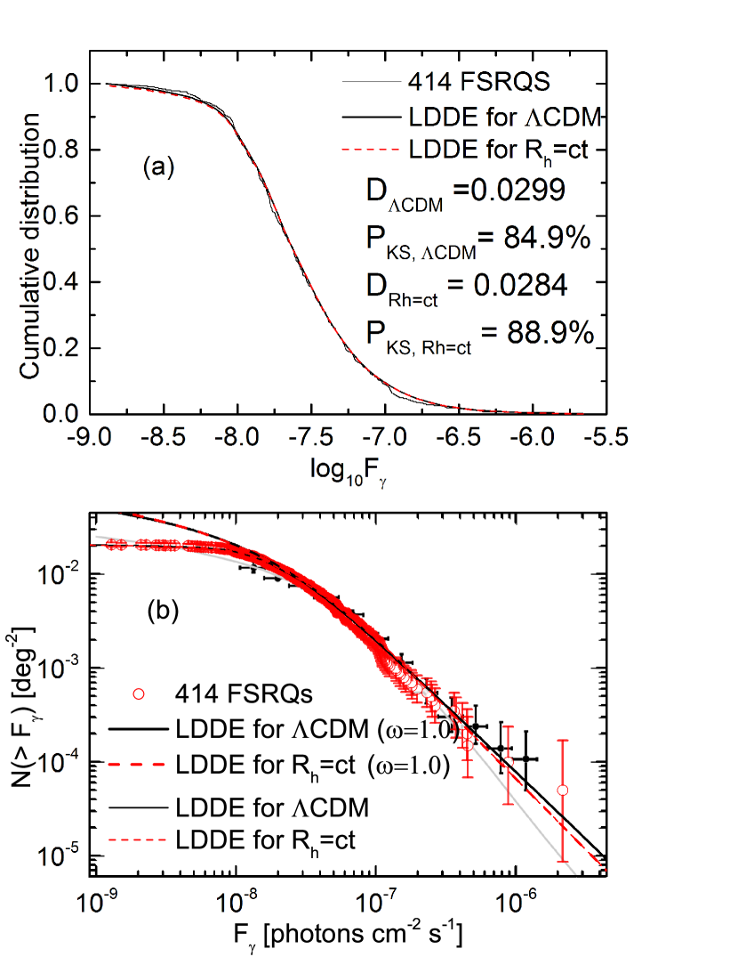
The cosmology does at least as well as CDM, and usually better, in all the KS tests using the various one-parameter cumulative FSRQ distributions. In both models, the predicted source count distribution is a better match to the data for LDDE than for PLE (the right-hand panels of Figure 9), supporting the conclusion drawn earlier by Ajello et al. (2012) that LDDE is favoured over PLE by the measured - relation.
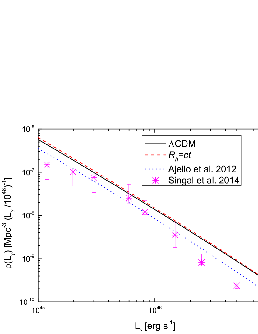
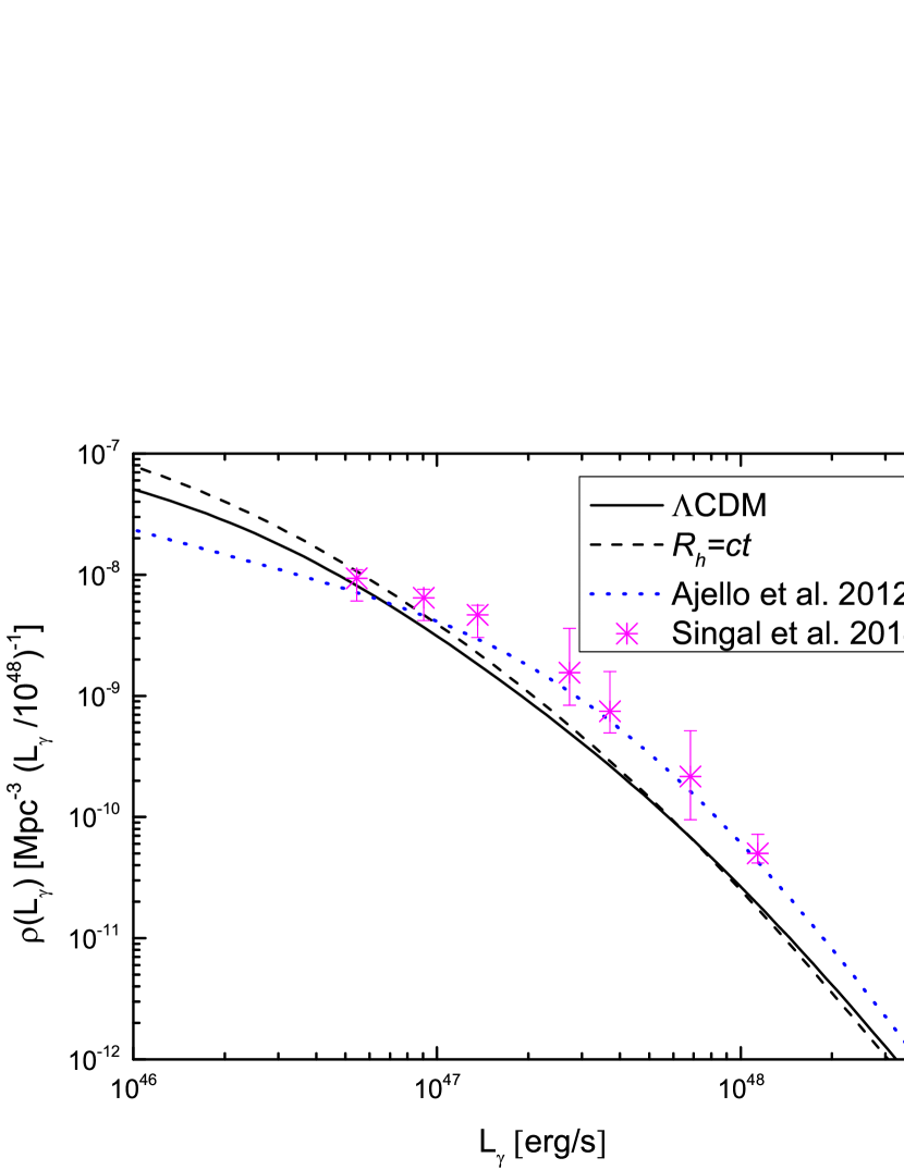
To complete our discussion, we also summarize here a comparison of our results with others reported in the literature. Since LDDE appears to be strongly favoured by the data over PLE, we will focus our attention on this particular GLF. Figure 10 compares the differential local (z=0) and z=1 GLFs with those reported by Ajello et al. (2012) and Singal (2014). Ajello et al. (2012) analyzed the LF by using the sample comprised of 186 FSRQs detected by Fermi with , and photons cm-2 s-1. The results of Singal (2014) were obtained by analysing the sample of 184 FSRQs with , reported by Shaw et al. (2012). We can see that our distributions have a normalization approximately two times larger than theirs. This is merely a reflection of the fact that our sample (414) is about two times bigger than theirs (186 and 184); other than this obvious difference, our results for the local universe are virtually identical to theirs. The right-hand plot in Figure 10 shows some slight differences in the determination of the GLF at , possibly due to the different redshift distributions of the various samples used for the optimization of the model parameters or the incompleteness of the earlier samples. In this regard, we note from the bottom panels of Figure 9 that the observed data of our sample are concordant with those of Ajello et al. (2012) at high fluxes, but they clearly differ in the low flux region. This would confirm the fact that our results should be the same at low redshifts, but differ with Ajello et al. (2012) at high redshifts, as is evident in Figure 10.
|
|
5.3 Model Comparisons
We now turn to the main goal of our analysis, which is to directly compare these two cosmologies, for which we must use the model selection tools discussed in § 3 above. Starting with the PLE GLF (§ 5.1), the values of (from which is calculated) are shown in Table 1. Our optimization procedure shows that (for this assumed PLE luminosity function) is , well into the ‘very strong’ category. At least for the PLE GLF, the size of our -ray emitting FSRQ sample is already large enough for this statistical assessment to overwhelmingly favour over the concordance CDM model.
As we have seen, the LDDE GLF is a significantly better match to the data than PLE. Here too, the model selection tools very strongly favour over CDM. In the case of LDDE, , which again is well into the ‘very strong’ category. The choice of GLF does not appear to have much influence in deciding which of these two cosmologies is favoured by the Fermi FSRQ data. The sample is already large enough for the observations to strongly prefer the differential volume dependence on predicted by over that in CDM.
6 Conclusions
The extensive, high-quality sample of -ray emitting FSRQs observed by Fermi has generated considerable interest in identifying the -ray luminosity function and its evolution with cosmic time. The number density of such objects has changed considerably during the expansion of the Universe, growing dramatically up to redshift and declining thereafter. Aside from the obvious benefits one may derive from better understanding this evolution as it relates to supermassive black-hole growth and its connection to the halos of host galaxies, its strong dependence on redshift all the way out to offers the alluring possibility of using it to test different cosmological models.
In this paper, we have introduced this concept by directly comparing two specific expansion scenarios, chiefly to examine the viability of the method. To do so, we have opted to use prior values for the model parameters themselves, and instead focus on the optimization of the parameters characterizing the chosen ansatz for the luminosity function. In doing so, one may question whether the choice of GLF unduly biases the fit for one model or the other. This is a legitimate concern, and considerable work still needs to be carried out to ensure that one is not simply customizing the GLF for each background cosmology.
For this reason, we have opted in this paper to use two different forms of the GLF, one for pure luminosity evolution and the second for a luminosity-dependent density evolution, even though earlier work had already established a preference by the data for the latter over the former. We have found that selecting either of these GLFs has no influence at all on the outcome of model comparison tools. In both cases, information criteria, such as the AIC, KIC, and BIC, show quite conclusively that the evolution of the GLF for FSRQs very strongly favours over the concordance CDM model.
Cosmic evolution is now studied using a diversity of observational data, including high- quasars (Melia 2013a, 2014), Gamma-ray bursts (Wei et al. 2013), the use of cosmic chronometers (Melia & Maier 2013; Melia & McClintock 2015), type Ia supernovae (Wei et al. 2015) and, most recently, an application of the Alcock-Paczyński test using model-independent Baryon Acoustic Oscillation (BAO) data (Font-Ribera et al., 2014; Delubac et al., 2015; Melia & López-Corredoira, 2015), among others. The BAO measurements are particularly noteworthy because, with their accuracy, they now rule out the standard model in favour of at better than the C.L.
|
|
In this paper, we have provided a compelling confirmation of these other results by demonstrating that population studies, though featuring a strong evolution in redshift, may also be used to independently check the outcome of model comparisons based purely on geometric considerations. We emphasize, however, that much work still needs to be done to properly identify how to best characterize the number density function for this type of analysis. This would be critically important in cases, unlike CDM and , where cosmological models are so different that an appropriate common ansatz may be difficult to find.
Acknowledgements
We thank the referee, Mattia Di Mauro, for a careful reading of our manuscript, and for thoughtful comments that have led to an improvemed presentation, including several clarifying descriptions of the results. We acknowledge the use of COSRAYMC (Liu et al. 2012) adapted from the COSMOMC package (Lewis & Bridle 2002). FM is grateful to Amherst College for its support through a John Woodruff Simpson Lectureship, and to Purple Mountain Observatory in Nanjing, China, for its hospitality while part of this work was being carried out. LZ acknowledges partial funding support by the National Natural Science Foundation of China (NSFC) under grant No. 11433004. This work was partially supported by grant 2012T1J0011 from The Chinese Academy of Sciences Visiting Professorships for Senior International Scientists, and grant GDJ20120491013 from the Chinese State Administration of Foreign Experts Affairs. This work is also supported by the Key Laboratory of Particle Astrophysics of Yunnan Province (Grant 2015DG035). This work is also partially supported by the Strategic Priority Research Program, the Emergence of Cosmological Structures, of the Chinese Academy of Sciences, Grant No. XDB09000000, and the NSFC grants 11173064, 11233001, and 11233008.
References
- Author (2012) Author A. N., 2013, Journal of Improbable Astronomy, 1, 1
- Others (2013) Others S., 2012, Journal of Interesting Stuff, 17, 198
- Abdo et al. (2010a) Abdo, A. A., Ackermann, M., Ajello, M., et al. 2010a, ApJ, 715, 429
- Abdo et al. (2010b) Abdo, A. A., et al. 2010b, Phys. Rev. Lett., 104, 101101-7.
- Abdo et al. (2010c) Abdo, A. A., et al. 2010c, ApJ, 720, 435
- Acero et al. (2015) Acero. F., et al. 2015 (ArXiv:1501,02003)
- Ackermann et al. (2015) Ackermann. M., et al. 2015 (ArXiv:1501,06054)
- Ackermann et al. (2016) Ackermann. M., et al. 2016, Phys. Rev. Lett. 116, 151105
- Ajello et al. (2009) Ajello, M., Costamante, L., Sambruna, R. M., et al. 2009, ApJ, 699, 603
- Ajello et al. (2012) Ajello, M., Shaw, M. S., Romani, R. W., et al. 2012, ApJ, 751, 108
- Ajello et al. (2014) Ajello, M., Romani, R. W., Gasparrini, D., et al. 2014, ApJ, 780,73
- Atwood et al. (2009) Atwood W. B. et al., 2009, ApJ, 697, 1071
- Banados et al. (2014) Banados, E. et al. 2014, AJ, 148, 14
- Cavanaugh (2004) Cavanaugh, J. E. 2004, Aust. N. Z. J. Stat., 46, 257
- Chiang & Mukherjee (1998) Chiang, J., & Mukherjee, R. ApJ, 1998, 496, 752-760.
- Delubac et al. (2015) Delubac, T. et al. 2015, A&A, submitted, arXiv:1404.1801
- Di Mauro et al. (2014a) Di Mauro, M. Calore, F. et al. 2014a, ApJ, 780,161
- Di Mauro et al. (2014b) Di Mauro, M. Calore, F. et al. 2014b, ApJ, 786,129
- Fan et al. (2003) Fan, X. et al. 2003, AJ, 125, 1649
- Font-Ribera et al. (2014) Font-Ribera, A. et al. 2014, JCAP, 5, id. 27
- Gamerman (1997) Gamerman, D. 1997, Markov Chain Monte Carlo: Stochastic Simulation for Bayesian Inference. Chapman and Hall, London
- Ghisellini (2009) Ghisellini G., Maraschi L., Tavecchio F., 2009, MNRAS, 396, L105
- Hasinger et al. (2005) Hasinger, G., Miyaji, T. & Schmidt, M. 2005, A&A, 441, 417
- Jiang et al. (2007) Jiang, L. et al. 2007, AJ, 134, 1150
- Jiang et al. (2008) Jiang, L. et al. 2008, AJ, 135, 1057
- Lewis & Bridle (2002) Lewis, A., & Bridle, S. 2002, Phys. Rev. D, 66, 103511
- Liddle (2007) Liddle, A. R. 2007, MNRAS, 377, L74
- Liu et al. (2007) Liu, J., Yuan, Q., Bi, X. J., Li, H., & Zhang, X. M. 2012, Phys. Rev. D, 85, d3507
- Mackay (2003) Mackay D. J. C., 2003, Information Theory, Inference and Learning Algorithms. Cambridge Univ. Press, Cambridge
- Melia (2007) Melia, F. 2007, MNRAS, 382, 1917
- Melia (2012a) Melia, F. 2012a, AJ, 144, 110
- Melia (2012b) Melia, F. 2012b, arXiv:1205.2713
- Melia (2013a) Melia, F., 2013a, ApJ, 764, 72
- Melia (2013b) Melia, F. 2013b, A&A, 553, 76
- Melia (2014) Melia, F. 2014. JCAP, 01, id. 027
- Melia (2015) Melia, F. 205, Astroph. Sp. Sci., 356, 393
- Melia (2016) Melia, F. 2016, Frontiers of Physics, 11, 119801
- Melia & Konigl (1989) Melia, F. & Konigl, A. 1989, ApJ, 340, 162
- Melia & López-Corredoira (2015) Melia, F. & López-Corredoira, M. 2015, ApJ, submitted, arXiv:1503.05052
- Melia & Maier (2013) Melia, F. & Maier, R. S. 2013, MNRAS, 432, 2669
- Melia & McClintock (2015) Melia, F. & McClintock, T. M. 2015, AJ, 150, id.119
- Melia & Shevchuk (2012) Melia, F. and Shevchuk, A.S.H. 2012, MNRAS, 419, 257
- Mortlock et al. (2011) Mortlock, D. J. et al. 2011, Nature, 474, 616
- Narumoto & Totani (2006) Narumoto, T., & Totani, T. ApJ, 2006, 643, 81-91.
- Volonteri & Rees (2006) Volonteri M., Rees M. J., 2006, ApJ, 650, 669
- Padovani et al. (2007) Padovani, P., Giommi, P., Landt, H., & Perlman, E. S. 2007, ApJ, 662, 182
- Planck Collaboration (2014) Planck Collaboration, Ade, P. A. R., Aghanim, N., et al. 2014, A&A, 571, A16
- Schwarz (1978) Schwarz, G. 1978, Ann. Statist., 6, 461
- Shaw (2012) Shaw, M. S., Romani, R. W., Cotter, G., et al. 2012, ApJ, 748, 49
- Singal (2014) Singal, J. Ko, A. & Petrosian, V. 2014, ApJ, 786, 109
- Ueda et al. (2003) Ueda, Y., Akiyama, M., Ohta, K. & Miyaji, T. 2003, ApJ, 598, 886
- Venemans et al. (2013) Venemans, E. P. et al. 2013, ApJ, 779, 24
- Wei et al. (2013) Wei, J.-J., Wu, X.-F. & Melia, F. 2013, ApJ, 772, 43
- Wei et al. (2015) Wei, J.-J., Wu, X.-F., Melia, F. & Maier, R. S. 2015, AJ, 149, 102
- Willott et al. (2007) Willott, C. J. et al. 2007, AJ, 134, 2435
- Willott et al. (2010a) Willott, C. J. et al. 2010a, AJ, 139, 906
- Willott et al. (2010b) Willott, C. J. et al. 2010b, AJ, 140, 546
- Wu et al. (2015) Wu, X.-B. et al. 2015, Nature, 518, 512
- Yoo & Miralda-Escudé (2004) Yoo, J. and Miralda-Escudé, J. 2004, ApJL, 614, L25
- Zeng et al. (2014) Zeng, H., Yan, D. and Zhang, Li 2014, MNRAS, 441, 1760