Abstract

We study the 2HDM contribution to the muon anomalous magnetic moment $a_{\mu}$ and present the complete two-loop result, particularly for the bosonic contribution. We focus on the Aligned 2HDM, which has general Yukawa couplings and contains the type I, II, X, Y models as special cases. The result is expressed with physical parameters: three Higgs boson masses, Yukawa couplings, two mixing angles, and one quartic potential parameter. We show that the result can be split into several parts, each of which has a simple parameter dependence, and we document their general behavior. Taking into account constraints on parameters, we find that the full 2HDM contribution to $a_{\mu}$ can accommodate the current experimental value, and the complete two-loop bosonic contribution can amount to $(2\cdots 4)\times 10^{-10}$, more than the future experimental uncertainty.

1 Introduction

The measured properties of the Higgs boson discovered at the LHC [1, 2] are compatible with the Standard Model (SM) [3]. However, there is room for alternative explanations of the Higgs boson and electroweak symmetry breaking in models with extended Higgs sectors. The two-Higgs doublet model (2HDM) is a particularly interesting framework to be studied. In a large part of its parameter space it is compatible with experimental data, it can originate from more fundamental theories like the MSSM, and it predicts a multitude of observable effects by which it can be studied and constrained.

Here we focus on the muon anomalous magnetic moment $a_{\mu}=(g_{\mu}-2)/2$ in the 2HDM. This is one of the most useful precision observables to provide complementary, non-collider constraints of extensions of the SM [4, 5, 6]. After significant recent progress on all aspects of the SM prediction, there is a stable $3$–$4\,$$\sigma$ deviation between the SM prediction and the Brookhaven measurement [7],

$$a_{\mu}^{\text{Exp$-$SM}} =\begin{cases}(28.7\pm 8.0)\times 10^{-10}\mbox{\cite[cite]{[\@@bibref{}{Davier}{}{}]}},\\ (26.1\pm 8.0)\times 10^{-10}\mbox{\cite[cite]{[\@@bibref{}{HMNT}{}{}]}},\end{cases}$$ (1)

using the indicated references for the hadronic vacuum polarization contributions.

Several recent studies [28, 29, 30, 31, 32, 33, 34] have shown that the 2HDM has viable parameter regions in which this (or at least most of this) deviation is explained. The existing studies evaluate $a_{\mu}$ in the 2HDM using one-loop and particular two-loop diagrams, so-called Barr-Zee diagrams. Such Barr-Zee diagrams were first considered in Ref. [35] and for $a_{\mu}$ in the 2HDM in Refs. [36, 37, 38, 39]; the most complete calculation is presented in Ref. [30]. Here we present and document the full two-loop calculation of $a_{\mu}$ in the 2HDM, including Barr-Zee and non-Barr-Zee diagrams.

Our calculation is motivated in two ways. Firstly, the 2HDM one-loop contributions are suppressed by two additional powers of the small muon Yukawa coupling. Thus the one-loop contributions are parametrically smaller than the two-loop contributions. In this sense our calculation completes the leading-order prediction of $a_{\mu}^{\text{2HDM}}$.

Secondly, new $a_{\mu}$ experiments are planned at Fermilab and JPARC [40, 41]. These promise to reduce the experimental uncertainty significantly, in particular the Fermilab measurement plans to obtain

$$\Delta a_{\mu}^{\text{Fermilab}} =1.6\times 10^{-10}.$$ (2)

This highlights the need for reliable and accurate theory predictions also in extensions of the SM. In the electroweak SM, the full two-loop calculation has been done in Refs. [42, 43, 44, 11]. In other models, such as the MSSM, several classes of two-loop contributions have been evaluated [46, 47, 48, 45, 44, 49, 50, 51]. It has been found that each class can give rise to significant corrections, and an analysis of the remaining MSSM theory uncertainty has shown that the future experimental precision can only be matched by a complete two-loop computation [52, 53].

This paper is divided as follows: in Sec. 2 we review the 2HDM and introduce the phenomenological constraints adopted in our analysis. In Sec. 3 the complete renormalized 2HDM two-loop contributions to $a_{\mu}$ is presented. Each part of the computation is documented in a series of plots and/or analytic formulas. We perform a numerical analysis of our result in Sec. 4, showing that the complete two-loop bosonic contribution can amount to $(2\cdots 4)\times 10^{-10}$, i.e. at the level of the precision of the planned Fermilab experiment. We present our conclusion in Sec. 5. Appendix A contains all analytic formulas of the renormalized bosonic two-loop contributions to $a_{\mu}$ while in Appendix B we discuss the cancellation of $M_{A}$ dependence in $Y^{A}_{l}$ sector.

2 Two-Higgs Doublet Model

2.1 The model and its parameters

The two-Higgs-Doublet Model (2HDM) is an extended Standard Model (SM) with two complex scalar doublets

$$\phi_{i}= \binom{a_{i}^{+}}{\frac{1}{\sqrt{2}}(v_{i}+b_{i}+ic_{i})},i=1,2.$$ (3)

Both scalar doublets are assigned with the same hypercharge as the SM doublet. The vacuum expectation value (VEV) of the SM, $v$, is recovered by the relation $v^{2}=v_{1}^{2}+v_{2}^{2}$. The most general form of the Higgs potential $V(\phi_{1},\phi_{2})$ depends on eleven physical parameters [54]. In this work, we consider the CP-conserving case in which all parameters are real. For simplicity, we also impose an approximate $Z_{2}$ symmetry which restricts the quartic couplings to five (denoted by $\lambda_{1,2,3,4,5}$) while the quadratic couplings are given by three parameters ($m^{2}_{11}$, $m^{2}_{22}$, and $m^{2}_{12}$), the last one breaking the $Z_{2}$ symmetry softly [55, 54]

$$V\left(\phi_{1},\phi_{2}\right)= m^{2}_{11}\phi^{\dagger}_{1}\phi_{1}+m^{2}_{22}\phi^{\dagger}_{2}\phi_{2}-m^{2}_{12}\left(\phi^{\dagger}_{1}\phi_{2}+\phi^{\dagger}_{2}\phi_{1}\right)+$$

$$+\frac{\lambda_{1}}{2}\left(\phi^{\dagger}_{1}\phi_{1}\right)^{2}+\frac{\lambda_{2}}{2}\left(\phi^{\dagger}_{2}\phi_{2}\right)^{2}+\lambda_{3}\phi^{\dagger}_{1}\phi_{1}\phi^{\dagger}_{2}\phi_{2}$$

$$+\lambda_{4}\phi^{\dagger}_{1}\phi_{2}\phi^{\dagger}_{2}\phi_{1}+\frac{\lambda_{5}}{2}\left[\left(\phi^{\dagger}_{1}\phi_{2}\right)^{2}+\left(\phi^{\dagger}_{2}\phi_{1}\right)^{2}\right].$$ (4)

Through a rotation with angle $\tan\beta\equiv t_{\beta}\equiv v_{2}/v_{1}$, we can choose new scalar doublets $(\Phi_{v},\Phi_{\perp})$ as

$$\binom{\Phi_{v}}{\Phi_{\perp}}= \binom{\quad\cos\beta\quad\sin\beta}{-\sin\beta\quad\cos\beta}\,\binom{\phi_{1}}{\phi_{2}}.$$ (5)

In the new basis only the doublet $\Phi_{v}$ contains the VEV and the Goldstone bosons, and the components are explicitly

$$\Phi_{v}= \binom{G^{+}}{\frac{1}{\sqrt{2}}(v+S_{1}+i\,G^{0})}, \Phi_{\perp}=\binom{H^{+}}{\frac{1}{\sqrt{2}}(S_{2}+i\,A)}.$$ (6)

$H^{\pm}$ corresponds to the charged Higgs bosons and $A$ to the neutral CP-odd one. $S_{1}$ and $S_{2}$ are not mass eigenstates, but they are related to the CP-even neutral mass eigenstates $h,H$ through a new mixing angle $\alpha$ as

$$\binom{H}{h}=\binom{\cos(\beta-\alpha)\quad-\sin(\beta-\alpha)}{\sin(\beta-\alpha)\quad\quad\cos(\beta-\alpha)}\,\binom{S_{1}}{S_{2}}$$ (7)

If $\beta-\alpha=\frac{\pi}{2}$, the two mass eigenstates are completely separated in each scalar doublet and the neutral CP-even Higgs boson $h$ has just the same interactions as the SM Higgs boson, $h_{\text{SM}}$. We call this the SM-limit, following Ref. [55]. The LHC data allow a small deviation $\eta$ [56], which we define as

$$\beta-\alpha=\frac{\pi}{2}-\eta.$$ (8)

In this work we present the results away from the SM-limit, where $\eta\neq 0$.

Seven of the eight parameters, $m_{11}^{2},m_{22}^{2},m_{12}^{2},\lambda_{1},\cdots,\lambda_{5}$, introduced in the 2HDM potential Eq. (2.1) can be replaced with physical parameters such as the scalar boson masses, $M_{h}$, $M_{H}$, $M_{A}$, $M_{H^{\pm}}$, the mixing angles, $\beta$, $\alpha$, the VEV, $v$ [55, 54]. The tree-level relations for the $\lambda_{i}$ can be written as

$$\lambda_{1}= \frac{M_{H}^{2}c_{\alpha}^{2}+M_{h}^{2}s_{\alpha}^{2}-m_{12}^{2}t_{\beta}}{v^{2}c_{\beta}^{2}},$$ (9)

$$\lambda_{2}= \frac{M_{H}^{2}s_{\alpha}^{2}+M_{h}^{2}c_{\alpha}^{2}-m_{12}^{2}t_{\beta}^{-1}}{v^{2}s_{\beta}^{2}},$$ (10)

$$\lambda_{3}= \frac{(M_{H}^{2}-M_{h}^{2})c_{\alpha}s_{\alpha}+2M_{H^{\pm}}^{2}s_{\beta}c_{\beta}-m_{12}^{2}}{v^{2}s_{\beta}c_{\beta}},$$ (11)

$$\lambda_{4}= \frac{(M_{A}^{2}-2M_{H^{\pm}}^{2})s_{\beta}c_{\beta}+m_{12}^{2}}{v^{2}s_{\beta}c_{\beta}},$$ (12)

$$\lambda_{5}= \frac{m_{12}^{2}-M_{A}^{2}s_{\beta}c_{\beta}}{v^{2}s_{\beta}c_{\beta}},$$ (13)

where $c_{\alpha}=\cos\alpha$, $s_{\alpha}=\sin\alpha$, $c_{\beta}=\cos\beta$, and $s_{\beta}=\sin\beta$. We are still left with one more free parameter $m_{12}^{2}$, or equivalently $\lambda_{1}$. It is convenient to define the quantity $\Lambda_{5}$, which absorbs $m_{12}^{2}$ or $\lambda_{1}$, as

$$\Lambda_{5}\equiv\frac{2}{v^{2}}\frac{m_{12}^{2}}{\sin\beta\cos\beta}.$$ (14)

The equivalent relation in terms of $\lambda_{1}$ can be written up to $\eta^{1}$-order as

$$\Lambda_{5} =\frac{2}{t_{\beta}^{2}}\Big{(}\frac{M_{h}^{2}}{v^{2}}-\lambda_{1}\Big{)}+2\,\frac{M_{H}^{2}}{v^{2}}+4\,\frac{\eta}{t_{\beta}}\Big{(}\frac{M_{H}^{2}-M_{h}^{2}}{v^{2}}\Big{)}.$$ (15)

All the previous relations hold at tree level and might be modified at higher orders, depending on the chosen renormalization scheme for the Higgs sector parameters. Renormalization schemes for the 2HDM Higgs sector parameters have been discussed recently in Refs. [59, 60]. For our purposes it will turn out that the tree-level relations are sufficient.

We complete the discussion of the 2HDM by introducing the fermionic sector. The Yukawa coupling is model-dependent. In the present paper we focus on the Aligned 2HDM. The Aligned 2HDM is very general and contains the usual type I, II, X and Y models as special cases: see Table 1.

In the Aligned 2HDM it is only required that the mass matrices and the Yukawa coupling matrices in the most general Yukawa Lagrangian are proportional to each other with proportionality constant, $\zeta_{f}$ [58]. The aligned Yukawa Lagrangian reads

$${\cal{L}}_{Y}= \sqrt{2}H^{+}\big{(}{\mathrm{bar}{u}}[V_{\text{CKM}}y_{d}^{H^{\pm}}P_{\text{R}}+y_{u}^{H^{\pm}}V_{\text{CKM}}P_{\text{L}}]d+{\mathrm{bar}{\nu}}y_{l}^{H^{\pm}}P_{\text{R}}l\big{)}$$

$$-\sum_{f}\,h{\mathrm{bar}{f}}y_{f}^{h}P_{\text{R}}f-\sum_{f}\,H{\mathrm{bar}{f}}y_{f}^{H}P_{\text{R}}f+i\sum_{f}\,A{\mathrm{bar}{f}}y_{f}^{A}P_{\text{R}}f+h.c.,$$ (16)

where $P_{{\text{R}},{\text{L}}}=\frac{1}{2}(1\pm\gamma_{5})$, and $V_{\text{CKM}}$ is the Cabibbo-Kobayashi-Maskawa matrix. The Yukawa coupling matrices are defined as

$$y_{f}^{\cal S} =\frac{Y_{f}^{\cal S}}{v}M_{f},$$ (17)

where $M_{f}$ denotes the diagonal $3\times 3$ fermion mass matrix. We have $f=u,d,l$ and ${\cal S}\in\{h,H,A,H^{\pm}\}$. The generation independent coefficients $Y_{f}^{S}$ are specific for each model.

In the Aligned 2HDM, $Y_{f}^{\cal S}$ are dependent on $(\beta-\alpha)$ and $\zeta_{f}$, and we have [58]

$$Y^{h}_{f}= \sin(\beta-\alpha)+\cos(\beta-\alpha)\zeta_{f},$$

$$Y^{H}_{f}= \cos(\beta-\alpha)-\sin(\beta-\alpha)\zeta_{f},$$

$$Y^{H^{\pm}}_{d,l}=Y^{A}_{d,l}= -\zeta_{d,l},\quad Y^{H^{\pm}}_{u}=Y^{A}_{u}=\zeta_{u}.$$ (18)

Since we focus on small deviations from the SM-limit, i.e. small $\eta$, it is useful to expand the coefficients of Eq. (2.1) for small $\eta$,

$$Y^{h}_{f}= 1+\eta\zeta_{f},\quad Y^{H}_{f}=-\zeta_{f}+\eta,\quad Y^{H^{\pm}}_{f}=Y^{A}_{f}=-\Theta^{A}_{f}\zeta_{f},$$

$$\Theta^{A}_{d,l}= 1,\qquad\Theta^{A}_{u}=-1,\qquad\Theta^{H}_{u,d,l}=1.$$ (19)

	Type I	Type II	Type X	Type Y
$\zeta_{u}$	$\cot\beta$	$\cot\beta$	$\cot\beta$	$\cot\beta$
$\zeta_{d}$	$\cot\beta$	$-\tan\beta$	$\cot\beta$	$-\tan\beta$
$\zeta_{l}$	$\cot\beta$	$-\tan\beta$	$-\tan\beta$	$\cot\beta$

Table 1: Relation between the Yukawa aligned parameters $\zeta_{f}$ and the usual type I, II, X, and Y models.

The parameters $\zeta_{l,u,d}$ are constrained by experimental results of other physical processes. The detailed explanation on the allowed parameter regions is given in Sec. 2.2. Types I, II, X, Y are recovered by assigning specific values of the aligned parameters $\zeta_{f}$ as listed in Table 1.

2.2 Constraints

Following the presentation of Ref. [28], we introduce some constraints to restrict the allowed parameter region. They are mainly theoretical and electroweak (EW) constraints. As theoretical constraints, we consider the requirements of stability, and perturbativity that the scalar potential must retain. Regarding EW constraints, we assure that the allowed range for masses of the new scalars does not violate the experimental measured values of EW precision observables such as $M_{W}^{2}$ or $\sin\theta_{W}$.

2.2.1 Theoretical constraints

The theoretical constraints faced by the 2HDM are of two different natures. The first is related to the stability of the potential, requiring that a vacuum minimum exists and that this minimum is the global minimum of the system. The second is related to perturbativity, requiring that none of the couplings exceeds a given maximal value. For the CP-conserving potential Eq. (2.1), all these requirements are translated into relations between the different $\lambda_{i}$ introduced on the potential as below [54, 62, 61]:

• Stability

$$\lambda_{1,2}>0,\quad\lambda_{3}\geq-\sqrt{\lambda_{1}\lambda_{2}},\quad\lambda_{3}+\lambda_{4}-|\lambda_{5}|\geq-\sqrt{\lambda_{1}\lambda_{2}}.$$ (20)

• Global minimum

$$m_{12}^{2}\left(m^{2}_{11}-m^{2}_{22}\sqrt{\lambda_{1}/\lambda_{2}}\right)\left(t_{\beta}-(\lambda_{1}/\lambda_{2})^{1/4}\right)>0.$$ (21)

• Perturbativity

$$|\lambda_{i}|<\lambda_{\text{max}}.$$ (22)

As Ref. [61, 28], we adopt $\lambda_{\text{max}}=4\pi$. In the phenomenological analysis we employ Eqs. (9) – (13) to translate the constraints of Eqs. (20) – (22) into those on the physical mass parameters. Since we do not assume the 2HDM to be necessarily a fundamental theory valid up to very high energy scales, we require the validity of the above conditions only for the tree-level parameters. For constraints from requiring conditions on running, high-scale parameters see particularly Ref. [61].

2.2.2 Electroweak and experimental constraints

Regarding electroweak precision data, we will include the constraints on the Peskin-Takeuchi parameters S, T and U [63, 64]

$$S=-0.03\pm 0.10,\quad\quad T=0.01\pm 0.12,\quad\quad U=0.05\pm 0.10.$$ (23)

To implement them in our phenomenological analysis, we use 2HDMC-1.7.0 [65, 66] to restrict the allowed parameter space on the masses of the scalars. We also include the model-independent constraint obtained by LEP on the mass of the charged scalar [64]

$$M_{H^{\pm}}\geq 80\;\text{GeV}.$$ (24)

Finally we introduce the constraints on the aligned parameters $\zeta_{f}$. As discussed in [56], in order to avoid conflict with current LHC data they should satisfy

$$0<|\zeta_{u}|<1.2,\quad\quad\quad 0<|\zeta_{d}|<50,\quad\quad\quad 0<|\zeta_{l}|<100.$$ (25)

3 2HDM Two-loop Contributions

The purpose of our study is to present the complete two-loop 2HDM contribution to $a_{\mu}$. The renormalized two-loop result $a_{\mu}^{{\text{2HDM}},2}$ is the sum of the one-loop contribution $a_{\mu}^{{\text{2HDM}},1}$, two-loop bosonic and fermionic contributions and a shift from using the Fermi constant

$$a_{\mu}^{{\text{2HDM}},2}=a_{\mu}^{{\text{2HDM}},1}+a_{\mu}^{\text{B}}+a_{\mu}^{\text{F}}+a_{\mu}^{\Delta r{\text{-shift}}}.$$ (26)

The actual renormalized two-loop contributions, $a_{\mu}^{\text{B}}$ and $a_{\mu}^{\text{F}}$, are obtained from the sum of the appropriate two-loop and one-loop counterterm diagrams. The one-loop contribution and $a_{\mu}^{\Delta r{\text{-shift}}}$ are discussed in Sec. 3.1, the counterterm parts in Sec. 3.2. The bosonic and fermionic results are presented in Sec. 3.3 and Sec. 3.4, respectively.

In the EW SM, it is sufficient to evaluate the full result only up to order $m_{\mu}^{2}/M_{W}^{2}$ and neglect higher order terms of ${\cal O}(m_{\mu}^{4})$. In the 2HDM, however, there are potentially non-negligible terms of this order. Hence we evaluate $a_{\mu}^{{\text{2HDM}},1}$ up to ${\cal O}(m_{\mu}^{4})$, but at the two-loop level terms up to ${\cal O}(m_{\mu}^{2})$ are sufficient. We furthermore expand the results in the small parameter $\eta=\alpha-\beta+\pi/2$ up to the order $\eta$, and we set the mass of the Higgs boson $h$ to the mass of the observed Higgs boson, $M_{h}=M_{h_{\text{SM}}}$.

Our calculational procedure is based on the one described in Refs.[45, 44] using TwoCalc [67] for evaluating two-loop integrals and in-house routines for reduction to master integrals, large mass expansion, and analytical simplification.

3.1 One-loop contribution

The 2HDM one-loop result is expressed as [68, 69, 70]

$$a_{\mu}^{{\text{2HDM}},1}= \frac{G_{F}\,m_{\mu}^{2}}{4\,\sqrt{2}\,\pi^{2}}\sum_{\cal S}(Y_{l}^{\cal S})^{2}\frac{m_{\mu}^{2}}{M_{\cal S}^{2}}F_{\cal S}\Big{(}\frac{m_{\mu}^{2}}{M_{\cal S}^{2}}\Big{)},$$ (27)

where ${\cal S}\in\{h,H,A,H^{\pm}\}$. $G_{F}$ is the muon decay constant. The $Y_{l}^{\cal S}$ are given in Eq. (2.1).

For each Higgs boson the loop-function $F_{\cal S}$ is defined as

$$F_{h/H}(x)= \int_{0}^{1}du\frac{u^{2}(2-u)}{1-u+xu^{2}} \simeq \quad-\ln(x)-\frac{7}{6}+{\cal O}(x),$$ (28)

$$F_{A}(x)= \int_{0}^{1}du\frac{-u^{3}}{1-u+xu^{2}} \simeq \quad\ln(x)+\frac{11}{6}+{\cal O}(x),$$ (29)

$$F_{H^{\pm}}(x)= \int_{0}^{1}du\frac{-u(1-u)}{1-(1-u)x} \simeq \quad-\frac{1}{6}+{\cal O}(x).$$ (30)

The right column shows the approximations in the small $x$ limit [28].

The numerical values and signs of the different contributions can be easily read off from the following approximation, using $\hat{x}_{\cal S}\equiv M_{\cal S}/100\;\text{GeV}$, and neglecting terms of order $\eta$,

$$a_{\mu}^{{\text{2HDM}},1}\simeq \Big{(}\frac{\zeta_{l}}{100}\Big{)}^{2}\,10^{-10}\,\Big{\{}\frac{3.3+0.5\ln(\hat{x}_{H})}{\hat{x}_{H}^{2}}-\frac{3.1+0.5\ln(\hat{x}_{A})}{\hat{x}_{A}^{2}}-\frac{0.04}{\hat{x}_{H^{\pm}}^{2}}\Big{\}}$$ (31)

At this point we also remark that the EW SM one-loop result is evaluated in terms of the muon decay constant $G_{F}$,

$$a_{\mu}^{\text{EW}(1)}=\frac{G_{F}\,m_{\mu}^{2}}{8\,\sqrt{2}\,\pi^{2}}\Big{(}\frac{5}{3}+\frac{1}{3}(1-4s_{\text{W}}^{2})^{2}\Big{)}.$$ (32)

$G_{F}$ is related to the input parameter of the on-shell renormalization scheme as

$$\frac{G_{F}}{1+\Delta r}=\frac{\pi\,\alpha}{\sqrt{2}\;s_{\text{W}}^{2}M_{W}^{2}}.$$ (33)

As a result of this, if the on-shell scheme is used to define the counterterms for the two-loop calculation, there is an additional contribution $a_{\mu}^{\text{EW}(1)}\times(-\Delta r)$; see also[42, 43, 44, 11].

The extra contribution for the 2HDM is then given by

$$a_{\mu}^{\Delta r{\text{-shift}}}= a_{\mu}^{\text{EW}(1)}\times(-\Delta r^{{\text{2HDM}}}),$$ (34)

where $\Delta r^{{\text{2HDM}}}$ is the extra 2HDM contribution to $\Delta r$. It is discussed in detail in [71, 72]. In accordance with Ref.[72] we verified that in all the parameter space relevant for our analysis $\Delta r^{{\text{2HDM}}}$ is at most of the order of $10^{-3}$, and thus $|a_{\mu}^{\Delta r{\text{-shift}}}|\leq 2\times 10^{-12}$.

3.2 Counterterm contribution

The 2HDM counterterm diagrams involve the renormalization constants in Table 2.

Mass renormalization constants:	$\delta M_{W}^{2}$, $\delta M_{Z}^{2}$, $\delta m_{\mu}$
Field renormalization constants:	$\delta Z_{\text{AA}}$, $\delta Z_{\text{ZA}}$, $\delta Z_{\mu}^{\text{L}}$, $\delta Z_{\mu}^{\text{R}}$
Tadpole renormalization constants:	$\delta T_{h}$, $\delta T_{H}$

Table 2: Renormalization constants.

These renormalization constants are defined in the on-shell renormalization scheme [73, 74]. In terms of these the electric charge renormalization constant $\delta Z_{e}$ is derived as

$$\delta Z_{e}= -\frac{1}{2}\,\left(\delta Z_{\text{AA}}+\frac{s_{\text{W}}}{c_{\text{W}}}\,\delta Z_{\text{ZA}}\right),$$ (35)

where $\delta Z_{\text{AA}}$ is the photon field renormalization constant and $\delta Z_{\text{ZA}}$ the photon-$Z$ mixing renormalization constant. For the mass and field renormalization constants several useful statements can be made. They are obtained from self-energy diagrams with external SM particles. In the expansion in $\eta$ up to ${\cal O}(\eta^{1})$ each mass and field renormalization constant can be decomposed into the SM and additional 2HDM contributions. These additional 2HDM contributions to the renormalization constants are obtained by computing the loop diagrams containing the new scalar bosons in the 2HDM. For these renormalization constants the fermionic contributions are the same in both the SM and 2HDM. Therefore the additional 2HDM contributions from these diagrams arise entirely from the bosonic parts.

The tadpole renormalization constants should be treated separately. The tadpole renormalization constants are determined in such a way that the one-point Green functions of the CP-even Higgs fields vanish. In the CP-conserving 2HDM there are two tadpole renormalization constants, $\delta T_{h}$ and $\delta T_{H}$, whereas in the SM we have one tadpole renormalization constant $\delta T_{\text{SM}}$. The contributions from gauge($g$) and Goldstone($G$) bosons and fermions($f$) are related to the SM counterpart by simple rescaling of couplings as

$$\delta T_{h}^{(g/G/f)}=\sin(\beta-\alpha)\delta T_{\text{SM}}^{(g/G/f)},\,\,\,\delta T_{H}^{(g/G/f)}=\cos(\beta-\alpha)\delta T_{\text{SM}}^{(g/G/f)}.$$ (36)

However, the Higgs loops of the tadpole diagrams are proportional to the triple Higgs couplings, are $t_{\beta}$-dependent, and do not satisfy such a simple relation.

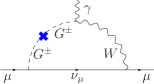
(a)

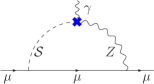
(b)

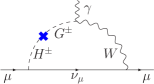
(c)

Figure 1: Counterterm Feynman diagrams.

We now turn to the counterterm diagrams. Fig. 1 shows sample diagrams. It is convenient to classify the 2HDM counterterm diagrams into three groups. The first group encompasses the SM-like counterterm diagrams without Higgs boson inside. The second group contains the counterterm diagrams with neutral physical Higgs bosons. The third group consists of the counterterm diagram with $G^{\pm}$-$H^{\pm}$ mixing counterterm vertex. In the following we explain them one after the other and provide the explicit results.

• SM-like counterterms without physical Higgs bosons:
  The first group encompasses the SM counterterm diagrams which do not contain physical Higgs bosons. The results of SM counterterm diagrams are found in Ref. [42]. The additional 2HDM contributions from these counterterm diagrams are obtained by applying the corresponding additional 2HDM renormalization constants. This is straightforward for all diagrams except Fig. 1(a). This diagram is the only one which contains the tadpole renormalization constants. In the following we explain the cancellation of the gauge and Goldstone boson contributions as well as the fermion contributions.

  The additional 2HDM contribution from this diagram is the difference between the 2HDM and SM results,

  $$a_{\mu}^{\text{CT }(GG)}= \frac{(\delta t_{GG}^{{\text{2HDM}}}-\delta t_{GG}^{\text{SM}})}{v}\frac{\alpha}{96\pi s_{\text{W}}^{2}}\frac{m_{\mu}^{2}}{M_{W}^{4}}\,\left\{2+\varepsilon\left(3-2\text{L}(M_{W}^{2})\right)\right\},$$ (37)

  where

  $$\text{L}(M^{2})\equiv\gamma_{E}-\ln(4\pi)+\ln(M^{2}/\mu^{2}).$$ (38)

  The counterterm vertices of the $G^{\pm}$-$G^{\pm}$ propagator for the SM and 2HDM are

  $$\delta t_{GG}^{\text{SM}}= \delta T_{\text{SM}},\quad\delta t_{GG}^{{\text{2HDM}}}=\cos(\beta-\alpha)\,\delta T_{H}+\sin(\beta-\alpha)\,\delta T_{h}.$$ (39)

  Hence, from Eqs. (36) and (39) we find that the tadpole renormalization constants with gauge/Goldstone bosons and fermion loops drop out from the result, Eq. (37). Consequently no new 2HDM contributions are obtained from the fermion, gauge boson, and Goldstone boson loops. The additional 2HDM contribution of Fig. 1(a) and all other diagrams of this group arises from the physical Higgs boson loop contributions to the tadpole, field and mass renormalization constants.

• Counterterm with neutral Higgs bosons:
  The second group of counterterm diagrams is shown in Fig. 1(b). These diagrams are dependent on Yukawa coupling and proportional to $\delta Z_{\text{ZA}}$, which is the same in both the SM and the 2HDM. The difference arises from the Yukawa coupling and the second neutral CP-even 2HDM Higgs boson. The fermionic loop contribution to $\delta Z_{\text{ZA}}$ are zero, therefore the diagrams of this group do not contribute to the fermion contributions.

  The additional 2HDM contribution is obtained when the SM Higgs boson contribution is subtracted from the 2HDM results, $a_{\mu}^{{\text{CT}}(H)}+a_{\mu}^{{\text{CT}}(h)}-a_{\mu}^{{\text{CT}}(h_{\text{SM}})}$, where the explicit result of Fig. 1(b) for an arbitrary scalar field ${\cal S}$ is

  $$a_{\mu}^{\text{CT}({\cal S})}= \,C_{\cal S}\,Y_{l}^{\cal S}\,\frac{\alpha}{32\pi}\frac{(1-4\,s_{\text{W}}^{2})}{c_{\text{W}}^{3}\,s_{\text{W}}^{3}}\frac{m_{\mu}^{2}}{(M_{\cal S}^{2}-M_{Z}^{2})^{2}}\,\delta Z_{\text{ZA}}$$

  $$\times\left\{M_{Z}^{2}-M_{\cal S}^{2}+M_{\cal S}^{2}\,\ln(M_{\cal S}^{2}/M_{Z}^{2})\right.$$

  $$\quad\,\,+\frac{\varepsilon}{2}\,(3(M_{Z}^{2}-M_{\cal S}^{2})+3\,M_{\cal S}^{2}\,\text{L}(M_{\cal S}^{2})-M_{\cal S}^{2}\,\text{L}(M_{\cal S}^{2})^{2}$$

  $$\left.\qquad\quad\,\,\,-(M_{\cal S}^{2}+2\,M_{Z}^{2})\,\text{L}(M_{Z}^{2})+M_{\cal S}^{2}\,\text{L}(M_{Z}^{2})^{2})\right\}.$$ (40)

  ${\cal S}$ can be any of the neutral Higgs bosons in the SM and the 2HDM: $h_{\text{SM}}$, $h$, $H$. The contribution of the CP-odd neutral Higgs $A$ is zero. The coefficient, $C_{\cal S}$, is derived from the gauge coupling. It is $1$ for the SM Higgs $h_{\text{SM}}$, $\sin(\beta-\alpha)$ for $h$ and $\cos(\beta-\alpha)$ for $H$. $Y_{l}^{\cal S}$ is derived from the Yukawa coupling constant and listed in Eq. (2.1). For the SM Higgs $h_{\text{SM}}$, $Y_{l}^{h_{\text{SM}}}=1$.

• Counterterm diagram with $G^{\pm}$-$H^{\pm}$ mixing:
  The third group consists of the diagram of Fig. 1(c) which is proportional to the $G^{\pm}$-$H^{\pm}$ mixing counterterm vertex. This counterterm diagram does not appear in the SM. The explicit analytic result reads

  $$a_{\mu}^{\text{CT }(GH)}= \frac{\delta t_{HG}}{v}\frac{\alpha}{16\pi s_{\text{W}}^{2}}\frac{m_{\mu}^{2}}{M_{W}\,(M_{W}^{2}-M_{H^{\pm}}^{2})^{3}}\,\zeta_{l}$$

  $$\times \bigg{[}(M_{H^{\pm}}^{4}-M_{W}^{4})\big{(}1+\varepsilon\,\text{L}(M_{W}^{2})\big{)}$$

  $$-M_{H^{\pm}}^{2}M_{W}^{2}\,\ln(M_{H^{\pm}}^{2}/M_{W}^{2})\big{(}2+\varepsilon\{3-\text{L}(M_{H^{\pm}}^{2})-\text{L}(M_{W}^{2})\}\big{)}$$

  $$+\frac{\varepsilon}{2}(M_{H^{\pm}}^{2}-M_{W}^{2})(M_{H^{\pm}}^{2}+5\,M_{W}^{2})\bigg{]}$$ (41)

  where $\delta t_{HG}=\cos(\beta-\alpha)\,\delta T_{h}-\sin(\beta-\alpha)\delta T_{H}$. $\zeta_{l}$-dependency arises from the charged Higgs boson coupling to the muon in the Aligned 2HDM. Fig. 1(c) is the only counterterm diagram which contributes to the fermionic two-loop result.

3.3 Bosonic loop contribution

3.3.1 2-boson and 3-boson diagrams

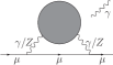
(a)

(b)

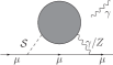
(c)

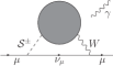
(d)

Figure 2: Generic 2-boson Feynman diagrams. The gray loops denote any bosonic loop.

(a)

(b)

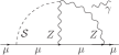
(c)

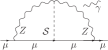
(d)

Figure 3: 3-boson Feynman diagrams are mediated either with $W$ or $Z$ bosons. They contain only the neutral physical CP-even Higgs bosons.

We classify the bosonic two-loop diagrams according to the number of bosons coupling to the muon line. With this criterion it is possible to group the diagrams into 2-boson and 3-boson types. The 2-boson type denotes all diagrams in which two internal bosons couple to the muon line. The generic diagrams of the 2-boson diagrams are shown in Fig. 2. Gray circles in Fig. 2 denote all possible bosonic loops. These 2-boson diagrams contain the so-called Barr-Zee diagrams, which have already been computed and intensively discussed in the literature [39, 46, 47, 45, 48, 30]. The 2-boson diagrams also contain self-energy type diagrams in which the external photon couples to the muon line.

The 3-boson diagrams have a more complicated structure and involve three internal bosons which couple to the muon line. Fig. 3 shows all 3-boson diagrams which contribute to the difference between the 2HDM and the SM. In addition, diagrams with four bosons coupling to the muon line exist but do not contribute to the difference between the SM and 2HDM at the order of ${\cal O}(m_{\mu}^{2})$.

We especially computed the 3-boson diagrams shown in Fig. 3 for the first time. Figs. 3(a) and 3(b) are dependent on the $W$ boson and Figs. 3(c) and 3(d) on the $Z$ boson. While computing the diagrams in Fig. 3, we should pay attention to two interactions. One is the muon Yukawa coupling to the neutral scalar bosons, $h$ or $H$, and the other is the Higgs-gauge interaction of the two neutral Higgs bosons. The gauge interaction to $H$ is suppressed by $\eta$. In the SM-limit the contribution from this interaction becomes zero, whereas the gauge interaction to $h$ recovers the SM value. The explicit result of Figs. 3(a) and 3(b) reads

$$a_{\mu}^{W,{\cal S}}= C_{\cal S}Y_{l}^{\cal S}\frac{\alpha^{2}}{576\,\pi^{2}\,c_{\text{W}}^{4}s_{\text{W}}^{4}}\,\frac{m_{\mu}^{2}}{M_{Z}^{2}}\Big{\{}\frac{3}{\varepsilon}-6\text{L}(M_{W}^{2})-\frac{55}{2}+\frac{32}{y_{\cal S}}-\frac{4\pi^{2}}{3}\Big{(}\frac{4+3y_{\cal S}}{y_{\cal S}^{2}}\Big{)}$$

$$-\Big{(}35+\frac{32}{y_{\cal S}}\Big{)}\ln(y_{\cal S})+\Big{(}6+\frac{32}{y_{\cal S}^{2}}+\frac{24}{y_{\cal S}}-32y_{\cal S}\Big{)}\text{Li}_{2}(1-y_{\cal S})$$

$$+\Big{(}\frac{10+70y_{\cal S}-32y_{\cal S}^{2}}{(y_{\cal S}-4)y_{\cal S}}\Big{)}{\Phi}(\sqrt{y_{\cal S}},1,1),$$ (42)

where $S\in{h,H}$, and $y_{\cal S}\equiv\frac{M_{\cal S}^{2}}{M_{W}^{2}}$. ${\Phi}(x,y,z)$ is defined in Appendix A. We have $C_{h}=1$, $Y_{l}^{h}=1+\eta\zeta_{l}$ for $h$ and $C_{H}=\eta$, $Y_{l}^{H}=\eta-\zeta_{l}$ for $H$ up to ${\cal O}(\eta)$. For the SM Higgs boson, $Y_{l}^{h_{\text{SM}}}=1$, and $C_{h_{\text{SM}}}=1$. The divergent part of Eq. (3.3.1) drops out in the final result of the difference of the SM and 2HDM. Note that the result of Fig. 3(b) alone is finite. In the off-SM scenario, $\eta\neq 0$, the result of Fig. 3 for ${\cal S}=h$ results in additional EW contributions.

The additional 2HDM contribution from the diagrams of Figs. 3(a) and 3(b) is obtained when the SM Higgs boson result of Eq. (3.3.1) is subtracted from the sum of the $h$ and $H$ contributions, $a_{\mu}^{W,h}+a_{\mu}^{W,H}-a_{\mu}^{W,h_{\text{SM}}}$. After employing the known SM parameters we obtain the numerical result

$$a_{\mu}^{W,H}+a_{\mu}^{W,h}-a_{\mu}^{W,h_{\text{SM}}}=(3\cdots-4.6)\times 10^{-12}\,\eta\zeta_{l},$$ (43)

for $50<M_{H}<500\;{\text{GeV}}$ and $M_{h}=M_{h_{\text{SM}}}=125\;{\text{GeV}}$. The maximum value of Eq. (43) for a fixed $\eta\zeta_{l}$ is $|-5.1\eta\zeta_{l}|\times 10^{-12}$ for $M_{H}\sim 950\;{\text{GeV}}$. Eq. (43) vanishes when $M_{H}=M_{h}$.

For the case of $Z$ boson dependent non Barr-Zee diagrams, Figs. 3(c) and 3(d), the analytic result for an arbitrary Higgs boson ${\cal S}$ reads

$$a_{\mu}^{Z,{\cal S}}= C_{\cal S}Y_{l}^{\cal S}\frac{\alpha^{2}}{576\,\pi^{2}\,c_{\text{W}}^{4}s_{\text{W}}^{4}}\,\frac{m_{\mu}^{2}}{M_{Z}^{2}}\Big{(}f_{a}(x_{\cal S})+s_{\text{W}}^{2}(1-2s_{\text{W}}^{2})f_{b}(x_{\cal S})\Big{)},$$ (44)

$$f_{a}(x_{\cal S})= \frac{3(4-x_{\cal S})}{x_{\cal S}}-\frac{\pi^{2}}{2}\Big{(}\frac{4+3x_{\cal S}}{x_{\cal S}^{2}}\Big{)}-\frac{3(4+x_{\cal S})}{x_{\cal S}}\ln(x_{\cal S})$$

$$+\frac{12+9x_{\cal S}-3x_{\cal S}^{3}}{x_{\cal S}^{2}}\text{Li}_{2}(1-x_{\cal S})+\frac{3(2+x_{\cal S})}{x_{\cal S}}{\Phi}(\sqrt{x_{\cal S}},1,1),$$ (45)

$$f_{b}(x_{\cal S})= \frac{\pi^{2}(8+6x_{\cal S}-12x_{\cal S}^{4}+3x_{\cal S}^{5})}{x_{\cal S}^{2}}+\frac{6(-8+2x_{\cal S}+3x_{\cal S}^{2})}{x_{\cal S}}$$

$$+\frac{12(4+x_{\cal S}+3x_{\cal S}^{2})}{x_{\cal S}}\ln(x_{\cal S})+9(-4+x_{\cal S})x_{\cal S}^{2}\ln(x_{\cal S})^{2}$$

$$+\frac{12(-4-3x_{\cal S}+4x_{\cal S}^{3}-12x_{\cal S}^{4}+3x_{\cal S}^{5})}{x_{\cal S}^{2}}\text{Li}_{2}(1-x_{\cal S})$$

$$+\frac{6(4+2x_{\cal S}-6x_{\cal S}^{2}+3x_{\cal S}^{3})}{x_{\cal S}}{\Phi}(\sqrt{x_{\cal S}},1,1),$$ (46)

and $x_{\cal S}\equiv\frac{M_{\cal S}^{2}}{M_{Z}^{2}}$. $C_{\cal S}$ and $Y_{l}^{\cal S}$ for $h$ and $H$ are the same as in Eq. (3.3.1).

Like Eq. (43) the additional 2HDM contribution from the diagrams of Figs. 3(c) and 3(d) is obtained as

$$a_{\mu}^{Z,H}+a_{\mu}^{Z,h}-a_{\mu}^{Z,h_{\text{SM}}}=(5.6\cdots-5.6)\times 10^{-13}\eta\zeta_{l},$$ (47)

for $50<M_{H}<500\;{\text{GeV}}$ and $M_{h}=M_{h_{\text{SM}}}=125\;\text{GeV}$. When $M_{H}>125\;{\text{GeV}}$, Eq. (47) becomes negative. The W boson result is approximately a factor 10 larger than the Z boson result; it can become significant for large values of $\zeta_{l}$ and $\eta$.

3.3.2 Analytic results

In this section we present the complete renormalized bosonic 2HDM contribution. The bosonic result is expanded with respect to the parameter $\eta$ introduced in Sec. 2, and terms up to $\eta^{1}$ are taken. In the SM-limit, $\eta\to 0$, the interactions of $h$ to the gauge bosons or fermions become just those of the SM.

For the discussion of the complete result we do not use the 2-boson and 3-boson separation. Instead, we divide the renormalized bosonic contribution into two parts. One part, $a_{\mu}^{\text{EW add.}}$, is defined by the Feynman diagrams containing only gauge/Goldstone/$h$ bosons, i.e. purely SM-like diagrams. The other part is defined by those diagrams which include at least one of the new 2HDM Higgs bosons, $H,A,H^{\pm}$. This part can be again divided into Yukawa-dependent and Yukawa-independent parts. Considering this classification we can write the bosonic contribution as

$$a_{\mu}^{\text{B}}= a_{\mu}^{\text{EW add.}}+a_{\mu}^{\text{non-Yuk}}+a_{\mu}^{\text{Yuk}},$$ (48)

where $a_{\mu}^{\text{non-Yuk}}$ denotes Yukawa-independent 2HDM Higgs contributing part and $a_{\mu}^{\text{Yuk}}$ the Yukawa-dependent part. In the following we explain each of the contributions explicitly.

• $a_{\mu}^{\text{EW add.}}$
  We start with the computation of $a_{\mu}^{\text{EW add.}}$. The additional 2HDM EW contribution, $a_{\mu}^{\text{EW add.}}$ is obtained by subtracting the Feynman diagram result with SM physical Higgs boson $h_{\text{SM}}$ from the 2HDM diagrams which include only $h$. The diagrams of Fig. 2(c) and Fig. 3 with ${\cal S}=h$ contribute to this difference at the order $\eta\zeta_{l}$ due to the different Yukawa couplings in the two models. The diagrams of Figs. 2(a) and 2(b) as well as Fig. 2(d) with charged Goldstone boson, ${\cal S}^{\pm}=G^{\pm}$ and with $h$ in the gray loop also contribute to $a_{\mu}^{\text{EW add.}}$, however only starting at the order $\eta^{2}$; hence we neglect them. The only counterterm diagram contributing to $a_{\mu}^{\text{EW add.}}$ is the diagram of Fig. 1(b) with $h$.

  After summing up the two-loop and the counterterm results and employing the SM parameters we obtain finally the complete result

  $$a_{\mu}^{\text{EW add.}}= 2.3\times 10^{-11}\,\eta\,\zeta_{l}.$$ (49)

  The sign of $a_{\mu}^{\text{EW add.}}$ is dependent on $\eta\,\zeta_{l}$. Even though $\eta$ must be small, the appearance of $\zeta_{l}$ can enhance the contribution of $a_{\mu}^{\text{EW add.}}$.

• $a_{\mu}^{\text{non-Yuk}}$
  Now we turn to $a_{\mu}^{\text{non-Yuk}}$ in Eq. (48).

  

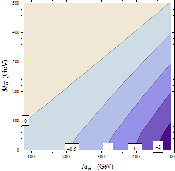
  (a) $M_{A}=10\;\text{GeV}$

  

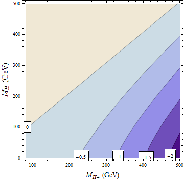
  (b) $M_{A}=50\;\text{GeV}$

  

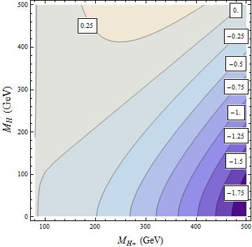
  (c) $M_{A}=100\;\text{GeV}$

  

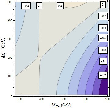
  (d) $M_{A}=200\;\text{GeV}$

  Figure 4: Plots of $a_{\mu}^{\text{non-Yuk}}$ for different values of $M_{A}=10,50,100,200\;\text{GeV}$. The results should be multiplied by a factor $10^{-10}$. The contour line value for fixed $M_{H}$ and $M_{H^{\pm}}$ decreases as $M_{A}$ increases. As $M_{A}$ becomes larger, $a_{\mu}^{\text{non-Yuk}}$ becomes more sensitive to the difference of the neutral and charged Higgs boson masses: compare the right-bottom areas of the plots. For a given $M_{A}$ value $|a_{\mu}^{\text{non-Yuk}}|$ increases as $M_{H^{\pm}}-M_{H}$ becomes larger.

  It comes from the Feynman diagrams without Yukawa couplings containing at least one of the new 2HDM physical Higgs bosons, $H,A,H^{\pm}$. The Feynman diagrams of Figs. 2(a) and 2(b) with $H/A/H^{\pm}$ in the gray loops contribute to $a_{\mu}^{\text{non-Yuk}}$.

  $a_{\mu}^{\text{non-Yuk}}$ is dependent on parameters, $M_{H}$, $M_{A}$, and $M_{H^{\pm}}$, but not on $t_{\beta}$ and $\Lambda_{5}$. It also does not gain terms linearly dependent on the parameter $\eta$. We should stress that $a_{\mu}^{\text{non-Yuk}}$ is the only part dependent on $M_{A}$ in the bosonic contributions. The explicit analytic result is found in Appendix A.

  Fig. 4 shows the change of $a_{\mu}^{\text{non-Yuk}}$ for different $M_{A}$ values. For $M_{A}<100\;{\text{GeV}}$ and $M_{H},M_{H^{\pm}}>100\;{\text{GeV}}$, $a_{\mu}^{\text{non-Yuk}}$ has the same sign of the difference between $M_{H}$ and $M_{H^{\pm}}$. $a_{\mu}^{\text{non-Yuk}}$ depends mainly on the difference between the masses of the three Higgs bosons. In the largest part of the parameter space in the Figure, $a_{\mu}^{\text{non-Yuk}}$ is negative and amounts up to $-2\,\times\,10^{-10}$.

• $a_{\mu}^{\text{Yuk}}$
  The terms contained in $a_{\mu}^{\text{Yuk}}$ in Eq. (48) are from those diagrams with Yukawa contributions and the corresponding counterterms.

  

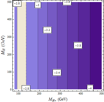
  (a) $a_{0,0}^{0}$

  

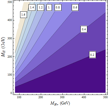
  (b) $a_{0,z}^{0}$

  

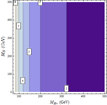
  (c) $a_{5,0}^{0}$

  

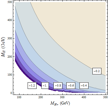
  (d) $a_{5,z}^{0}$

  Figure 5: Plots of the $\eta^{0}$-order coefficients, $a_{i,j}^{0}$ in Eq. (• ‣ 3.3.2). The values of contour lines should be multiplied by $10^{-12}$. The values of these plots are not suppressed by $\eta$. $a_{0,0}^{0}$ and $a_{5,0}^{0}$ are only dependent on $M_{H^{\pm}}$. On the given parameter space $a_{0,0}^{0}$ is negative whereas $a_{5,0}^{0}$ positive. As $M_{H^{\pm}}$ increases, $|a_{0,0}^{0}|$ increases, but $|a_{5,0}^{0}|$ decreases. Although the magnitudes of $|a_{0,z}^{0}|$ and $|a_{5,z}^{0}|$ are smaller than those of $a_{0,0}^{0}$ and $a_{5,0}^{0}$, they are enhanced by large $t_{\beta}$ and $\zeta_{l}$.

  Among the 2-boson diagrams the Feynman diagrams of Figs. 2(c) and 2(d) with ${\cal S}=H$ and ${\cal S}^{\pm}=H^{\pm}$ contribute to $a_{\mu}^{\text{Yuk}}$. The diagrams of Fig. 2(c) also contribute if ${\cal S}=h$ and the gray loop contains at least one of the new physical 2HDM Higgs bosons. These diagrams include triple or quartic scalar boson couplings. The 3-boson diagrams of Fig. 3 with $H$ contribute to $a_{\mu}^{\text{Yuk}}$, too.

  Clearly, all diagrams with $H$ or $H^{\pm}$ and gauge bosons are suppressed by $\eta$ but enhanced by $\zeta_{l}$. The diagrams without gauge bosons involve triple Higgs couplings and are of particular interest. A closer look at the triple Higgs coupling constants helps to analyze the $t_{\beta}$-dependency. The triple Higgs couplings constants in the 2HDM are

  $$g_{h,H^{\pm},H^{\mp}}\propto \left\{v\,\left(\Lambda_{5}-\frac{M_{h}^{2}}{v^{2}}-2\frac{M_{H^{\pm}}^{2}}{v^{2}}\right)\right.$$

  $$\left.\,\,+\,\eta\,\left(t_{\beta}-\frac{1}{t_{\beta}}\right)\frac{v}{2}\left(2\,\frac{M_{h}^{2}}{v^{2}}-\Lambda_{5}\right)\right\}$$ (50)

  $$g_{H,H^{\pm},H^{\mp}}\propto \left\{\left(t_{\beta}-\frac{1}{t_{\beta}}\right)\frac{v}{2}\left(\Lambda_{5}-2\,\frac{M_{H}^{2}}{v^{2}}\right)\right.$$

  $$\left.\,\,+\eta\,v\left(\Lambda_{5}-\frac{M_{H}^{2}}{v^{2}}-2\frac{M_{H^{\pm}}^{2}}{v^{2}}\right)\right\}$$ (51)

  The triple Higgs coupling constants show that the $t_{\beta}$-dependency comes only in the form of $(t_{\beta}-\frac{1}{t_{\beta}})$, which leads to a large $t_{\beta}$-enhancement. In the actual Feynman diagrams with triple Higgs couplings, the coupling Eq. (• ‣ 3.3.2) appears multiplied with $Y_{l}^{h}$, and the coupling Eq. (• ‣ 3.3.2) is multiplied with $Y_{l}^{H}$ and $Y_{l}^{A}$. This allows to read off which combinations of the parameters $\zeta_{l}$, $\eta$, $\Lambda_{5}$ appear in these diagrams. With these considerations, we can rewrite $a_{\mu}^{\text{Yuk}}$ as

  $$a_{\mu}^{\text{Yuk}}= a_{0,0}^{0}+a_{0,z}^{0}\,\left(t_{\beta}-\frac{1}{t_{\beta}}\right)\,\zeta_{l}+a_{5,0}^{0}\,\Lambda_{5}+a_{5,z}^{0}\,\left(t_{\beta}-\frac{1}{t_{\beta}}\right)\,\Lambda_{5}\,\zeta_{l}+$$

  $$+ \left(a_{0,0}^{1}\,\left(t_{\beta}-\frac{1}{t_{\beta}}\right)+a_{0,z}^{1}\,\zeta_{l}+a_{5,0}^{1}\,\left(t_{\beta}-\frac{1}{t_{\beta}}\right)\,\Lambda_{5}+a_{5,z}^{1}\,\Lambda_{5}\,\zeta_{l}\right)\,\eta.$$ (52)

  The notation is such that the terms with superscript ⁰ are independent of $\eta$, the terms with superscript ¹ are linear in $\eta$. The subscript _z denotes terms enhanced by $\zeta_{l}$, the subscript ₅ denotes terms $\propto\Lambda_{5}$. All terms here arise from diagrams with triple Higgs couplings except the $a_{0,z}^{1}$ term. The results of the 3-boson diagrams Eqs. (3.3.1) and (44) for $H$ are included in $a_{0,z}^{1}$. The parameter dependence of each coefficient $a_{i,j}^{k}$ is rather simple. $a_{0,0}^{0}$ and $a_{5,0}^{0}$ are dependent only on $M_{H^{\pm}}$ and the rest dependent only on $M_{H}$ and $M_{H^{\pm}}$. In Appendix A we present the explicit expression of the coefficients $a_{i,j}^{k}$ as well as $a_{\mu}^{\text{non-Yuk}}$, and in Appendix B we show that there is no dependence on $M_{A}$.

  The plots in Fig. 5 show the complete mass dependence of the coefficients $a^{0}_{i,j}$. $a_{0,0}^{0}$ and $a_{5,0}^{0}$ arise from the Feynman diagrams containing the muon Yukawa interaction to $h$ and the $\eta$-independent part of Eq. (• ‣ 3.3.2), therefore are dependent only on $M_{H^{\pm}}$ and neither enhanced by $t_{\beta}$ nor by $\zeta_{l}$. In contrast, $a_{0,z}^{0}$ and $a_{5,z}^{0}$ arise from diagrams involving the triple Higgs coupling Eq. (• ‣ 3.3.2) and appear enhanced by large $t_{\beta}$ and $\zeta_{l}$ in Eq. (• ‣ 3.3.2).

  The plots in Fig. 6 show the change of $a_{0,0}^{1}$, $a_{0,z}^{1}$, $a_{5,0}^{1}$ and $a_{5,z}^{1}$, the $\eta$-suppressed terms. The coefficient $a_{0,z}^{1}$, which gets contributions from a larger class of diagrams, can be numerically larger than the other coefficients.

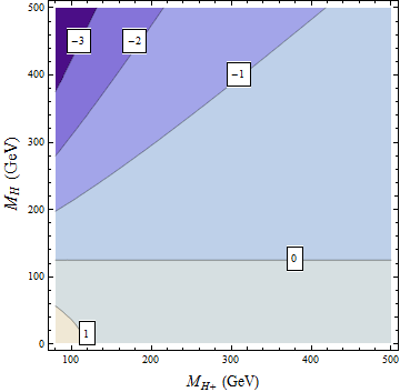
(a) $a_{0,0}^{1}$

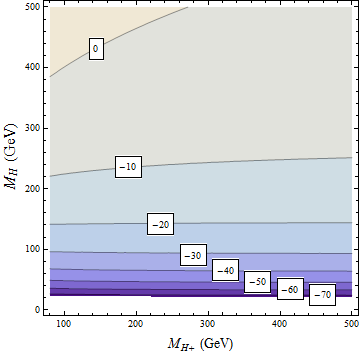
(b) $a_{0,z}^{1}$

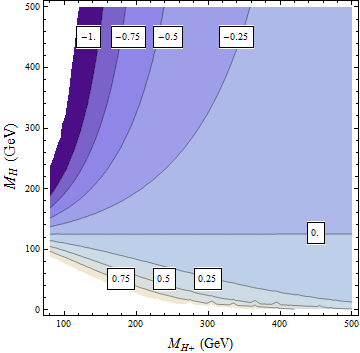
(c) $a_{5,0}^{1}$

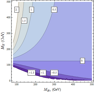
(d) $a_{5,z}^{1}$

Figure 6: Plots of $a_{0,0}^{1}$, $a_{0,z}^{1}$, $a_{5,0}^{1}$ and $a_{5,z}^{1}$. The results must be multiplied by a factor $10^{-12}$. Terms with these coefficients in Eq. (• ‣ 3.3.2) are suppressed by $\eta$. $a_{0,0}^{1}$ and $a_{5,0}^{1}$ are enhanced by large $t_{\beta}$ whereas $a_{0,z}^{1}$ and $a_{5,z}^{1}$ by $\zeta_{l}$.

3.4 Fermionic loop contribution

In this section we present the fermionic loop contribution to $a_{\mu}$. Due to the higher order muon mass suppression (considering terms up to $m_{\mu}^{2}$ order), all diagrams contain only one scalar boson, which interacts with the incoming/outgoing muon and the fermion in the inner loop. Thus, the result is always proportional to the product of two Yukawa couplings $Y^{\cal S}_{l}Y^{\cal S}_{f}$.

The fermionic two-loop Feynman diagrams contain either neutral or charged Higgs bosons. Fig. 7(a) shows the generic diagrams for neutral Higgs bosons while Fig. 7(b) is related to charged bosons. When the external photon couples with the muon line we obtain self-energy type diagrams, and the sum of these vanishes. The remaining diagrams are Barr-Zee diagrams.

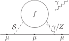
(a)

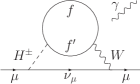
(b)

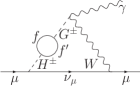
(c)

Figure 7: (a)Generic two-loop diagram with fermion loops and neutral Higgs bosons. The photon can couple with any charged particle inside. When the photon couples with the fermion loop, we obtain Barr-Zee diagrams. (b) Generic fermionic two-loop diagram with charged Higgs bosons. Barr-Zee diagrams are diagrams where the photon generates an effective photon-vector-scalar interaction. (c) $\gamma\,W\,G^{\pm}$ vertex diagram with charged Higgs bosons.

Our result for neutral Higgs bosons is coincident with previous analysis [36, 37, 30], and the explicit form is

$$a_{\mu}^{\text{F, N}} =\sum_{{\cal S}=\{h,H,A\}}\sum_{f=\{u,d,l\}}\left[f^{\cal S}_{f}(M_{\cal S},m_{f})\right]Y^{\cal S}_{f}Y^{\cal S}_{l}$$

$$\equiv\sum_{{\cal S}=\{h,H,A\}}\sum_{f=\{u,d,l\}}\left[f^{\gamma}_{\cal S}(M_{\cal S},m_{f})+f^{Z}_{\cal S}(M_{\cal S},m_{f})\right]Y^{\cal S}_{f}Y^{\cal S}_{l},$$ (53)

where

$$f^{\gamma}_{\cal S}(M_{\cal S},m_{f})= \frac{\alpha^{2}m^{2}_{\mu}}{4\pi^{2}M_{W}^{2}s_{\text{W}}^{2}}\left(Q_{f}^{2}N_{c}^{f}\right)\left(\frac{m_{f}^{2}}{M_{\cal S}^{2}}\right)\mathcal{F}_{\cal S}(M_{\cal S},m_{f}),$$ (54)

$$f^{Z}_{\cal S}(M_{\cal S},m_{f})= \frac{\alpha^{2}m^{2}_{\mu}}{4\pi^{2}M_{W}^{2}s_{\text{W}}^{2}}\left(-\frac{N_{c}^{f}Q_{f}g_{v}^{l}g_{v}^{f}}{s_{\text{W}}^{2}c_{\text{W}}^{2}}\right)$$

$$\times\frac{m^{2}_{f}}{(M_{\cal S}^{2}-M_{Z}^{2})}\left[\mathcal{F}_{\cal S}(M_{\cal S},m_{f})-\mathcal{F}_{\cal S}(M_{Z},m_{f})\right].$$ (55)

For ${\cal S}=\{h,H\}$ we have

$$\mathcal{F}_{\cal S}(M_{\cal S},m_{f}) =-2+\ln\left(\frac{M_{\cal S}^{2}}{m_{f}^{2}}\right)-\left(\frac{M_{\cal S}^{2}-2m_{f}^{2}}{M_{\cal S}^{2}}\right)\,\frac{{\Phi}(M_{\cal S},m_{f},m_{f})}{M_{\cal S}^{2}-4m_{f}^{2}},$$ (56)

and for ${\cal S}=A$

$$\mathcal{F}_{\cal S}(M_{\cal S},m_{f}) =\frac{{\Phi}(M_{\cal S},m_{f},m_{f})}{M_{\cal S}^{2}-4m_{f}^{2}}.$$ (57)

A sum over all types of fermions is implicit. $Q_{f}$ denotes the charge of the respective fermion $f$, and $N_{c}^{f}$ the color factor. We also define $g_{v}^{f}\equiv\frac{T_{3}}{2}-Q_{f}s_{\text{W}}^{2}$, and ${\Phi}(M_{\cal S},m_{f},m_{f})$ is defined in Appendix A. Both $\gamma$ and $Z$ bosons contribute to the fermionic loop result with neutral Higgs bosons. However, the result from the $Z$ boson is suppressed by factor $g_{v}^{f}$, which is $-1/4+s_{\text{W}}^{2}\sim-0.02$ for leptons, compared to the result from the diagrams with photon. Hence the $Z$ contributions are always smaller than those of the photon.

Now we turn to the fermionic two-loop contributions with charged Higgs bosons. Figs. 7(b) and 7(c) show the corresponding Feynman diagrams. Especially the result of Fig. 7(c) is divergent, the corresponding counterterm diagram is shown in Fig. 1(c). The renormalized two-loop result is obtained by summing up the two-loop and the counterterm diagrams. These diagrams were computed in the context of SUSY models long ago [46, 47] in which case a type II structure for the Yukawas needed to be assumed. In the case of a general model (Aligned Model, for instance) the analysis was only recently performed [30]. We also recover the analytic result presented in [46, 47, 30], explicitly

$$a_{\mu}^{\text{F,C}}=\sum_{f=\{u,d,l\}}f^{H^{\pm}}_{f}(M_{H^{\pm}},M_{f})Y^{A}_{f}Y^{A}_{l},$$ (58)

where $M_{f}$ corresponds to pairs of fermions masses as $M_{u}=\{(m_{u},m_{d}),(m_{c},m_{s}),(m_{t},m_{b})\}$, $M_{d}=M_{u}$, $M_{l}=\{(m_{e},0),(m_{\mu},0),(m_{\tau},0)\}$, and Eq. (58) contains an implicit sum over pairs. We neglect neutrino masses and generation mixing. We also introduced the definitions below in Eq. (58)

$$f^{H^{\pm}}_{f}(M_{H^{\pm}},M_{f})=\frac{\alpha^{2}m^{2}_{\mu}}{32\pi^{2}M_{W}^{2}s_{\text{W}}^{4}}\frac{N^{f}_{c}m_{f}^{2}}{(M_{H^{\pm}}^{2}-M_{W}^{2})}\left[\mathcal{F}^{H^{\pm}}_{f}(M_{f})-(M_{H^{\pm}}\rightarrow M_{W})\right],$$ (59)

$$x_{f}\equiv\frac{m^{2}_{f}}{M_{H^{\pm}}^{2}},\quad y\equiv\left(x_{u}-x_{d}\right)^{2}-2\left(x_{u}+x_{d}\right)+1,\quad s\equiv\frac{(Q_{u}+Q_{d})}{4}$$

$$c\equiv\left[\left(x_{u}-x_{d}\right)^{2}-Q_{u}x_{u}+Q_{d}x_{d}\right],\quad\mathrm{bar}{c}\equiv\left[\left(x_{u}-Q_{u}\right)x_{u}-\left(x_{d}+Q_{d}\right)x_{d}\right],$$

$$\mathcal{F}^{H^{\pm}}_{l}(M_{l})=x_{l}+x_{l}\left(x_{l}-1\right)\left[\mbox{Li}_{2}(1-1/x_{l})-\frac{\pi^{2}}{6}\right]+\left(x_{l}-\frac{1}{2}\right)\ln(x_{l}),$$ (60)

$$\mathcal{F}^{H^{\pm}}_{d}(M_{d})=-(x_{u}-x_{d})+\left[\frac{\mathrm{bar}{c}}{y}-c\left(\frac{x_{u}-x_{d}}{y}\right)\right]{\Phi}(x_{d}^{1/2},x_{u}^{1/2},1)$$

$$\quad\quad\quad\quad\quad\quad+c\left[\mbox{Li}_{2}\left(1-\frac{x_{d}}{x_{u}}\right)-\frac{1}{2}\ln(x_{u})\ln\left(\frac{x_{d}}{x_{u}}\right)\right]$$

$$\quad\quad\quad\quad\quad\quad+\left(s+x_{d}\right)\ln(x_{d})+\left(s-x_{u}\right)\ln(x_{u}),$$ (61)

$$\mathcal{F}^{H^{\pm}}_{u}(M_{u})=\mathcal{F}^{H^{\pm}}_{d}(x_{u},x_{d})\left(Q_{u}\rightarrow 2+Q_{u},Q_{d}\rightarrow 2+Q_{d}\right)$$

$$\quad\quad\quad\quad\quad\quad-\frac{4}{3}\left(\frac{x_{u}-x_{d}-1}{y}\right){\Phi}(x_{d}^{1/2},x_{u}^{1/2},1)$$

$$\quad\quad\quad\quad\quad\quad-\frac{1}{3}\left[\ln^{2}(x_{d})-\ln^{2}(x_{u})\right].$$ (62)

Summing the results of Eqs. (53) and (58) and subtracting the corresponding SM-Higgs contribution gives the full renormalized two-loop 2HDM fermionic contribution

$$a_{\mu}^{\text{F}}=\sum_{f=\{u,d,l\}}\Bigg{[}\sum_{{\cal S}=\{h,H,A\}}f_{f}^{\cal S}(M_{\cal S},m_{f})Y^{\cal S}_{f}Y^{\cal S}_{l} +f^{H^{\pm}}_{f}(M_{H^{\pm}},M_{f})Y^{A}_{f}Y^{A}_{l}$$

$$-f_{f}^{h_{\text{SM}}}(M_{h_{\text{SM}}},m_{f})\Bigg{]}.$$ (63)

After applying the Aligned 2HDM Yukawa coupling constants in Eq. (2.1) we can rewrite Eq. (63) with $\zeta_{f}$, and the result reads

$$a_{\mu}^{\text{F}}= \sum_{f=\{u,d,l\}}\left[\sum_{{\cal S}=\{H,A\}}\Theta^{\cal S}_{f}f_{f}^{\cal S}(M_{\cal S},m_{f})\zeta_{f}\zeta_{l}+\Theta^{A}_{f}f^{H^{\pm}}_{f}(M_{H^{\pm}},M_{f})\zeta_{f}\zeta_{l}\right]$$

$$+\sum_{f=\{u,d,l\}}\left[\eta\left(f_{f}^{h}(M_{h},m_{f})-f_{f}^{H}(M_{H},m_{f})\right)\left(\zeta_{f}+\zeta_{l}\right)\right],$$ (64)

where $\Theta^{A}_{u}=-1$, otherwise $\Theta^{\cal S}_{f}=1$. Each function $f_{f}^{i}(M_{i})$ in Eq. (64) is dependent on only one mass parameter, $M_{\cal S}$, and this enables us to analyze the individual Higgs boson contributions to the fermionic loop contribution in Fig. 8. The first line of Eq. (64) contains terms bilinear in the $\zeta_{f}$, and they are shown in the first three plots of Fig. 8. The terms in the second line are proportional to $\zeta_{f}\eta$ and are illustrated in the fourth plot, Fig. 8(d).

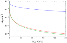
(a)

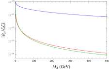
(b)

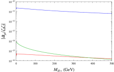
(c)

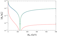
(d)

Figure 8: Fermionic contributions to $a_{\mu}$. The blue/red/green line refers to diagrams proportional to $\zeta_{u}$/$\zeta_{d}$/$\zeta_{l}$, respectively. The first three graphs (a)–(c) show the contributions with $H$, $A$, $H^{\pm}$ at order $\eta^{0}$. The plot (d) shows the corrections at $\eta$ order from diagrams with CP-even bosons.

In all cases the contribution from the top loop (blue line) is significantly larger, as expected by the factor $m_{t}^{2}/(M_{\cal S}^{2}-M_{B}^{2})$ in the analytic formulas ($M_{B}$ is the mass of the internal gauge boson involved). However, as discussed in Sec. 2.2.2, $\zeta_{u}$ is constrained to be at most $\zeta_{u}\simeq 1$, meaning that the tau loop, enhanced by $\zeta_{l}^{2}$, plays the decisive role. Another characteristic shared by Figs. 8(a) – 8(c) is that they all decrease with the mass of the scalars. Fig. 8(d) shows the contribution proportional to $\eta$ which comes from diagrams involving CP-even scalar bosons. As presented in Eq. (64) there is a difference between the $h$ and $H$ results, explaining why the $\eta^{1}$ contribution vanishes as $M_{h}$ approaches $M_{H}$. For all plots, we have rescaled $a_{\mu}$ to the aligned parameters. Finally, in all graphs the contributions can be both positive or negative. The signs depend on the alignment parameters and can be read off from Table 3.

	$f^{H}$	$f^{A}$	$f^{H^{\pm}}$
$\zeta_{u}\zeta_{l}$	$-$	$-$	$-$
$\zeta_{d}\zeta_{l}$	$-$	$+$	$-$
$\zeta_{l}^{2}$	$-$	$+$	$+$

	$m_{H}<m_{h}$	$m_{h}<m_{H}$
$\eta\zeta_{u}$	$+$	$-$
$\eta\zeta_{d}$	$+$	$-$
$\eta\zeta_{l}$	$+$	$-$

Table 3: Relation between signs of the aligned parameters and the functions depicted in Fig. 8.

4 Numerical Analysis

In this section we present the numerical analysis of our result. Our aim is to study how large the bosonic contribution, fully computed for the first time, can be. We will show that there are regions of the parameter space in which $a_{\mu}^{\text{B}}$ amounts to $(2\cdots 4)\times 10^{-10}$. Although always smaller than the fermionic contribution, it proves to be relevant for a precise determination of the 2HDM contribution to the muon anomalous magnetic moment. We also analyze the impact of deviations from the SM-limit by studying different values for the expansion parameter $\eta$.

For the analysis we choose physical free input parameters, the masses of the different scalars ($M_{H}$, $M_{A}$, $M_{H^{\pm}}$), the alignment parameters ($\zeta_{l,u,d}$), $t_{\beta}$, the expansion parameter $\eta$, and $\Lambda_{5}$. As presented in Sec. 2, the last parameter can be expressed in terms of $\lambda_{1}$, which is directly constrained by stability and perturbativity. Therefore, for the numerical analysis, it will be useful to replace the parameter $\Lambda_{5}$ with $\lambda_{1}$. As discussed in Sec. 2.2 we adopt the following allowed range for the parameters,

$$125<M_{H}<500\;\text{GeV},\quad M_{A}<500\;\text{GeV},\quad 80<M_{H^{\pm}}<500\;\text{GeV},$$

$$0<|\zeta_{u}|<1.2,\qquad\quad 0<|\zeta_{d}|<50,\quad\,0<|\zeta_{l}|<100,$$

$$1<t_{\beta}<100,\qquad\quad\,\,0<|\eta|<0.1,\quad\,0<\lambda_{1}<4\pi.$$ (65)

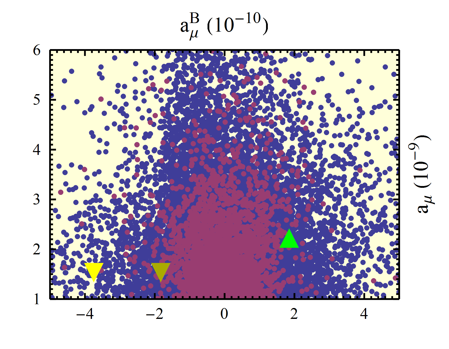
(a) $\eta=0$

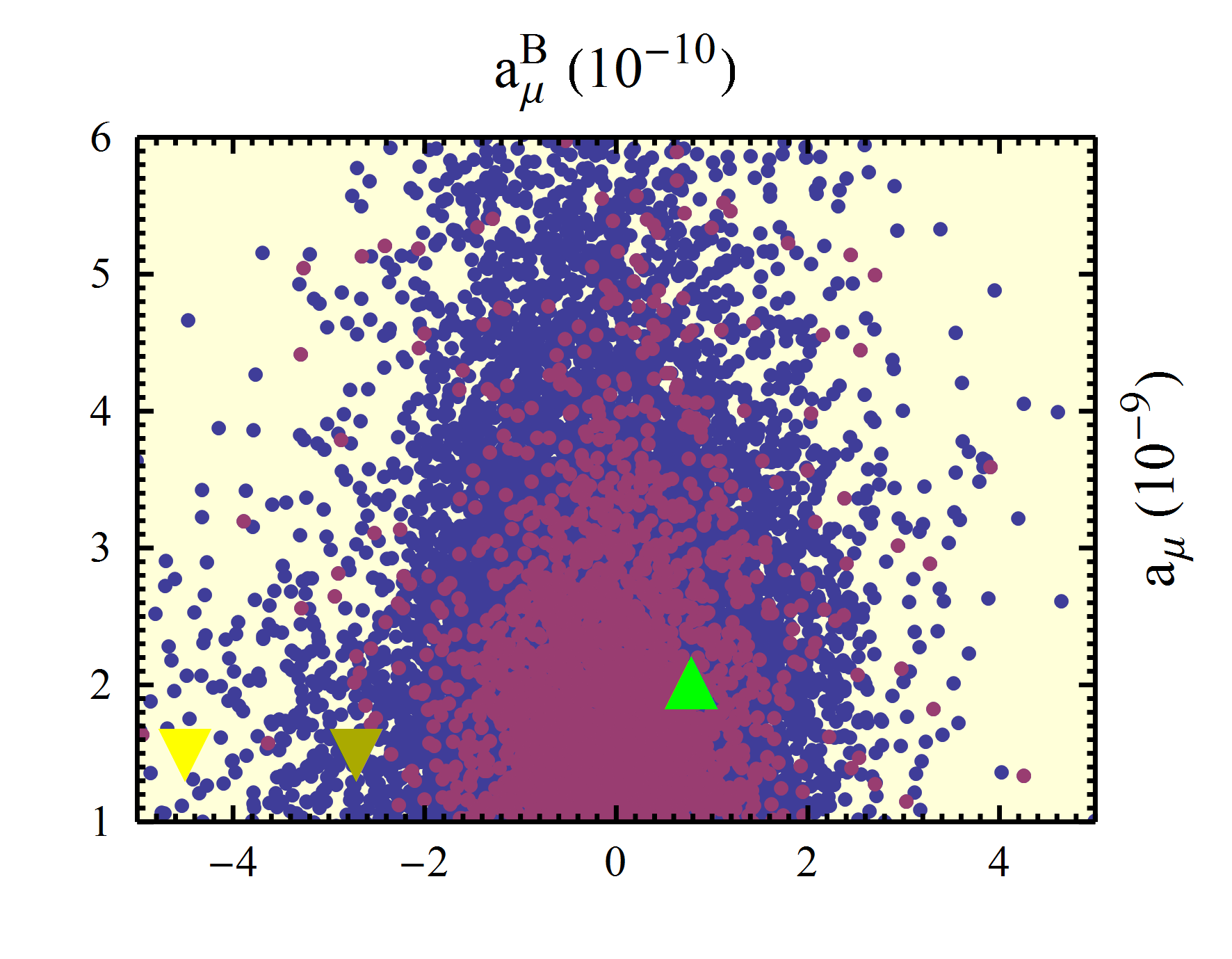
(b) $\eta=0.1$

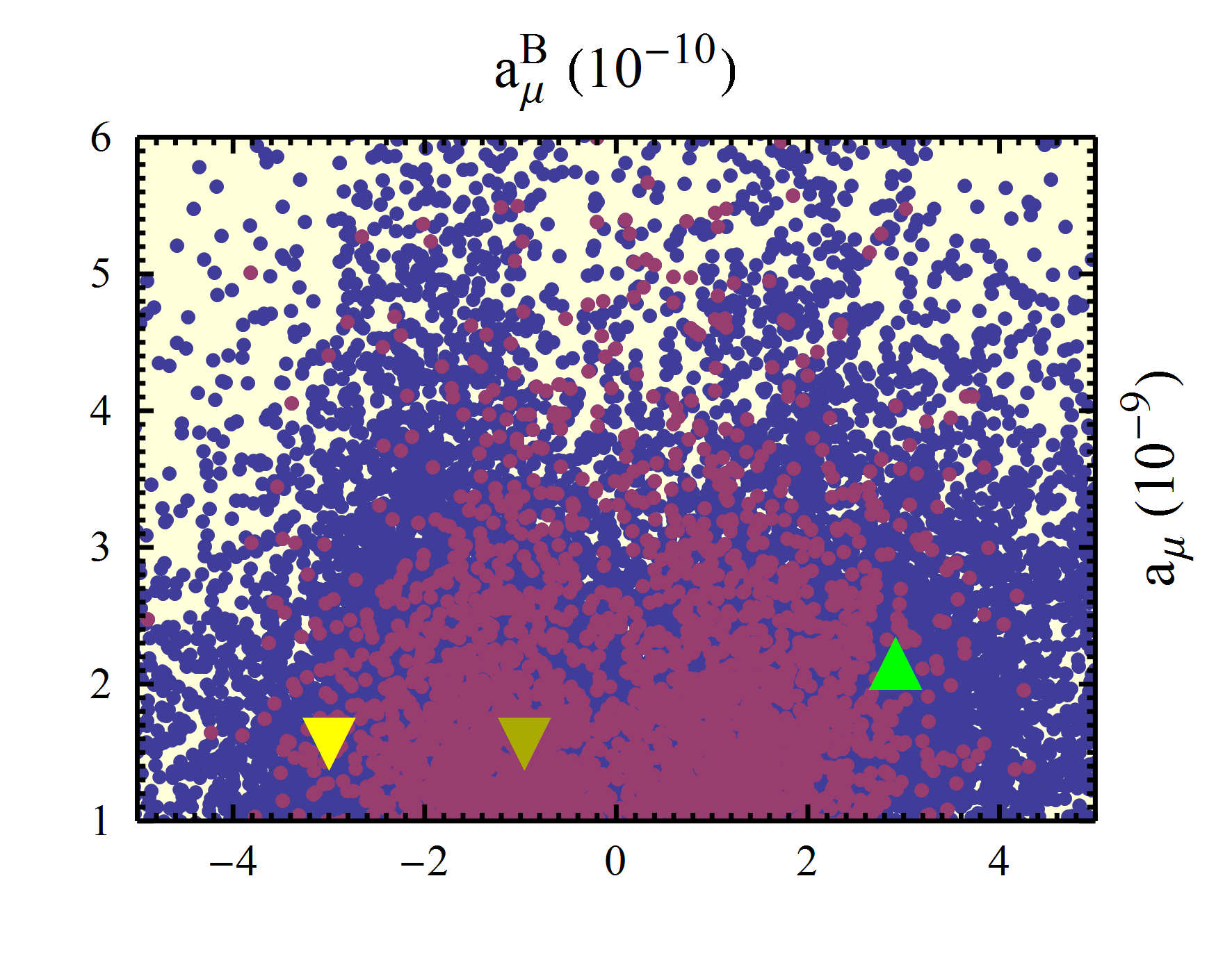
(c) $\eta=-0.1$

Figure 9: Scatter plots showing possible values for $a_{\mu}$ and $a_{\mu}^{\text{B}}$ evaluated at different $\eta$ values. Blue dots represent points in the general allowed parameter space Eq. (65) while red dots represent the remaining ones after the constraints are applied. Green and yellow triangles are representative points discussed in the text.

Since we want to study the impact of the SM-limit deviation to $a_{\mu}$, hereafter we will choose specific values for $\eta$ and compare how the results differ.

We perform a scan over the above region, computing for each point the value of the full $a_{\mu}$ as well the contribution only due to two-loop bosonic Feynman diagrams. Our results of the full scan are depicted as blue points in the plots of Fig. 9 (for the three values $\eta=0$, $\eta=0.1$, $\eta=-0.1$). We then apply the further experimental/theoretical constraints discussed in Sec. 2.2. The survival sample is depicted as red points in Fig. 9.

As can be readily seen, although the values for the full $a_{\mu}$ can be large, the contribution from $a_{\mu}^{\text{B}}$ can amount to $(2\cdots 4)\times 10^{-10}$. One can also notice a difference in behavior between the SM-limit case and the one in which $\eta$ is negative. In the latter case, one observes that the range of values for $a_{\mu}^{\text{B}}$ is significantly larger, spreading over the x-axis, while in the former it is constrained inside the region with absolute value $2\times 10^{-10}$.

In order to obtain a better insight into the bosonic contribution, we choose a sample point for which the muon anomaly can be explained and vary the parameters affecting mainly $a_{\mu}^{\text{B}}$. For comparison with the previous analysis [28], we consider as starting value a parameter space point allowed by the type X model.

In the type X model, the explanation to the $a_{\mu}$ deviation comes mainly from fermionic contributions containing a tau loop. The reason is that, in this model, only the Yukawa coupling of leptons is enhanced, see Table 1. In the Aligned Model, a type X scenario is recovered if $\zeta_{u}=\zeta_{d}=1/t_{\beta}$, and $\zeta_{l}$ is identified as $-t_{\beta}$. In Ref. [28], it was found that the anomaly could be explained for low values of the CP-odd scalar mass ($M_{A}<100\;\text{GeV}$), large $t_{\beta}$, and values of the masses of the CP-even and charged scalar of the order of $200\;\text{GeV}$. In that reference, the type X model was considered and only fermionic contributions were included. Therefore, it is particularly simple to translate parameter points to the Aligned 2HDM, by identifying $t_{\beta}$ as $-\zeta_{l}$. After these considerations, we choose as representative point the one defined by

$$M_{A}=50\;\text{GeV},\quad M_{H}=M_{H^{\pm}}=200\;\text{GeV},\quad\zeta_{l}=-100,\quad\zeta_{u}=\zeta_{d}=0.01.$$ (66)

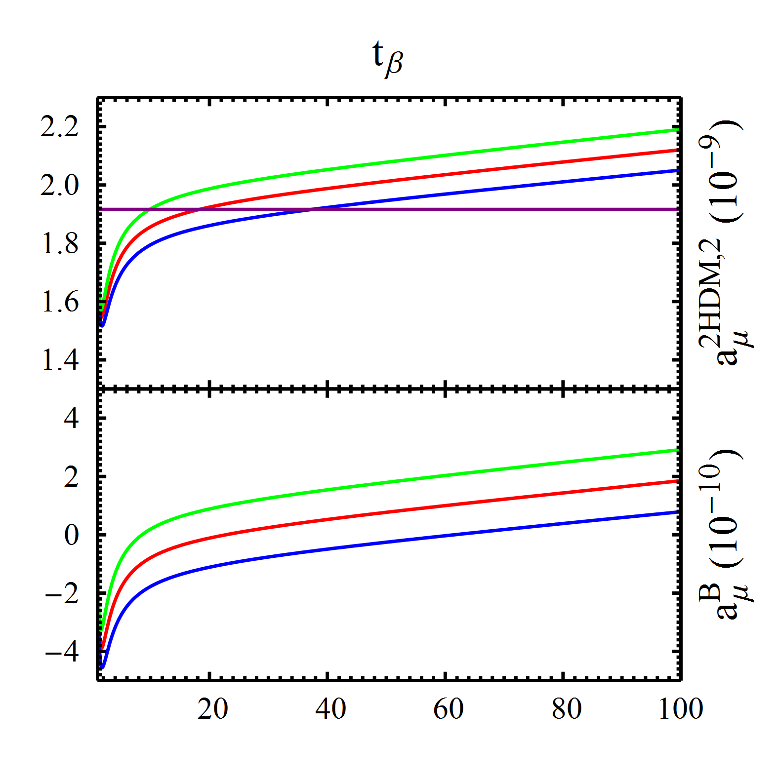
(a)

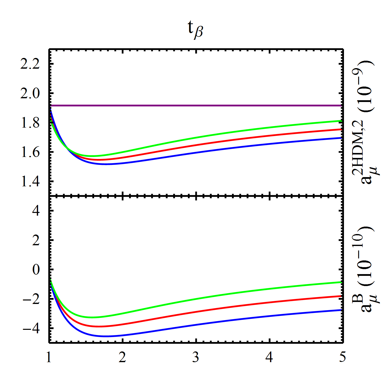
(b)

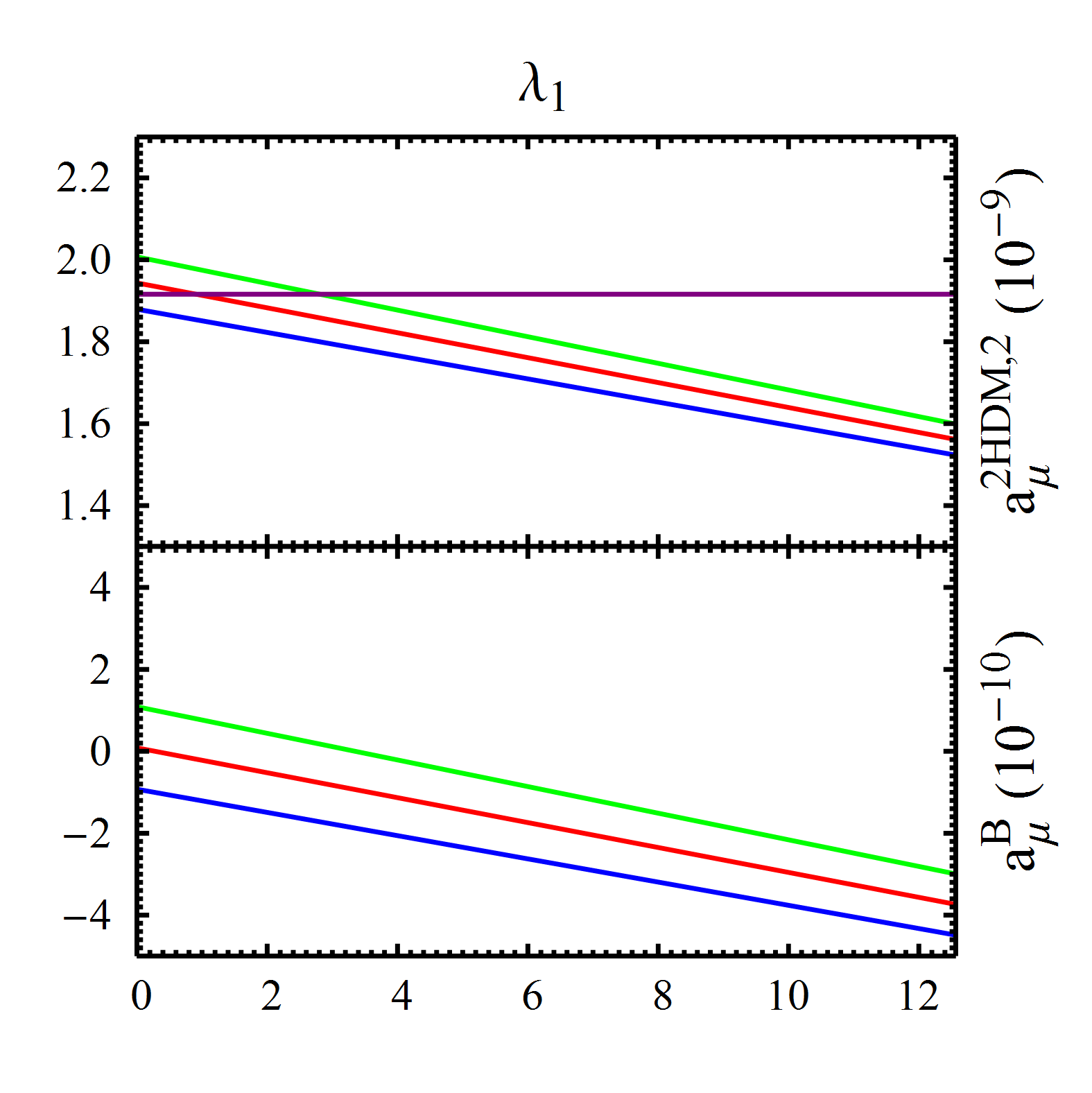
(c)

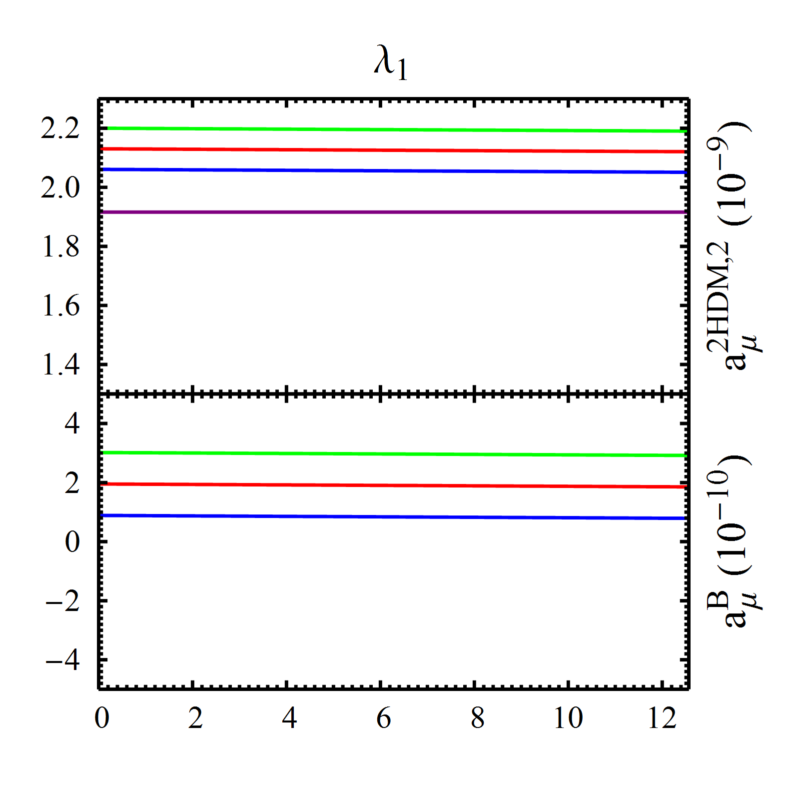
(d)

Figure 10: Plots showing the behavior of $a_{\mu}^{{\text{2HDM}},2}$, and $a_{\mu}^{\text{B}}$. Each red/blue/green line is for $\eta=0/0.1/-0.1$. $t_{\beta}$ varies for (a) and (b), and $\lambda_{1}$ for (c) and (d). We consider the representative mass parameter point in Eq. (66). $\lambda_{1}=4\pi$ for (a) and (b). We employ $t_{\beta}=2$ and $t_{\beta}=100$ for (c) and (d) respectively.

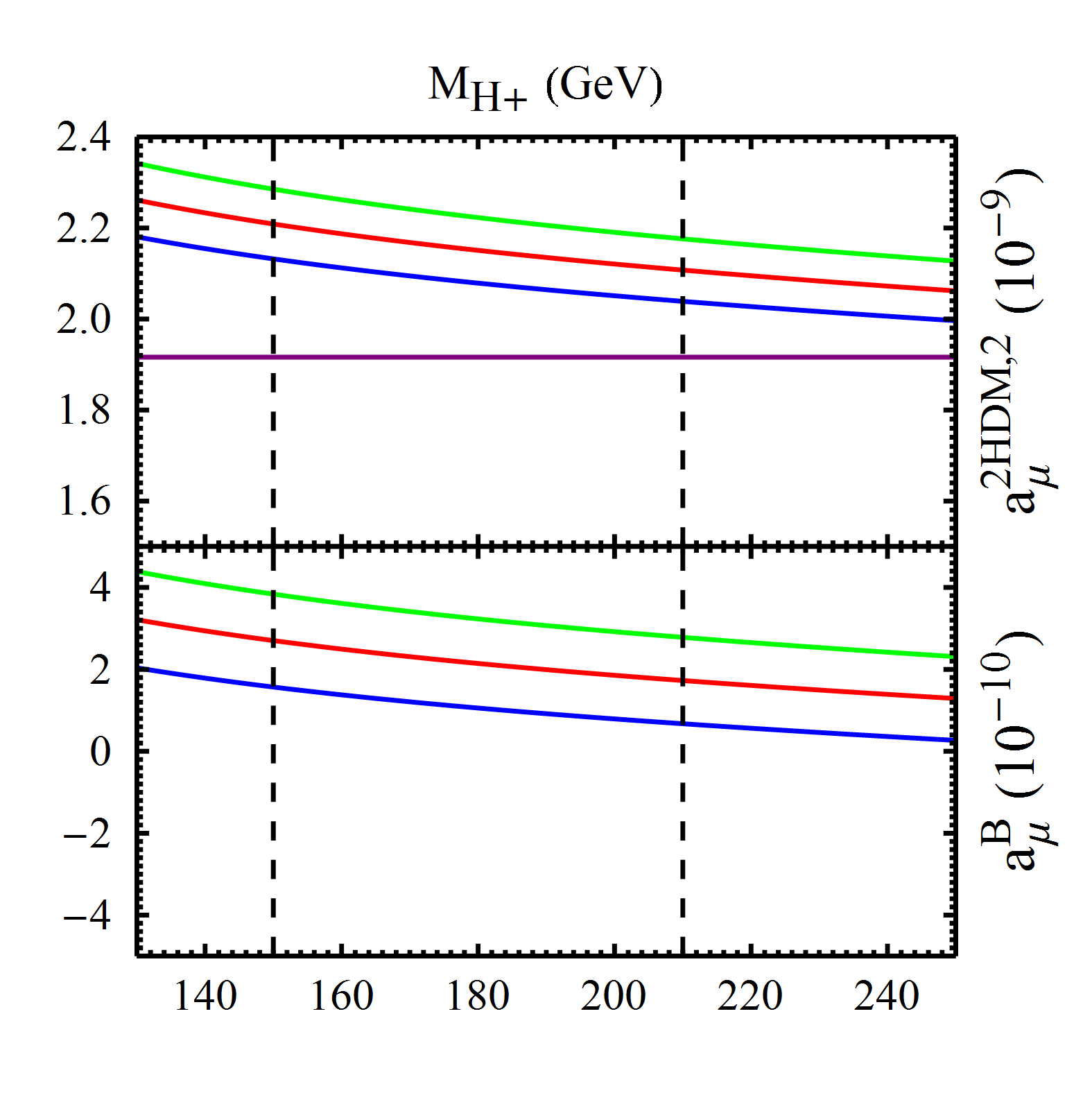
(a)

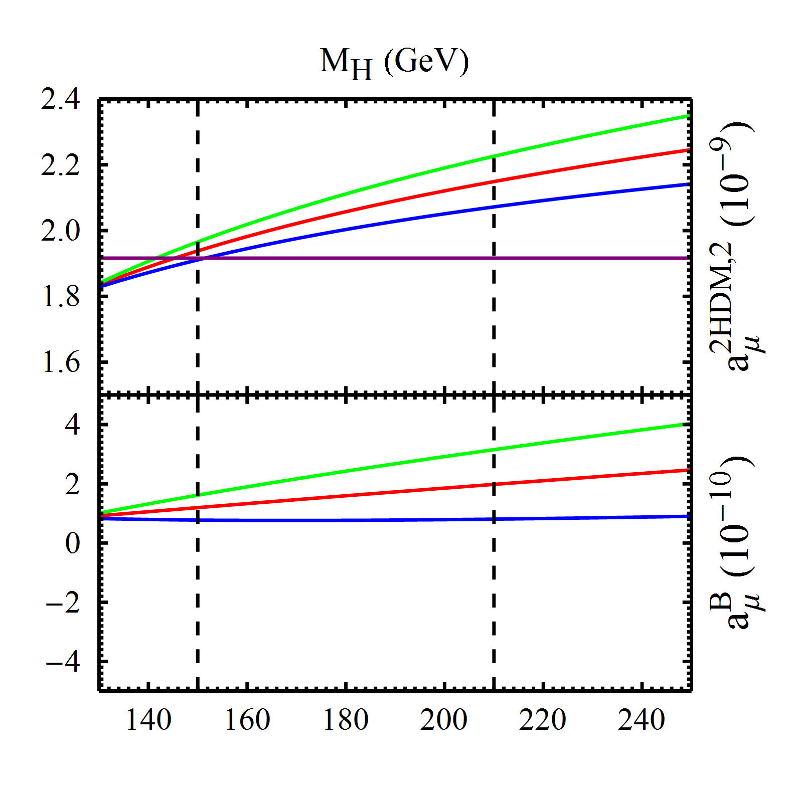
(b)

Figure 11: Plots showing the behavior of $a_{\mu}^{{\text{2HDM}},2}$, and $a_{\mu}^{\text{B}}$. Each red/blue/green line is for $\eta=0/0.1/-0.1$. $M_{H^{\pm}}$ and $M_{H}$ vary in (a) and (b) respectively. We set $\lambda_{1}=4\pi$, and $t_{\beta}=100$. The inside regions between the dashed lines are allowed by constraints. The purple line is a reference value as explained in the text.

In the Aligned model, the values for $t_{\beta}$, $\lambda_{1}$, and $\eta$ remain free. The first two are only related to the bosonic contribution via triple Higgs couplings, $\eta$ affects the bosonic and fermionic contributions. Fig. 13 shows the results from varying these three parameters, and thus particularly the impact of the bosonic contribution to $a_{\mu}$. In all plots we depict $a_{\mu}^{{\text{2HDM}},2}$ on the upper graph, and $a_{\mu}^{\text{B}}$ on the lower one. The upper plots contain as a reference line the value for $a_{\mu}$ used in [28], which takes into account only fermionic contributions for $\eta=0$. The $\eta$-dependence is depicted by red lines ($\eta=0$), blue lines ($\eta=0.1$), and green lines ($\eta=-0.1$). We proceed to explain each of the graphs individually.

Figs. 13(a) – 13(b) show the behavior as a function of $t_{\beta}$ for $\lambda_{1}=4\pi$. As expected from the scatter plots, the variation of $a_{\mu}^{\text{B}}$ is in the range $(2\cdots 4)\times 10^{-10}$, and the contribution can either be negative or positive. The behavior can be understood by analyzing the formula for $\Lambda_{5}$, Eq. (15), the general formula for $a_{\mu}^{\text{B}}$, Eq. (48), and the values of the different coefficients, Figs. 4 – 6.

There are two regions: small $t_{\beta}$ and large $t_{\beta}$. For small $t_{\beta}$, $\Lambda_{5}$ is dominated by the negative term proportional to $\lambda_{1}$ and several bosonic contributions are suppressed by $(t_{\beta}-1/t_{\beta})$ which vanishes as $t_{\beta}\rightarrow 1$. This explains the linear behavior in Fig. 13(c) and the peak in Fig. 13(b).

For large $t_{\beta}$, $\Lambda_{5}\simeq 2M_{H}^{2}/v^{2}\simeq 1.32$, and the prefactor $(t_{\beta}-1/t_{\beta})\simeq t_{\beta}$. This explains the linear behavior of the contributions for $t_{\beta}>20$ in Fig. 13(a) and the independence of $\lambda_{1}$ in Fig. 13(d).

Regarding the $\eta$-dependence, the dominant terms depending on $\eta$ are $a_{\mu}^{\text{EW add.}}$, Eq. (49), and $a_{0,z}^{1}$, Fig. 6(b). For the present parameter region, the coefficients of $\eta\,\zeta_{l}$ are approximately $(2.3-1)\times 10^{-11}$. This explains that shifting $\eta$ by $0.1$ decreases $a_{\mu}^{\text{B}}$ by $10^{-10}$ in all plots.

In order to compare our analysis of Fig. 13 with the scatter plots of Fig. 9, we show three representative points in Fig. 9. The first, in green, is the representative point just discussed for the large $t_{\beta}$ regime ($t_{\beta}=100$, $\lambda_{1}$ arbitrary). The other two, yellow and dark yellow, are related to the low $t_{\beta}$ regime and have $t_{\beta}=2$ and two different values of $\lambda_{1}$, $\lambda_{1}=4\pi$ (yellow) and $\lambda_{1}=2\pi$ (dark yellow). As can be seen, the green triangle for $\eta=-0.1$ and $\eta=0$ is close to the border of the constrained sample depicted in red while, for $\eta=0.1$, the green triangle is well inside the allowed area. It is instructive to notice that, for negative values of $\eta$, there is a considerable sample of allowed points with similar values for $a_{\mu}^{\text{B}}\simeq(2\cdots 3)\times 10^{-10}$. This behavior is explained by observing Figs. 13(a) – 13(d) which show that for any value of $\lambda_{1}$ there is a large interval for $t_{\beta}$, $40<t_{\beta}<100$, allowing $a_{\mu}^{\text{B}}>2\times 10^{-10}$. This situation should be contrasted with the low $t_{\beta}$ regime, represented by the yellow triangles. While the $\eta=-0.1$ case still has a considerable amount of points with similar values, the ($\eta=0,\;0.1$) cases represent rare points in the constrained sample for $\lambda_{1}=4\pi$, and points close to the border of the allowed area for $\lambda_{1}=2\pi$. The explanation can be found in Figs. 13(b) – 13(c) which show that values for $a_{\mu}^{\text{B}}$ similar to the ones of the light yellow triangle can only be obtained for a small range of $t_{\beta}$, $1<t_{\beta}<5$, and large values of $\lambda_{1}$, $\lambda_{1}\simeq 4\pi$. These observations explain why the scatter plot for negative $\eta$, Fig. 9(c), has more allowed points with values for $|a_{\mu}^{\text{B}}|$ of order $(2\cdots 4)\times 10^{-10}$ if compared with the other cases.

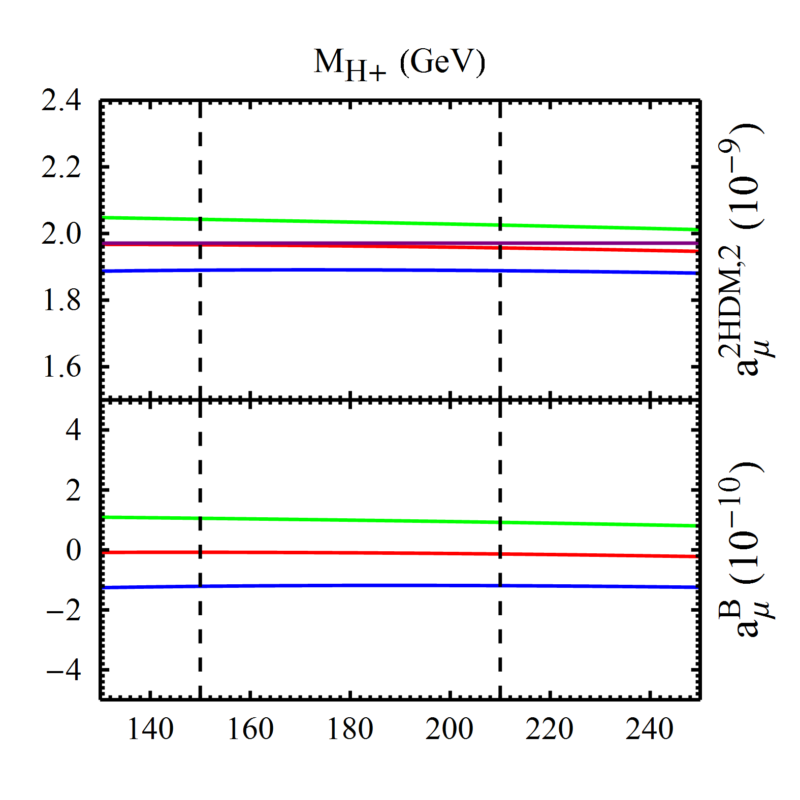
(a)

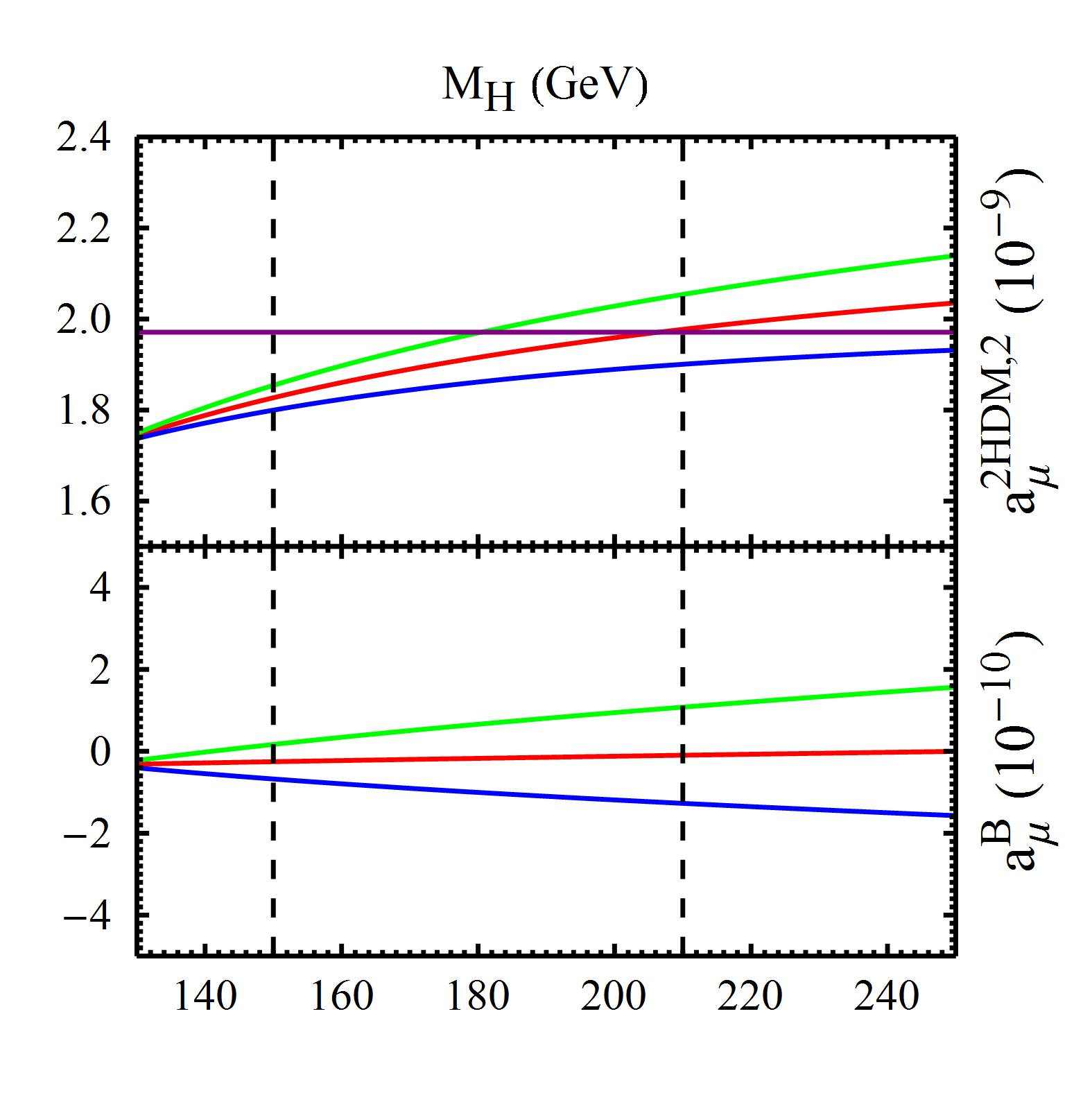
(b)

Figure 14: Revised version of figure 11. Plots showing the behavior of $a_{\mu}^{{\text{2HDM}},2}$, and $a_{\mu}^{\text{B}}$. Each red/blue/green line is for $\eta=0/0.1/-0.1$. $M_{H^{\pm}}$ and $M_{H}$ vary in (a) and (b) respectively. We set $\lambda_{1}=4\pi$, and $t_{\beta}=100$. The inside regions between the dashed lines are allowed by constraints. The purple line is a reference value as explained in the text.

Finally we discuss the plots of Fig. 14. In both cases we study the behavior of $a_{\mu}^{{\text{2HDM}},2}$ and $a_{\mu}^{\text{B}}$ as functions of one of the masses of the scalars ($M_{H^{\pm}}$, and $M_{H}$ respectively) where the region delimited by the dashed lines is allowed by theoretical and EW constraints. The other mass and aligned parameters are kept fixed as in the representative point Eq. (66). Regarding $t_{\beta}$, we choose $t_{\beta}=100$, corresponding to a type X parameter point. Since we are in the large $t_{\beta}$ limit, $\lambda_{1}$ has no significant influence. We adopt $\lambda_{1}=4\pi$. As can be seen in Fig. 14(a), there is a slight mass dependence in $a_{\mu}^{{\text{2HDM}},2}$. To illustrate the mass dependence we first remark that, for the parameter region we are considering, only the coefficients enhanced by $\zeta_{l}$ and $t_{\beta}$ are important, namely $a_{0,z}^{0}$ and $a_{5,z}^{0}$. Using the definitions in Appendix A and considering the large $t_{\beta}$ region, one has

$$a_{\mu}^{\text{B}}|_{\eta=0}\simeq (a_{0,z}^{0}+\Lambda_{5}a_{5,z}^{0})\zeta_{l}t_{\beta}$$

$$= \left[-b(x_{H},0)-\frac{\Lambda_{5}}{2}\right]\left[{\mathcal{F}}_{m}^{0}(x_{H},x_{H^{\pm}})+{\mathcal{F}}_{m}^{\pm}(x_{H},x_{H^{\pm}})\right]\zeta_{l}t_{\beta}$$

$$\simeq -6.3\times 10^{-7}M_{H}^{2}\left[{\mathcal{F}}_{m}^{0}(x_{H},x_{H^{\pm}})+{\mathcal{F}}_{m}^{\pm}(x_{H},x_{H^{\pm}})\right]\zeta_{l}t_{\beta},$$ (67)

where $x_{\cal S}\equiv M_{\cal S}^{2}/M_{Z}^{2}$, and we used $\Lambda_{5}\simeq 2M_{H}^{2}/v^{2}$. The term containing the functions ${\mathcal{F}}_{m}^{0}$, ${\mathcal{F}}_{m}^{\pm}$ is always positive and depends on the inverse of the scalar masses.

Therefore, if $M_{H}$ is kept fixed and $M_{H^{\pm}}$ increases, $|a_{\mu}^{\text{B}}|$ will decrease, explaining the behavior observed in Fig. 14(a). In contrast, if $M_{H^{\pm}}$ is kept fixed and $M_{H}$ increases, the explicit dependency on $M_{H}^{2}$ coming from $\Lambda_{5}$ and the coefficient $b(x_{H},0)$ leads to an increase of $a_{\mu}^{\text{B}}$ with $M_{H}$ in Fig. 14(b).

Regarding the full $a_{\mu}$, we verified that the fermionic contributions essentially do not depend on $M_{H^{\pm}}$ due to the small $\zeta_{u}$, but they depend on $M_{H}$. As can be noticed analyzing the plots of Fig. 8 and Table 3, the fermionic contributions from $H$ diagrams are negative and decrease in modulus with $M_{H}$. Therefore, the net result will be an increase in $a_{\mu}$ as observed in Fig. 14(b).

Finally, it can also be noticed that the plots for non-zero values of $\eta$ tend to the case $\eta=0$ as $M_{H}$ approaches $M_{h}$. This behavior can be understood by observing that in this case the two mass-degenerate CP-even scalars together behave exactly SM-like.

5 Conclusion

We presented the full two-loop 2HDM contributions to $a_{\mu}$, providing the complete analytic result and a numerical analysis. We confirmed the previous results of the fermion-loop and the bosonic Barr-Zee type contributions. We calculated the remaining diagrams including all 3-boson diagrams, which involve three internal boson couplings to the muon line.

The analytic results are expressed in terms of physical parameters. The full bosonic result depends on the three additional Higgs boson masses, $t_{\beta}$, $\sin\alpha$, the alignment parameter $\zeta_{l}$ and the quartic scalar coupling $\lambda_{1}$. We always expand in the small parameter $\eta=\alpha-\beta+\pi/2$, the deviation from the SM-limit. The bosonic contributions are especially dependent on $t_{\beta}$ and $\lambda_{1}$, whereas fermionic ones are not. This dependency arises from the triple Higgs couplings in the bosonic Feynman diagrams.

We split the bosonic result into several parts, see Eq. (48) and Eq. (• ‣ 3.3.2). Each term has a straightforward dependence on $t_{\beta}$ and $\zeta_{l}$ and depends only on a subset of masses. The compact analytic expression of each term is provided in Appendix A. We documented the parameter dependence in a series of Figures in Sec. 3.3.

We also confirmed the previous result of the fermionic contribution. Particularly, we presented its analytic form without one-dimensional integral relations in Sec. 3.4 and gave an overview of the numerical behavior. The fermionic result involves all three alignment parameters $\zeta_{l,u,d}$, but the leading contributions are the $\zeta_{l}$ dependent terms.

We also investigated the impact of the scenario with a deviation from the SM-limit of the Higgs couplings, $\eta=\alpha-\beta+\pi/2\neq 0$. For this case, we obtain additional contributions from the SM-like Higgs boson, $a_{\mu}^{\text{EW add.}}$. This term is proportional to $\eta\,\zeta_{l}$ and gives the dominant $\eta$-dependent bosonic contributions. Its coefficient is dependent only on the SM parameters and can be found in Eq. (49).

In the numerical evaluation we confirmed that the fermionic 2HDM contribution can be of the order of the deviation Eq. (1). A series of plots shows that in parameter regions with large fermionic contributions, the complete bosonic result can yield additional contributions in the range $(2\cdots 4)\times 10^{-10}$, i.e. at the level of the precision of the planned Fermilab experiment. Allowing the SM-like Higgs couplings to deviate from the SM-limit, i.e. $\eta\neq 0$, and non-zero values of $\lambda_{1}$, can slightly increase the bosonic contributions.

Appendix A Analytic results

Here we provide the full analytic result of the complete renormalized bosonic two-loop contributions $a_{\mu}^{\text{B}}$, in the decomposition of Eq. (48). We begin with required loop function (defined first in Ref. [76]):

$${\Phi}(m_{1},m_{2},m_{3}) =\frac{\lambda}{2}\Bigg{[}2\ln(\alpha_{+})\ln(\alpha_{-})-\ln\left(\frac{m_{1}^{2}}{m_{3}^{2}}\right)\ln\left(\frac{m_{2}^{2}}{m_{3}^{2}}\right)$$

$$-2\text{Li}_{2}(\alpha_{+})-2\text{Li}_{2}(\alpha_{-})+\frac{\pi^{2}}{3}\Bigg{]},$$ (68)

$$\lambda =\sqrt{m_{1}^{4}+m_{2}^{4}+m_{3}^{4}-2m_{1}^{2}m_{2}^{2}-2m_{2}^{2}m_{3}^{2}-2m_{3}^{2}m_{1}^{2}}\;,$$ (69)

$$\alpha_{\pm} =\frac{m_{3}^{2}\pm m_{1}^{2}\mp m_{2}^{2}-\lambda}{2m_{3}^{2}}.$$ (70)

The coefficient $a_{\mu}^{\text{non-Yuk}}$ of the contribution without Yukawa couplings is given by

$$a_{\mu}^{\text{non-Yuk}}= \frac{\alpha^{2}}{576\,\pi^{2}\,c_{\text{W}}^{4}s_{\text{W}}^{4}}\,\frac{m_{\mu}^{2}}{M_{Z}^{2}}\,\left\{\left(\frac{x_{A}-x_{H}}{x_{A}-x_{H^{\pm}}}\right){\mathcal{T}}_{2}^{+}(x_{A},x_{H})+{\mathcal{T}}_{2}^{-}(x_{H},x_{H^{\pm}})\right.$$

$$+\left(\frac{x_{A}-x_{H}}{x_{A}-x_{H^{\pm}}}\right){\mathcal{T}}_{4}(x_{A},x_{H^{\pm}})+{\mathcal{T}}_{4}(x_{H},x_{A})+{\mathcal{T}}_{5}(x_{H^{\pm}},x_{H})+{\mathcal{T}}_{5}(x_{H^{\pm}},x_{A})$$

$$+{\mathcal{T}}_{2}^{+}(x_{H^{\pm}},x_{H})+{\mathcal{T}}_{2}^{+}(x_{H^{\pm}},x_{A})+{\mathcal{T}}_{6}(x_{A},x_{H^{\pm}})+{\mathcal{T}}_{6}(x_{H},x_{H^{\pm}})$$

$$+{\mathcal{T}}_{7}(x_{A},x_{H})+{\mathcal{T}}_{7}(x_{H^{\pm}},x_{H^{\pm}})(1-2c_{\text{W}}^{2})^{2}+{\mathcal{T}}_{8}(x_{A},x_{H^{\pm}})+{\mathcal{T}}_{8}(x_{H},x_{H^{\pm}})$$

$$-\frac{16}{3}c_{\text{W}}^{2}s_{\text{W}}^{2}(1+8c_{\text{W}}^{2}-8c_{\text{W}}^{4})+\frac{8c_{\text{W}}^{4}s_{\text{W}}^{4}}{5x_{H^{\pm}}}+f_{2}x_{H^{\pm}}-f_{3}x_{H^{\pm}}^{2}$$

$$+f_{1}(x_{A}^{2}+x_{H}^{2})+f_{3}x_{H^{\pm}}(x_{A}+x_{H})+f_{4}(x_{A}+x_{H})-f_{5}x_{A}x_{H}$$

$$\left.+{\mathcal{T}}_{1}(x_{A},x_{H^{\pm}})+{\mathcal{T}}_{1}(x_{H},x_{H^{\pm}})+{\mathcal{T}}_{0}(x_{A},x_{H^{\pm}})+{\mathcal{T}}_{0}(x_{H},x_{H^{\pm}})\right\}.$$ (71)

The abbreviations appearing in $a_{\mu}^{\text{non-Yuk}}$ are

$${\mathcal{T}}_{0}(u,\omega)= \frac{9}{c_{\text{W}}^{4}}\frac{(u-\omega)(c_{\text{W}}^{2}(u-\omega)(u+2\omega)-(u-\omega)^{3}+c_{\text{W}}^{4}\omega)}{c_{\text{W}}^{4}+(u-\omega)^{2}-2c_{\text{W}}^{2}(u+\omega)}$$

$$\times{\Phi}(\sqrt{u},\sqrt{\omega},c_{\text{W}}),$$ (72)

$${\mathcal{T}}_{1}(u,\omega)= \frac{9}{c_{\text{W}}^{4}}(u-\omega)(c_{\text{W}}^{2}\omega-(u-\omega)^{2})\text{Li}_{2}(1-u/\omega),$$ (73)

$${\mathcal{T}}_{2}^{\pm}(u,\omega)= \ln(u)\left(\frac{6u^{2}+c_{\text{W}}^{2}(u-x_{H^{\pm}})+2c_{\text{W}}^{4}(u-x_{H^{\pm}})}{2(u-\omega)}\right.$$

$$+f_{6}\frac{(u-x_{H^{\pm}})^{2}(3c_{\text{W}}^{4}+3c_{\text{W}}^{2}(u-x_{H^{\pm}})+(u-x_{H^{\pm}})^{2}}{c_{\text{W}}^{2}(u-\omega)}$$

$$\pm f_{7}\frac{3u^{2}(u-x_{H^{\pm}})}{(x_{A}-x_{H})(u-\omega)}-f_{8}\frac{3u(u-x_{H^{\pm}})^{2}}{2(u-\omega)}$$

$$-\left.f_{9}\frac{3u(u-x_{H^{\pm}})}{2(u-\omega)}\right),$$ (74)

$${\mathcal{T}}_{4}(u,\omega)= \frac{(u-\omega)\ln(u)}{4}f_{5}(x_{A}(3+2x_{H})-x_{A}^{2}+3x_{H}-x_{H}^{2}-3),$$ (75)

$${\mathcal{T}}_{5}(u,\omega)= \ln(u)\left(\frac{3}{2}u+\frac{f_{6}}{c_{\text{W}}^{2}}((u-\omega)^{3}+3c_{\text{W}}^{2}(u-\omega)^{2}+3c_{\text{W}}^{4}(u-\omega))\right.$$

$$\left.-\frac{3}{2}f_{8}u(u-\omega)-\frac{c_{\text{W}}^{2}}{2}-c_{\text{W}}^{4}\right),$$ (76)

$${\mathcal{T}}_{6}(u,\omega)= \frac{9}{2}\left(\frac{(u-\omega)(u^{2}-2u\omega+\omega(\omega-c_{\text{W}}^{2}))}{c_{\text{W}}^{4}}\ln\left(\frac{u}{\omega}\right)\ln\left(\frac{\omega}{c_{\text{W}}^{2}}\right)\right.$$

$$\left.+\frac{\ln(c_{\text{W}}^{2})}{c_{\text{W}}^{2}}(2u^{2}+u(c_{\text{W}}^{2}-4\omega)-\omega(c_{\text{W}}^{2}-2\omega))\right),$$ (77)

$${\mathcal{T}}_{7}(u,\omega)= -\frac{f_{5}}{2}(2(u+\omega)-(u-\omega)^{2}-1)\ln\left(\frac{{\mathcal{S}}_{1}(u,\omega)}{2\sqrt{u\omega}}\right)$$

$$\times\left(u+\omega-1-\frac{4u\omega}{{\mathcal{S}}_{1}(u,\omega)}\right),$$ (78)

$${\mathcal{S}}_{1}(u,\omega)= u+\omega-1+\sqrt{1+(u-\omega)^{2}-2(u+\omega)},$$ (79)

$${\mathcal{T}}_{8}(u,\omega)= 2f_{6}(4u\omega-(u+\omega-c_{\text{W}}^{2})^{2})\ln\left(\frac{{\mathcal{S}}_{2}(u,\omega)}{2\sqrt{u\omega}}\right)$$

$$\times\left(\frac{(u+\omega)}{c_{\text{W}}^{2}}-\frac{4u\omega}{c_{\text{W}}^{2}{\mathcal{S}}_{2}(u,\omega)}-1\right),$$ (80)

$${\mathcal{S}}_{2}(u,\omega)= u+\omega-c_{\text{W}}^{2}+\sqrt{(u+\omega-c_{\text{W}}^{2})^{2}-4u\omega}.$$ (81)

The following coefficients depend only on known SM parameters; we provide therefore also approximate numerical values:

$$f_{1}= \frac{7}{2}-\frac{25}{2c_{\text{W}}^{2}}+4c_{\text{W}}^{2}-4c_{\text{W}}^{4} = -12,$$ (82)

$$f_{2}= 2(17-24c_{\text{W}}^{2}+56c_{\text{W}}^{4}-128c_{\text{W}}^{6}+64c_{\text{W}}^{8}) = -9.1,$$ (83)

$$f_{3}= \frac{25-32c_{\text{W}}^{2}+4c_{\text{W}}^{4}}{c_{\text{W}}^{2}s_{\text{W}}^{2}} = 15,$$ (84)

$$f_{4}= \frac{13}{2}-15c_{\text{W}}^{2}+10c_{\text{W}}^{4} = -0.9,$$ (85)

$$f_{5}= \frac{c_{\text{W}}^{2}(5-16c_{\text{W}}^{2}+8c_{\text{W}}^{4})}{s_{\text{W}}^{2}} = -9,$$ (86)

$$f_{6}= \frac{7-14c_{\text{W}}^{2}+4c_{\text{W}}^{4}}{4c_{\text{W}}^{2}s_{\text{W}}^{2}} = -2,$$ (87)

$$f_{7}= 1-6c_{\text{W}}^{2}+4c_{\text{W}}^{4} = -1.2,$$ (88)

$$f_{8}= \frac{13-20c_{\text{W}}^{2}+4c_{\text{W}}^{4}}{c_{\text{W}}^{2}s_{\text{W}}^{2}} = -0.7,$$ (89)

$$f_{9}= 7-12c_{\text{W}}^{2}+8c_{\text{W}}^{4} = 2.5.$$ (90)

The coefficients of the Yukawa-dependent terms in Eq. (• ‣ 3.3.2) are given by

$$a_{0,0}^{0} =b(x_{H_{\text{SM}}},x_{H^{\pm}}){\mathcal{F}}_{m}^{0}(x_{H_{\text{SM}}},x_{H^{\pm}});$$ (91)

$$a_{0,z}^{0} =-b(x_{H},0)\left[{\mathcal{F}}_{m}^{0}(x_{H},x_{H^{\pm}})+{\mathcal{F}}_{m}^{\pm}(x_{H},x_{H^{\pm}})\right];$$ (92)

$$a_{5,0}^{0} ={\mathcal{F}}_{m}^{0}(x_{H_{\text{SM}}},x_{H^{\pm}});$$ (93)

$$a_{5,z}^{0} =-\frac{1}{2}\left[{\mathcal{F}}_{m}^{0}(x_{H},x_{H^{\pm}})+{\mathcal{F}}_{m}^{\pm}(x_{H},x_{H^{\pm}})\right];$$ (94)

$$a_{0,0}^{1} =b(x_{H},0){\mathcal{F}}_{m}^{0}(x_{H},x_{H^{\pm}})-(x_{H}\rightarrow x_{H_{\text{SM}}});$$ (95)

$$a_{0,z}^{1} =-\bigg{[}b(x_{H},x_{H^{\pm}})\left({\mathcal{F}}_{m}^{0}(x_{H},x_{H^{\pm}})+{\mathcal{F}}_{m}^{\pm}(x_{H},x_{H^{\pm}})\right)$$

$$\quad-{\mathcal{F}}_{3}(x_{H},x_{H^{\pm}})-(x_{H}\rightarrow x_{H_{\text{SM}}})\bigg{]}+{\mathcal{F}}_{2}(x_{H});$$ (96)

$$a_{5,0}^{1} =\frac{{\mathcal{F}}_{m}^{0}(x_{H},x_{H^{\pm}})}{2}-(x_{H}\rightarrow x_{H_{\text{SM}}});$$ (97)

$$a_{5,z}^{1} =-{\mathcal{F}}_{m}^{0}(x_{H},x_{H^{\pm}})-{\mathcal{F}}_{m}^{\pm}(x_{H},x_{H^{\pm}})-(x_{H}\rightarrow x_{H_{\text{SM}}}).$$ (98)

The appearing abbreviations are given by

$$b(u,\omega)= \frac{\alpha\pi}{c_{\text{W}}^{2}(-1+c_{\text{W}}^{2})}(u+2\omega),$$ (99)

$${\mathcal{F}}_{m}^{0}(u,\omega)= \frac{\alpha^{2}}{576\,\pi^{2}\,c_{\text{W}}^{4}s_{\text{W}}^{4}}\,\frac{m_{\mu}^{2}}{M_{Z}^{2}}\,\left(\frac{1}{\alpha\pi}\frac{c_{\text{W}}^{2}(-1+c_{\text{W}}^{2})}{(u+2\omega)}\right){\mathcal{F}}_{1}(u,\omega),$$ (100)

$${\mathcal{F}}_{m}^{\pm}(u,\omega)= \frac{\alpha^{2}}{576\,\pi^{2}\,c_{\text{W}}^{4}s_{\text{W}}^{4}}\,\frac{m_{\mu}^{2}}{M_{Z}^{2}}\,\left(-\frac{9(-1+c_{\text{W}}^{2})}{\alpha\pi}\right)\left(\frac{{\mathcal{T}}_{9}(u,\omega)}{2}+{\mathcal{T}}_{10}(u,\omega)\right),$$ (101)

$${\mathcal{F}}_{1}(u,\omega)= -72c_{\text{W}}^{2}(-1+c_{\text{W}}^{2})\frac{u+2\omega}{u}-36c_{\text{W}}^{2}(-1+c_{\text{W}}^{2})\frac{u+2\omega}{u}\ln(\omega)$$

$$+9(-8c_{\text{W}}^{4}-3u+2c_{\text{W}}^{2}(4+u))\frac{(u+2\omega)}{2(u-1)u}\ln(u)$$

$$-9(3-10c_{\text{W}}^{2}+8c_{\text{W}}^{4})\frac{\omega(u+2\omega)}{(4\omega-1)(u-1)}{\Phi}(\sqrt{\omega},\sqrt{\omega},1)$$

$$+9(8c_{\text{W}}^{4}+3u-2c_{\text{W}}^{2}(4+u))\frac{\omega(u+2\omega)}{(4\omega-u)(u-1)u^{2}}{\Phi}(\sqrt{u},\sqrt{\omega},\sqrt{\omega}),$$ (102)

$${\mathcal{T}}_{9}(u,\omega)= -\frac{2\left(c_{\text{W}}^{4}\omega+c_{\text{W}}^{2}\left(u^{2}+u\omega-2\omega^{2}\right)-(u-\omega)^{3}\right){\Phi}\left(\sqrt{u},\sqrt{\omega},c_{\text{W}}\right)}{(c_{\text{W}}^{2}-\omega)\left(c_{\text{W}}^{4}-2c_{\text{W}}^{2}(u+\omega)+(u-\omega)^{2}\right)}$$

$$+\frac{2c_{\text{W}}^{4}\left(u^{2}-4u\omega+2\omega^{2}\right){\Phi}\left(\sqrt{u},\sqrt{\omega},\sqrt{\omega}\right)}{\omega^{2}\left(\omega-c_{\text{W}}^{2}\right)(u-4\omega)}$$

$$-\frac{2\left(c_{\text{W}}^{2}u(u-2\omega)+\omega(u-\omega)^{2}\right)\text{Li}_{2}\left(1-\frac{u}{\omega}\right)}{\omega^{2}},$$ (103)

$${\mathcal{T}}_{10}(u,\omega)= \frac{u^{2}-c_{\text{W}}^{2}\omega-2u\omega+\omega^{2}}{2(c_{\text{W}}^{2}-\omega)}\ln\left(\frac{\omega}{u}\right)\ln\left(\frac{\omega}{c_{\text{W}}^{2}}\right)$$

$$+\frac{c_{\text{W}}^{2}(c_{\text{W}}^{2}+2u-2\omega)}{2(c_{\text{W}}^{2}-\omega)}\ln\left(\frac{\omega}{c_{\text{W}}^{2}}\right)+\frac{c_{\text{W}}^{2}}{\omega}u\ln\left(\frac{\omega}{u}\right)+\frac{c_{\text{W}}^{2}}{\omega}(\omega-u),$$ (104)

$${\mathcal{F}}_{2}(u)= F^{\text{W}}(u)+F^{\text{Z}}(u)+$$

$$+\frac{\alpha^{2}}{576\,\pi^{2}\,c_{\text{W}}^{4}s_{\text{W}}^{4}}\,\frac{m_{\mu}^{2}}{M_{Z}^{2}}\,\Bigg{\{}\frac{8c_{\text{W}}^{6}\pi^{2}}{u^{2}}+\frac{F_{0}}{u}+\frac{393c_{\text{W}}^{2}}{8}$$

$$+\left(\frac{F_{1}}{u}+F_{2}+F_{3}u\right)\frac{\ln(c_{\text{W}}^{2})}{(4c_{\text{W}}^{2}-1)(4c_{\text{W}}^{2}-u)}$$

$$+\left(\frac{F_{4}}{u}+F_{5}+F_{6}u+F_{7}u^{2}\right)\frac{\ln(u)}{(u-1)(4c_{\text{W}}^{2}-u)}$$

$$-\frac{3}{2}\left(\frac{32c_{\text{W}}^{6}}{u^{2}}+\frac{21c_{\text{W}}^{4}}{u}+15c_{\text{W}}^{2}-35u\right)\text{Li}_{2}\left(1-\frac{u}{c_{\text{W}}^{2}}\right)$$

$$+(F_{8}+F_{9}u)\frac{9c_{\text{W}}^{2}(-3+4c_{\text{W}}^{2})}{2}\frac{{\Phi}\left(c_{\text{W}},c_{\text{W}},1\right)}{(4c_{\text{W}}^{2}-1)^{2}(u-1)}$$

$$+\left[\frac{F_{10}}{u^{2}}+\frac{F_{11}}{u}+F_{12}+F_{13}u+F_{14}u^{2}+\frac{105u^{3}}{2}\right]\frac{{\Phi}\left(\sqrt{u},c_{\text{W}},c_{\text{W}}\right)}{(4c_{\text{W}}^{2}-u)^{2}(u-1)}\Bigg{\}},$$ (105)

$$F_{0}= \frac{3c_{\text{W}}^{4}\left(-640+576c_{\text{W}}^{2}+7\pi^{2}\right)}{4} = -55.9,$$ (106)

$$F_{1}= 96c_{\text{W}}^{6}\left(11-53c_{\text{W}}^{2}+36c_{\text{W}}^{4}\right) = -380,$$ (107)

$$F_{2}= -\frac{3}{4}c_{\text{W}}^{2}\left(-66c_{\text{W}}^{2}-48c_{\text{W}}^{4}+672c_{\text{W}}^{6}\right) = -137,$$ (108)

$$F_{3}= -\frac{3}{4}c_{\text{W}}^{2}\left(109-430c_{\text{W}}^{2}+120c_{\text{W}}^{4}\right) = +88.8,$$ (109)

$$F_{4}= 96c_{\text{W}}^{6}\left(-11+9c_{\text{W}}^{2}\right) = -180,$$ (110)

$$F_{5}= \frac{45c_{\text{W}}^{4}}{2}+192c_{\text{W}}^{6} = +103,$$ (111)

$$F_{6}= \frac{3}{4}c_{\text{W}}^{2}\left(157+90c_{\text{W}}^{2}\right) = +132,$$ (112)

$$F_{7}= -\frac{3}{4}\left(18+61c_{\text{W}}^{2}\right) = -49.0,$$ (113)

$$F_{8}= \left(-7+61c_{\text{W}}^{2}-162c_{\text{W}}^{4}+96c_{\text{W}}^{6}\right) = -12.3,$$ (114)

$$F_{9}= (1-5c_{\text{W}}^{2}+10c_{\text{W}}^{4}) = +3.15,$$ (115)

$$F_{10}= -1728c_{\text{W}}^{8}\left(-1+c_{\text{W}}^{2}\right) = +140,$$ (116)

$$F_{11}= 3c_{\text{W}}^{6}\left(-899+768c_{\text{W}}^{2}\right) = -425,$$ (117)

$$F_{12}= \left(387c_{\text{W}}^{4}-363c_{\text{W}}^{6}\right) = +63.4,$$ (118)

$$F_{13}= \frac{9}{2}c_{\text{W}}^{2}\left(57+106c_{\text{W}}^{2}\right) = +486,$$ (119)

$$F_{14}= -\frac{15}{2}\left(7+45c_{\text{W}}^{2}\right) = -314,$$ (120)

$$F^{\text{Z}}(u)= \frac{\alpha^{2}}{576\,\pi^{2}\,c_{\text{W}}^{4}s_{\text{W}}^{4}}\,\frac{m_{\mu}^{2}}{M_{Z}^{2}}\,\Bigg{\{}Z_{1}u\text{Li}_{2}\left(1-u\right)$$

$$+\frac{Z_{2}}{2u^{2}}\Big{[}6(-4+u)u+\pi^{2}(4+3u)+6u(4+u)\ln(u)$$

$$-6(4+3u)\text{Li}_{2}\left(1-u\right)+6u(2+u){\Phi}\left(\sqrt{u},1,1\right)\Big{]}$$

$$+Z_{3}u\Big{[}6+\pi^{2}(-4+u)u+3\ln(u)(4+(-4+u)u\ln(u))$$

$$+12(-4+u)u\text{Li}_{2}\left(1-u\right)+6(-2+u){\Phi}\left(\sqrt{u},1,1\right)\Big{]},$$ (121)

$$Z_{1}= 3(17-48c_{\text{W}}^{2}+32c_{\text{W}}^{4}) = -2.9,$$ (122)

$$Z_{2}= \left(5-12c_{\text{W}}^{2}+8c_{\text{W}}^{4}\right) = 0.50,$$ (123)

$$Z_{3}= 3\left(1-3c_{\text{W}}^{2}+2c_{\text{W}}^{4}\right) = -0.37,$$ (124)

$$F^{\text{W}}(u)= \frac{\alpha^{2}}{576\,\pi^{2}\,c_{\text{W}}^{4}s_{\text{W}}^{4}}\,\frac{m_{\mu}^{2}}{M_{Z}^{2}}\,\Bigg{\{}-\frac{57c_{\text{W}}^{2}}{2}-\frac{4c_{\text{W}}^{6}\pi^{2}}{u^{2}}+\frac{3c_{\text{W}}^{4}\left(32-3\pi^{2}\right)}{4u}$$

$$+\frac{3\left(16c_{\text{W}}^{6}+9c_{\text{W}}^{4}u+12c_{\text{W}}^{2}u^{2}-19u^{3}\right)\text{Li}_{2}\left(1-\frac{u}{c_{\text{W}}^{2}}\right)}{2u^{2}}$$

$$+\frac{3c_{\text{W}}^{2}\left(16c_{\text{W}}^{2}+19u\right)\left(\ln\left(c_{\text{W}}^{2}\right)-\ln(u)\right)}{2u}$$

$$+\frac{3\left(4c_{\text{W}}^{4}-50c_{\text{W}}^{2}u+19u^{2}\right){\Phi}\left(\sqrt{u},c_{\text{W}},c_{\text{W}}\right)}{2\left(4c_{\text{W}}^{2}-u\right)u},$$ (125)

$${\mathcal{F}}_{3}(u,\omega)= \frac{\alpha^{2}}{576\,\pi^{2}\,c_{\text{W}}^{4}s_{\text{W}}^{4}}\,\frac{m_{\mu}^{2}}{M_{Z}^{2}}\,\Bigg{[}\frac{9u\left(2c_{\text{W}}^{2}-u+\omega\right)}{\omega}$$

$$+\left[A_{1}(u,\omega)\ln\left(\frac{u}{c_{\text{W}}^{2}}\right)+9c_{\text{W}}^{4}\left(c_{\text{W}}^{4}-4c_{\text{W}}^{2}\omega+3\omega^{2}\right)\ln(c_{\text{W}}^{2})\right]\frac{\ln\left(\omega/c_{\text{W}}^{2}\right)}{2\omega^{2}(c_{\text{W}}^{2}-\omega)}$$

$$+A_{2}(u,\omega)\frac{\ln\left(u\right)}{\omega(4c_{\text{W}}^{2}-u)}+A_{3}(u,\omega)\frac{\ln\left(\omega\right)}{\omega(c_{\text{W}}^{2}-\omega)}$$

$$+A_{4}(u,\omega)\frac{\ln\left(c_{\text{W}}^{2}\right)}{\omega^{2}(4c_{\text{W}}^{2}-u)(c_{\text{W}}^{2}-\omega)}+\frac{A_{5}(u,\omega)}{c_{\text{W}}^{2}\omega^{2}}\text{Li}_{2}\left(1-\frac{u}{c_{\text{W}}^{2}}\right)$$

$$+\frac{A_{6}(u,\omega)}{uc_{\text{W}}^{2}(4c_{\text{W}}^{2}-u)^{2}(c_{\text{W}}^{2}-\omega)}{\Phi}\left(\sqrt{u},c_{\text{W}},c_{\text{W}}\right)$$

$$+\frac{A_{7}(u,\omega)}{\omega^{2}\left(c_{\text{W}}^{2}-\omega\right)\left(c_{\text{W}}^{4}-2c_{\text{W}}^{2}(u+\omega)+(u-\omega)^{2}\right)}{\Phi}\left(\sqrt{u},\sqrt{\omega},c_{\text{W}}\right)\Bigg{]},$$ (126)

$$A_{1}(u,\omega)= -9c_{\text{W}}^{2}u^{3}+9c_{\text{W}}^{2}u^{2}\left(3c_{\text{W}}^{2}+\omega\right)+27c_{\text{W}}^{4}u\left(\omega-c_{\text{W}}^{2}\right)$$

$$+9\left(c_{\text{W}}^{8}-4c_{\text{W}}^{6}\omega+3c_{\text{W}}^{4}\omega^{2}\right),$$ (127)

$$A_{2}(u,\omega)= \frac{9c_{\text{W}}^{4}\omega}{2}-9u^{2}\left(5c_{\text{W}}^{2}+\omega\right)+u\left(36c_{\text{W}}^{4}+\frac{153c_{\text{W}}^{2}\omega}{4}\right)+9u^{3},$$ (128)

$$A_{3}(u,\omega)= 9c_{\text{W}}^{2}u^{2}-\frac{9}{2}c_{\text{W}}^{2}u\left(4c_{\text{W}}^{2}+\omega\right),$$ (129)

$$A_{4}(u,\omega)= -\frac{9}{2}u^{2}\omega\left(2c_{\text{W}}^{4}+9c_{\text{W}}^{2}\omega+2\omega^{2}\right)$$

$$+\frac{9}{8}u\omega\left(32c_{\text{W}}^{6}+13c_{\text{W}}^{4}\omega+35c_{\text{W}}^{2}\omega^{2}\right)+9u^{3}\omega^{2},$$ (130)

$$A_{5}(u,\omega)= -9u^{3}\left(c_{\text{W}}^{2}+\omega\right)-9u\left(3c_{\text{W}}^{6}+2c_{\text{W}}^{2}\omega^{2}\right)$$

$$+9u^{2}\left(3c_{\text{W}}^{4}+4c_{\text{W}}^{2}\omega+\omega^{2}\right)+\frac{9}{2}c_{\text{W}}^{4}\left(2c_{\text{W}}^{4}-6c_{\text{W}}^{2}\omega+\omega^{2}\right),$$ (131)

$$A_{6}(u,\omega)= -9u^{4}\left(9c_{\text{W}}^{2}+\omega\right)+u\left(81c_{\text{W}}^{6}\omega-225c_{\text{W}}^{8}\right)+9c_{\text{W}}^{8}\left(\omega-c_{\text{W}}^{2}\right)$$

$$-\frac{9}{2}u^{2}\left(3c_{\text{W}}^{6}+37c_{\text{W}}^{4}\omega\right)+u^{3}\left(198c_{\text{W}}^{4}+72c_{\text{W}}^{2}\omega\right)+9u^{5},$$ (132)

$$A_{7}(u,\omega)= -9c_{\text{W}}^{2}u^{4}+18c_{\text{W}}^{2}u^{3}\left(2c_{\text{W}}^{2}+\omega\right)+36u\left(c_{\text{W}}^{8}-2c_{\text{W}}^{6}\omega\right)$$

$$-9c_{\text{W}}^{2}u^{2}\left(6c_{\text{W}}^{4}-c_{\text{W}}^{2}\omega+\omega^{2}\right)-9c_{\text{W}}^{2}\left(c_{\text{W}}^{2}-3\omega\right)\left(c_{\text{W}}^{3}-c_{\text{W}}\omega\right)^{2}.$$ (133)

Appendix B Cancellation of $M_{A}$ dependence in $Y^{A}_{l}$ sector

In the bosonic contributions in Eq. (48), only the coefficient $a_{\mu}^{\text{non-Yuk}}$ depends on $M_{A}$, whereas the Yukawa-coupling dependent parts are independent of $M_{A}$. Here we provide details on this cancellation.

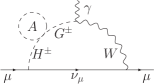
(a)

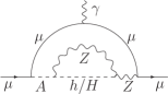
(b)

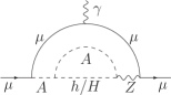
(c)

Figure 12: The Feynman diagrams containing $A$ with Yukawa couplings.

Fig. 12 shows the only remaining two-loop Feynman diagram with $M_{A}$ and Yukawa coupling dependence. The sum of the diagrams of Figs. 12(b) and 12(c) is zero, therefore these give no contributions. The remaining possible $M_{A}$ dependence can arise from the diagram of Fig. 12(a). However, as we show in the following this contribution cancels out with the tadpole counterterm contribution.

The sum of the two-loop Feynman diagram Fig. 12(a) and the counterterm diagram Fig. 1(c) with tadpole counterterm containing only $A$-loop can be illustrated as

(134)

The explicit form of the $H^{\pm}$-$G^{\pm}$ mixing propagator counterterm is

(135)

where

$$\delta t_{HG}\,= \,\cos(\beta-\alpha)\delta T_{h}-\sin(\beta-\alpha)\delta T_{H} \simeq\,-\delta T_{H}+\eta\,\delta T_{h}+{\cal O}(\eta^{2}).$$ (136)

According to the definition of the tadpole counterterms, the $A$ Higgs boson contribution to the tadpole counterterm for $h$ is the product of the $(h-A-A)$ coupling constant and the scalar one-point loop function $A_{0}(m)$,

(137)

For $H$ we need to replace the $(h-A-A)$ with $(H-A-A)$ coupling constant, and the result reads

(138)

By combining the previous equations we obtain for Eq. (135)

$$\frac{i\,g_{2}}{2\,M_{W}}\,\delta t_{HG}\,= \,\frac{-i\,g_{2}^{2}}{4\,M_{W}^{2}}\,A_{0}(M_{A})\,\times$$

$$\left\{(M_{H}^{2}-\frac{\Lambda_{5}\,v^{2}}{2})\left(t_{\beta}-\frac{1}{t_{\beta}}\right)+(M_{H}^{2}-M_{h}^{2})\eta\right\}.$$ (139)

This shows that the $M_{A}$ dependence is now only localized in $A_{0}(M_{A})$. On the other hand, after applying the quartic coupling constant of $H^{\pm}$-$G^{\pm}$-$A$-$A$, we obtain the explicit form of the inner loop of Fig. 12, with the result

(140)

Hence, the $M_{A}$ dependent parts vanish,

(141)

Here we provide corrections to our paper. The corrections are mostly typos in the formulas printed in the paper which do not affect the analytic results implemented in our codes for the numerical analyses. In addition to the typo corrections we improve our approximation formula, eq. (67) and the corresponding plots in figures 10 and 11 as explained below. In this context we also mention that the phenomenological discussions of the present paper are updated and superseded by the ones of our successive paper [1].

1. In the Lagrangian eq. (16), the abbreviation $y_{f}^{H^{\pm}}$ for the Yukawa coupling of the charged Higgs was not defined. Here we provide a slightly rewritten version of the Lagrangian, including all necessary definitions. It assumes $CP$ conservation and all appearing abbreviations to be real and reads

   $${\cal{L}}_{Y}= \sqrt{2}H^{+}\big{(}{\mathrm{bar}{u}}[V_{\text{CKM}}\,y_{d}^{H^{\pm}}P_{\text{R}}+y_{u}^{H^{\pm}}V_{\text{CKM}}P_{\text{L}}]d+{\mathrm{bar}{\nu}}y_{l}^{H^{\pm}}P_{\text{R}}l\big{)}$$

   $$-\sum_{f}\,h{\mathrm{bar}{f}}y_{f}^{h}P_{\text{R}}f-\sum_{f}\,H{\mathrm{bar}{f}}y_{f}^{H}P_{\text{R}}f+i\sum_{f}\,A{\mathrm{bar}{f}}y_{f}^{A}P_{\text{R}}f+h.c..$$

   The Yukawa couplings in eq. (18) should be replaced by

   $$Y^{h}_{f}= \sin(\beta-\alpha)+\cos(\beta-\alpha)\zeta_{f},$$

   $$Y^{H}_{f}= \cos(\beta-\alpha)-\sin(\beta-\alpha)\zeta_{f},$$

   $$Y^{H^{\pm}}_{d,l}=Y^{A}_{d,l}= -\zeta_{d,l},\quad Y^{H^{\pm}}_{u}=Y^{A}_{u}=\zeta_{u},$$

   and those in eq. (19) should be replaced by

   $$Y^{h}_{f}= 1+\eta\zeta_{f},\quad Y^{H}_{f}=-\zeta_{f}+\eta,\quad Y^{H^{\pm}}_{f}=Y^{A}_{f}=-\Theta^{A}_{f}\zeta_{f},$$

   $$\Theta^{A}_{d,l}= 1,\qquad\Theta^{A}_{u}=-1,\qquad\Theta^{H}_{u,d,l}=1,$$

   which includes $Y_{f}^{H^{\pm}}$.

2. In eq. (51) $v$ is missing in the triple Higgs coupling constant. The correct formula is

   $$g_{H,H^{\pm},H^{\mp}}\propto\left\{\left(t_{\beta}-\frac{1}{t_{\beta}}\right)\frac{v}{2}\left(\Lambda_{5}-2\,\frac{M_{H}^{2}}{v^{2}}\right)\right.\\ \left.\,\,+\eta\,v\left(\Lambda_{5}-\frac{M_{H}^{2}}{v^{2}}-2\frac{M_{H^{\pm}}^{2}}{v^{2}}\right)\right\}.$$

3. Page 25, line 2: $M_{l}=\{(m_{e},0),(m_{\mu},0),(m_{\tau},0)\}$.

4. There was an unnecessary, extra ${\Phi}(x_{d}^{1/2},x_{u}^{1/2},1)$ in the second line of eq. (61), and its corrected version reads

   $$\mathcal{F}^{H^{\pm}}_{d}(M_{d})=-(x_{u}-x_{d})+\left[\frac{\mathrm{bar}{c}}{y}-c\left(\frac{x_{u}-x_{d}}{y}\right)\right]{\Phi}(x_{d}^{1/2},x_{u}^{1/2},1)$$

   $$\quad\quad\quad\quad\quad\quad+c\left[\mbox{Li}_{2}\left(1-\frac{x_{d}}{x_{u}}\right)-\frac{1}{2}\ln(x_{u})\ln\left(\frac{x_{d}}{x_{u}}\right)\right]$$

   $$\quad\quad\quad\quad\quad\quad+\left(s+x_{d}\right)\ln(x_{d})+\left(s-x_{u}\right)\ln(x_{u}).$$

5. A factor of $-\frac{1}{2}$ was missing in eq. (78), and the correct expression is

   $${\mathcal{T}}_{7}(u,\omega)= -\frac{f_{5}}{2}(2(u+\omega)-(u-\omega)^{2}-1)\ln\left(\frac{{\mathcal{S}}_{1}(u,\omega)}{2\sqrt{u\omega}}\right)$$

   $$\times\left(u+\omega-1-\frac{4u\omega}{{\mathcal{S}}_{1}(u,\omega)}\right).$$

6. In the numerical evaluation of our results we have used one-loop corrected relationships between the electroweak parameters: $s_{W}$, $c_{W}$, $M_{W}$, $M_{Z}$, $v$. In this way, the numerical evaluation of $a_{\mu}$ contains certain terms which are formally of 3-loop order but which do not correspond to a full 3-loop calculation. In the following we provide results based on an evaluation which uses tree-level relationships between these electroweak parameters and which thereby corresponds to a pure 2-loop calculation in the on-shell renormalization scheme.

   According to the original numerical implementation, there was a slight increase with $t_{\beta}$ visible in the original figure 10a, and figures 10d and 11 for $t_{\beta}=100$ were affected by the incomplete 3-loop effects mentioned above. Actually, the linear large-$t_{\beta}$-enhancement vanishes in the new, strict 2-loop evaluation. This can be understood with the help of eq. (67). This equation can now be analytically evaluated by using the tree-level relationships for the electroweak parameters in eqs. (15) and (99). In this case, the term proportional to $M_{H}^{2}\zeta_{l}t_{\beta}$ on the far right-hand side of eq. (67) analytically vanishes. In the approximation of large $t_{\beta}$, the far right-hand side of eq. (67) contains only terms which decrease or approach a constant for large $t_{\beta}$.

   Here we provide revised versions of the plots in figures 10 and 11 with the modified numerical evaluation using tree-level relations between electroweak parameters: see figures 13 and 14. Here the linear increase in $t_{\beta}$ is absent and the numerical results in the large $t_{\beta}$ regime are slightly changed. Again, we refer to Ref. [1] for a more detailed phenomenological evaluation which also takes into account a variety of experimental constraints on the input parameters $\zeta_{l}$, $t_{\beta}$, and $\eta$.

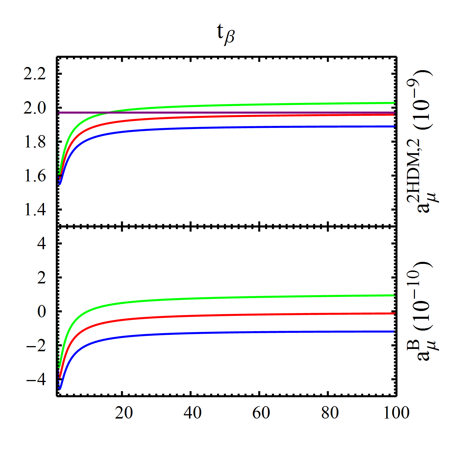
(a)

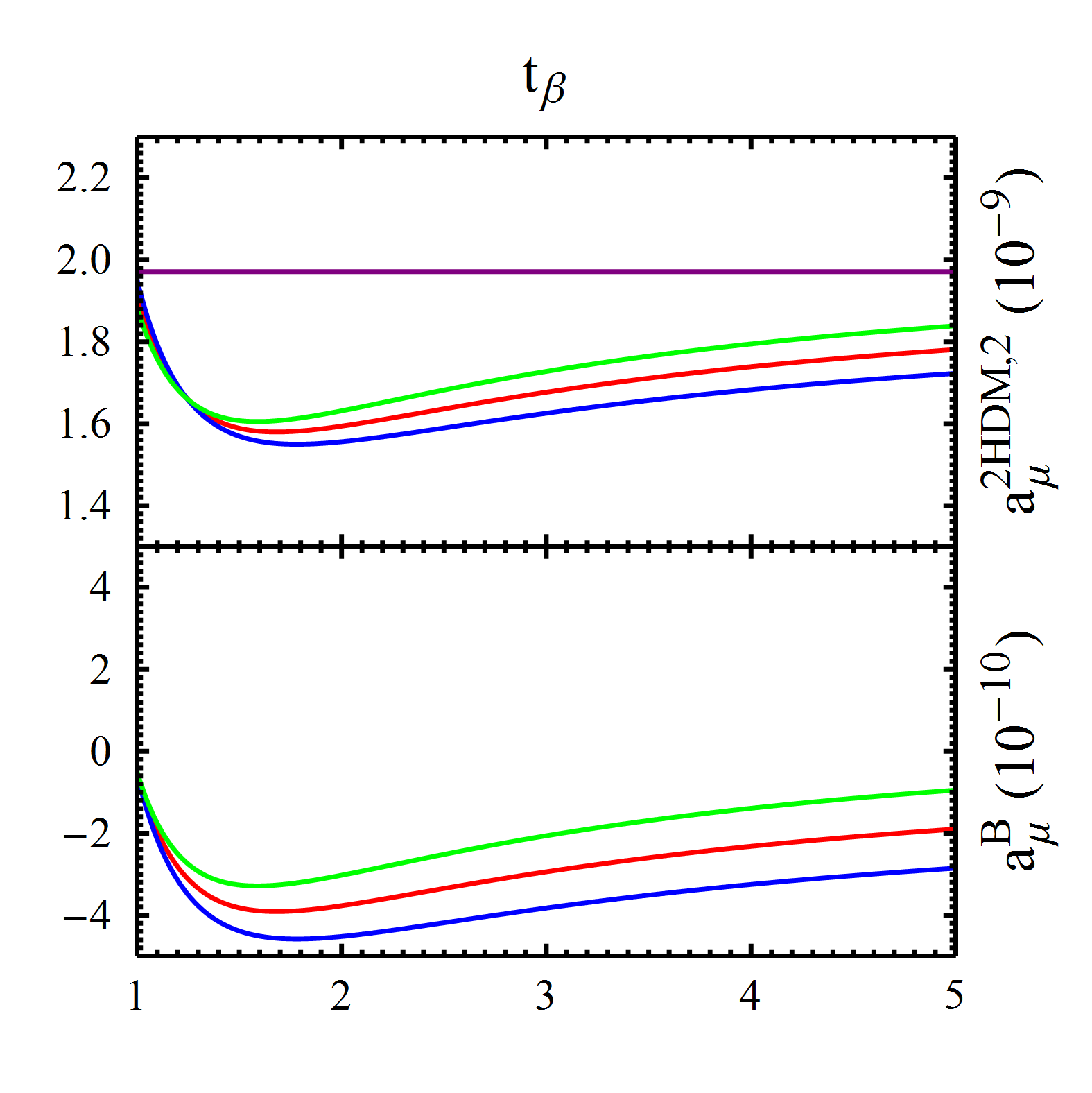
(b)

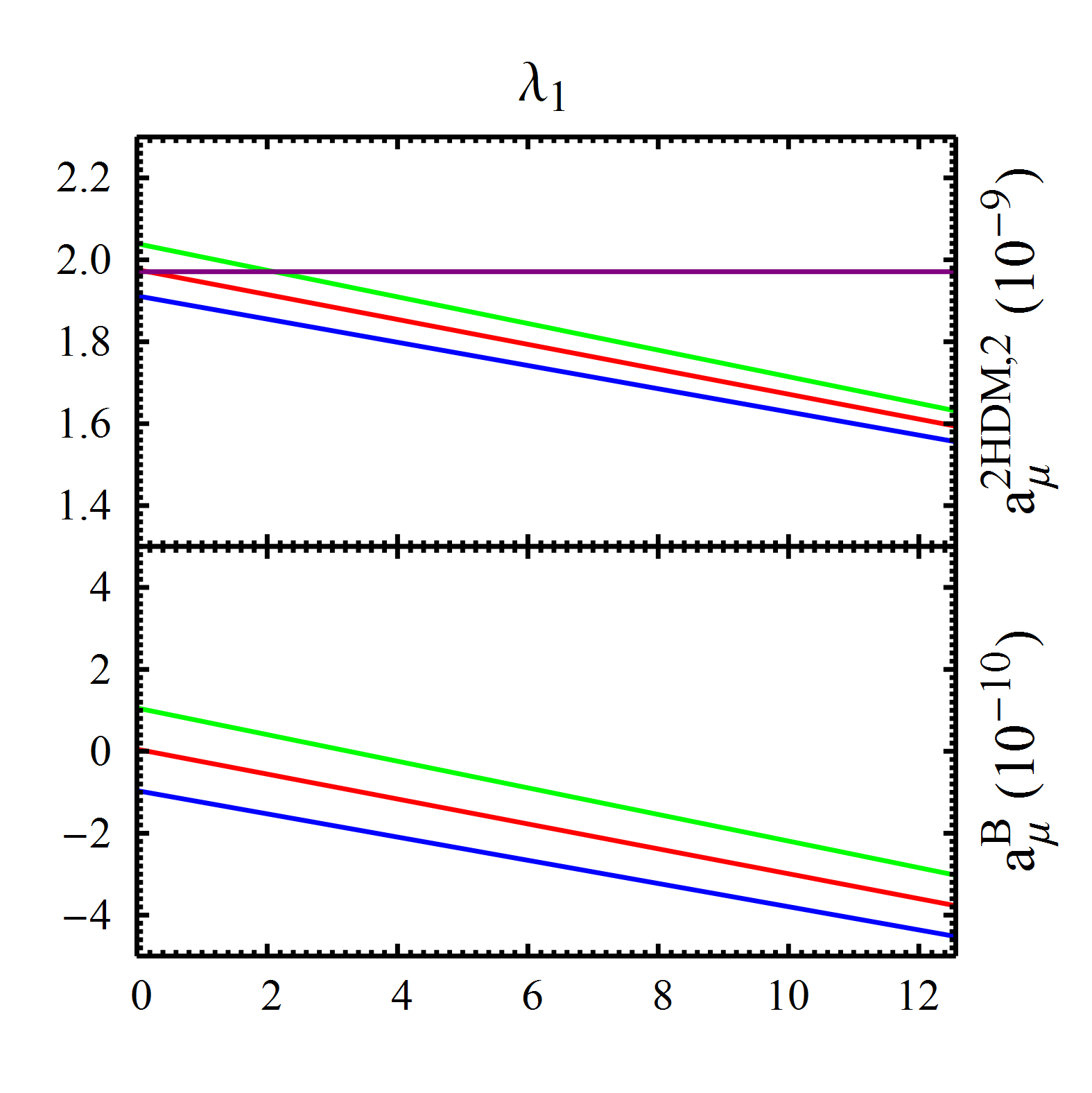
(c)

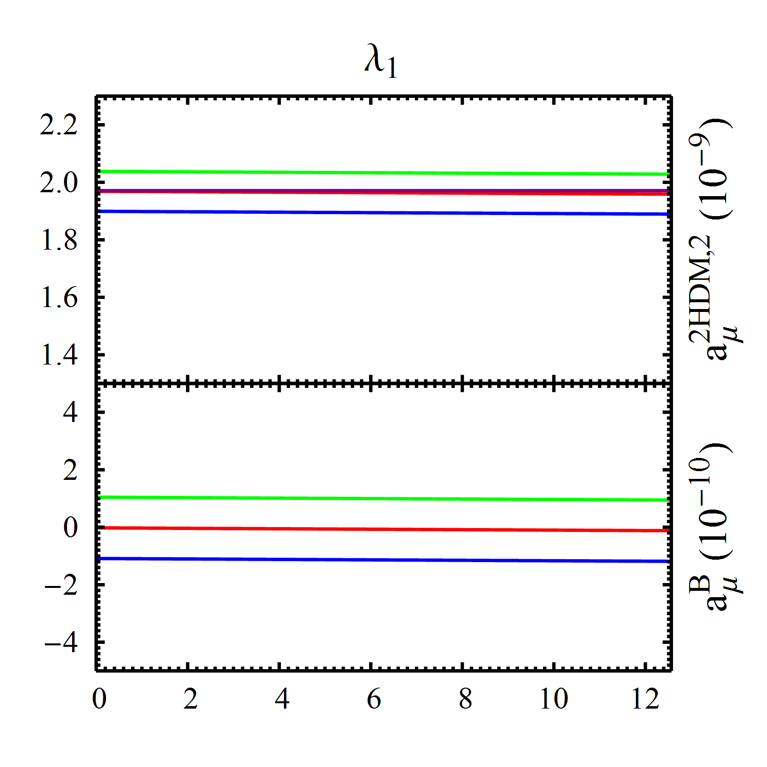
(d)

Figure 13: Revised version of figure 10. Plots showing the behavior of $a_{\mu}^{{\text{2HDM}},2}$, and $a_{\mu}^{\text{B}}$. Each red/blue/green line is for $\eta=0/0.1/-0.1$. $t_{\beta}$ varies for (a) and (b), and $\lambda_{1}$ for (c) and (d). We consider the representative mass parameter point in eq. (4.3). $\lambda_{1}=4\pi$ for (a) and (b). We employ $t_{\beta}=2$ and $t_{\beta}=100$ for (c) and (d) respectively.

References

- [1] G. Aad et al. [ATLAS Collaboration], Phys. Lett. B 716 (2012) 1 [arXiv:1207.7214 [hep-ex]].
- [2] S. Chatrchyan et al. [CMS Collaboration], Phys. Lett. B 716 (2012) 30 [arXiv:1207.7235 [hep-ex]].
- [3] M. Dührssen, talk given at 50th Rencontres de Moriond EW 2015;
- [4] A. Czarnecki and W. J. Marciano, Phys. Rev. D 64 (2001) 013014 [hep-ph/0102122].
- [5] D. W. Hertzog, J. P. Miller, E. de Rafael, B. Lee Roberts and D. Stöckinger, arXiv:0705.4617.
- [6] D. Stöckinger, in Lepton Dipole Moments, B. L. Roberts and W. J. Marciano Eds., Adv. Ser. Direct. High Energy Phys. 20 (2009) 393,
- [7] G.W. Bennett, et al., (Muon Collaboration), Phys. Rev. D 73, 072003 (2006).
- [8] M. Davier, A. Hoecker, B. Malaescu and Z. Zhang, Eur. Phys. J. C 71 (2011) 1515 [Erratum-ibid. C 72 (2012) 1874] [arXiv:1010.4180 [hep-ph]].
- [9] K. Hagiwara, R. Liao, A. D. Martin, D. Nomura and T. Teubner, J. Phys. G 38 (2011) 085003 [arXiv:1105.3149 [hep-ph]].
- [10] T. Aoyama, M. Hayakawa, T. Kinoshita and M. Nio, Phys. Rev. Lett. 109, 111808 (2012) [arXiv:1205.5370 [hep-ph]].
- [11] C. Gnendiger, D. Stöckinger and H. Stöckinger-Kim, Phys. Rev. D 88, 053005 (2013) [arXiv:1306.5546 [hep-ph]].
- [12] A. L. Kataev, Phys. Rev. D 86 (2012) 013010 [arXiv:1205.6191 [hep-ph]].
- [13] R. Lee, P. Marquard, A. V. Smirnov, V. A. Smirnov and M. Steinhauser, JHEP 1303 (2013) 162 [arXiv:1301.6481 [hep-ph]]; A. Kurz, T. Liu, P. Marquard and M. Steinhauser, Nucl. Phys. B 879 (2014) 1 [arXiv:1311.2471 [hep-ph]]; A. Kurz, T. Liu, P. Marquard, A. V. Smirnov, V. A. Smirnov and M. Steinhauser, Phys. Rev. D 92 (2015) no.7, 073019 [arXiv:1508.00901 [hep-ph]]; Phys. Rev. D 93 (2016) no.5, 053017 [arXiv:1602.02785 [hep-ph]].
- [14] F. Jegerlehner and R. Szafron, Eur. Phys. J. C 71 (2011) 1632 [arXiv:1101.2872 [hep-ph]].
- [15] M. Benayoun, P. David, L. DelBuono and F. Jegerlehner, Eur. Phys. J. C 73 (2013) 2453 [arXiv:1210.7184 [hep-ph]]; Eur. Phys. J. C 75 (2015) no.12, 613 [arXiv:1507.02943 [hep-ph]]; arXiv:1605.04474 [hep-ph].
- [16] A. Kurz, T. Liu, P. Marquard and M. Steinhauser, Phys. Lett. B 734 (2014) 144 [arXiv:1403.6400 [hep-ph]].
- [17] G. Colangelo, M. Hoferichter, A. Nyffeler, M. Passera and P. Stoffer, Phys. Lett. B 735 (2014) 90 [arXiv:1403.7512 [hep-ph]].
- [18] G. Colangelo, M. Hoferichter, M. Procura and P. Stoffer, JHEP 1409 (2014) 091 [arXiv:1402.7081 [hep-ph]]; G. Colangelo, M. Hoferichter, B. Kubis, M. Procura and P. Stoffer, Phys. Lett. B 738 (2014) 6 [arXiv:1408.2517 [hep-ph]]; G. Colangelo, M. Hoferichter, M. Procura and P. Stoffer, JHEP 1509 (2015) 074 [arXiv:1506.01386 [hep-ph]].
- [19] V. Pauk and M. Vanderhaeghen, Phys. Rev. D 90 (2014) 11, 113012 [arXiv:1409.0819 [hep-ph]].
- [20] T. Blum, S. Chowdhury, M. Hayakawa and T. Izubuchi, Phys. Rev. Lett. 114 (2015) 1, 012001 [arXiv:1407.2923 [hep-lat]]; T. Blum, N. Christ, M. Hayakawa, T. Izubuchi, L. Jin and C. Lehner, Phys. Rev. D 93 (2016) no.1, 014503 [arXiv:1510.07100 [hep-lat]].
- [21] M. Ablikim et al. [BESIII Collaboration], Phys. Lett. B 753, 629 (2016) [arXiv:1507.08188 [hep-ex]].
- [22] B. Chakraborty, C. T. H. Davies, J. Koponen, G. P. Lepage, M. J. Peardon and S. M. Ryan, Phys. Rev. D 93 (2016) no.7, 074509 [arXiv:1512.03270 [hep-lat]].
- [23] F. Jegerlehner and A. Nyffeler, Phys. Rept. 477, 1 (2009) [arXiv:0902.3360 [hep-ph]].
- [24] J. P. Miller, E. de Rafael, B. L. Roberts and D. Stöckinger, Ann. Rev. Nucl. Part. Sci. 62, 237 (2012).
- [25] T. Blum, A. Denig, I. Logashenko, E. de Rafael, B. L. Roberts, T. Teubner and G. Venanzoni, arXiv:1311.2198 [hep-ph].
- [26] M. Benayoun, J. Bijnens, T. Blum, I. Caprini, G. Colangelo, H. Czyz, A. Denig and C. A. Dominguez et al., arXiv:1407.4021 [hep-ph].
- [27] K. Melnikov, EPJ Web Conf. 118 (2016) 01020.
- [28] A. Broggio, E. J. Chun, M. Passera, K. M. Patel and S. K. Vempati, JHEP 1411 (2014) 058 [arXiv:1409.3199 [hep-ph]].
- [29] L. Wang and X. F. Han, JHEP 1505, 039 (2015) [arXiv:1412.4874 [hep-ph]].
- [30] V. Ilisie, JHEP 1504 (2015) 077 [arXiv:1502.04199 [hep-ph]].
- [31] T. Abe, R. Sato and K. Yagyu, JHEP 1507, 064 (2015) [arXiv:1504.07059 [hep-ph]].
- [32] A. Crivellin, J. Heeck and P. Stoffer, Phys. Rev. Lett. 116 (2016) no.8, 081801 [arXiv:1507.07567 [hep-ph]].
- [33] E. J. Chun, Z. Kang, M. Takeuchi and Y. L. S. Tsai, JHEP 1511 (2015) 099 [arXiv:1507.08067 [hep-ph]].
- [34] T. Han, S. K. Kang and J. Sayre, JHEP 1602, 097 (2016) [arXiv:1511.05162 [hep-ph]].
- [35] S. M. Barr and A. Zee, Phys. Rev. Lett. 65 (1990) 21 [Erratum-ibid. 65 (1990) 2920].
- [36] D. Chang, W. F. Chang, C. H. Chou and W. Y. Keung, Phys. Rev. D 63 (2001) 091301 doi:10.1103/PhysRevD.63.091301 [hep-ph/0009292].
- [37] K. m. Cheung, C. H. Chou and O. C. W. Kong, Phys. Rev. D 64 (2001) 111301 doi:10.1103/PhysRevD.64.111301 [hep-ph/0103183].
- [38] Y. L. Wu and Y. F. Zhou, Phys. Rev. D 64 (2001) 115018 doi:10.1103/PhysRevD.64.115018 [hep-ph/0104056].
- [39] M. Krawczyk, Acta Phys. Polon. B 33 (2002) 2621 [hep-ph/0208076].
- [40] R. M. Carey, K. R. Lynch, J. P. Miller, B. L. Roberts, W. M. Morse, Y. K. Semertzides, V. P. Druzhinin and B. I. Khazin et al., FERMILAB-PROPOSAL-0989. B. L. Roberts, Chin. Phys. C 34 (2010) 741 [arXiv:1001.2898 [hep-ex]].
- [41] H. Iinuma [J-PARC New g-2/EDM experiment Collaboration], J. Phys. Conf. Ser. 295 (2011) 012032.
- [42] A. Czarnecki, B. Krause and W. J. Marciano, Phys. Rev. Lett. 76 (1996) 3267 [hep-ph/9512369]. A. Czarnecki, B. Krause and W. J. Marciano, Phys. Rev. D 52 (1995) 2619 [hep-ph/9506256].
- [43] A. Czarnecki, W. J. Marciano and A. Vainshtein, Phys. Rev. D 67 (2003) 073006 Erratum: [Phys. Rev. D 73 (2006) 119901] [hep-ph/0212229].
- [44] S. Heinemeyer, D. Stöckinger and G. Weiglein, Nucl. Phys. B 699 (2004) 103.
- [45] S. Heinemeyer, D. Stöckinger and G. Weiglein, Nucl. Phys. B 690 (2004) 62.
- [46] A. Arhrib and S. Baek, Phys. Rev. D 65 (2002) 075002 [hep-ph/0104225].
- [47] C. H. Chen and C. Q. Geng, Phys. Lett. B 511 (2001) 77 [arXiv:hep-ph/0104151].
- [48] K. Cheung, O. C. W. Kong and J. S. Lee, JHEP 0906 (2009) 020 [arXiv:0904.4352 [hep-ph]].
- [49] P. von Weitershausen, M. Schäfer, H. Stöckinger-Kim and D. Stöckinger, Phys. Rev. D 81 (2010) 093004 [arXiv:1003.5820 [hep-ph]].
- [50] H. G. Fargnoli, C. Gnendiger, S. Paßehr, D. Stöckinger and H. Stöckinger-Kim, Phys. Lett. B 726 (2013) 717 [arXiv:1309.0980 [hep-ph]].
- [51] H. G. Fargnoli, C. Gnendiger, S. Paßehr, D. Stöckinger and H. Stöckinger-Kim, JHEP 1402 (2014) 070 [arXiv:1311.1775 [hep-ph]].
- [52] D. Stöckinger, J. Phys. G 34 (2007) R45.
- [53] P. Athron et al., Eur. Phys. J. C 76 (2016) no.2, 62 [arXiv:1510.08071 [hep-ph]].
- [54] G. C. Branco, P. M. Ferreira, L. Lavoura, M. N. Rebelo, M. Sher and J. P. Silva, Phys. Rept. 516, 1 (2012) [arXiv:1106.0034 [hep-ph]].
- [55] J. F. Gunion and H. E. Haber, Phys. Rev. D 67, 075019 (2003) [hep-ph/0207010].
- [56] A. Celis, V. Ilisie and A. Pich, JHEP 1312, 095 (2013) [arXiv:1310.7941 [hep-ph]].
- [57] T. Hahn, Comput. Phys. Commun. 140 (2001) 418–431 [arXiv:0012260 [hep-ph]].
- [58] A. Pich and P. Tuzon, Phys. Rev. D 80, 091702 (2009) [arXiv:0908.1554 [hep-ph]].
- [59] M. Krause, R. Lorenz, M. Muhlleitner, R. Santos and H. Ziesche, JHEP 1609 (2016) 143 doi:10.1007/JHEP09(2016)143 [arXiv:1605.04853 [hep-ph]].
- [60] A. Denner, L. Jenniches, J. N. Lang and C. Sturm, JHEP 1609 (2016) 115 doi:10.1007/JHEP09(2016)115 [arXiv:1607.07352 [hep-ph]].
- [61] P. M. Ferreira and D. R. T. Jones, JHEP 0908, 069 (2009) [arXiv:0903.2856 [hep-ph]].
- [62] A. Barroso, P. M. Ferreira, I. P. Ivanov and R. Santos, JHEP 1306, 045 (2013) [arXiv:1303.5098 [hep-ph]].
- [63] M. E. Peskin and T. Takeuchi, Phys. Rev. Lett. 65, 964 (1990).
- [64] K. A. Olive et al. [Particle Data Group Collaboration], Chin. Phys. C 38, 090001 (2014).
- [65] D. Eriksson, J. Rathsman and O. Stal, Comput. Phys. Commun. 181, 189 (2010) [arXiv:0902.0851 [hep-ph]].
- [66] D. Eriksson, J. Rathsman and O. Stal, Comput. Phys. Commun. 181, 833 (2010).
- [67] G. Weiglein, R. Scharf and M. Böhm, Nucl. Phys. B 416 (1994) 606 [hep-ph/9310358].
- [68] B. e. Lautrup, A. Peterman and E. de Rafael, Phys. Rept. 3 (1972) 193.
- [69] J. P. Leveille, Nucl. Phys. B 137 (1978) 63.
- [70] A. Dedes and H. E. Haber, JHEP 0105 (2001) 006 [hep-ph/0102297].
- [71] S. Bertolini, Nucl. Phys. B 272, 77 (1986).
- [72] D. Lopez-Val and J. Sola, Eur. Phys. J. C 73, 2393 (2013) [arXiv:1211.0311 [hep-ph]].
- [73] A. Denner, Fortsch. Phys. 41, 307 (1993) [arXiv:0709.1075 [hep-ph]].
- [74] R. Santos and A. Barroso, Phys. Rev. D 56, 5366 (1997) [hep-ph/9701257].
- [75] M. A. Caprio, Comput. Phys. Commun. 171, 107 (2005)
- [76] A. I. Davydychev and J. B. Tausk, Nucl. Phys. B 397, 123 (1993).
Erratum: The muon magnetic moment in the 2HDM: complete two-loop result
Adriano Cherchiglia, Patrick Kneschke, Dominik Stöckinger,
Hyejung Stöckinger-Kim
Institut für Kern- und Teilchenphysik, TU Dresden, 01069 Dresden, Germany

References

- [1] A. Cherchiglia, D. Stöckinger and H. Stöckinger-Kim, Muon g-2 in the 2HDM: maximum results and detailed phenomenology, Phys. Rev. D 98 (2018), 035001 [arXiv:1711.11567 [hep-ph]].