Topological Data Analysis with Bregman Divergences

Abstract.

Given a finite set in a metric space, the topological analysis generalizes hierarchical clustering using a 1-parameter family of homology groups to quantify connectivity in all dimensions. The connectivity is compactly described by the persistence diagram. One limitation of the current framework is the reliance on metric distances, whereas in many practical applications objects are compared by non-metric dissimilarity measures. Examples are the Kullback–Leibler divergence, which is commonly used for comparing text and images, and the Itakura–Saito divergence, popular for speech and sound. These are two members of the broad family of dissimilarities called Bregman divergences.

We show that the framework of topological data analysis can be extended to general Bregman divergences, widening the scope of possible applications. In particular, we prove that appropriately generalized Čech and Delaunay (alpha) complexes capture the correct homotopy type, namely that of the corresponding union of Bregman balls. Consequently, their filtrations give the correct persistence diagram, namely the one generated by the uniformly growing Bregman balls. Moreover, we show that unlike the metric setting, the filtration of Vietoris-Rips complexes may fail to approximate the persistence diagram. We propose algorithms to compute the thus generalized Čech, Vietoris-Rips and Delaunay complexes and experimentally test their efficiency. Lastly, we explain their surprisingly good performance by making a connection with discrete Morse theory.

1. Introduction

The starting point for the work reported in this paper is the desire to extend the basic topological data analysis (TDA) paradigm to data measured with dissimilarities. In particular for high-dimensional data, such as discrete probability distributions, notions of dissimilarity inspired by information theory behave strikingly different from the Euclidean distance, which is the usual setting for TDA. On the practical side, the Euclidean distance is particularly ill-suited for many types of high-dimensional data; see for example [22], which provides evidence that the Euclidean distance consistently performs the worst among several dissimilarity measures across a range of text-retrieval tasks. A broad class of dissimilarities are the Bregman divergences [9]. Its most prominent members are the Kullback–Leibler divergence [24], which is commonly used both for text documents [6, 22] and for images [15], and the Itakura–Saito divergence [23], which is popular for speech and sound data [19]. We propose a TDA framework in the setting of Bregman divergences. Since TDA and more generally computational topology are young and emerging fields, we provide some context for the reader. For more a comprehensive introduction, see the recent textbook [17].

Computational topology.

Computational topology is an algorithmic approach to describing shape in a coarser sense than computational geometry does. TDA utilizes such algorithms within data analysis. One usually works with a finite set of points, possibly embedded in a high-dimensional space. Such data may be viewed as a collection of balls of a radius that depends on the scale of interest. Intersections reveal the connectivity of the data. For example, the components of the intersection graph correspond to the components of the union of balls.

Homology groups.

These are studied in the area of algebraic topology, where they are used to describe and analyze topological spaces; see e.g. [21]. The connected components of a space or, dually, the gaps between them are encoded in its zero-dimensional homology group. There is a group for each dimension. For example, the one-dimensional group encodes loops or, dually, the tunnels, and the two-dimensional group encodes closed shells or, dually, the voids. Importantly, homology provides a formalism to talk about different kinds of connectivity and holes of a space that allows for fast algorithms.

Nerves and simplicial complexes.

The nerve of a collection of balls generalizes the intersection graph and contains a $k$-dimensional simplex for every $k+1$ balls that have a non-empty common intersection. It is a hypergraph that is closed under taking subsets, a structure known as a simplicial complex in topology. If the balls are convex, then the Nerve Theorem states that this combinatorial construction captures the topology of the union of balls. More precisely, the nerve and the union have the same homotopy type and therefore isomorphic homology groups [8, 25]. This result generalizes to the case in which the balls are not necessarily convex but their common intersections of all orders are contractible. In the context in which we center a ball of some radius at each point of a given set, the nerve is referred to as the Čech complex of the points for the given radius. Its $k$-skeleton is obtained by discarding simplices of dimension greater than $k$. The practice-oriented reader will spot a flaw in this setup: fixing the radius is a serious drawback that limits data analysis applications.

Persistent homology.

To remedy this deficiency, we study the evolution of the topology across all scales, thus developing what we refer to as persistent homology. For graphs and connected components, this idea is natural but more difficult to flesh out in full generality. In essence, one varies the radius of balls from $0$ to $\infty$, giving rise to a nested sequence of spaces, called a filtration. Topological features, namely homology classes of different dimensions, are created and destroyed along the way. In practice, one computes the persistence diagram of a filtration, which discriminates topological features based on their lifetime, or persistence. The persistence diagram serves as a compact topological descriptor of a dataset, which is provably robust against noise. Owing to its algebraic and topological foundations, the theory is very general. Importantly, the Nerve Theorem extends to filtrations [12, Lemma 3.4], so we can often restrict our considerations to complexes for a fixed radius. Moreover, the existing algorithms for persistence diagrams can be used without modification.

TDA in the Bregman setting.

In the light of the above, there are only two obstacles to applying topological data analysis to data measured with Bregman divergences. We need to prove that the Nerve Theorem applies also when the balls are induced by Bregman divergences, and we need to provide efficient algorithms to construct the relevant complexes. The main complication is that the balls may be nonconvex, which we overcome by combining results from convex analysis and topology.

Applications.

Persistence is an important method within TDA, which has been successfully used in a variety of applications. In low dimensions, it was for example used to shed light on the distribution of matter in the Universe [32] and to characterize the structure of atomic configurations in silica glass [26]. As for high-dimensional data, Chan et al. analyze viral DNA and relate persistent cycles with recombinations [11], and Port et al. study languages leaving the interpretation of a persistent cycle in the Indo-Germanic family open [29].

Related work.

This paper is the first work at the intersection of topology and Bregman divergences. We list related papers in relevant fields. In machine learning, Banerjee et al. use the family of Bregman divergences as the unifying framework for clustering algorithms [3]. The field of information geometry deals with selected Bregman divergences and related concepts from a geometric perspective [2]. Building on the classical work of Rockafellar [31] in convex analysis, Bauschke and Borwein are the first to use the Legendre transform for analyzing Bregman divergences [5]. Boissonnat, Nielsen and Nock [7] use similar methods to make significant contributions at the intersection of computational geometry and Bregman divergences. In particular, they study the geometry of Bregman balls and Delaunay triangulations, but not the topologically more interesting Delaunay, or alpha, complexes. In the Euclidean setting, the basic constructions are well understood [4, 34], including approximations, which are interesting and useful, but beyond the scope of this paper.

Results.

This paper provides the first general TDA framework that applies to high-dimensional data measured with non-metric dissimilarities. Indeed, prior high-dimensional applications of TDA were restricted to low-dimensional homology, required custom-made topological results, or used common metrics such as the Euclidean and the Hamming distances, which are often not good choices for such data. We list the main technical contributions:

1. We show that the balls under any Bregman divergence have common intersections that are either empty of contractible.

2. We show that the persistence diagram of the Vietoris–Rips complex can be arbitrarily far from that of the filtration of the union on Bregman balls.

3. We show that the radius functions that correspond to the Čech and Delaunay complexes for Bregman divergences are generalized discrete Morse functions.

4. We develop algorithms for computing Čech and Delaunay radius functions for Bregman divergences, which owe their speed to non-trivial structural properties implied by Result 3.

Most fundamental of the four is Result 1, which forms the theoretical foundation of TDA in the Bregman setting. It implies that the Čech and Delaunay complexes for a given radius have the same homotopy type as the union of Bregman balls. Combined with the Nerve Theorem for filtrations, it also implies that the filtration of Čech and Delaunay complexes have the same persistence diagram as the filtration of the unions. In the practice of TDA, the filtration of Vietoris–Rips complexes is often substituted for the filtration of Čech or Delaunay complexes. For metrics, this is justified by the small bottleneck distance between the persistence diagrams if drawn in log-log scale. Result 2 shows that such a substitution is not generally justified for Bregman divergences. In other words, for some Bregman divergences higher order interactions have to be taken into account explicitly as they are not approximated by implications of pairwise interactions. To appreciate Results 3 and 4, we note that the Čech radius function maps every simplex to the smallest radius, $r$, such that the simplex belongs to the Čech complex for radius $r$, and similarly for Delaunay. Being a generalized discrete Morse function has important structural consequences that make it possible to construct Čech and Delaunay complexes in an output-sensitive manner. We support this claim with experiments.

Implications.

Our results open up a new area of research at the intersection of geometry, topology, algorithms and data analysis. On the application side, it enables TDA for a wide variety of data. Moreover, it connects topology with information theory and statistics, where Bregman divergences play a significant role. Finally, efficient algorithms and data structures are needed to handle large datasets. Considerable progress has been made within the TDA community, but we believe a collaboration with the wider computer science community would be fruitful.

Scope.

The aim of this paper is to show that the machinery of persistent homology is applicable to different kinds of high-dimensional data. While questions remain, we provide a solid foundation for further developments.

Outline.

Section 2 reviews the concept of Bregman divergences, including an elementary description of the Legendre transform. Section 3 proves the contractibility of common intersections of Bregman balls and introduces Čech, Delaunay, and Vietoris–Rips complexes in the Bregman setting. Section 4 introduces the Čech and Delaunay radius functions and explains algorithms for constructing them. Section 5 concludes this paper.

2. Bregman Divergences

Bregman divergences are sometimes called distances because they measure dissimilarity. As we will see shortly, they are generally not symmetric, and they always violate the triangle inequality. So really they satisfy only the first axiom of a metric, mapping ordered pairs to non-negative numbers and to zero iff the two elements are equal.

We begin with a formal introduction of the concept, which originated in the paper by Bregman [9]. Their basic properties are well known; see the recent paper by Boissonnat, Nielsen and Nock [7]. We stress that our setting is slightly different: following Bauschke and Borwein [5], we define the divergences in terms of functions of Legendre type. The crucial benefit of this additional requirement is that the conjugate of a function of Legendre type is again a function of Legendre type, even if the domain is bounded as in the important case of the standard simplex. In contract, the conjugate of a differentiable and strictly convex function that is not of Legendre type is not necessarily again a convex function.

Functions of Legendre type.

Let ${\Omega}\subseteq{\mathbb{R}}^{n}$ be an nonempty open convex set and ${{F}}\colon{\Omega}\to{\mathbb{R}}$ a strictly convex differentiable function. In addition, we require that the length of the gradient of ${{F}}$ goes to infinity whenever we approach the boundary of ${\Omega}$. Following [31, page 259], we say that ${{F}}\colon{\Omega}\to{\mathbb{R}}$ is a function of Legendre type. As suggested by the naming convention, these conditions are crucial when we apply the Legendre transform to ${{F}}$. The last condition prevents us from arbitrarily restricting the domain and is vacuous whenever ${\Omega}$ does not have a boundary, for example when ${\Omega}={\mathbb{R}}^{n}$. For points $x,y\in{\Omega}$, the Bregman divergence from $x$ to $y$ associated with ${{F}}$ is the difference between ${{F}}$ and the best linear approximation of ${{F}}$ at $y$, both evaluated at $x$:

$${D}_{{{F}}}{({x}\|{y})} ={{F}}(x)-\left[{{F}}(y)+{\langle\nabla{{F}}(y),x-y\rangle}\right].$$ (1)

As illustrated in Figure 1, we get ${{D}_{{{F}}}{({x}\|{y})}}$ by first drawing the hyperplane that touches the graph of ${{F}}$ at the point $(y,{{F}}(y))$. We then intersect the vertical line that passes through $x$ with the graph of ${{F}}$ and the said hyperplane: the Bregman divergence is the height difference between the two intersections. Note that it is not necessarily symmetric: ${{D}_{{{F}}}{({x}\|{y})}}\neq{{D}_{{{F}}}{({y}\|{x})}}$ for most ${{F}},x,y$.

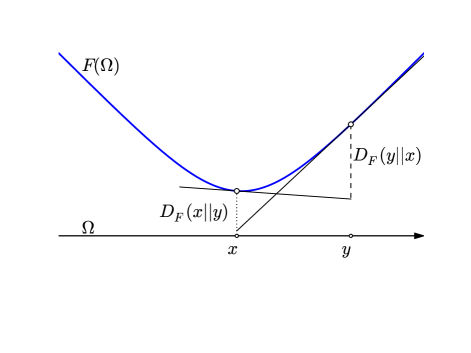
Figure 1. Geometric interpretation of the Bregman divergence associated with the function ${{F}}$ on ${\Omega}$.

Accordingly, we introduce two balls of radius $r\geq 0$ centered at a point $x\in{\Omega}$: the primal Bregman ball containing all points $y$ so that the divergence from $x$ to $y$ is at most $r$, and the dual Bregman ball containing all points $y$ so that the divergence from $y$ to $x$ as at most $r$:

$${B}_{{{{F}}}}{({x};{r})} =\{y\in{\Omega}\mid{{D}_{{{F}}}{({x}\|{y})}}\leq r\};$$ (2)

$${B}_{{{{F}}}}^{\prime}{({x};{r})} =\{y\in{\Omega}\mid{{D}_{{{F}}}{({y}\|{x})}}\leq r\}.$$ (3)

To construct the primal ball geometrically, we take the point $(x,{{F}}(x)-r)$ at height $r$ below the graph of ${{F}}$ and shine light along straight half-lines emanating from this point onto the graph. The ball is the vertical projection of the illuminated portion onto ${\mathbb{R}}^{n}$; see Figure 2. To construct the dual ball geometrically, we start with the hyperplane that touches the graph of ${{F}}$ at $(x,{{F}}(x))$, translating it to height $r$ above the initial position. The ball is the vertical projection of the portion of the graph below the translated hyperplane onto ${\mathbb{R}}^{n}$; see again Figure 2.

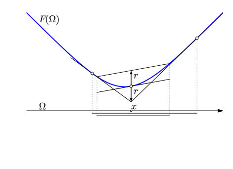
Figure 2. The primal Bregman ball with center $x$ is obtained by illuminating the graph of ${{F}}$ from below. In contrast, the dual Bregman ball is constructed by cutting the graph with the elevated line.

Since ${{D}_{{{F}}}}$ is not necessarily symmetric, the two Bregman balls are not necessarily the same. Indeed, the dual ball is necessarily convex while the primal ball is not.

1Convexity Property.

${{D}_{{{F}}}}\colon{\Omega}\times{\Omega}\to{\mathbb{R}}$ is strictly convex in the first argument but not necessarily convex in the second argument.

Proof.

Fixing $y$, set $f(x)={{D}_{{{F}}}{({x}\|{y})}}$. According to (1), $f$ is the difference between ${{F}}$ and an affine function; compare with the geometric interpretation of the dual Bregman ball. The strict convexity of ${{F}}$ implies the strict convexity of $f$. This argument does not apply to $g(y)={{D}_{{{F}}}{({x}\|{y})}}$, which we obtain by fixing $x$, and it is easy to find an example in which $g$ is non-convex; see Figure 4.

Legendre transform and conjugate function.

In a nutshell, the Legendre transform applies elementary polarity to the graph of ${{F}}$, giving rise to the graph of another, conjugate function, ${{F}}^{*}\colon{\Omega}^{*}\to{\mathbb{R}}$, that relates to ${{F}}$ in interesting ways. If ${{F}}$ is of Legendre type then so is ${{F}}^{*}$; see [31, Theorem 26.5].

The notion of polarity we use in this paper relates points in ${\mathbb{R}}^{n}\times{\mathbb{R}}$ with affine functions ${\mathbb{R}}^{n}\to{\mathbb{R}}$. Specifically, it maps a point $C=(c,\gamma)$ to the function defined by $C^{*}(x)={\langle c,x\rangle}-\gamma$, and it maps $C^{*}$ back to $(C^{*})^{*}=C$. We refer to Figure 3 for an illustration and to Appendix A for more details.

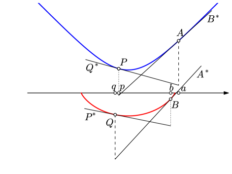
Figure 3. Top: the graph of ${{F}}$ and the tangent lines that illustrate the two Bregman divergences between $a$ and $p$ associated with ${{F}}$. Bottom: the graph of ${{F}}^{*}$ and the tangent lines that illustrate the two Bregman divergences between $b=a^{*}$ and $q=p^{*}$ associated with ${{F}}^{*}$.

As a first step in constructing the conjugate function, we get ${\Omega}^{*}$ as the set of points $e=c^{*}=\nabla{{F}}(c)$ with $c\in{\Omega}$. We define $h\colon{\Omega}\to{\Omega}^{*}$ by mapping $c$ to $h(c)=c^{*}$. Note that differentiability of strictly convex functions implies continuous differentiability [14, Theorem 2.86], hence $h$ is a homeomorphism between the two domains.

The conjugate function, ${{F}}^{*}\colon{\Omega}^{*}\to{\mathbb{R}}$, is then defined by mapping $e$ to ${{F}}^{*}(e)=\epsilon$ such that $(e,\epsilon)$ is the polar point of the affine function whose graph touches the graph of ${{F}}$ in the point $(c,{{F}}(c))$. Writing $b=a^{*}$ and $q=p^{*}$, we get

$${D}_{{{F}}^{*}}{({b}\|{q})} ={{F}}^{*}(b)-P^{*}(b)\geq 0,$$ (4)

$${D}_{{{F}}^{*}}{({q}\|{b})} ={{F}}^{*}(q)-A^{*}(q)\geq 0$$ (5)

from (22), (22) and (26), (27) in Appendix A; see again Figure 3. The left-hand sides of (4) and (5) are both non-negative and vanish iff $b=q$. Since this is true for all points $b,q\in{\Omega}^{*}$, ${{F}}^{*}$ is strictly convex, provided ${\Omega}^{*}$ is convex. Proving that this assumption is always fulfilled is more involved. We therefore resort to a classical theorem [31, Theorem 26.5], which states that ${{F}}^{*}$ is again of Legendre type and, in particular, ${\Omega}^{*}$ is convex. Hence, ${{F}}^{*}$ defines a Bregman divergence and, importantly, this divergence is symmetric to the one defined by ${{F}}$.

2Duality Property.

Let ${{F}}\colon{\Omega}\to{\mathbb{R}}$ and ${{F}}^{*}\colon{\Omega}^{*}\to{\mathbb{R}}$ be conjugate functions of Legendre type. Then ${{D}_{{{F}}}{({a}\|{p})}}={{D}_{{{F}}^{*}}{({p^{*}}\|{a^{*}})}}$ for all $a,p\in{\Omega}$.

In words, the Legendre transform preserves the divergences, but it does so by exchanging the arguments. This is interesting because ${{D}_{{{F}}}}$ is strictly convex in the first argument and so is ${{D}_{{{F}}^{*}}}$, only that its first argument corresponds to the second argument of ${{D}_{{{F}}}}$. To avoid potential confusion, we thus consider the primal and dual Bregman balls of ${{F}}^{*}$:

$${B}_{{{{F}}^{*}}}{({u};{r})} =\{v\in{\Omega}^{*}\mid{{D}_{{{F}}^{*}}{({u}\|{v})}}\leq r\},$$ (6)

$${B}_{{{{F}}^{*}}}^{\prime}{({u};{r})} =\{v\in{\Omega}^{*}\mid{{D}_{{{F}}^{*}}{({v}\|{u})}}\leq r\},$$ (7)

where we write $u=x^{*}$ and $v=y^{*}$ so we can compare the two balls with the ones defined in (2) and (3). As mentioned earlier, both dual balls are necessarily convex while both primal balls are possibly non-convex. Recall the homeomorphism $h\colon{\Omega}\to{\Omega}^{*}$ that maps $x$ to $x^{*}$. It also maps ${{B}_{{{{F}}}}{({x};{r})}}$ to ${{B}_{{{{F}}^{*}}}^{\prime}{({u};{r})}}$ and ${{B}_{{{{F}}}}^{\prime}{({x};{r})}}$ to ${{B}_{{{{F}}^{*}}}{({u};{r})}}$. In words, it makes the non-convex ball convex and the convex ball non-convex, and it does this while preserving the divergences. We use this property to explain the necessity on using functions of Legendre type; it also plays a crucial role later. Consider a dual Bregman ball with a non-convex conjugate image, namely the corresponding primal ball. Then the restriction of ${{F}}$ to this dual ball is strictly convex and differentiable. However, it is not of Legendre type and its conjugate has a non-convex domain.

Examples.

We close this section with a short list of functions, their conjugates, and the corresponding Bregman divergences. Half the squared Euclidean norm maps a point $x\in{\mathbb{R}}^{n}$ to ${{F}}(x)=\tfrac{1}{2}{\|{x}\|}^{2}$. The gradient is $\nabla{{F}}(x)=x$, and the conjugate is defined by ${{F}}^{*}(x)={{F}}(x)$. The divergence associated with ${{F}}$ is half the squared Euclidean distance:

$${D}_{{{F}}}{({x}\|{y})} =\tfrac{1}{2}{\|{x}-{y}\|}^{2}.$$ (8)

This Bregman divergence is special because it is symmetric in the two arguments.

The Shannon entropy of a discrete probability distribution is $-\sum_{i=1}^{n}x_{i}\ln x_{i}$. To turn this into a convex function, we change the sign, and to simplify the computations, we subtract the sum of the $x_{i}$, defining ${{F}}(x)=\sum_{i=1}^{n}[x_{i}\ln x_{i}-x_{i}]$ over the positive orthant, which we denote as ${\mathbb{R}}^{n}_{+}$. The gradient is $\nabla{{F}}(x)=[\ln x_{1},\ln x_{2},\ldots,\ln x_{n}]^{T}$, and the conjugate is the exponential function, ${{F}}^{*}(u)=\sum_{i=1}^{n}e^{u_{i}}$, with $u=x^{*}$, defined on ${\mathbb{R}}^{n}$. Associated with ${{F}}$ is the Kullback–Leibler divergence and with ${{F}}^{*}$ is the exponential loss:

$${D}_{{{F}}}{({x}\|{y})} =\sum_{i=1}^{n}\left[x_{i}\ln\tfrac{x_{i}}{y_{i}}-x_{i}+y_{i}\right],$$ (9)

$${D}_{{{F}}^{*}}{({u}\|{v})} =\sum_{i=1}^{n}\left[e^{u_{i}}-(u_{i}-v_{i}+1)e^{v_{i}}\right].$$ (10)

The Kullback–Leibler is perhaps the best known Bregman divergence; it is also referred to as the information divergence, information gain, relative entropy; see [2, page 57]. If applied to finite distributions, ${{F}}$ would be defined on the standard $(n-1)$-simplex, where it measures the difference in information when we go from $y$ to $x$. It also measures the expected number of extra bits required to code samples from $x$ using a code that is optimized for $y$ instead of for $x$. Since the $(n-1)$-simplex is the intersection of ${\mathbb{R}}^{n}_{+}$ with a hyperplane, this restriction of ${{F}}$ is again of Legendre type. In this particular case, we can extend the function to the closed $(n-1)$-simplex, so that some coordinates may be zero, provided we accept infinite divergences for some pairs. In other words, the framework is also suitable for sparse data, pervasive for example in text-retrieval applications.

The Burg entropy maps a point $x\in{\mathbb{R}}^{n}_{+}$ to ${{F}}(x)=\sum_{i=1}^{n}[1-\ln x_{i}]$. The components of the gradient are $-1/x_{i}$, for $1\leq i\leq n$. The conjugate is the function ${{F}}^{*}\colon{\mathbb{R}}^{n}_{-}\to{\mathbb{R}}$ defined by ${{F}}^{*}(u)=\sum_{i=1}^{n}\left[1-\ln|u_{i}|\right]$. Associated with ${{F}}$ is the Itakura–Saito divergence:

$${D}_{{{F}}}{({x}\|{y})} =\sum_{i=1}^{n}\left[\tfrac{x_{i}}{y_{i}}-\ln\tfrac{x_{i}}{y_{i}}-1\right].$$ (11)

We note that ${{F}}$ and ${{F}}^{*}$ are very similar, but their domains are diagonally opposite orthants. Indeed, the Itakura–Saito distance is not symmetric and generates non-convex primal balls; see Figure 4.

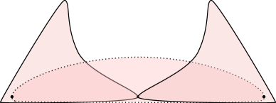
Figure 4. Two primal Itakura–Saito balls and the dual Itakura–Saito ball centered at the point where the primal balls touch. Its boundary passes through the centers of the primal balls.

3. Proximity Complexes for Bregman divergences

In this section, we extend the standard constructions of topological data analysis (Čech, Vietoris–Rips, Delaunay complexes) to the setting of Bregman divergences. Importantly, we prove the contractibility of non-empty common intersections of Bregman balls and Voronoi domains. This property guarantees that the Čech and Delaunay complexes capture the correct homotopy type of the data.

Contractibility for balls.

Every non-empty convex set is contractible, which means it has the homotopy type of a point. The common intersection of two or more convex sets is either empty or again convex and therefore contractible. While primal Bregman balls are not necessarily convex, we show that their common intersections are contractible unless empty. The reason for our interest in this property is the Nerve Theorem [8, 25], which asserts that the nerve of a cover with said property has the same homotopy type as the union of this cover.

3Contractibility Lemma for Balls.

Let ${{F}}\colon{\Omega}\to{\mathbb{R}}$ be of Legendre type, $X\subseteq{\Omega}$, and $r\geq 0$. Then $\bigcap_{x\in X}{{B}_{{{{F}}}}{({x};{r})}}$ is either empty or contractible.

Proof.

Recall the homeomorphism $h\colon{\Omega}\to{\Omega}^{*}$ obtained as a side-effect of applying the Legendre transform to ${{F}}$. It maps every primal Bregman ball in ${\Omega}$ homeomorphically to a dual Bregman ball in ${\Omega}^{*}$, which is convex. Similarly, it maps the common intersection of primal Bregman balls in ${\Omega}$ homeomorphically to the common intersection of dual Bregman balls in ${\Omega}^{*}$: $h({\mathbb{X}})={\mathbb{Y}}$ in which ${\mathbb{X}}=\bigcap_{x\in X}{{B}_{{{{F}}}}{({x};{r})}}$ and ${\mathbb{Y}}=\bigcap_{x\in X}{{B}_{{{{F}}^{*}}}^{\prime}{({x^{*}};{r})}}$. Since ${\mathbb{X}}$ and ${\mathbb{Y}}$ are homeomorphic, they have the same homotopy type. Hence, either ${\mathbb{X}}={\mathbb{Y}}=\emptyset$ or ${\mathbb{Y}}$ is convex and ${\mathbb{X}}$ is contractible.

Čech and Vietoris–Rips constructions for Bregman divergences.

The contractibility of the common intersection suggests we take the nerve of the Bregman balls. Given a finite set $X\subseteq{\Omega}$ and $r\geq 0$, we call the resulting simplicial complex the Čech complex of $X$ and $r$ associated with ${{F}}$. Related to it is the Vietoris–Rips complex, which is the clique complex of the $1$-skeleton of the Čech complex:

$${\mbox{$\rm\check{C}ech$}}_{{{{F}}}}{({X};{r})} =\{P\subseteq X\mid\bigcap_{p\in P}{{B}_{{{{F}}}}{({p};{r})}}\neq\emptyset\},$$ (12)

$${\mbox{$\rm Rips$}}_{{{{F}}}}{({X};{r})} =\{Q\subseteq X\mid\tbinom{Q}{2}\subseteq{\rm\check{C}ech}_{{{{F}}}}{({X};{r})}\}.$$ (13)

In words, the Vietoris–Rips complex contains a simplex iff all its edges belong to the Čech complex. We note that for ${{F}}(x)={\|{x}\|}^{2}$, (13) translates to the usual Euclidean definition of the Vietoris–Rips complex. Increasing the radius from $0$ to $\infty$, we get a filtration of Čech complexes and a filtration of Vietoris–Rips complexes. By construction, the Čech complex is contained in the Vietoris–Rips complex for the same radius. If we measure distance with the Euclidean metric, this relation extends to

$${\mbox{$\rm\check{C}ech$}}{({X};{r})}\subseteq{\rm Rips}{({X};{r})}\subseteq{\rm\check{C}ech}{({X};{\sqrt{2}r})}.$$ (14)

Indeed, if all pairs in a set of $k+1$ balls of radius $r$ have a non-empty common intersection, then increasing the radius to $\sqrt{2}r$ guarantees that the $k+1$ balls have a non-empty intersection. This fact is often expressed by saying that the two filtrations have a small interleaving distance if indexed logarithmically.

No interleaving.

The interleaving property expressed in (14) extends to general metrics – except that the constant factor is $2$ rather than $\sqrt{2}$ – but not to general Bregman divergences. To see that (14) does not extend, we give an example of $3$ points whose Bregman balls overlap pairwise for a small radius but not triplewise until the radius is very large.

The example uses the exponential function defined on the standard triangle, which we parametrize using barycentric coordinates. For convenience, the explanation uses the conjugate function, which is the Shannon entropy; that is: we look at dual balls in which distance is measured with the Kullback–Leibler divergence. Specifically, we use ${{F}}(x)=\sum_{i=1}^{3}x_{i}\ln x_{i}$. The barycentric coordinates are non-negative and satisfy $\sum_{i=1}^{3}x_{i}=1$. We therefore get the maximum value of $0$ at the three corners, and the minimum of $-\ln 3$ at the center of the triangle; see Figure 5. After some calculations, we get the squared length of the gradient at $x$ as $\tfrac{1}{3}[(\ln x_{1}-\ln x_{2})^{2}+(\ln x_{1}-\ln x_{3})^{2}+(\ln x_{2}-\ln x_{3})^{2}]$. It goes to infinity when $x$ approaches the boundary of the triangle.

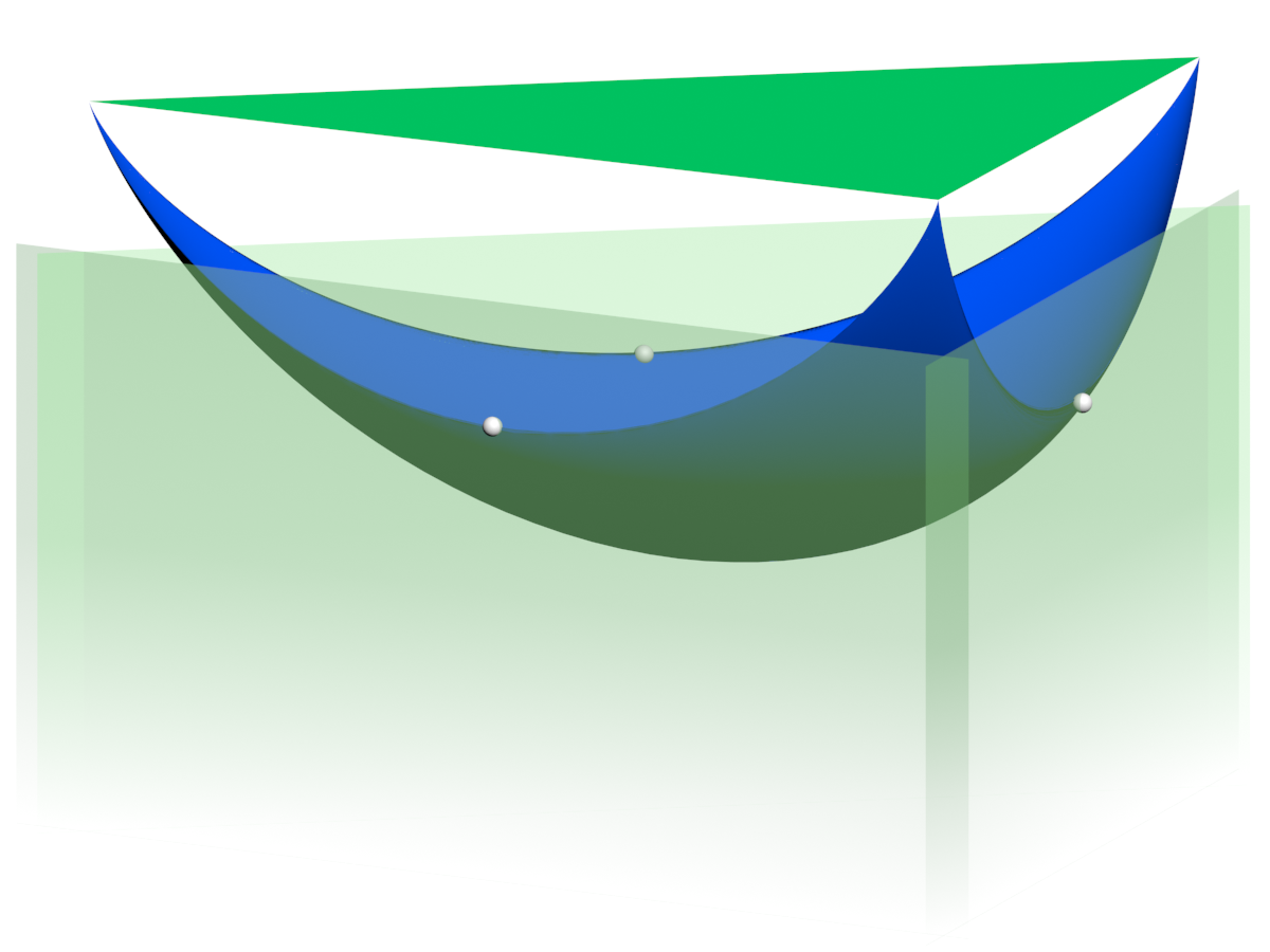
Figure 5. Three points for which pairwise intersecting dual Kullback–Leibler balls centered at these points can be small, but triplewise intersecting such balls are necessarily large.

We construct the example using points near the midpoints of the edges. Choosing them in the interior of the triangle but close to the boundary, the corresponding three tangent planes are as steep as we like. Moving the planes upward, we get the dual balls as the vertical projections of the parts of the graph of ${{F}}$ on or below the planes. Moving the planes continuously, we let $r$ be the height above the initial positions, and note that $r$ is also the radius of the dual balls. Pairwise overlap between the balls starts when the three lines at which the planes meet intersect the graph of ${{F}}$. This happens at $r<\ln 3$. Triplewise overlap starts when the point common to all three planes passes through the graph of ${{F}}$. This happens at a value of $r$ that we can make arbitrarily large.

Contractibility for Voronoi domains.

Čech and Vietoris–Rips complexes can be high-dimensional and of exponential size, even if the data lives in low dimensions. To remedy this shortcoming, we use the Delaunay (or alpha) complex; see [17, 18]. It is obtained by clipping the balls before taking the nerve. We explain this by introducing the Voronoi domains of the generating points as the clipping agents. Letting $X\subseteq{\Omega}$ be finite, we define the primal and dual Voronoi domains of $x\in X$ associated with ${{F}}$ as the sets of points for which $x$ minimizes the Bregman divergence to or from the point:

$${V}_{\!{{F}}}{({x})} =\{a\in{\Omega}\mid{{D}_{{{F}}}{({x}\|{a})}}\leq{{D}_{{{F}}}{({y}\|{a})}},\forall y\in X\};$$ (15)

$${V}_{{{F}}}^{\prime}{({x})} =\{a\in{\Omega}\mid{{D}_{{{F}}}{({a}\|{x})}}\leq{{D}_{{{F}}}{({a}\|{y})}},\forall y\in X\}.$$ (16)

An intuitive construction of the primal domains grows the primal Bregman balls around the points, stopping the growth at places where the balls meet. Similarly, we get the dual Voronoi domains by growing dual Bregman balls. Not surprisingly, the primal Voronoi domains are not necessarily convex, and the dual Voronoi cells are convex. To see the latter property, we recall that the dual ball centered at $x$ is constructed by translating the hyperplane that touches the graph of ${{F}}$ above $x$. Specifically, ${{D}_{{{F}}}{({a}\|{x})}}$ is the height at which the hyperplane passes through the point $(a,{{F}}(a))$. This implies that we can construct the dual Voronoi domains as follows:

• For each $x\in X$, consider the half-space of points in ${\mathbb{R}}^{n}\times{\mathbb{R}}$ on or above the hyperplane that touches the graph of ${{F}}$ at $(x,{{F}}(x))$.

• Form the intersection of these half-spaces, which is a convex polyhedron. We call its boundary the upper envelope of the hyperplanes, noting that it is the graph of a piecewise linear function from ${\mathbb{R}}^{n}$ to ${\mathbb{R}}$.

• Project the upper envelope vertically onto ${\mathbb{R}}^{n}$. Each dual Voronoi domain is the intersection of ${\Omega}$ with the image of an $n$-dimensional face of the upper envelope.

We conclude that the dual Voronoi domains are convex and use this property to show that the primal Voronoi domains intersect contractibly.

4Contractibility Lemma for Voronoi Domains.

Let ${{F}}\colon{\Omega}\to{\mathbb{R}}$ be of Legendre type, and $X\subseteq{\Omega}$ finite. Then $\bigcap_{x\in X}{{V}_{\!{{F}}}{({x})}}$ is either empty or contractible.

The proof is similar to that of the Contractibility Lemma for Balls and therefore omitted.

Delaunay construction for Bregman divergences.

Taking the nerve of the primal Voronoi domains, we get the Delaunay triangulation of $X$ associated with ${{F}}$, which we denote as ${\rm Del}_{{{F}}}{({X})}$. Further restricting the primal Voronoi domains by primal Bregman balls of radius $r$, we get the Delaunay complex of $X$ and $r$ associated with ${{F}}$:

$$\!\!{\rm Del}_{{{{F}}}}{({X};{r})} =\{P\!\subseteq\!X\mid\!\bigcap_{p\in P}\!\left[{{B}_{{{{F}}}}{({p};{\!r})}}\cap{{V}_{\!{{F}}}{({p})}}\right]\neq\emptyset\}.$$ (17)

Assuming general position of the points in $X$, the Delaunay triangulation is a simplicial complex of dimension at most $n$. We will be explicit about what we mean by general position shortly. Combining the proofs of the two Contractibility Lemmas, we see that the common intersection of any set of clipped primary balls is either empty or contractible. This together with the Nerve Theorem implies that ${\rm Del}_{{{{F}}}}{({X};{r})}$ has the same homotopy type as ${\rm\check{C}ech}_{{{{F}}}}{({X};{r})}$, namely the homotopy type of the union of the Bregman balls that define the two complexes.

4. Algorithms

Recall that all three proximity complexes defined in Section 3 depend on a radius parameter. In this section, we give algorithms that compute the values of this parameter beyond which the simplices belong to the complexes. By focusing on the resulting radius functions, we decouple the computation of the radius for each simplex from the technicalities of constructing the actual simplicial complex. In particular, we show that the Čech complexes can be efficiently reconstructed from the Vietoris–Rips complexes, and the Delaunay complexes from the Delaunay triangulations. We exploit a connection with discrete Morse theory to develop efficient algorithms.

Radius functions.

Let $X\subseteq{\Omega}$ be finite, write $\Delta(X)$ for the simplex whose vertices are the points in $X$, and recall that ${\rm Del}_{{{F}}}{({X})}$ is the Delaunay triangulation of $X$ associated with ${{F}}$. The Čech, Vietoris–Rips, and Delaunay radius functions associated with ${{F}}$,

$$\varrho_{{{F}}}^{\rm\check{C}ech} \colon\Delta(X)\to{\mathbb{R}},$$ (18)

$$\varrho_{{{F}}}^{\rm Rips} \colon\Delta(X)\to{\mathbb{R}},$$ (19)

$$\varrho_{{{F}}}^{\rm Del} \colon{\rm Del}_{{{F}}}{({X})}\to{\mathbb{R}},$$ (20)

are defined such that $P\in{\rm\check{C}ech}_{{{{F}}}}{({X};{r})}$ iff ${\varrho_{{{F}}}^{\rm\check{C}ech}}(P)\leq r$, and similarly for Vietoris–Rips and for Delaunay. By definition of the Čech complex, ${\varrho_{{{F}}}^{\rm\check{C}ech}}(P)$ is the minimum radius at which the primal Bregman balls centered at the points of $P$ have a non-empty common intersection. We are interested in an equivalent characterization using dual Bregman balls. To this end, we say that a dual Bregman ball, ${{B}^{\prime}}$, includes $P$ if $P\subseteq{{B}^{\prime}}$, and we call ${{B}^{\prime}}$ the smallest including dual ball if there is no other dual ball that includes $P$ and has a smaller radius. Because ${{F}}$ is strictly convex, the smallest including dual ball of $P$ is unique; see Figure 4, which shows the smallest including dual Itakura–Saito ball of a pair of points. We call ${{B}^{\prime}}$ empty if no point of $X$ lies in its interior, and we call it a circumball of $P$ if all points of $P$ lie on its boundary. We observe that a simplex $P\in\Delta(X)$ belongs to ${\rm Del}_{{{F}}}{({X})}$ iff it has an empty dual circumball. Because ${{F}}$ is strictly convex, the smallest empty dual circumball of a simplex is either unique or does not exist. The characterization of the radius functions in terms of dual balls is strictly analogous to the Euclidean case studied in [4].

5Radius Function Lemma.

Let ${{F}}\colon{\Omega}\to{\mathbb{R}}$ be of Legendre type, $X\subseteq{\Omega}$ finite, and $\emptyset\neq P\subseteq X$.

1. ${\varrho_{{{F}}}^{\rm\check{C}ech}}(P)$ is the radius of the smallest including dual ball of $P$, and ${\varrho_{{{F}}}^{\rm Rips}}(P)$ is the maximum radius of the smallest including dual balls of the pairs in $P$.

2. Assuming $P\in{\rm Del}_{{{F}}}{({X})}$, ${\varrho_{{{F}}}^{\rm Del}}(P)$ is the radius of the smallest empty dual circumball of $P$.

We omit the proof, which is not difficult. Every circumball also includes, which implies ${\varrho_{{{F}}}^{\rm Rips}}(P)\leq{\varrho_{{{F}}}^{\rm\check{C}ech}}(P)\leq{\varrho_{{{F}}}^{\rm Del}}(P)$ whenever the radius functions are defined. Correspondingly, ${\rm Del}_{{{{F}}}}{({X};{r})}\subseteq{\rm\check{C}ech}_{{{{F}}}}{({X};{r})}\subseteq{\rm Rips}_{{{{F}}}}{({X};{r})}$ for every value of $r$.

General position.

It is often convenient and sometimes necessary to assume that the points in $X\subseteq{\Omega}$ are in general position, for example when we require the Delaunay triangulation be a simplicial complex in ${\mathbb{R}}^{n}$. Here is a notion that suffices for the purposes of this paper.

6Definition of General Position.

Let ${\Omega}\subseteq{\mathbb{R}}^{n}$ and ${{F}}\colon{\Omega}\to{\mathbb{R}}$ of Legendre type. A finite set $X\subseteq{\Omega}$ is in general position with respect to ${{F}}$ if, for every $P\subseteq X$ of cardinality at most $n+1$,

1. the points in $P$ are affinely independent,

2. no point of $X\setminus P$ lies on the boundary of the smallest dual circumball of $P$.

Let $k={\rm dim}\,{P}$. Property I implies that $P$ has an $(n-k)$-parameter family of circumballs. In particular, there is at least one circumball as long as $k\leq n$. Property II implies that no two different simplices have the same smallest dual circumball. In particular, no two $n$-simplices in the Delaunay triangulation have the same circumball.

Discrete Morse theory.

For points in general position, two of the radius functions exhibit a structural property that arises in the translation of Morse theoretic ideas from the smooth category to the simplicial category. Following [4], we extend the original formulation of discrete Morse theory given by Forman [20]. Letting $K$ be a simplicial complex, and $P,R\in K$ two simplices, we write $P\leq R$ if $P$ is a face of $R$. The interval of simplices between $P$ and $R$ is $[P,R]=\{Q\in K\mid P\leq Q\leq R\}$. We call $P$ the lower bound and $R$ the upper bound of the interval. A generalized discrete vector field is a partition of $K$ into intervals. We call it a generalized discrete gradient if there exists a function $f\colon K\to{\mathbb{R}}$ such that $f(P)\leq f(Q)$ whenever $P$ is a face of $Q$, with equality iff $P$ and $Q$ belong to a common interval. A function with this property is called a generalized discrete Morse function. To get an intuitive feeling for this concept, consider the sequence of sublevel sets of $f$. Any two contiguous sublevel sets differ by one or more intervals, and any two of these intervals are independent in the sense that neither interval contains a face of a simplex in the other interval. Indeed, this property characterizes generalized discrete Morse functions.

7GDMF Theorem.

Let ${{F}}\colon{\Omega}\to{\mathbb{R}}$ be of Legendre type and let $X\subseteq{\Omega}$ be finite and in general position. Then ${\varrho_{{{F}}}^{\rm\check{C}ech}}\colon\Delta(X)\to{\mathbb{R}}$ and ${\varrho_{{{F}}}^{\rm Del}}\colon{\rm Del}_{{{F}}}{({X})}\to{\mathbb{R}}$ are generalized discrete Morse functions.

We give the proof in Appendix B. Observe that the Vietoris–Rips radius function is not a generalized discrete Morse function. The structural properties implied by the GDMF Theorem will be useful in the design of algorithms that compute the radius functions. The theorem should be compared with the analogous result in the Euclidean case [4]. The arguments used there can be translated almost verbatim to prove additional structural results for Bregman divergences. Perhaps most importantly, they imply that the Wrap complex of ${{F}}$ and $X$ is well defined – see [16] for the original paper on these complexes defined in $3$-dimensional Euclidean space – and that the Čech complex collapses to the Delaunay complex and further to the Wrap complex, all defined for the same radius.

Bregman circumball algorithm.

Depending on how the function ${{F}}$ is represented, there may be a numerical component to the algorithms needed to find smallest including dual balls. Consider a $k$-simplex $Q\subseteq X$ with $0\leq k\leq n$. Assuming general position, the affine hull of the points $A=(a,{{F}}(a))$ with $a\in Q$ is a $k$-dimensional plane, which we denote as ${\cal Q}$. We are interested in the point $(q,\psi)\in{\cal Q}$ that maximizes $\psi-{{F}}(q)$, the height above the graph of ${{F}}$. The point $q$ is the center of the smallest dual circumball of $Q$, and $\psi-{{F}}(q)$ is the radius. Interestingly, this observation implies that the point of first intersection of two primal Bregman balls lies on a line joining their centers. For later reference, we assume a routine that computes this point, possibly using a standard numerical optimization method.

dualball routine CircumBall $(Q)$:
	let ${\cal Q}$ be the affine hull of the points $(a,{{F}}(a))$, $a\in Q$;
	find $(q,\psi)\in{\cal Q}$ maximizing $\psi-{{F}}(q)$;
	return $(q,\psi-{{F}}(q))$.

This is an unconstrained $k$-dimensional convex optimization, and $k$ is much smaller than $n$ for high dimensional data. Indeed, the optimization can be performed in the space of affine coordinates of the plane ${\cal Q}$. Importantly, the Hessian is of dimension $k\times k$ and not $n\times n$, which would be prohibitive. This allows us to use second-order quasi-Newton methods, such as the fast BFGS algorithm [28].

Note that the smallest dual circumball of $Q$ includes $Q$ but is not necessarily the smallest including dual ball. However, the latter is necessarily the smallest dual circumball of a face of $Q$. Next, we show how the CircumBall routine is used to efficiently compute the radius functions.

Čech radius function algorithm.

According to the Radius Function Lemma (i), the value of a simplex, $Q\in\Delta(X)$, under the Čech radius function is the radius of the smallest including dual ball of $Q$. To compute this value, we visit the simplices in a particular sequence. Recalling the GDMF Theorem, we note that the smallest including dual ball of a simplex $Q$ is the smallest dual circumball of the minimum face $P\subseteq Q$ in the same interval. It is therefore opportune to traverse the simplices in the order of increasing dimension. Whenever the smallest dual circumball of a simplex $Q$ is not the smallest including dual ball, we get ${\varrho_{{{F}}}^{\rm\check{C}ech}}(Q)$ from one of its codimension $1$ faces. We identify such a simplex $Q$ when we come across a face whose smallest dual circumball includes $Q$, and we mark $Q$ with the center and radius of this ball. The following pseudocode computes the radius function of the Čech complex restricted to the $k$-skeleton of $\Delta(X)$ for some nonnegative integer $k$:

for $i=0$ to $k$ do
	forall $P\subseteq X$ with ${\rm dim}\,{P}=i$ do
		if $P$ unmarked then $(p,r)=\mbox{\sc CircumBall}(P)$;
		forall $a\in X$ with ${{D}_{F}{({a}\|{p})}}<r$ do mark $P\cup\{a\}$ with $(p,r)$.

As in the Euclidean setting, the size of $\Delta(X)$ is exponential in the size of $X$ so that the computations are feasible only for reasonably small values of $k$ or small radius cut-offs. In practice, we would run the algorithm with a radius cut-off, or use an approximation strategy yielding a similar persistence diagram.

Observe the similarity to the standard algorithm for constructing the $k$-skeleton of the Vietoris–Rips complex: after adding all edges of length at most $2r$, we add simplices of dimension $2$ and higher whenever possible. Geometric considerations are thus restricted to edges and the rest of the construction is combinatorial; see [34] for a fast implementation. Our algorithm can be interpreted as constructing the Čech complex from the Vietoris–Rips complex at the cost of at most one call to CircumBall per simplex. This is more efficient than explicitly computing the smallest including dual ball for each simplex, even if we use fast randomized algorithms as described in [27, 33]. Furthermore, the CircumBall routine is only called for the lower bounds of the intervals of the Čech radius function or, equivalently, for each subcomplex in the resulting filtration. The number of such intervals depends on the relative position of the points in $X$ and not only on the cardinality. Notwithstanding, the number of intervals is significantly smaller than the number of simplices in the Čech complex. This suggests that only a small overhead is needed to compute the Čech from the Vietoris–Rips complexes. Our preliminary experiments for the Kullback-Leibler divergence support this claim; see Table 1. Note that the number of calls to the CircumBall routine is between $\frac{1}{10}$ and $\frac{1}{3}$ of the number of simplices, with an average between $6$ and $15$ function evaluations per call.

Table 1. Experimental evaluation on three synthetic datasets: (A) Full Čech complex with 20 points in ${\mathbb{R}}^{20}$; (B) $3$-skeleton with 256 points in ${\mathbb{R}}^{4}$ and radius cutoff $r=0.1$; (C) $4$-skeleton with 4,000 points in ${\mathbb{R}}^{4}$ and radius cutoff $r=0.01$.

	A (20 pts)	B (256 pts)	C (4,000 pts)
#edges	190	7,715	36,937
#simplices	1,048,575	1,155,301	1,222,688
#calls to CircumBall	104,030	346,475	283,622
#function evaluations in CircumBall	1,523,295	2,904,603	1,783,474

Delaunay radius function algorithm.

According to the Radius Function Lemma (ii), the value of a simplex $Q\in{\rm Del}_{{{F}}}{({X})}$ under the Delaunay radius function is the radius of the smallest empty dual Bregman circumball of $Q$.

real routine DelaunayRadius $(Q)$:
	$(q,r)=\mbox{\sc CircumBall}(Q)$;
	forall $a\in X\setminus Q$ do
		if ${{D}_{{{F}}}{({a}\|{q})}}<r$ then return none;
	return $r$.

The CircumBall routine gives only the smallest dual circumball of $Q$, and if it is not empty, then we have to get the value of the Delaunay radius function from somewhere else. According to the GDMF Theorem, we get the value from the maximum simplex in the interval that contains $Q$. It is therefore opportune to traverse the simplices of the Delaunay triangulation in the order of decreasing dimension. Whenever the smallest dual circumball of a simplex $Q$ is non-empty, we get ${\varrho_{{{F}}}^{\rm Del}}(Q)$ from one of the simplices that contain $Q$ as a codimension $1$ face.

As already observed in [7], we can construct the full Delaunay triangulation, ${\rm Del}_{{{F}}}{({X})}$, using existing algorithms for the Euclidean case. We get the Delaunay complexes as sublevel sets of the radius function. Specifically, we first use the polarity transform to map the points $(x,{{F}}(x))$ to the corresponding affine functions; see Section 2. We then get a geometric realization of ${\rm Del}_{{{F}}}{({X})}$ from the vertical projection of the upper envelope of the affine functions onto ${\mathbb{R}}^{n}$, which is a Euclidean weighted Voronoi diagram, also known as power diagram or Dirichlet tessellation. Its dual is the Euclidean weighted Delaunay triangulation, also known as regular or coherent triangulation. The data that defines these Euclidean diagrams are the points $x\in X$ with weights $\xi={{F}}(x)-{\|{x}\|}^{2}$. Finally, after computing the radius function on all simplices in ${\rm Del}_{{{F}}}{({X})}$, we get the Delaunay complexes as a filtration of this weighted Delaunay triangulation. Interestingly, this is not necessarily the filtration we obtain by simultaneously and uniformly increasing the weights of the points.

5. Discussion

The main contribution of this paper is the extension of the mathematical and computational machinery of topological data analysis (TDA) to applications in which distance is measured with a Bregman divergence. This includes text and image data often compared with the Kullback–Leibler divergence, and speech and sound data often studied with the Itakura–Saito divergence. It is our hope that the combination of Bregman divergences and TDA technology will bring light into the generally difficult study of high-dimensional data. In support of this optimism, Rieck and Leitte [30] provide experimental evidence that good dimension reduction methods preserve the persistent homology of the data. With our extension to Bregman divergences, such experiments can now be performed for a much wider spectrum of applications. There are specific mathematical questions whose incomplete understanding is currently an obstacle to progress in the direction suggested by this paper:

• A cornerstone of TDA is the stability of its persistence diagrams, as originally proved in [13]. How does the use of Bregman divergences affect the stability of the diagrams?

• Related to the question of stability is the existence of sparse complexes and filtrations for data in Bregman spaces whose persistence diagrams are close to the ones we get for the Čech and Delaunay complexes.

Last but not least, we mention the urgent task to further study the related algorithmic questions and to implement software that is fast, can cope with large sets of data, and is easy to use also for non-specialists.

Acknowledgements

The authors thank Žiga Virk for discussions on the material presented in this paper.

Appendix A Polarity and Legendre Transform

In this appendix, we give further details how the polarity transform amounts to the Legendre transform for functions of Legendre type. Recall that the polarity maps a point $C=(c,\gamma)\in{\mathbb{R}}^{n}\times{\mathbb{R}}$ to the function $C^{*}\colon{\mathbb{R}}^{n}\to{\mathbb{R}}$ defined by $C^{*}(x)={\langle c,x\rangle}-\gamma$, and that it maps $C^{*}$ back to $(C^{*})^{*}=C$. Given a second point $S=(s,\sigma)\in{\mathbb{R}}^{n}\times{\mathbb{R}}$, and the corresponding affine function $S^{*}(x)={\langle s,x\rangle}-\sigma$, the transform preserves the difference between the values:

$$\sigma-C^{*}(s) =\gamma-S^{*}(c).$$ (21)

Indeed, both sides of the equation evaluate to $\gamma+\sigma-{\langle c,s\rangle}$. To apply the polarity transform to ${{F}}$, consider a point $A=(a,{{F}}(a))$ and note that the graph of the affine function defined by $B^{*}(x)={{F}}(a)+{\langle\nabla{{F}}(a),x-a\rangle}$ is the hyperplane that touches the graph of ${{F}}$ at $A$. Let $P=(p,{{F}}(p))$ be another point on the graph of ${{F}}$ and $Q^{*}(x)={{F}}(p)+{\langle\nabla{{F}}(p),x-p\rangle}$ the corresponding affine function. To avoid potential confusion, we note that $B^{*}$ and $A^{*}$ are generally different, and so are $Q^{*}$ and $P^{*}$. Since ${{F}}$ is strictly convex, we have

$${D}_{{{F}}}{({p}\|{a})} ={{F}}(p)-B^{*}(p)\geq 0,$$ (22)

$${D}_{{{F}}}{({a}\|{p})} ={{F}}(a)-Q^{*}(a)\geq 0,$$ (23)

with vanishing lefthand sides iff $a=p$; see Figure 3. Applying the polarity transform, we get two additional point/affine function pairs, namely $B,A^{*}$ and $Q,P^{*}$. We define $b=a^{*}=\nabla{{F}}(a)$ and $q=p^{*}=\nabla{{F}}(p)$ in ${\mathbb{R}}^{n}$ and $\beta,\psi\in{\mathbb{R}}$ such that $B=(b,\beta)$ and $Q=(q,\psi)$; see again Figure 3.

Relating the two points with the two lines using (21), we get (24), (25), (26), (27) by setting $C,S$ to $A,B$, to $P,Q$, to $P,B$, and to $A,Q$, in this sequence:

$$\beta-A^{*}(b) ={{F}}(a)-B^{*}(a),$$ (24)

$$\psi-P^{*}(q) ={{F}}(p)-Q^{*}(p),$$ (25)

$$\beta-P^{*}(b) ={{F}}(p)-B^{*}(p),$$ (26)

$$\psi-A^{*}(q) ={{F}}(a)-Q^{*}(a).$$ (27)

The two sides in (24) and in (25) vanish by construction of $B^{*}$ and $Q^{*}$. Using (22) and (23), we see that the terms in (26) and (27) are non-negative, and that they vanish iff $a=p$. Their lefthand sides are the Bregman divergences between $b$ and $q$ under ${{F}}^{*}$, and their righthand sides can be rewritten using the Duality Lemma:

$${D}_{{{F}}^{*}}{({b}\|{q})} ={{F}}^{*}(b)-P^{*}(b),$$ (28)

$${D}_{{{F}}^{*}}{({q}\|{b})} ={{F}}^{*}(q)-A^{*}(q).$$ (29)

This provides the crucial inequalities that imply the required properties of ${{F}}^{*}$, as enumerated in Section 2.

Appendix B Discrete Morse Theory

In this appendix, we present the proof of the GDMF Theorem. Recall that this theorem claims that for ${{F}}\colon{\Omega}\to{\mathbb{R}}$ of Legendre type, and $X\subseteq{\Omega}$ finite and in general position, ${\varrho_{{{F}}}^{\rm\check{C}ech}}\colon\Delta(X)\to{\mathbb{R}}$ and ${\varrho_{{{F}}}^{\rm Del}}\colon{\rm Del}_{{{F}}}{({X})}\to{\mathbb{R}}$ are generalized discrete Morse functions.

Proof.

We consider ${\varrho_{{{F}}}^{\rm\check{C}ech}}$ first. Let $P\subseteq X$ be a $k$-simplex and consider two possibly different dual balls defined for $P$: the smallest including dual ball, ${{B}_{{{{F}}}}^{\prime}{({p_{0}};{r_{0}})}}$, and the smallest dual circumball, ${{B}_{{{{F}}}}^{\prime}{({p_{1}};{r_{1}})}}$. The first ball always exists, and by assumption of general position, the second ball exists iff $k\leq n$. We are interested in simplices for which the two balls are the same, which excludes simplices of dimension larger than $n$. They are the lower bounds of the intervals in the generalized discrete gradient [4]. Let $P$ be such a simplex, and let $R$ be the set of points $x\in X$ with ${{D}_{{{F}}}{({x}\|{p_{0}})}}\leq r_{0}$. Clearly, $P\subseteq R$, and all simplices $P\subseteq Q\subseteq R$ have ${{B}_{{{{F}}}}^{\prime}{({p_{0}};{r_{0}})}}$ as the smallest including dual ball. All simplices in $[P,R]$ belong to ${\rm\check{C}ech}_{{{{F}}}}{({X};{r_{0}})}$ but none of them belongs to ${\rm\check{C}ech}_{{{{F}}}}{({X};{r})}$ with $r<r_{0}$. If $r_{0}=r_{1}$ is unique for $P$, then this is the only difference between ${\rm\check{C}ech}_{{{{F}}}}{({X};{r_{0}})}$ and its immediate predecessors. Else, the difference consists of two or more intervals. By assumption of general position, there are no face relations between the simplices in two different such intervals. It follows that ${\varrho_{{{F}}}^{\rm\check{C}ech}}$ is a generalized discrete Morse function.

We consider ${\varrho_{{{F}}}^{\rm Del}}$ second. The argument is similar, except that the relevant dual balls are different. Besides the smallest dual circumball of $P$, ${{B}_{{{{F}}}}^{\prime}{({p_{1}};{r_{1}})}}$, we also consider the smallest empty dual circumball, ${{B}_{{{{F}}}}^{\prime}{({p_{2}};{r_{2}})}}$. The latter exists iff $P$ belongs to the Delaunay triangulation of $X$. Again, we are interested in simplices for which the two balls are the same. They are the upper bounds of the intervals in the generalized discrete gradient [4]. Let $P$ be such a simplex, and let $R$ be the smallest face of $P$ such that the smallest containing dual ball of $R$ contains $P$. We note that in this case, $R$ has the same smallest empty dual circumball as $P$. Furthermore, $R\subseteq P$, and all simplices $R\subseteq Q\subseteq P$ have the same smallest empty dual circumball. Hence, all simplices in $[R,P]$ belong to ${\rm Del}_{{{{F}}}}{({X};{r_{1}})}$, and none of them belongs to ${\rm Del}_{{{{F}}}}{({X};{r})}$ with $r<r_{1}$. If $r_{1}=r_{2}$ is unique for $P$, then this is the only difference between ${\rm Del}_{{{{F}}}}{({X};{r_{1}})}$ and its immediate predecessors. Else, the difference consists of two or more intervals, and general position again implies that there are no face relations between the simplices in two different such intervals. It follows that ${\varrho_{{{F}}}^{\rm Del}}$ is a generalized discrete Morse function.

References

- [1]
- [2] S. Amari and H. Nagaoka. Methods of Information Geometry. Amer. Math. Soc., Providence, Rhode Island, 2000.
- [3] A. Banerjee, S. Merugu, I.S. Dhillon and J. Ghosh. Clustering with Bregman divergences. J. Mach. Learn. Res. 6 (2005), 1705–1749.
- [4] U. Bauer and H. Edelsbrunner. The Morse theory of Čech and Delaunay complexes. Trans. Amer. Math. Soc., to appear.
- [5] H.H. Bauschke and J.M. Borwein. Legendre functions and the method of random Bregman projections. J. Convex Analysis 4 (1997), 27-67.
- [6] B. Bigi. Using Kullback–Leibler distance for text categorization. In “Proc. 25th European Conf. Inform. Retrieval, 2003”, LNCS 2633, 305–319.
- [7] J.-D. Boissonnat, F. Nielsen and R. Nock. Bregman Voronoi diagrams. Discrete Comput. Geom. 44 (2010), 281–307.
- [8] K. Borsuk. On the imbedding of systems of compacta in simplicial complexes. Fund. Math. 35 (1948), 217–234.
- [9] L.M. Bregman. The relaxation method of finding the common point of convex sets and its applications to the solution of problems in convex programming. USSR Comput. Math. Math. Phys. 7 (1967), 200–217.
- [10] G. Carlsson. Topology and data. Bull. Amer. Math. Soc. 46 (2009), 255–308.
- [11] J.M. Chan, G. Carlsson and R. Rabadan. Topology of viral evolution. Proc. Natl. Acad. Sci. 110 (2013), 18566–18571.
- [12] F. Chazal and S.Y. Oudot. Towards persistence-based reconstruction in euclidean spaces. In “Proc. 24th Ann. Sympos. Comput. Geom., 2008”, 232–241.
- [13] D. Cohen-Steiner, H. Edelsbrunner and J.L. Harer. Stability of persistence diagrams. Discrete Comput. Geom. 37 (2007), 103–120.
- [14] A. Dhara and J. Dutta. Optimality Conditions in Convex Optimization: a Finite-dimensional View. CRC Press, Taylor & Francis Group, Boca Raton, Florida, 2012.
- [15] M.N. Do and M. Vetterli. Wavelet-based texture retrieval using generalized Gaussian density and Kullback–Leibler distance. IEEE Trans. Image Proc. 11 (2002), 146–158.
- [16] H. Edelsbrunner. Surface reconstruction by wrapping finite point sets in space. In Discrete and Computational Geometry. The Goodman–Pollack Festschrift, 379–404, eds. B. Aronov, S. Basu, J. Pach and M. Sharir, Springer-Verlag, 2003.
- [17] H. Edelsbrunner and J.L. Harer. Computational Topology. An Introduction. Amer. Math. Soc., Providence, Rhode Island, 2010.
- [18] H. Edelsbrunner, E.P. Mücke. Three-dimensional alpha shapes. ACM Trans. Graphics 13 (1994), 43–72.
- [19] C. Févotte, N. Bertin and J.-L. Durrieu. Nonnegative matrix factorization with the Itakura–Saito divergence: with application to music analysis. Neural Comput. 21 (2009), 793–830.
- [20] R. Forman. Morse theory for cell complexes. Adv. Math. 134 (1998), 90–145.
- [21] A. Hatcher. Algebraic Topology. Cambridge Univ. Press, Cambridge, England, 2002.
- [22] A. Huang. Similarity measures for text document clustering. Proc. 6th New Zealand Computer Science Research Student Conference, 49–56, 2008.
- [23] F. Itakura and S. Saito. An analysis-synthesis telephony based on the maximum likelihood method. In “Proc. 6th Internat. Congress Acoustics, 1968”, Tokyo, Japan, c17–c20.
- [24] S. Kullback and R.A. Leibler. On information and sufficiency. Ann. Math. Stat. 22 (1951), 79–86.
- [25] J. Leray. Sur la forme des espaces topologiques et sur les points fixes des représentations. J. Math. Pures Appl. 24 (1945), 95–167.
- [26] T. Nakamura, Y. Hiraoka, A. Hirata, E.G. Escolar and Y. Nishiura. Persistent homology and many-body atomic structure for medium-range order in the glass. Nanotechnology, 26 (2015), 304001.
- [27] F. Nielsen and R. Nock. On the smallest enclosing information disk. Proc. 18th Canad. Conf. Comput. Geom., 2006.
- [28] J. Nocedal and S. Wright. Numerical Optimization. Springer Science and Business Media, 2006.
- [29] A. Port, I. Gheorghita, D. Guth, J.M. Clark, C. Liang, S. Dasu and M. Marcolli. Persistent topology of syntax. arXiv:1507.05134, 2015.
- [30] B. Rieck, H. Leitte. Persistent homology for the evaluation of dimensionality reduction schemes. Computer Graphics Forum 34 (2015), 431–440.
- [31] R.T. Rockafellar. Convex Analysis. Princeton University Press, Princeton, New Jersey, 1970.
- [32] T. Sousbie. The persistent cosmic web and its filamentary structure–I. Theory and implementation. Monthly Notices Royal Astro. Soc. 414 (2011), 350–383.
- [33] E. Welzl. Smallest enclosing disks (balls and ellipsoids). In New Results and New Trends in Computer Science, H. A. Maurer (ed.), Springer, LNCS 555 (1991), 359–370.
- [34] A. Zomorodian. Fast construction of Vietoris–Rips complex. Computer & Graphics 34 (2010), 263–271.
- [35]