The influence of weak lensing on measurements of the Hubble constant with quad-image gravitational lenses

Abstract

We investigate the influence of matter along the line of sight and in the strong lens vicinity on the properties of quad image configurations and on the measurements of the Hubble constant ($H_{0}$). We use simulations of light propagation in a nonuniform universe model with the distribution of matter in space based on the data from Millennium Simulation. For a given strong lens and haloes in its environment we model the matter distribution along the line of sight many times, using different combinations of precomputed deflection maps representing subsequent layers of matter on the path of rays. We fit the simulated quad image configurations with time delays using nonsingular isothermal ellipsoids (NSIE) with external shear as lens models, treating the Hubble constant as a free parameter. We get a large artificial catalog of lenses with derived values of the Hubble constant, $H^{\mathrm{fit}}$. The average and median of $H^{\mathrm{fit}}$ differ from the true value used in simulations by $\leq 0.5~{}\mathrm{km/s/Mpc}$ which includes the influence of matter along the line of sight and in the lens vicinity, and uncertainty in lens parameters, except the slope of the matter distribution, which is fixed. The characteristic uncertainty of $H^{\mathrm{fit}}$ is $\sim 3~{}\mathrm{km/s/Mpc}$. Substituting the lens shear parameters with values estimated from the simulations reduces the uncertainty to $\sim 2~{}\mathrm{km/s/Mpc}$.

1 Introduction

The measurement of the Hubble constant based on the cosmic ladder has a long history (see e.g. Freedman & Madore, 2010, Riess et al., 2011 for reviews). The methods based on CMB anisotropy (Hinshaw et al. 2013, Ade et al. 2014) give a high formal accuracy of $H_{0}$ derivation but are not in full agreement with each other. On the other hand measurements based on the gravitational lenses with time delays (Refsdal, 1964) have their own attraction, at least as a consistency check, since they are independent of other methods.

In the idealized case of an isolated lens with a known mass distribution profile placed in (otherwise) uniform universe (Refsdal, 1964) the accuracy of the Hubble constant derivation depends only on the accuracy of the time delay measurement and is straightforward. In a more realistic approach one has to take into account other mass concentrations, since strong gravitational lenses are typically observed in complex environments (see e.g. Williams et al., 2006).

Oguri (2007) gives the value of $H_{0}$ ($68\pm 6\pm 8~{}\mathrm{km/s/Mpc}$) based on 16 lensed QSOs. The values for individual systems have a large spread, but the claimed statistical and systematical errors for the sample are of the order of 10%. Similarly Paraficz & Hjorth (2010) find $H_{0}$ based on 18 systems to be $68^{+6}_{-4}~{}\mathrm{km/s/Mpc}$ but $76^{+3}_{-3}~{}\mathrm{km/s/Mpc}$ when they use a sub-sample of 5 elliptical lenses with an extra constraint on their mass profiles, which illustrates the importance of systematical errors involved. Rathna Kumar et al. (2015) obtain $68\pm 6~{}\mathrm{km/s/Mpc}$ based on 10 systems. The systematic errors are not estimated.

Suyu et al. (2010) obtain Hubble constant ($H_{0}=70.6\pm 3.1~{}\mathrm{km/s/Mpc}$) with a single, well constrained observationally strong lens B1698+656 using a cosmological model with fixed density parameters. The matter distribution in the lens environment and along the line of sight is modeled in details based on abundant observations. Suyu et al. (2013) use two lenses and WMAP data to constrain cosmological parameters. The Hubble constant is found with 4% – 6% accuracy depending on the assumptions on cosmological model. Similarly Fadely et al. (2010) employ the first gravitational lens Q0957+561, to obtain $H_{0}=79.3^{+6.7}_{-8.5}~{}\mathrm{km/s/Mpc}$.

The influence of the mass distribution in the lens vicinity and along the line of sight on its models has been investigated by many authors (Kochanek & Apostolakis, 1988, Keeton et al., 1997, Bar-Kana, 1996, Chen et al., 2003, Wambsganss et al., 2004, Wambsganss et al., 2005, Momcheva et al., 2006, Auger et al., 2007 and D’Aloisio & Natarajan, 2011 to cite a few). Keeton & Zabludoff (2004) investigate the influence of the lens environment on derived model parameters (including $H_{0}$) using a synthetic group of galaxies. The problem of the environment influence is investigated in their work by Suyu et al. (2010), Wong et al. (2011), Suyu et al. (2013), Collett et al. (2013), McCully et al. (2014), McCully et al. (2016) among others. A mixture of observational, numerical, and statistical methods is used to improve the accuracy of the external shear and convergence estimates.

The description of light travel in a nonuniform universe model, which addresses part of the problems arising in connection with $H_{0}$ derivation, is still being improved. McCully et al. (2014), McCully et al. (2016) using a multiplane approach, assume that in most layers the deflection can be modeled as shear, but they allow for more than a single layer, where the full treatment can be applied. This approach saves computation time by using shear approximation in majority of layers but its algebra is rather complicated. D’Aloisio et al. (2013) develop a formalism based on Bar-Kana (1996) approach, effectively improving the single lens plus external shear model at the cost of introducing some additional parameters. Schneider (2014a), Schneider (2014b) discusses the mass sheet degeneracy in the multiplane context and investigates the accuracy of cosmological parameters derived from its modeling.

In this paper we continue our investigation of the environmental and line of sight effects which influence the action of strong gravitational lenses. Our calculations are based on the results of the Millennium Simulation (Springel et al., 2005) provided by its online database (Lemson & Springel, 2006). The main purpose of this study is the evaluation of the influence of such effects on the accuracy of the measurement of the Hubble constant. The matter density distribution obtained from the Millennium Simulation (or any other simulation investigating gravitational instability on scales of a few hundred Mpc) is not sufficient as a basis for strong lensing study by galaxies because of too low resolution (Hilbert et al., 2007). Hilbert et al. (2009) use the matter distribution from the Millennium Simulation to investigate weak lensing effects, but their methods are not directly applicable to our purposes. We follow an approach in many aspects similar to work of Collett et al. (2013). We use the information on the distribution in space of gravitationally bound haloes provided by De Lucia & Blaizot (2007) and Bertone et al. (2007) and based on the Millennium Simulation. The haloes are characterized by their virial masses, radii, and velocities only. The mass distribution inside haloes, their ellipticity and orientation in space have to be specified (see Sec. 2.1). We use different density profiles for haloes as compared to Collett et al. (2013).

We follow the approach of (2012) (hereafter Paper I) and (2014) (hereafter Paper II), changing our simulations methodology. More emphasis is put on the modeling of the matter distribution along the line of sight (hereafter LOS), which is key to assess the systematic uncertainties in the Hubble constant measurement. We use the fact that matter distribution in space is uncorrelated on distances of hundreds of Mpc and model LOS as a random combination of many uncorrelated weak lenses between the source and the observer. Using a large number of such combinations we get a large number of LOS models, and its influence can be statistically investigated. With galaxies being neighbours of strong lenses (called environment, hereafter ENV) the problem is more difficult, since they are correlated with each other. We consider only one ENV model for each strong lens (based on the distribution of galaxies in its vicinity in the Millennium Simulation). We do not follow Keeton & Zabludoff (2004), who get different environments switching the roles of the main lens and its neighbours. Thus the number of different ENV models is equal to the number of strong lenses considered (1920 in the reported investigation). Some measure of ENV effects can also be obtained by comparing the results of simulations including both, LOS and ENV, with the results based on the inclusion of LOS only. We also use the model with the main lens in a uniform universe model (hereafter UNI) for comparison.

Our investigation concentrates on the influence of the matter along the line of sight and the strong lens environment on the fitted values of the Hubble constant. The mass profile of the lens (another major source of errors in $H_{0}$ modeling) is not investigated here. The lenses are chosen at random from a set of sufficiently massive Millennium haloes. On average their environments are poor as compared e.g. to a set of six quad lenses investigated by Wong et al. (2011). This suggests that the results of our approach maybe applicable to the samples of less extreme lenses which may be found by ongoing large sky surveys.

In Sec. 2 we describe our approaches to light propagation. Sec. 3 presents tools used to compare different models and the results of such comparison. Sec. 4 is devoted to the main problem of measuring Hubble constant based on several lenses with measured time delays. Discussion and conclusions follow in Sec. 5.

2 Model of the light propagation

2.1 Ray deflections and time delays

We follow the methods of Papers I and II, using the multiplane approach to gravitational lensing (e.g. Schneider & Weiss, 1988; Seitz & Schneider, 1992) employing the results of the Millennium Simulation (Springel et al., 2005) and the non-singular isothermal ellipsoids (NSIE) as models for individual haloes (Kormann et al., 1994; Kochanek, 2006).

In our approach the matter distribution is described as a background component represented by matter density given on a low resolution $256^{3}$ grid plus gravitationally bound haloes given by De Lucia & Blaizot (2007) and Bertone et al. (2007). The Millennium Simulation uses periodic boundary conditions, so calculation of the gravitational acceleration based on known matter density distribution and Fourier transform is straightforward in 3D. The component of the acceleration perpendicular to the rays (with GR correction factor) can be used to calculate the deflections and time delays due to the background.

We use nonsingular isothermal ellipsoids (NSIE) to model matter distribution in all haloes. The NSIE model as described by Kormann et al. (1994) gives the deflection and lens potential in analytical form, but corresponds to infinite mass. In 2D real notation one has (Kochanek, 2006):

$$\alpha_{x}(x,y,\alpha_{0},q,r_{0}) = \frac{\alpha_{0}}{q^{\prime}}~{}\mathrm{arctan}\left(\frac{q^{\prime}~{}x}{\omega+r_{0}}\right)$$ (1)

$$\alpha_{y}(x,y,\alpha_{0},q,r_{0}) = \frac{\alpha_{0}}{q^{\prime}}~{}\mathrm{artanh}\left(\frac{q^{\prime}~{}y}{\omega+q^{2}r_{0}}\right)~{}\mathrm{,where}$$ (2)

$$\omega(x,y,q,r_{0}) = \sqrt{q^{2}(x^{2}+r_{0}^{2})+y^{2}}~{}~{}~{}~{}q^{\prime}=\sqrt{1-q^{2}}$$ (3)

The ray crosses the lens plane at $(x,y)$, the lens center is placed at the origin of the coordinate system, the major axis along $x$. The axis ratio is given by $q$, $r_{0}$ is the core radius, and $\alpha_{0}$ is the approximate asymptotic value of the deflection angle.

Each projected halo is represented as a difference between two NSIE distributions with the same characteristic deflection angles $\alpha_{0}$, axis ratios $q$, and position angles, but different values of core radii $r_{1}\ll r_{2}$, which makes its mass finite:

$$\bm{\alpha} = \bm{\alpha}(x,y,\alpha_{0},q,r_{1})-\bm{\alpha}(x,y,\alpha_{0},q,r_{2})$$ (4)

$$\lim_{r\rightarrow\infty}\bm{\alpha} = \alpha_{0}(r_{2}-r_{1})\frac{\bm{r}}{r^{2}}~{}~{}~{}~{}~{}\Leftrightarrow$$ (5)

$$M = \frac{c^{2}}{4G}\alpha_{0}(r_{2}-r_{1})$$ (6)

(compare Paper I). The above formula gives the value of characteristic deflection $\alpha_{0}$ for a halo of given mass and virial radius $r_{\mathrm{vir}}\approx r_{2}$. (We use $r_{1}=0.001r_{2}$ which guarantees the smoothness of formulae at $r=0$ and has little impact on the whole lens.) The axis ratios $q$ and position angles are not given by cosmological simulations. For $q$ we assume a distribution probability within the range $0.5\leq q\leq 1$ with a maximum at $q=0.7$, loosely resembling the results of Kimm & Yi (2007). The position angles in the sky are random. Since the background contains the whole mass, including mass of the haloes, the latter must be ”void corrected” by some negative density distribution. We use discs with the negative density approaching zero at the outer radius:

$$\Sigma(r)=-\frac{3M}{\pi r_{\mathrm{d}}^{2}}\left(1-\frac{r}{r_{\mathrm{d}}}\right)$$ (7)

where $\Sigma$ is the surface mass density, $M$ is the mass of the halo and $r_{\mathrm{d}}$ - the radius of the negative density disc defined by $M=4/3\pi\rho r_{\mathrm{d}}^{3}$, where $\rho$ is the mean density in the Universe at the epoch of interest. (In Papers I and II we were using constant surface density discs, but the present approach avoids discontinuities at the edge). A void corrected halo does not deflect rays outside its $r_{\mathrm{d}}$ radius, so only a finite number of haloes has to be included in calculations.

The snapshots of the Millennium Simulation, giving the matter distribution in space, correspond to a discrete set of redshifts $\{z_{i}\}$. We follow this arrangement placing our deflection planes at the same redshifts. Each deflection plane represents the influence of matter in a layer perpendicular to the rays with the thickness given by the distance traveled by photons between consecutive planes. For each layer we construct a deflection map giving two components of the deflection angle on a grid covering the region of interest. Similarly we construct a time delay map representing the influence of gravitational potential of the layer.

The light travels a few hundred $\mathrm{Mpc}$ through each layer, so we do not expect any correlations between the distributions of matter belonging to different layers along a ray. Since before cutting out the layer, we randomly shift and rotate Millennium cubes belonging to different epochs (Carbone et al., 2008), to avoid the consequences of periodic boundary conditions, such correlations are excluded in our approach, anyway. Thus choosing a random path of rays through space means choosing one deflection map and time delay map for every layer. Since the choice of locations of ray paths in different layers is independent, we can apply the prismatic transformation (Gorenstein et al., 1988) in every layer without loosing generality. (The deflection in one layer influences the positions of a ray in all subsequent layers. As long as matter distributions in different layers are not correlated, this fact has no consequences.) We transform our maps in such a way that the deflection angle at the middle point of any map vanishes:

$$\bm{\alpha}_{i}(\bm{\beta}_{i})=\bm{\alpha}_{i}^{\prime}(\bm{\beta}_{i})-\bm{\alpha}_{i0}^{\prime}~{}~{}~{}~{}~{}\Delta t(\bm{\beta}_{i})=\Delta t^{\prime}(\bm{\beta}_{i})-d_{i}\bm{\alpha}_{i0}^{\prime}\cdot\bm{\beta}_{i}$$ (8)

where the variables before transformation are denoted with primes, and $\bm{\alpha}_{i0}^{\prime}$ is the original deflection at the central point. The subscript $i$ enumerates the layers, $\bm{\beta}_{i}$ gives the position in the $i$-th layer, and $d_{i}$ is the comoving distance to the layer. After the transformation the central ray (going through middle points of all maps) is not deflected at all and may be used as an axis in a rectangular coordinate system. Propagation of light beams corresponding to different sets of deflection maps can be compared when using such coordinate system.

2.2 Deflection maps

We use light beams of the $6^{\prime\prime}\times 6^{\prime\prime}$ crossection at the observer’s position. The deflection maps cover a slightly larger solid angle of $10^{\prime\prime}\times 10^{\prime\prime}$ to allow for the beam deformations. The beams are wide enough to accommodate a typical image configuration resulting from a galaxy scale strong lens.

We use two kinds of maps for weak and strong lensing separately. Weak lensing maps represent deflections and time delays for a ray bundle traveling at random direction and starting at random location in a given layer. By chance the deflection on a map constructed in such a way may not be weak, reflecting the possibility of finding another strong lens along the line of sight. This has an impact on the results, but we do not reject such maps a’priori.

Strong lensing maps represent the deflections and time delays by a strong lens and its neighbours. The lenses with measured time delays investigated by Oguri (2007), Paraficz & Hjorth (2010), and Rathna Kumar et al. (2015) have redshifts range $0.26\leq z_{\mathrm{L}}\leq 0.89$. The corresponding sources belong to the redshift range $0.65\leq z_{\mathrm{S}}\leq 3.60$. We place our lenses on ten adjacent Millennium layers with a similar redshift range ($0.32-0.83$). Each strong lens is found by looking for an appropriate halo close to a randomly chosen point inside the simulation cube, which, treated as singular isothermal sphere, would give the Einstein radius between $0.5^{\prime\prime}$ and $1.5^{\prime\prime}$ for a source at $z_{\mathrm{S}}\approx 2$. Finally we use randomly directed beam of rays passing through and map deflections and time delays caused by the halo and its environment. On a separate map we store deflections and time delays due to the halo alone.

We construct 16 strong lensing maps for each of the ten Millennium layers at $0.32\leq z_{i}\leq 0.83$, which is the assumed range of the lens redshifts. Similarly we calculate a sample of weak lensing maps covering the redshifts $0\leq z_{i}\leq 2.62$, which corresponds to the possible range between the observer and the source. There are 64 weak lensing maps in every layer. All maps use grids of the size $512\times 512$. The choice of the size and number of maps results from the memory capacity considerations; we are able to store such an atlas of strong and weak lensing maps in the RAM. In order to increase the number of simulated cases, we repeat the whole process 12 times, every time creating a new atlas of independently calculated maps. Thus there are $16\times 10\times 12=1920$ strong lensing maps each representing a different halo with its surroundings. In principle there is no problem in using maps belonging to different atlases, but it would be technically less efficient.

2.3 Simulations of light propagation

The multiplane approach describes the path of a ray as (eg Schneider & Weiss 1988):

$$\bm{\beta}_{N}=\bm{\beta}_{1}-\sum_{i=1}^{N-1}~{}\frac{d_{iN}}{d_{N}}~{}\bm{\alpha}_{i}(\bm{\beta}_{i})$$ (9)

where $\bm{\beta}_{N}$ is the position of the ray in the $N$-th layer, $d_{ij}$ is the angular diameter distance as measured by an observer at epoch $i$ to the source at epoch $j$. W also use the subscripts $O$, $L$, and $S$ for the observer, lens, and source planes respectively, and $d_{i}\equiv d_{Oi}$. $\bm{\alpha}_{i}(\bm{\beta}_{i})$ is the deflection angle in the $i$-th layer at the position $\bm{\beta}_{i}$. Since we consider sources at different redshifts we do not use scaled deflection angles in the above and further equations as is customary in the multiplane approach (Schneider et al., 1992). In a flat cosmological model the angular diameter distances in the lens equation can be replaced by comoving distances, which we shall denote $D_{ij}$ with the same subscript convention. In the calculations we apply more efficient recurrent formula of Seitz & Schneider (1992), equivalent to the above equation.

Knowing the light path, one can calculate the geometric part of the relative time delay $\Delta t_{\mathrm{geom}}$ (as compared with the propagation time along a null geodesics in a uniform universe model) using the formula (Schneider et al., 1992):

$$c\Delta t_{N}^{\mathrm{geom}}(\bm{\beta}_{1})=\frac{1}{2}~{}\sum_{i=1}^{N-1}(1+z_{i})~{}\frac{d_{i+1}}{d_{i}d_{i,i+1}}\left(d_{i}(\bm{\beta}_{i+1}-\bm{\beta}_{i})\right)^{2}$$ (10)

where we consider a ray coming to the observer from the direction $\bm{\beta}_{1}$ (which defines its earlier path, so all $\bm{\beta}_{i}$ are known) and the factors $1+z_{i}$ represent time dilatation.

The deflection in each layer can be calculated as a gradient of the deflection potential, which is also a measure of gravitational time delay $\Delta t_{\mathrm{grav}}$ (Schneider et al., 1992):

$$\bm{\alpha}_{i}=-\frac{1}{d_{i}}\frac{\partial\Psi_{i}}{\partial\bm{\beta}_{i}}~{}~{}~{}~{}~{}~{}c\Delta t_{\mathrm{grav}}(\bm{\beta}_{i})=\Psi_{i}(\bm{\beta}_{i})+C$$ (11)

The potential is defined up to a constant $C$. The cumulative gravitational time delay after crossing all the layers is:

$$c\Delta t_{N}^{\mathrm{grav}}(\bm{\beta}_{1})=\sum_{i=1}^{N-1}~{}(1+z_{i})\Psi_{i}(\bm{\beta}_{i})$$ (12)

where again $\bm{\beta}_{1}$ defines the path and we account for time dilatation. Finally:

$$\Delta t_{N}(\bm{\beta}_{1})=\Delta t_{N}^{\mathrm{geom}}(\bm{\beta}_{1})+\Delta t_{N}^{\mathrm{grav}}(\bm{\beta}_{1})$$ (13)

The above expression contains an unknown additive constant. Only the difference in calculated time delays between two rays can have a clear physical meaning.

After choosing a set of the deflection maps (see below) we model the backward propagation of a bundle of rays using Eq. 9 for each ray. The result of the ray shooting is a vector array:

$$\bm{\beta}_{N}^{kl}=\bm{\beta}_{N}(\bm{\beta}_{1}^{kl})$$ (14)

where $\bm{\beta}_{N}^{kl}$ gives the positions in the source plane of rays apparently coming from the directions $\bm{\beta}_{1}^{kl}$ on the observer’s sky. Superscripts $k$, $l$ enumerate the rays. Similarly the time delays are stored in an array $\Delta t_{N}^{kl}$.

Our simulations proceed as follows. We use all our strong lenses from the ten redshift layers within $0.32\leq z_{i}\leq 0.83$ range, a total of $16\times 10\times 12=1920$ maps representing main lenses with their surroundings which cause the ENV effects. For each lens we draw a source redshift belonging to $1.23\leq z_{\mathrm{S}}\leq 2.62$, which covers most of the source redshifts range mentioned above. Next we choose a random combination of weak lensing maps in layers between the observer and the main lens and between the main lens and the source, which represent LOS effects. After that we backward shoot a beam of $512\times 512$ rays covering the $6^{\prime\prime}\times 6^{\prime\prime}$ solid angle. We check that all rays remain within the maps for all layers. We store the positions of rays in the source plane. This is the type of simulation, dubbed LOS+ENV, which is the most realistic. We repeat every such calculation 64 times, using different combinations of weak lensing maps, but keeping the strong lens, its environment, and source redshift unchanged.

For comparison we perform also very similar simulations using the same choice of weak lensing maps, but replacing the main lens with surroundings by the same lens isolated. Such an approach is dubbed LOS. For each lens we use the same 64 weak lens combinations as in LOS+ENV approach.

In the ENV simulations we use main lenses with surroundings, but remove weak lensing maps, thus neglecting the LOS effect. The lenses are physically correlated with their neighbours, so there is no room for making random combinations with other surroundings, and the number of cases considered is much smaller as compared to approaches including LOS. Finally using an isolated lens in a uniform universe model (UNI) we get another case for comparison.

The methods described above investigate the results of strong lensing with perturbations from LOS and/or ENV. For the interpretation of the results an independent estimate of perturbing effects is needed. To find the external shear and convergence acting on ray bundles we use the weak lensing approximation. For each of our weak lensing maps we calculate the derivative of the deflection angle $\bm{\alpha}$ with the respect the ray position $\bm{\beta}$ using finite differences on a scale of $\sim 1~{}\mathrm{arcsec}$ similar to a typical separation between strong lens images:

$$\mathsf{\Gamma}_{i}^{\prime}\equiv\left|\left|\frac{\Delta\bm{\alpha}_{i}}{\Delta\bm{\beta}_{i}}\right|\right|\equiv\left|\left|\begin{array}[]{cc}\kappa^{\prime}+\gamma_{1}^{\prime}&\gamma_{2}^{\prime}\\ \gamma_{2}^{\prime}&\kappa^{\prime}-\gamma_{1}^{\prime}\end{array}\right|\right|$$ (15)

where $\kappa^{\prime}$, $\gamma_{1}^{\prime}$, and $\gamma_{2}^{\prime}$ give the convergence and shear components defined up to a scaling factor depending on the observer - lens - source distances. Using the same method we calculate also weak lensing effect of the strong lens environment, applying the above formula to the deflections caused by the neighbours, but neglecting the main lens itself.

Figure 1: Probability distribution of the external convergence caused by LOS and/or ENV calculated in the weak lensing approximation (Eq. 21) for all cases resulting in successful fits of image configurations (solid lines). For comparison with Suyu et al. (2013) Fig. 6 the distributions weighted by the likelihood of $\gamma^{\mathrm{ext}}=0.089\pm 0.006$ are shown with dotted lines. The average values and standard deviations are given above the respective plots.

In the case of quad lenses, the source is close to the optical axis. Using comoving distances in a flat Universe one can approximate a ray belonging to a quad image as:

$$\bm{\beta}_{i} = \bm{\beta}_{1}~{}~{}~{}~{}~{}~{}~{}~{}~{}~{}~{}~{}~{}~{}~{}\left|\left|\frac{\partial\bm{\beta}_{i}}{\partial\bm{\beta}_{1}}\right|\right|=\mathsf{I}~{}~{}~{}~{}~{}~{}~{}~{}~{}~{}~{}~{}i\leq n_{L}$$ (16)

$$\bm{\beta}_{i} = \frac{D_{L}D_{iS}}{D_{i}D_{LS}}~{}\bm{\beta}_{1}~{}~{}~{}~{}\left|\left|\frac{\partial\bm{\beta}_{i}}{\partial\bm{\beta}_{1}}\right|\right|=\frac{D_{L}D_{iS}}{D_{i}D_{LS}}~{}\mathsf{I}~{}~{}~{}~{}n_{\mathrm{L}}<i<n_{\mathrm{S}}$$ (17)

where $\bm{\beta}_{i}$ is the ray position in the i-th plane ($\bm{\beta}_{S}=0$) and $\mathsf{I}$ is the unity matrix. Differentiating our Eq. 9 and substituting $||\partial\bm{\beta}_{i}/\partial\bm{\beta}_{1}||$ from Eq. 17, we get (compare McCully et al. 2016 in different notation):

$$\mathsf{\Gamma} \equiv \mathsf{I}-\left|\left|\frac{\partial\bm{\beta}_{S}}{\partial\bm{\beta}_{1}}\right|\right|=\left|\left|\begin{array}[]{cc}\kappa^{\mathrm{ext}}+\gamma_{1}^{\mathrm{ext}}&\gamma_{2}^{\mathrm{ext}}\\ \gamma_{2}^{\mathrm{ext}}&\kappa^{\mathrm{ext}}-\gamma_{1}^{\mathrm{ext}}\end{array}\right|\right|$$ (20)

$$= \sum_{i=1}^{n_{L}}\frac{D_{iS}}{D_{S}}\mathsf{\Gamma}_{i}^{\prime}+\sum_{i=n_{L}+1}^{n_{S}-1}\frac{D_{L}}{D_{i}}\frac{D_{iS}}{D_{LS}}\frac{D_{iS}}{D_{OS}}\mathsf{\Gamma}_{i}^{\prime}$$ (21)

The weak lensing matrix is calculated in the linear approximation with strong lens influence on ray paths taken in the zeroth approximation. In the LOS+ENV case all layers $0<i<n_{s}$ are included in Eq. 21. In the LOS approach the strong lens plane is omitted ($\mathsf{\Gamma}_{i}^{\prime}=0$ for $i=n_{L}$) and in the ENV case all other planes are omitted ($\mathsf{\Gamma}_{i}^{\prime}=0$ for $i\neq n_{L}$). The results for the convergence are shown in Fig. 1. The distributions of the shear are shown in Fig. 3, where they are compared to the results of model fitting.

The external convergence distribution in Fig. 1 plotted with solid line for the LOS case can be compared with Fig.3 of Collett et al. (2013). Our results give $\kappa^{\mathrm{ext}}$ closer to zero. While they use fixed source redshift $z_{\mathrm{S}}=1.4$, we consider a range of redshifts ($1.23\leq z_{S}\leq 2.62$), which should make our convergences higher. On the other hand they ignore the influence of strong lensing, while all our beams contain a strong lens at $0.32\leq z_{\mathrm{L}}\leq 0.83$ which is not directly contributing to the convergence, but makes contribution of layers farther away less important (Eq. 21). For comparison with Fig. 6 of Suyu et al. (2013) we show also conditional probability distribution for the external convergence weighted by the likelihood of $\gamma^{ext}=0.089\pm 0.006$. The fraction of cases with such a large shear value (corresponding to overdense lines of sight) is small among our simulated models, so the distributions have to be plotted with broader bins. The visual comparison of our plot in LOS+ENV case with their Fig. 6 suggests a rough similarity of the conditional probability distributions of $\kappa^{\mathrm{ext}}$. Our $\kappa^{\mathrm{ext}}$ plots are also qualitatively similar to the results of Smith et al. (2014) shown in their Fig. 5.

3 Perturbed quad image configurations

We start image finding using approximate methods on the grid. We replace the point source by an extended surface brightness profile with the Gaussian shape and the characteristic radius of a few pixels. The related surface luminosity in the sky is given by:

$$I^{\mathrm{obs}}(\bm{\beta}_{1})=I^{\mathrm{src}}(\bm{\beta}_{S}(\bm{\beta}_{1}))$$ (22)

The local maxima of the observed surface luminosity are the positions of the images of the source center. We find brightness maxima on the grid and use them as approximate solutions to the lens equation. The improved positions are obtained by iterations.

We consider $16\times 16$ positions of the source with both coordinates in the range $0$ to $3^{\prime\prime}/16$. (This is an ad hoc choice. The considered source positions cover one quadrant of the diamond caustics. The number of quad configurations produced by a given lens is roughly proportional to the surface area inside the caustics. If one neglects the redshift and magnification dependence of the selection process it also gives the relative probability of observing quad configuration produced by the lens). For each source location we numerically find positions, magnifications, and relative time delays of all images, which we call an image configuration.

Configurations perturbed by ENV and/or LOS effects have different image positions, relative time delays and magnifications as compared to UNI case. We quantify these effects using an observer-lens distance estimate based on the measurements of relative time delays for two images, their positions, and the knowledge of the lens structure. Such methods of distance measurements have been employed by Paraficz & Hjorth (2009) for SIS lenses and by Jee et al. (2015) for lenses with power-law density profile. The latter authors are mostly interested in the influence of the lens model on the distance estimate, while we are interested in perturbations external to the lens. For this reason we assume the lens model to be known and use the strong lens from simulations in the following calculations.

In the UNI approach the time-delay between a pair of images $i$ and $j$ can be expressed in many equivalent forms, in particular as (compare Jee et al., 2015):

$$c\Delta t_{ij}=(1+z_{\mathrm{L}})d_{\mathrm{OL}}\left(\frac{1}{2}(\bm{\beta}_{i}-\bm{\beta}_{j})(\bm{\alpha}_{i}+\bm{\alpha}_{j})-\int_{\bm{\beta}_{j}}^{\bm{\beta}_{i}}\bm{\alpha}(\bm{\beta})\cdot\mathrm{d}\bm{\beta}\right)$$ (23)

where $z_{\mathrm{L}}$ is the lens redshift, $d_{\mathrm{OL}}$ – the lens angular diameter distance, $\bm{\beta}_{i}$, $\bm{\beta}_{j}$ – the image positions, $\bm{\alpha}_{i}$, $\bm{\alpha}_{j}$ – the respective deflection angles. The formula is valid for any lens model; in our case the integral can be expressed analytically using the NSIE potential (Kochanek, 2006).

For a measured relative time delay and image positions one can calculate the distance $d_{\mathrm{OL}}$ from the above equation for a lens of known matter distribution in a uniform universe. Using the same lens model and applying it to the perturbed time delays and image positions (resulting from LOS and ENV effects) one can only estimate the distance, obtaining some approximate $d_{\mathrm{OL}}^{\mathrm{est}}$.

Figure 2: Quality of the lens distance estimate. The ratios of the estimated to the true values of the lens distance are shown as histograms for the LOS+ENV (solid), LOS (dotted), ENV (dashed), and UNI (thin solid) cases. The median and half-width of a central region containing 68% of the distributions are also given in the figure.

For easier comparison of the perturbed/unperturbed pairs of images we use the properties of corresponding deformation matrix $\mathsf{A}$:

$$\mathsf{A}(\bm{\beta})\equiv\left|\left|\frac{\partial\bm{\beta}_{S}}{\partial\bm{\beta}}\right|\right|\equiv\left|\left|\begin{array}[]{cc}1-\kappa-\gamma_{1}&-\gamma_{2}\\ -\gamma_{2}&1-\kappa+\gamma_{1}\end{array}\right|\right|$$ (24)

where $\bm{\beta}_{S}$ is the source position corresponding to the image position $\bm{\beta}$, $\kappa$ is the convergence, $\gamma_{1}$, $\gamma_{2}$ are the shear components, and $\gamma\equiv\sqrt{\gamma_{1}^{2}+\gamma_{2}^{2}}$ is the shear value. Using the determinant and trace values of matrix $\mathsf{A}$ one can classify images into I – III categories (eg Kochanek, 2006):

$$\mathrm{I:} \det\mathsf{A}>0 \mathrm{tr}\mathsf{A}>0$$ (25)

$$\mathrm{II:} \det\mathsf{A}<0$$ (26)

$$\mathrm{III:} \det\mathsf{A}>0 \mathrm{tr}\mathsf{A}<0$$ (27)

The quad configurations consist of two type I images (corresponding to the minima of the Fermat potential) and two type II images (corresponding to the saddle points). The fifth image (if observed) is of the III type (the maximum). Thus a pair of type I (II) perturbed images corresponds to and should be compared with the pair of the same type of unperturbed images. The types of the observed images may be difficult to assess unless they have resolved radio structures. Classification is straightforward when using a lens model.

We have found the distributions of the ratios $d_{\mathrm{OL}}^{\mathrm{est}}/d_{\mathrm{OL}}$ for configurations perturbed by the ENV or/and LOS effects. They are shown in Fig. 2. We use image classification to compare the pairs of the same kind, but we show the joint distributions of the distance ratios for type I and type II pairs. The plots are also labeled using the medians and half-widths of regions containing 68% of the distributions shown. As can be seen in the figure, the median estimated distances are close to their true values. The small scatter in UNI results is of numerical origin: image finding is done numerically, based on deflections approximated from the grid.

4 Simplified fits

For each quad image configuration we attempt a fit using our model of an elliptical lens with external shear in a uniform universe model with Hubble constant treated as a free parameter. We consider the results with acceptable fits only. This approach exactly follows that of Paper II, but the sample of lenses and of image configurations is constructed in a different way.

We use $\chi^{2}$ statistic to check the quality of fits. The detailed description of $\chi^{2}$ as a function of model parameters and simulated observables is given in Paper II. Each investigated configuration has 4 image positions 1 galaxy-lens position, 3 relative time delays and 3 image flux ratios - a total of 16 measured quantities. Our models have 4 intrinsic lens parameters ($\alpha_{0}$, $q$, $r_{2}$, and the position angle), 1 galaxy position, 2 components of the shear, 1 source position and the Hubble constant value as parameters - a total of 11 parameters, leaving 5 degrees of freedom ($DOF$. We reject models with $\chi^{2}>11.07$ (95% confidence for $DOF=5$). When we fix some of the parameters ($\gamma_{1}$, $\gamma_{2}$, $\alpha_{0}$ - see below), $DOF$ increases accordingly.

Because of the perturbations by ENV and LOS the fitted models do not reproduce the parameters of the main lens used in simulations (compare also Papers I and II). Even considering an isolated lens in a uniform universe model one may find acceptable fits with different lens parameters values and non vanishing external shear. Such models may be as good fits to the simulated data, as the original model used in the simulations.

Figure 3: Distributions of the external shear. In the upper panel we show the probability distributions of the fitted $\gamma^{\mathrm{fit}}$ values for acceptable models in the LOS+ENV approach (solid). The distribution of the weak lensing estimated shear $\gamma^{\mathrm{ext}}$ for the same set of models is also shown (dotted). In the middle and lower panels the distributions of the fitted (solid) and the estimated (dotted) shear are shown for the LOS and ENV approaches. Averaged values and standard deviations are also shown in the figure.

The large number of weak lenses combinations considered in the present investigation (as compared to Papers I and II) makes the distributions of fitted parameters generally smoother, and their statistical properties can be better described. The number of individual quad image configurations, which have acceptable fits, is typically a few times $10^{4}$ for UNI and ENV cases, and a few times $10^{6}$ for LOS and LOS+ENV.

Following McCully et al. (2016) we assume that the image positions are measured with the accuracy of $0.003~{}\mathrm{arcsec}$, the lens position to $0.003~{}\mathrm{arcsec}$, the flux ratios to $0.05~{}\mathrm{mag}$, and the time delays to $1~{}\mathrm{d}$. The redshifts of the lens and source are fixed and we do not consider the influence of their accuracy on the results.

4.1 External shear

We start with the comparison of the fitted values of the external shear $\gamma^{\mathrm{fit}}$ with its value estimated in the weak lensing approximation $\gamma^{\mathrm{ext}}$ (Eqs. 15 – 21). In Fig. 3 (upper panel) we show the probability distributions of the estimated and fitted shear values in the LOS+ENV approach. (Only the acceptable fits and corresponding weak maps combinations are included). In the middle panel the results for the LOS approach are compared, and in the lower for the ENV. All plots show reasonable agreement between the shapes of the distributions, averages and dispersions. The detailed agreement between the estimated and fitted shear values should not be expected as shown by Wong et al. (2011), Keeton & Zabludoff (2004), and in Paper II. The apparent deficit of higher shear values in the distributions based on weak lensing calculation may result from the omission of higher order terms; the fits use simulated configurations based on the full treatment. Simple sum of shear contributions from all planes gives estimated shear values higher than resulting from the fits. Removing factor $D_{L}/D_{i}$ from the second sum in Eq. 21 would give the best agreement between the estimated and the fitted distributions, but we can see no reason to use such approach. (It corresponds to the assumption that $\bm{\beta}_{i}$ decreases linearly with the comoving distance between the lens and the source, but in fact it holds for the product $D_{i}\bm{\beta}_{i}$.)

4.2 Lens parameters

Figure 4: Distributions of the fitted lens axis ratio $q^{\mathrm{fit}}$ divided by its original value $q$. The plots related to different approaches are labeled in the figure. The average values and their standard deviations, with the median values in parentheses, are also shown. (See the text for details)

Similarly we investigate the LOS and ENV effects on values of the fitted lens axis ratio $q$ and characteristic lens deflection angle $\alpha_{0}$. In simulations the images are influenced by shear contributed by LOS, ENV, and the elliptical lens itself. Similarly all three are sources of convergence. Simplified models include only an elliptical lens and an external shear, so changing the lens parameters is a natural way to reproduce at least some of the effects seen in simulations.

Figure 5: Distributions of the ratio of the fitted to original characteristic deflection angle $\alpha_{0}^{\mathrm{fit}}/\alpha_{0}$. The plots related to different approaches are labeled in the figures. The average values and their standard deviations, with median values in parentheses are also shown. (See the text for details)

In Fig. 4 we show the distributions of the ratios of the fitted to the original parameter values for the lens axis ratio ($q^{\mathrm{fit}}/q$). On average the fitted values show no bias with the dispersion ranging from practically zero (UNI) to $0.03$ (ENV, LOS) to $0.04$ (LOS+ENV). The median values of the distributions are all very close to one (to better than 0.001).

In Fig. 5 we show the distributions of the ratios of the fitted to original characteristic deflection angles ($\alpha_{0}^{\mathrm{fit}}/\alpha_{0}$). The fitted values are slightly biased toward larger values in the ENV and LOS+ENV cases (by a factor of 1.01) and unbiased for the UNI and LOS cases. The median values of the distributions are shifted in the same direction as averages, but remain closer to the true values. The distributions of $\alpha_{0}^{\mathrm{fit}}/\alpha_{0}$ are not Gaussian and not symmetric but the standard deviations give a meaningful characteristics of their width, similar to the centile analysis.

4.3 The Hubble constant

Table 1: Fitted $H_{0}$ values

Approach	LOS+ENV	LOS	ENV	UNI
Full	73.3$\pm$2.9 (72.7${}^{+2.3}_{-1.6}$) 72.7	72.8$\pm$2.2 (72.4${}^{+1.6}_{-1.3}$) 72.5	73.5$\pm$2.2 (73.1${}^{+1.4}_{-1.7}$) 73.0	73.1$\pm$0.3 (73.0${}^{+0.1}_{-0.1}$) 73.0
$\gamma$,$\kappa$	72.9$\pm$1.7 (72.7${}^{+1.2}_{-1.2}$) 73.0	73.0$\pm$1.4 (72.9${}^{+0.8}_{-1.0}$) 73.0	73.0$\pm$1.2 (72.8${}^{+0.7}_{-0.6}$) 73.0	73.1$\pm$0.3 (73.0${}^{+0.1}_{-0.1}$) 73.1
$\gamma$,$\kappa$,$\alpha_{0}$	72.9$\pm$1.7 (72.7${}^{+1.2}_{-1.0}$) 73.0	73.0$\pm$1.4 (72.9${}^{+0.8}_{-1.1}$) 73.0	73.0$\pm$1.2 (72.8${}^{+0.5}_{-0.4}$) 73.0	73.1$\pm$0.2 (73.0${}^{+0.1}_{-0.1}$) 73.1
Note: The statistical characteristics of the distributions of the fitted values of the Hubble constant $H_{0}$ in km/s/Mpc. The distribution averages plus/minus standard deviations are shown followed by the median values in parentheses, and mode value. Superscripts and subscripts show the widths of the sections containing 34 per cent of the distribution on each side of the median. The consecutive columns correspond to the different descriptions of light propagation (LOS: the effects of matter along the line of sight included; ENV:the effects of the local lens environment included; LOS+ENV: both; UNI: none). The rows show the results for the different assumptions about lens modeling. (Full: no restrictions on the model parameters; $\gamma$, $\kappa$: the external shear of the lens assumed equal to the value estimated by weak lensing approach, the external convergence from the same estimate supplemented to the model; $\gamma$, $\kappa$, $\alpha_{0}$: as above plus characteristic deflection angle $\alpha_{0}$ assumed equal to the value used in simulations, which may correspond to a lens with measured velocity dispersion).

Figure 6: Distributions of the fitted Hubble constant values. The results for the LOS+ENV (solid line) LOS case (dotted) ENV (dashed) and UNI (thin solid) are shown. The plots show the results of the full model, with no restrictions on parameters. Average values and standard deviations are also included in the figure. (See Table. 1 for further details and the results for other models.)

Figure 7: Same as on Fig. 6, but shear parameters of the models fixed at values estimated for a given strong lens and a combination of weak lenses, $\gamma_{1}=\gamma_{1}^{\mathrm{ext}}$, $\gamma_{2}=\gamma_{2}^{\mathrm{ext}}$, and the value of the external convergence $\kappa^{\mathrm{ext}}$ from the same estimate supplemented. Conventions follow Fig. 6.

The distributions of fitted $H_{0}$ values are given in Fig. 6. (The true value used in simulations was $H_{0}=73~{}\mathrm{km/s/Mpc}$). All quad image configurations leading to successful fits are included with the same weight, when calculating the distributions, so the lenses with larger caustic areas (and larger number of possible quad configurations) contribute more. The distributions give the expected fitted value of the Hubble constant based on a single observed quad lens.

We present the results for all four descriptions of the light propagation. The average and median value of the fitted Hubble constant is close to the original $H_{0}$ in all cases (closer than $0.6~{}\mathrm{km/s/Mpc}$). The distributions are not Gaussian and not symmetric, each in its own way. For LOS+ENV and LOS the maximum of the probability distributions are shifted to lower values

The fitted values of the shear are in good agreement with the values estimated in the weak lensing approximation (see Fig. 3, Eq. 21). We have run our lens models again with fixed shear parameters values $\gamma_{1}=\gamma_{1}^{\mathrm{ext}}$, $\gamma_{2}=\gamma_{2}^{\mathrm{ext}}$, and supplementing them with the estimated convergence value $\kappa^{\mathrm{ext}}$. The results in Table 1 show, that the bias in averaged values of the fitted Hubble constant and their spread are reduced.

We also check the influence of the measurement of the velocity dispersion in the lens on our models. A known velocity dispersion translates into a known value of the deflection angle $\alpha_{0}$. Fixing this parameter and using the estimated values of the shear and convergence we fit our models once more. The parameters of calculated $H^{\mathrm{fit}}$ distributions are shown in Table 1 and could be compared with the results of other fits.

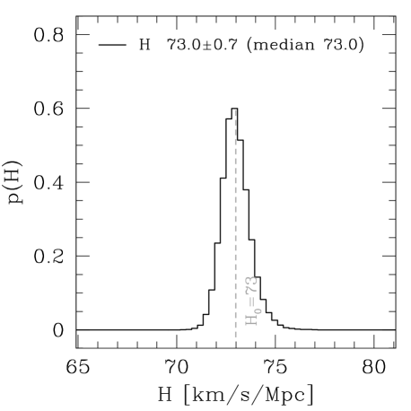
Figure 8: Distribution of Hubble constant values $H$ as measured from the samples containing 12 strong lenses each, are presented (with outlier rejection employed), labeled with the average, dispersion, and median values.

4.4 Simulated measurement of $H_{0}$

Using our data we can simulate the measurement of $H_{0}$ based on a random choice of several of our configurations mimicking small samples of observed lenses with measured time delays. The LOS+ENV approach is the most realistic description of light propagation and we do not show results of other approaches.

We choose from all lenses and all investigated source positions, however we consider only the cases with quadruple images and acceptable fits. When constructing small lens samples we choose a dozen different lenses from a total of 1920 used in simulations. The probability of a lens to be included in a sample is proportional to the surface area of its caustic, which partially reproduces the probability of a lens to produce multiple images. For a given lens we choose at random one from quad image configurations giving satisfactory fits.

For $N$ chosen configurations which give fitted Hubble constant values $H^{i}$ we get the sample average $H$, sample estimated uncertainty $\sigma$, and the estimated error of the average $\Delta H$:

$$H=\frac{1}{N}~{}\sum_{i=1}^{N}~{}H^{i}~{}~{}~{}~{}~{}~{}\sigma^{2}=\frac{\sum~{}(H-H^{i})^{2}}{N-1}~{}~{}~{}~{}~{}~{}\Delta H=\sqrt{\frac{\sigma^{2}}{N}}.$$ (28)

Figure 9: Distributions of estimated errors $\Delta H$ of Hubble constant measurement based on samples of 12 strong lenses with outliers rejection are presented.

We draw a large number of samples of twelve quad lenses each and check the results of $H_{0}$ estimates. Note, that the distribution of fitted values of Hubble constant ($H^{fit}$), as presented on the Fig. 6, has wide wings. The statistics used to form Eq. 28 stems from the considerations with assumed normal distribution of measurement errors. Hence, the measurements coming from the wings of the distribution look like outliers and influence the results considerably. In order to better simulate the real experiment (of measurement of $H_{0}$ from a small sample of real observed gravitational lenses), we introduce an outlier-rejection procedure. For a sample of 12 fiducial measurements, we choose the one that is furthest from the mean in the measures of its uncertainty. Then, we recalculate the mean and uncertainty of the remaining measurements. With such rescaled uncertainties, we test if the initially chosen measurement is further than 3 of its uncertainties from the mean (a $3\sigma$ outlier). If so, we remove it from the sample and repeat the process until no further outliers are found. In 52% of random draws (of 12 measurements) no outliers are found, in 33% one measurement is rejected, in 11% two, and in 3% of draws three measurements are rejected as outliers. We calculate the mean ($H$) of the remaining measurements using Eq. 28. We show the distributions of calculated $H$ in Fig. 8, and of $\Delta H$ in Fig. 9.

The calculation shows that 68% of $H$ values lie within $\pm 0.7~{}\mathrm{km/s/Mpc}$ of $H_{0}$ Thus a twelve lens sample with measured time delays should give consistent estimate of the Hubble constant with $\sim$ 1% relative accuracy (“one sigma”). (Of course only the effects of matter outside the main lens are considered here. The strong lens model is assumed to have a NSIE profile.)

4.5 Strong lenses along LOS

The weak lensing due to LOS perturbs image configurations. Even a weak perturbation, when acting on a configuration with source close to a caustic, may change the number of images or change image properties to an extend preventing their successful modeling. The strong perturbation may give such effects in any case.

We check the effect in the following way. Any of the weak lensing maps from a given atlas is used many times in different combinations with maps from other layers. Using weak lensing maps from one atlas we investigate LOS effects for 160 strong lenses and many source positions. If for an isolated lens (or a lens with neighbours) and some given source position there exists a quad configuration giving a successful simplified fit, we check the existence of quad configurations and their fits, when perturbations by LOS are applied. We list all weak maps involved in failures to get a quad configuration and/or in failures to get a successful fit for cases where quads exist. Then we look for maps, which are overrepresented among those taking part in failures. In each layer we find a map, which is most frequently involved in changing the number of images or in preventing successful fits. We list cases, where the same map in a given layer is most responsible for both kinds of failures. In each of 12 atlases used in calculations there are 2 – 4 such maps and they take part in failures $\sim 3$ times more frequently then average. We then visually examine the suspected maps, usually finding that the deflection and time delay patterns are affected by a strong lens close to the line of sight.

5 Discussion and conclusions

In this paper we have followed the methods of Papers I and II in simulating multiple image configurations of strong gravitational lenses based on the results of Millennium Simulation (Springel et al. 2005, Lemson & Springel 2006). As compared to our previous papers we have changed the method of main lenses selection. We now look for strong haloes in randomly chosen sub regions of Millennium Simulation volume instead of looking for strong lenses inside a simulated wide, low resolution beam of rays. When finding an appropriate candidate we map the matter distribution in its vicinity obtaining a model of strong lens with its environment. When looking for lenses we do not place any extra requirements on their possible environments. (Thus we may be missing some important property of the observed lenses - compare Williams et al., 2006).

We use the mass density profile of the lens from NSIE model and treat it as fixed in our calculations. The parameters of the lens may vary but it remains an isothermal ellipsoid. This guarantees the analytical formulae for the deflection angle and gravitational time delay in our models, but also removes the important source of the uncertainty, the lens mass profile slope degeneracy (compare Suyu, 2012). Thus our estimates of the accuracy of the Hubble constant measurements do not include the uncertainty of the mass profile slope. We do not include external convergence as a parameter in our models.

We have improved our description of matter along the line of sight investigating a large number of cases. In the multiplane approach we use different combinations of weak deflection maps between the observer and the strong lens and between the lens and the source for the fixed strong lensing map and the source position. Thus the influence of different lines of sight on a given source–lens–observer configuration can be examined statistically based on ray tracing. We do not attempt to obtain or employ the relations between the shear, convergence and galaxy over-density near the lens as Suyu et al. (2013), Suyu et al. (2010) do for individual lenses.

Comparison of the typical shear and convergence values used in our simulations (Fig. 1, Fig. 3) with the values employed in modeling of real quad lenses (Wong et al., 2011, Suyu et al., 2010, Suyu et al. (2013)) suggests that our results may have no direct application to the extreme cases analyzed there. According to our study the shear and convergence along random lines of sight are rather small. On the other hand higher than average density of matter along any line of sight makes strong lensing more likely to be observed and may serve as a selection effect not included in our study.

According to our simulations the effects of matter along the line of sight and in the strong lens vicinity are on average weak and do not produce a substantial bias in the expected value of the Hubble constant, which remains close to the true value within $\sim 0.5~{}\mathrm{km/s/Mpc}$. The uncertainty of a measurements based on a single lens is $\sigma\approx 3~{}\mathrm{km/s/Mpc}$, LOS and ENV contributing roughly $2~{}\mathrm{km/s/Mpc}$ each. The distribution is not Gaussian and a probability obtaining a value with $>3~{}\sigma$ error from a single lens is $\sim 3$ per cent. Using a sample of dozen lenses gives the average with $\sim 0.7~{}\mathrm{km/s/Mpc}$ uncertainty.

The external shear can be found by fitting a model to the image configuration or by estimating it from the simulation of light propagation (Eq. 21). Since both methods produce similar results (Fig. 3), we make a numerical experiment substituting the estimated values as model parameters. We also supplement our model with the estimated value of the convergence. As a result we get the new distributions of fitted Hubble constant, which are much more symmetric and narrower as compared to the approach not restricting model parameters. The average values and medians of the $H^{\mathrm{fit}}$ are now at $\leq 0.2~{}\mathrm{km/s/Mpc}$ from the true value and the uncertainty $\sim 2~{}\mathrm{km/s/Mpc}$ - compare Table. 1. This suggests that on average the uncertainty of the Hubble constant measurement resulting from the unknow shear and convergence values is $\sim 2~{}\mathrm{km/s/Mpc}$. It also shows that estimates of the shear and convergence values independent of lens modeling may substantially improve the accuracy of $H_{0}$ measurements, a fact well known to the strong lensing community.

Results of Sec. 3 give a quantitative estimate of the LOS and ENV effects on the time delay distance measurements. We find that using a pair of images and assuming the lens model to be fixed we get $\sim 0.07$ 1-$\sigma$ relative error in the results (Fig. 2). Distances based on fits to the image configurations and derived Hubble constant values (Fig. 6) have the accuracy of $\sim 4$ per cent. Thus our time delay distance estimates remain tentative.

We have simulated a measurement of the Hubble constant based on a small sample of observed time delay lenses drawing the objects from our huge set of fitted lens models. Each sample includes image configurations belonging to different lenses. Drawing the samples large number of times and using a method of outliers elimination, we get distributions of sample-averaged Hubble constant measurements (Figs. 8,  9). Our experiment shows that in 68% of cases the result lies within $\sim 0.7~{}\mathrm{km/s/Mpc}$ or $\sim 1$% from the true (used in the light propagation simulations) value, which should be treated as a line of sight and lens environment only contribution to the error in $H_{0}$.

References

- Ade et al. (2014) Ade, P. A. R. et al. 2014, A&A, 571, A16
- Auger et al. (2007) Auger, M.W., Fassnacht, C.D., Abrahamse, A.L., Lubin, L.M., and Squires, G.K., 2007, AJ, 134, 668
- Bar-Kana (1996) Bar-Kana R., 1996, ApJ, 468, 17
- Bertone et al. (2007) Bertone S., De Lucia G., Thomas P.A., 2007, MNRAS, 379, 1143
- Carbone et al. (2008) Carbone, C., Springel, V., Baccigalupi, C., Bartelmann, M., Matarrese, S., 2008, MNRAS, 388, 1618
- Chen et al. (2003) Chen J., Kravtsov A.V., Keeton C.R., 2003, ApJ, 592, 24
- Collett et al. (2013) Collett, T.E. et al., 2013, MNRAS, 432, 679
- D’Aloisio & Natarajan (2011) D’Aloisio A., Natarajan P., 2011, MNRAS, 411, 1628
- D’Aloisio et al. (2013) D’Aloisio A., Natarajan P., Shapiro, P.R., 2014, MNRAS, 445, 3581
- De Lucia & Blaizot (2007) De Lucia G., Blaizot J., 2007, MNRAS, 375, 2
- Fadely et al. (2010) Fadely, R., Keeton, C.R., Nakajima, R., Bernstein, G.M., 2010, ApJ, 711, 246
- Freedman & Madore (2010) Freedman, W.L., Madore, B.F., 2010, ARAA, 48, 673
- Gorenstein et al. (1988) Gorenstein, M.V., Falco, E.E., Shapiro, I.I., 1988, ApJ, 327, 693
- Hinshaw et al. (2013) Hinshaw, G. et al., 2013, ApJS, 208, 19
- Hilbert et al. (2007) Hilbert, S., White, S.D., Hartlap, J., Schneider, P.,2007, MNRAS, 382, 121
- Hilbert et al. (2009) Hilbert, S., White, S.D., Hartlap, J., Schneider, P.,2009, A&A, 499, 31
- (17) Jaroszynski M., Kostrzewa-Rutkowska Z., 2012, MNRAS, 424, 325 (Paper I)
- (18) Jaroszynski M., Kostrzewa-Rutkowska Z., 2014, MNRAS, 439, 2432 (Paper II)
- Jee et al. (2015) Jee, I., Komatsu, E., Suyu, S.H., 2015, JCAP, 11, 033
- Keeton et al. (1997) Keeton C. R., Kochanek C. S., Seljak U., 1997, ApJ, 487, 42
- Keeton & Zabludoff (2004) Keeton C. R., Zabludoff, A.I., 2004, ApJ, 612, 660
- Kimm & Yi (2007) MKimm T., Yi S.K., 2007, ApJ, 670, 1048
- Kochanek (2006) Kochanek C.S., 2006, in: Gravitational Lensing: Strong, Weak and Micro, Saas-Fee Advanced Course 33, Springer, Berlin
- Kochanek & Apostolakis (1988) Kochanek C.S., Apostolakis J., 1988, MNRAS, 235, 1073
- Kormann et al. (1994) Kormann R., Schneider P., Bartelmann M., 1994, A&A, 284, 285
- Lemson & Springel (2006) Lemson G. , Springel V., 2006, Astr.Soc.Pac.Conf., 351, 212
- McCully et al. (2014) McCully, C., Keeton C., Wong, K.C., Zabludoff A.,2014, MNRAS, 443, 3631
- McCully et al. (2016) McCully, C., Keeton C., Wong, K.C., Zabludoff A.,2016, arXiv:1601.05417
- Momcheva et al. (2006) Momcheva, I., Williams K., Keeton C., Zabludoff A.,2006, 641, 169
- Oguri (2007) Oguri, M.,2007, ApJ, 660, 1
- Paraficz & Hjorth (2009) Paraficz, D., Hjorth, J., 2009, A&A, 507, L49
- Paraficz & Hjorth (2010) Paraficz, D., Hjorth, J., 2010, ApJ, 712, 1378
- Rathna Kumar et al. (2015) Rathna Kumar, S., Stalin, C.S., Prabhu, T.P., 2015, A&A, 580, A38
- Refsdal (1964) Refsdal, S., 1964, MNRAS, 128, 307
- Riess et al. (2011) Riess, A.G., 2011, ApJ, 730, 119
- Schneider et al. (1992) Schneider P., Ehlers J., Falco E.E., 1992, “Gravitational Lenses”, Springer-Verlag Berlin Heidelberg New York
- Schneider & Weiss (1988) Schneider P., Weiss A., 1988, ApJ, 327, 526
- Springel et al. (2005) Springel V., White S.D.M., Jenkins A., et al., 2005, Nature, 435, 629
- Seitz & Schneider (1992) Seitz S. Schneider P., 1992, A&A, 265, 1
- Schneider (2014a) Schneider P., 2014, A&A, 568, L2
- Schneider (2014b) Schneider P., 2014, arXiv:1409.0015
- Smith et al. (2014) Smith, M., et al., 2014, Apj, 780, 24
- Suyu (2012) Suyu S.H., 2012, MNRAS, 426, 868
- Suyu et al. (2013) Suyu S.H., Auger M.W., Hilbert, S. et al., 2013, ApJ, 766, 70
- Suyu et al. (2010) Suyu S.H., Marshall P.J., Auger M.W., Hilbert, S., Blandford R.D., Koopmans L.V.E., Fassnacht C.D., Treu T., 2010, Apj, 711, 201
- Wambsganss et al. (2004) Wambsganss J., Bode P., Ostriker J.P., 2004, ApJ, 606, L93
- Wambsganss et al. (2005) Wambsganss J., Bode P., Ostriker J.P., 2005, ApJ, 635, L1
- Williams et al. (2006) Williams K.A., Momcheva I., Keeton C.R., Zabludoff A.I., Lehar J., 2006, ApJ, 646, 85
- Wong et al. (2011) Wong, K.C., Keeton C.R., Williams K.A., Momcheva I.G., Zabludoff A.I., 2011, ApJ, 726, 84