Radiative transfer of acoustic waves in continuous complex media: Beyond the Helmholtz equation

Abstract

Heterogeneity can be accounted for by a random potential in the wave equation. For acoustic waves in a fluid with fluctuations of both density and compressibility (as well as for electromagnetic waves in a medium with fluctuation of both permittivity and permeability) the random potential entails a scalar and an operator contribution. For simplicity, the latter is usually overlooked in multiple scattering theory: whatever the type of waves, this simplification amounts to considering the Helmholtz equation with a sound speed $c$ depending on position $\boldsymbol{\mathbf{r}}$. In this work, a radiative transfer equation is derived from the wave equation, in order to study energy transport through a multiple scattering medium. In particular, the influence of the operator term on various transport parameters is studied, based on the diagrammatic approach of multiple scattering. Analytical results are obtained for fundamental quantities of transport theory such as the transport mean-free path $\ell^{*}$, scattering phase function $f$ and anisotropy factor $g$. Discarding the operator term in the wave equation is shown to have a significant impact on $f$ and $g$, yet limited to the low-frequency regime i.e., when the correlation length of the disorder $\ell_{c}$ is smaller than or comparable to the wavelength $\lambda$. More surprisingly, discarding the operator part has a significant impact on the transport mean-free path $\ell^{*}$ whatever the frequency regime. When the scalar and operator terms have identical amplitudes, the discrepancy on the transport mean-free path is around $300\%$ in the low-frequency regime, and still above $30\%$ for $\ell_{c}/\lambda=10^{3}$ no matter how weak fluctuations of the disorder are. Analytical results are supported by numerical simulations of the wave equation and Monte Carlo simulations.

I Introduction

Understanding the propagation of classical waves through strongly scattering media is of great importance for many applications such as imaging, characterization or communication with all kinds of waves Sebbah (2001); van Tiggelen and Skipetrov (2003); Sato et al. (2012); Mosk et al. (2012).

When dealing with wave propagation a first step consists in considering an inhomogeneous medium as one particular realization of a random process. Instead of calculating the wave field exactly for one configuration, one considers statistical averages of the wavefield and of its intensity. They can be determined by solving two fundamental equations: Dyson’s equation for the coherent field (i.e., the ensemble-averaged wavefield) and the Bethe-Salpether equation for the correlation of the wavefield. Both can be derived from the wave equation, within the diagrammatic approach of multiple scattering Foldy (1945); Frisch (1968); Kravtsov et al. (1989); Barabanenkov (1968); Sheng (2006); Akkermans and Montambaux (2007); van Rossum and Nieuwenhuizen (1999).

Once Dyson’s equation is solved, the effective phase and group velocities as well as the scattering mean-free path $\ell_{s}$ can be determined. From a physical point of view, as the wave propagates over a distance $z$, the intensity of the coherent part decays exponentially as $\exp(-z/\ell_{s})$ to the benefit of the incoherent contribution. In order to calculate the total intensity (both coherent and incoherent) it is necessary to solve the Bethe-Salpether equation. It has been long established that the Bethe-Salpether equation can be simplified into a transport equation termed the radiative transfer equation (RTE). Further approximations lead to an even simpler equation, the diffusion equation, which has analytical solutions and is essentially characterized by one parameter: the diffusion constant or diffusivity $D=\ell^{*}c_{\text{tr}}/3$, with $\ell^{*}$ the transport mean-free path and $c_{\text{tr}}$ the transport speed.

In acoustics, heterogeneity originates from space-dependence of mass density and elastic constants. From an experimental point of view, a ballistic to diffuse transition occurs as the thickness of the sample increases. Transport parameters ($\ell_{s}$, $D$, $\ell^{*}$, $c_{\text{tr}}$) can be estimated from experimental measurements, for instance by studying the average transmitted flux as a function of time Zhang et al. (1999); Page et al. (1995); Ramamoorthy et al. (2004); Weaver and Sachse (1995); Weaver (1990); Page et al. (1997). A key question is: to what extent does an estimation of the transport parameters lead to a reliable information about structural properties of the medium (correlation lengths, variance of mass density and elastic constants)?

In the present paper, we are interested in constructing a complete radiative transfer model for acoustic waves propagating in a continuous but heterogeneous fluid. We focus on one particular aspect: unlike Helmholtz’ equation, where heterogeneity only appears in a space-dependence of the sound speed, the full wave equation is taken into account. It includes a random operator term which complicates the analysis, as will be detailed later. Discarding it, as is usually done, amounts to considering as a starting point the Helmholtz equation, with a space-dependent sound speed $c(\boldsymbol{\mathbf{r}})$ as the only source of disorder. The question we address here is the impact of the operator term in the wave equation on the final result, i.e. the parameters that appear in the RTE and finally in the diffusion equation. When studying energy transmission in a continuous multiple scattering medium, under which conditions is it justified to discard the operator term in the wave equation?

Note that radiative transfer equations can be phenomenologically established without further reference to the underlying wave equation or medium characteristics. This is why a complete derivation of the RTE starting from the correct wave equation is necessary here, in order to relate the transport parameters to the microstuctural properties (correlation lengths and variances) of the heterogeneities, which is the core of the paper. Here, we deal with acoustic waves but the exact same questions arise for transport of electromagnetic energy in a medium with fluctuations of both permeability and permittivity, and can be addressed with the same tools Tsang and Kong (2001).

From a theoretical point of view, in a continuous heterogeneous fluid without dissipation, the starting point is the following wave equation Chernov (1960); Ross and Chivers (1986) for the acoustic pressure $p\left(\boldsymbol{\mathbf{r}},t\right)$:

$$\Delta p-\frac{1}{c_{0}^{2}}\frac{\partial^{2}p}{\partial t^{2}}=\boldsymbol{\mathbf{\nabla}}\beta\left(\boldsymbol{\mathbf{r}}\right)\cdot\boldsymbol{\mathbf{\nabla}}p-\frac{\alpha\left(\boldsymbol{\mathbf{r}}\right)}{c_{0}^{2}}\frac{\partial^{2}p}{\partial t^{2}}$$ (1)

where $c_{0}$ is a reference sound speed. Note that throughout the paper, the symbols used for the wave fields (pressure $p\left(\boldsymbol{\mathbf{r}},t\right)$, velocity $\boldsymbol{\mathbf{v}}\left(\boldsymbol{\mathbf{r}},t\right)$) actually refer to the complex-valued analytic signals associated to the real quantities. In Eq. (1), heterogeneity arises from spatial fluctuations of two dimensionless functions of space $\alpha$ and $\beta$ which are related to mass density $\rho(\boldsymbol{\mathbf{r}})$ and compressibility $\chi(\boldsymbol{\mathbf{r}})$ by

$$\alpha\left(\boldsymbol{\mathbf{r}}\right) =1-\left[\frac{c_{0}}{c\left(\boldsymbol{\mathbf{r}}\right)}\right]^{2},$$ (2)

$$\beta\left(\boldsymbol{\mathbf{r}}\right) =\ln\left[\frac{\rho\left(\boldsymbol{\mathbf{r}}\right)}{\rho_{0}}\right]$$ (3)

where the space-dependent sound speed is $c(\boldsymbol{\mathbf{r}})=1/\sqrt{\rho(\boldsymbol{\mathbf{r}})\chi(\boldsymbol{\mathbf{r}})}$. $\rho_{0}$ is an arbitrary constant with the dimension of a mass density. In the frequency domain (angular frequency $\omega$), the Fourier transform of Eq. (1) for the acoustic pressure $P\left(\boldsymbol{\mathbf{r}},\omega\right)$ becomes

$$\Delta P+k_{0}^{2}P=k_{0}^{2}\gamma P.$$ (4)

$k_{0}=\omega/c_{0}$ and $\gamma$ is a random potential that entails both a scalar and operator term in the form

$$\gamma\left(\boldsymbol{\mathbf{r}}\right)=\alpha\left(\boldsymbol{\mathbf{r}}\right)+\frac{1}{k_{0}^{2}}\boldsymbol{\mathbf{\nabla}}\beta\left(\boldsymbol{\mathbf{r}}\right)\cdot\boldsymbol{\mathbf{\nabla}}.$$ (5)

Provided the statistical properties of $\alpha$ and $\beta$, particularly their correlation functions, are known, the ensemble-averaged (or coherent) field $\left\langle P\right\rangle$ can be calculated, as well as the autocorrelation $\left\langle PP^{*}\right\rangle$.

It is usual to discard the operator term in Eq. (5), which greatly simplifies the calculations. This relies on the assumption that $c(\boldsymbol{\mathbf{r}})$ alone fully describes the heterogeneity of the medium, and in the following it will be referred to as the scalar approximation. It is true if the mass density is constant in space. It is also true if the mass density is not constant, as long as the compressibility is: in that case, the acoustic wave equation for the velocity potential only involves $\alpha$ and not $\gamma$. However, when fluctuations of mass density and compressibility coexist and have comparable amplitudes, no matter how weak they are, it results in an important error in the scattering mean-free path $\ell_{s}$ at low frequency i.e., when the correlation length is comparable to or smaller than the wavelength Baydoun et al. (2015). In that case one has to use the complete expression for the potential $\gamma$ defined in Eq. (5). The self-energy $\Sigma$, which is the key quantity for evaluating the average field through the Dyson equation, can be determined using the diagrammatic approach of multiple scattering. $\Sigma$ contains three additional terms due to the operator part in Eq. (5), which are not taken into account under the scalar approximation Jones (1999); Baydoun et al. (2015); Zhuck (1995).

Beyond the self-energy $\Sigma$, here we are interested in the intensity operator $K$ which is the key quantity in the Bethe-Salpeter equation, thus driving the average intensity and correlation function of the wavefield. Particularly we aim at evaluating the impact of the scalar approximation on $K$ and consequently on the transport parameters.

The rest of the paper is organised as follows. Sections II and III give an overview of the quantities and parameters that are essential to account for energy transport in random media, and how they are related to the random potential $\gamma$ in the wave equation. In Section IV, analytical solutions are calculated in the case of an exponentially-correlated disorder. They yield expressions for the transport parameters, with or without the operator term. In order to validate the analytical results, numerical simulations of the wave equation are performed on an ensemble of realizations. The average transmitted energy flux is calculated as a function of time, and compared to the solution of the RTE with the transport parameters derived analytically. In that case the RTE is solved numerically with a Monte Carlo approach. Section V concludes the paper.

II An overview of radiative transfer

Let us first consider the case of a homogeneous and lossless medium (reference medium). In a monochromatic regime, the free-space Green function $G_{0}\left(\boldsymbol{\mathbf{r}},\boldsymbol{\mathbf{r}}_{s}\right)$ is the solution of the wave equation for a point source located at $\boldsymbol{\mathbf{r}}_{s}$:

$$\Delta G_{0}+k_{0}^{2}G_{0}=\delta\left(\boldsymbol{\mathbf{r}}-\boldsymbol{\mathbf{r}}_{s}\right).$$ (6)

The causal solution of Eq. (6) is $G_{0}(\boldsymbol{\mathbf{r}}-\boldsymbol{\mathbf{r}}_{s})=-\exp[jk_{0}|\boldsymbol{\mathbf{r}}-\boldsymbol{\mathbf{r}}_{s}|]/[4\pi|\boldsymbol{\mathbf{r}}-\boldsymbol{\mathbf{r}}_{s}|]$. For a heterogeneous fluid, the Green function $G\left(\boldsymbol{\mathbf{r}},\boldsymbol{\mathbf{r}}_{s}\right)$ associated to Eq. (4) satisfies:

$$\Delta G+k_{0}^{2}G=k_{0}^{2}\gamma G+\delta\left(\boldsymbol{\mathbf{r}}-\boldsymbol{\mathbf{r}}_{s}\right).$$ (7)

Note that the dependency of $G$ and $G_{0}$ on $\omega$ will only be made explicit (via the function’s argument) when different frequencies are involved. In the presence of an arbitrary distribution of sources $S(\boldsymbol{\mathbf{r}}_{s})$ in the right-hand side of Eq. (4), the resulting field is

$$P\left(\boldsymbol{\mathbf{r}},\omega\right)=\int G\left(\boldsymbol{\mathbf{r}},\boldsymbol{\mathbf{r}}_{s}\right)S\left(\boldsymbol{\mathbf{r}}_{s}\right)\mathrm{d}\boldsymbol{\mathbf{r}}_{s}.$$ (8)

The perturbed Green’s function $G\left(\boldsymbol{\mathbf{r}},\boldsymbol{\mathbf{r}}_{s}\right)$ can be understood as the solution of Eq. (6) with an additional source term equal to $k_{0}^{2}\gamma G$, involving $G$ itself. Hence, it is usual to express it in a recursive (Lippman-Schwinger) form:

$$G\left(\boldsymbol{\mathbf{r}},\boldsymbol{\mathbf{r}}_{s},\omega\right)=G_{0}\left(\boldsymbol{\mathbf{r}},\boldsymbol{\mathbf{r}}_{s},\omega\right)\\ +k_{0}^{2}\int G_{0}\left(\boldsymbol{\mathbf{r}},\boldsymbol{\mathbf{r}}_{1},\omega\right)V\left(\boldsymbol{\mathbf{r}}_{1},\boldsymbol{\mathbf{r}}_{2}\right)G\left(\boldsymbol{\mathbf{r}}_{2},\boldsymbol{\mathbf{r}}_{s},\omega\right)\mathrm{d}\boldsymbol{\mathbf{r}}_{1}\mathrm{d}\boldsymbol{\mathbf{r}}_{2},$$ (9)

where a two-variable random potential $V\left(\boldsymbol{\mathbf{r}}_{1},\boldsymbol{\mathbf{r}}_{2}\right)$ is defined in terms of $\gamma$ as follows:

$$V\left(\boldsymbol{\mathbf{r}}_{1},\boldsymbol{\mathbf{r}}_{2}\right)=\gamma\left(\boldsymbol{\mathbf{r}}_{1}\right)\delta\left(\boldsymbol{\mathbf{r}}_{1}-\boldsymbol{\mathbf{r}}_{2}\right)=\alpha\left(\boldsymbol{\mathbf{r}}_{1}\right)\delta\left(\boldsymbol{\mathbf{r}}_{1}-\boldsymbol{\mathbf{r}}_{2}\right)\\ +\frac{1}{k_{0}^{2}}\boldsymbol{\mathbf{\nabla}}\beta\left(\boldsymbol{\mathbf{r}}_{1}\right)\cdot\boldsymbol{\mathbf{\nabla}}\delta\left(\boldsymbol{\mathbf{r}}_{1}-\boldsymbol{\mathbf{r}}_{2}\right).$$ (10)

II.1 Average field: Dyson’s equation

Considering $\alpha$ and $\beta$ as random variables with known statistical parameters, we are now interested in determining the ensemble average of the Green function, $\langle G\rangle$. Iteratively substituting $G$ under the integral on the right hand side of Eq. (9) provides an infinite sum of integrals known as Born’s expansion. After ensemble averaging this expansion, it can be shown that $\langle G\rangle$ obeys Dyson’s equation Kravtsov et al. (1989):

$$\left\langle G\left(\boldsymbol{\mathbf{r}},\boldsymbol{\mathbf{r}}_{s}\right)\right\rangle=G_{0}\left(\boldsymbol{\mathbf{r}},\boldsymbol{\mathbf{r}}_{s}\right)\\ +k_{0}^{2}\int G_{0}\left(\boldsymbol{\mathbf{r}},\boldsymbol{\mathbf{r}}_{1}\right)\Sigma\left(\boldsymbol{\mathbf{r}}_{1},\boldsymbol{\mathbf{r}}_{2}\right)\left\langle G\left(\boldsymbol{\mathbf{r}}_{2},\boldsymbol{\mathbf{r}}_{s}\right)\right\rangle\mathrm{d}\boldsymbol{\mathbf{r}}_{1}\mathrm{d}\boldsymbol{\mathbf{r}}_{2}.$$ (11)

$\Sigma$ is the self-energy or mass operator and accounts for all orders of multiple scattering events which cannot be factorized in the ensemble average process. Assuming that the medium is statistically homogeneous, $V$, $G_{0}$ and consequently $\Sigma$ and $\left\langle G\right\rangle$ are invariant under translation. In that case Eq. (11) is a double convolution product. Therefore, its spatial Fourier transform, denoted by a tilde $\widetilde{\cdot}$ symbol, is

$$\left\langle\widetilde{G}\left(\boldsymbol{\mathbf{k}}\right)\right\rangle=\frac{1}{k_{0}^{2}-k^{2}-\widetilde{\Sigma}\left(\boldsymbol{\mathbf{k}},\omega\right)},$$ (12)

where $\boldsymbol{\mathbf{k}}$ is the dual variable for $\boldsymbol{\mathbf{r}}-\boldsymbol{\mathbf{r}}_{s}$.

Performing an inverse Fourier transform and taking into account the source distribution yields the coherent field

$$\left\langle P\left(\boldsymbol{\mathbf{r}},\omega\right)\right\rangle=\int\left\langle G\left(\boldsymbol{\mathbf{r}}-\boldsymbol{\mathbf{r}}_{s}\right)\right\rangle S\left(\boldsymbol{\mathbf{r}}_{s}\right)\mathrm{d}\boldsymbol{\mathbf{r}}_{s}.$$ (13)

The last step in determining $\left\langle G\right\rangle$ would be to obtain an explicit expression of $\Sigma$. Unfortunately, the exact calculation is intractable in most cases of interest. But an expression as a series of Feynman’s diagrams can be derived and has been extensively discussed in Refs Frisch, 1968 and Kravtsov et al., 1989. The second-order approximation of this series, known as the Bourret approximation, will be used in section III to derive an expression of $\Sigma$ valid for weakly disordered systems ($k_{0}\ell_{s}\gg 1$). A complete analysis of the coherent field’s propagation is not our present purpose and the interested reader may refer to Ref. Baydoun et al., 2015 for details. Importantly, the intensity of the coherent field, also known as the coherent or ballistic intensity, is shown to be spatially damped with a decay length $\ell_{s}$. When $\alpha$ and $\beta$ have similar fluctuations, the scalar approximation has been shown to significantly overestimate $\ell_{s}$ at low frequencies, but is reasonably valid as long as $k_{0}\ell_{c}>10$ Baydoun et al. (2015) where $\ell_{c}$ is the correlation length of the disorder.

II.2 Two-point correlation of the field: Bethe-Salpeter equation

The intensity of the average field only describes coherent transmission through a disordered medium, it does not suffice to account for total energy transmission, both coherent and incoherent. To do so, since all physical quantities related to average energy involve average products of two wavefields, the essential ingredient is the two-point correlation function $\left\langle P\left(\boldsymbol{\mathbf{r}},\omega^{+}\right)P^{*}\left(\boldsymbol{\mathbf{r}}^{\prime},\omega^{-}\right)\right\rangle$ where $\cdot^{*}$ indicates a complex conjugation and $\omega^{\pm}$ denote angular frequencies. It is known to obey the Bethe-Salpeter equation Frisch (1968); Kravtsov et al. (1989); Anisovich et al. (1993) which reads

$$\left\langle P\left(\boldsymbol{\mathbf{r}},\omega^{+}\right)P^{*}\left(\boldsymbol{\mathbf{r}}^{\prime},\omega^{-}\right)\right\rangle=\left\langle P\left(\boldsymbol{\mathbf{r}},\omega^{+}\right)\right\rangle\left\langle P^{*}\left(\boldsymbol{\mathbf{r}}^{\prime},\omega^{-}\right)\right\rangle\\ +\int\mathrm{d}\boldsymbol{\mathbf{r}}_{1}\mathrm{d}\boldsymbol{\mathbf{r}}_{2}\mathrm{d}\boldsymbol{\mathbf{\uprho}}_{1}\mathrm{d}\boldsymbol{\mathbf{\uprho}}_{2}\left\langle G\left(\boldsymbol{\mathbf{r}},\boldsymbol{\mathbf{r}}_{1},\omega^{+}\right)\right\rangle\left\langle G^{*}\left(\boldsymbol{\mathbf{r}}^{\prime},\boldsymbol{\mathbf{r}}_{2},\omega^{-}\right)\right\rangle\\ \times K\left(\boldsymbol{\mathbf{r}}_{1},\boldsymbol{\mathbf{r}}_{2},\boldsymbol{\mathbf{\uprho}}_{1},\boldsymbol{\mathbf{\uprho}}_{2},\omega^{+},\omega^{-}\right)\left\langle P\left(\boldsymbol{\mathbf{\uprho}}_{1},\omega^{+}\right)P^{*}\left(\boldsymbol{\mathbf{\uprho}}_{2},\omega^{-}\right)\right\rangle.$$ (14)

$K$ is termed the intensity operator (or “irreducible vertex”). Similarly to the self-energy $\Sigma$ for the average field, $K$ can be expressed as a perturbative expansion taking into account all orders of multiple scattering events. It is in general represented by Feynman diagrams for convenience. In section III, the first order expansion, valid for weakly disordered systems and known as the Ladder approximation, will be used. Dropping the $\omega^{\pm}$ dependency for brevity, the spatial Fourier transform of $K$ is defined by

$$\widetilde{K}\left(\boldsymbol{\mathbf{k}}_{1},\boldsymbol{\mathbf{k}}_{2},\boldsymbol{\mathbf{q}}_{1},\boldsymbol{\mathbf{q}}_{2}\right)=\int\mathrm{d}\boldsymbol{\mathbf{r}}_{1}\mathrm{d}\boldsymbol{\mathbf{r}}_{2}\mathrm{d}\boldsymbol{\mathbf{\uprho}}_{1}\mathrm{d}\boldsymbol{\mathbf{\uprho}}_{2}K\left(\boldsymbol{\mathbf{r}}_{1},\boldsymbol{\mathbf{r}}_{2},\boldsymbol{\mathbf{\uprho}}_{1},\boldsymbol{\mathbf{\uprho}}_{2}\right)\\ \times\exp\left[j\left(-\boldsymbol{\mathbf{r}}_{1}\cdot\boldsymbol{\mathbf{k}}_{1}+\boldsymbol{\mathbf{r}}_{2}\cdot\boldsymbol{\mathbf{k}}_{2}+\boldsymbol{\mathbf{\uprho}}_{1}\cdot\boldsymbol{\mathbf{q}}_{1}-\boldsymbol{\mathbf{\uprho}}_{2}\cdot\boldsymbol{\mathbf{q}}_{2}\right)\right].$$ (15)

Assuming that the medium is stastistically homogeneous, ${K}$ is invariant under spatial translation which implies in the Fourier space

$$\widetilde{K}\left(\boldsymbol{\mathbf{k}}_{1},\boldsymbol{\mathbf{k}}_{2},\boldsymbol{\mathbf{q}}_{1},\boldsymbol{\mathbf{q}}_{2}\right)=\\ \left(2\pi\right)^{3}\delta\left(\boldsymbol{\mathbf{k}}_{1}-\boldsymbol{\mathbf{k}}_{2}-\boldsymbol{\mathbf{q}}_{1}+\boldsymbol{\mathbf{q}}_{2}\right)\widetilde{\varGamma}\left(\boldsymbol{\mathbf{k}}_{1},\boldsymbol{\mathbf{k}}_{2},\boldsymbol{\mathbf{q}}_{1},\boldsymbol{\mathbf{q}}_{2}\right).$$ (16)

II.3 Radiative transfer equation

In many configurations of interest, the average envelope of the wavefield $\left\langle\left|p(\boldsymbol{\mathbf{r}},t)\right|\right\rangle$ varies at a time scale much larger than the oscillations of the field, and its spatial variation occur at a characteristic scale much larger than the wavelength. This is sometimes referred to as the separation of scales hypothesis. Under this approximation and for weakly disordered systems, it can be shown (see App. A for details), that Eq. (14) can be transformed into the following transport equation, known as the Radiative Transfer Equation (RTE) Chandrasekhar (1950); Margerin (2005); Turner and Weaver (1994); Apresyan and Kravtsov (1996)

$$\left[\frac{\partial_{\tau}}{c_{\text{tr}}}+\hat{\boldsymbol{\mathbf{k}}}\cdot\boldsymbol{\mathbf{\nabla}}_{\boldsymbol{\mathbf{r}}}\right]\mathcal{I}\left(\boldsymbol{\mathbf{r}},\hat{\boldsymbol{\mathbf{k}}},\tau,\omega\right)=-\underbrace{\frac{1}{\ell_{e}}\mathcal{I}\left(\boldsymbol{\mathbf{r}},\hat{\boldsymbol{\mathbf{k}}},\tau,\omega\right)}_{\text{loss}}\\ +\underbrace{\frac{1}{4\pi\ell_{s}}\int_{4\pi}\mathrm{d}\Omega_{\hat{\boldsymbol{\mathbf{q}}}}f\left(\hat{\boldsymbol{\mathbf{k}}},\hat{\boldsymbol{\mathbf{q}}},\omega\right)\mathcal{I}\left(\boldsymbol{\mathbf{r}},\hat{\boldsymbol{\mathbf{q}}},\tau,\omega\right)}_{\text{gain}}+\underbrace{\mathcal{S}(\boldsymbol{\mathbf{r}},\hat{\boldsymbol{\mathbf{k}}},\tau,\omega)}_{\text{source}}.$$ (17)

The physical quantity of interest in Eq. (17) is the specific intensity $\mathcal{I}$. Mathematically, it can be rigorously defined as a Wigner transform of the wavefield (see App. A). Physically, $\mathcal{I}$ may be interpreted as the local power density per unit surface at point $\boldsymbol{\mathbf{r}}$ and time $\tau$ flowing in the direction of the unit vector $\hat{\boldsymbol{\mathbf{k}}}$ when a quasi-monochromatic wave (central frequency $\omega/2\pi$) is emitted into a random medium. The left-hand side of Eq. (17) involves a Lagrangian derivative $\mathrm{d}\mathcal{I}/\mathrm{d}\tau$, in the direction $\hat{\boldsymbol{\mathbf{k}}}$ at speed $c_{\text{tr}}$. If the medium was homogeneous the loss and gain terms would vanish, meaning that the amount of energy flowing in any direction $\hat{\boldsymbol{\mathbf{k}}}$ would not change over time unless some energy is provided by the source. Inhomogeneity (hence scattering) appears in the first two terms of the right-hand side. The extinction term $-\mathcal{I}/\ell_{e}$ describes power losses away from direction $\hat{\boldsymbol{\mathbf{k}}}$ due to scattering between $\tau$ and $\tau+\mathrm{d}\tau$. On the contrary, the following term in Eq. (17) describes power gained from all directions $\hat{\boldsymbol{\mathbf{q}}}$ into $\hat{\boldsymbol{\mathbf{k}}}$, due to scattering. The last term is the amount of power per unit volume injected in the medium by the source. As a whole, Eq. (17) describes an energy balance: variation of $\mathcal{I}$ between $\tau$ and $\tau+\mathrm{d}\tau$ is due to loss, gain and source. The RTE has five essentiel ingredients: a particular wavenumber $k_{r}$, a transport speed $c_{\text{tr}}$, an extinction length $\ell_{e}$, a scattering length $\ell_{s}$ and a phase function $f$. The latter represents the probability of sound propagating in direction $\hat{\boldsymbol{\mathbf{q}}}$ to be scattered into the solid angle $\mathrm{d}\Omega_{\hat{\boldsymbol{\mathbf{k}}}}$ around $\boldsymbol{\mathbf{k}}$. In the detailed derivation of the RTE, these parameters are respectively given by (see Apps. B and C)

$$k_{r}^{2}\left(\omega\right) =\operatorname{Re}\left[k_{0}^{2}-\widetilde{\Sigma}\left(k_{r},\omega\right)\right],$$ (18)

$$c_{\text{tr}}\left(\omega\right) =c_{0}^{2}k_{r}\left(\omega\right)/\omega,$$ (19)

$$\frac{1}{\ell_{e}\left(\omega\right)} =-\frac{1}{k_{r}}\operatorname{Im}\left[\widetilde{\Sigma}\left(k_{r},\omega\right)\right],$$ (20)

$$\frac{1}{\ell_{s}\left(\omega\right)} =\frac{1}{16\pi^{2}}\int_{4\pi}\widetilde{\varGamma}\left(k_{r}\hat{\boldsymbol{\mathbf{k}}},k_{r}\hat{\boldsymbol{\mathbf{k}}},k_{r}\hat{\boldsymbol{\mathbf{q}}},k_{r}\hat{\boldsymbol{\mathbf{q}}},\omega,\omega\right)\mathrm{d}\Omega_{\hat{\boldsymbol{\mathbf{q}}}},$$ (21)

$$f\left(\hat{\boldsymbol{\mathbf{k}}}\cdot\hat{\boldsymbol{\mathbf{q}}},\omega\right) =\frac{\ell_{s}(\omega)}{4\pi}\widetilde{\varGamma}\left(k_{r}\hat{\boldsymbol{\mathbf{k}}},k_{r}\hat{\boldsymbol{\mathbf{k}}},k_{r}\hat{\boldsymbol{\mathbf{q}}},k_{r}\hat{\boldsymbol{\mathbf{q}}},\omega,\omega\right).$$ (22)

In these expressions, we have used the fact that the medium is also statistically isotropic. It implies that $\widetilde{\Sigma}(\boldsymbol{\mathbf{k}})$ and $\widetilde{\varGamma}\left(k_{r}\hat{\boldsymbol{\mathbf{k}}},k_{r}\hat{\boldsymbol{\mathbf{k}}},k_{r}\hat{\boldsymbol{\mathbf{q}}},k_{r}\hat{\boldsymbol{\mathbf{q}}}\right)$ depend only on $|\boldsymbol{\mathbf{k}}|$ and $\hat{\boldsymbol{\mathbf{k}}}\cdot\hat{\boldsymbol{\mathbf{q}}}$ respectively [see Eq. (16)]. Equation (18) gives an implicit expression for $k_{r}$, a quantity necessary to determine all other parameters entering the RTE. The last step to fully determine the five coefficients [Eqs. (19) to (22)] consists in relating them to the microscopic features of the heterogeneous medium, particularly the correlation function of the random potential in the wave equation. This is the subject of the next section.

III Expressions of the RTE parameters

III.1 First-order smoothing approximation and its relation to energy conservation

At this point, it is necessary to specify the perturbative development of $\Sigma$ and $K$ as infinite series of scattering diagrams, in order to derive explicit expressions of the extinction ($\ell_{e}$) and scattering ($\ell_{s}$) lengths and of the phase function $f$. With the usual conventions, the development of $\Sigma$ can be represented as

$$\Sigma=\psset{unit=4.26791pt,fillstyle=solid,fillcolor=white}\begin{pspicture}[missing](0.0pt,-12.80374pt)(8.53583pt,12.80374pt){\pscircle(4.26791pt,0.0pt){4.26791pt}}\end{pspicture}+\psset{unit=4.26791pt,fillstyle=solid,fillcolor=white}\begin{pspicture}[missing](0.0pt,-12.80374pt)(34.14331pt,12.80374pt){\psset{linestyle=dashed}\psarc(17.07166pt,0.0pt){12.80374pt}{0.0}{180.0}}{\psline(4.26791pt,0.0pt)(29.8754pt,0.0pt)}{\pscircle(4.26791pt,0.0pt){4.26791pt}}{\pscircle(29.8754pt,0.0pt){4.26791pt}}\end{pspicture}+\psset{unit=4.26791pt,fillstyle=solid,fillcolor=white}\begin{pspicture}[missing](0.0pt,-12.80374pt)(59.7508pt,25.60748pt){\psset{linestyle=dashed}\psarc(29.8754pt,0.0pt){25.60748pt}{0.0}{180.0}}{\psline(4.26791pt,0.0pt)(29.8754pt,0.0pt)}{\psline(29.8754pt,0.0pt)(55.48288pt,0.0pt)}{\pscircle(4.26791pt,0.0pt){4.26791pt}}{\pscircle(29.8754pt,0.0pt){4.26791pt}}{\pscircle(55.48288pt,0.0pt){4.26791pt}}\end{pspicture}+\ldots$$ (23)

In this representation, circles denote scattering events (potential $V$), horizontal solid lines represent free-space Green functions $G_{0}$ and dashed lines stand for spatial correlation between points. Regarding $K$, we have

$$K=\psset{unit=4.26791pt,fillstyle=solid,fillcolor=white}\begin{pspicture}[missing](0.0pt,-25.60748pt)(8.53583pt,25.60748pt){\psset{linestyle=dashed}\psline(4.26791pt,12.80374pt)(4.26791pt,-12.80374pt)}{\pscircle(4.26791pt,-12.80374pt){4.26791pt}}{\pscircle(4.26791pt,12.80374pt){4.26791pt}}\end{pspicture}+\psset{unit=4.26791pt,fillstyle=solid,fillcolor=white}\begin{pspicture}[missing](0.0pt,-25.60748pt)(34.14331pt,25.60748pt){\psset{linestyle=dashed}\psarc(17.07166pt,12.80374pt){12.80374pt}{0.0}{180.0}}{\psset{linestyle=dashed}\psline(4.26791pt,12.80374pt)(4.26791pt,-12.80374pt)}{\psline(4.26791pt,12.80374pt)(29.8754pt,12.80374pt)}{\pscircle(4.26791pt,-12.80374pt){4.26791pt}}{\pscircle(4.26791pt,12.80374pt){4.26791pt}}{\pscircle(29.8754pt,12.80374pt){4.26791pt}}\end{pspicture}+\psset{unit=4.26791pt,fillstyle=solid,fillcolor=white}\begin{pspicture}[missing](0.0pt,-25.60748pt)(34.14331pt,25.60748pt){\psset{linestyle=dashed}\psarc(17.07166pt,12.80374pt){12.80374pt}{0.0}{180.0}}{\psset{linestyle=dashed}\psline(29.8754pt,12.80374pt)(29.8754pt,-12.80374pt)}{\psline(4.26791pt,12.80374pt)(29.8754pt,12.80374pt)}{\pscircle(29.8754pt,-12.80374pt){4.26791pt}}{\pscircle(4.26791pt,12.80374pt){4.26791pt}}{\pscircle(29.8754pt,12.80374pt){4.26791pt}}\end{pspicture}+\psset{unit=4.26791pt,fillstyle=solid,fillcolor=white}\begin{pspicture}[missing](0.0pt,-25.60748pt)(34.14331pt,25.60748pt){\psset{linestyle=dashed}\psarc(17.07166pt,-12.80374pt){12.80374pt}{180.0}{360.0}}{\psset{linestyle=dashed}\psline(4.26791pt,12.80374pt)(4.26791pt,-12.80374pt)}{\psline(4.26791pt,-12.80374pt)(29.8754pt,-12.80374pt)}{\pscircle(4.26791pt,-12.80374pt){4.26791pt}}{\pscircle(4.26791pt,12.80374pt){4.26791pt}}{\pscircle(29.8754pt,-12.80374pt){4.26791pt}}\end{pspicture}+\psset{unit=4.26791pt,fillstyle=solid,fillcolor=white}\begin{pspicture}[missing](0.0pt,-25.60748pt)(34.14331pt,25.60748pt){\psset{linestyle=dashed}\psarc(17.07166pt,-12.80374pt){12.80374pt}{180.0}{360.0}}{\psset{linestyle=dashed}\psline(29.8754pt,12.80374pt)(29.8754pt,-12.80374pt)}{\psline(4.26791pt,-12.80374pt)(29.8754pt,-12.80374pt)}{\pscircle(29.8754pt,-12.80374pt){4.26791pt}}{\pscircle(4.26791pt,-12.80374pt){4.26791pt}}{\pscircle(29.8754pt,12.80374pt){4.26791pt}}\end{pspicture}+\ldots$$ (24)

The upper line represents contributions to the wave field, and the bottom line to its conjugate. Under Bourret’s approximation, only the first two diagrams in the development of $\Sigma$ are kept. The first one is proportional to $\left\langle V\left(\boldsymbol{\mathbf{r}}_{1},\boldsymbol{\mathbf{r}}_{2}\right)\right\rangle$: it is zero as long as the reference speed $c_{0}$ is chosen such that $\left\langle\alpha\right\rangle=0$ and the medium is statistically invariant under translation (i.e. $\left\langle\beta\right\rangle$ does not depend on the space coordinate $\boldsymbol{\mathbf{r}}$). The next diagram depends on the second-order moment of $V\left(\boldsymbol{\mathbf{r}}_{1},\boldsymbol{\mathbf{r}}_{2}\right)$. The self-energy reduces to

$$\Sigma\left(\boldsymbol{\mathbf{r}}_{1},\boldsymbol{\mathbf{r}}_{2}\right)\approx k_{0}^{4}\int\mathrm{d}\boldsymbol{\mathbf{\uprho}}_{1}\mathrm{d}\boldsymbol{\mathbf{\uprho}}_{2}G_{0}\left(\boldsymbol{\mathbf{\uprho}}_{1},\boldsymbol{\mathbf{\uprho}}_{2}\right)\\ \times\left\langle V\left(\boldsymbol{\mathbf{r}}_{1},\boldsymbol{\mathbf{\uprho}}_{1}\right)V\left(\boldsymbol{\mathbf{\uprho}}_{2},\boldsymbol{\mathbf{r}}_{2}\right)\right\rangle.$$ (25)

A first-order approximation is applied to the intensity operator $K$ (Ladder approximation). Only the first term in Eq. (24) is considered, which gives

$$K\left(\boldsymbol{\mathbf{r}}_{1},\boldsymbol{\mathbf{r}}_{2},\boldsymbol{\mathbf{\uprho}}_{1},\boldsymbol{\mathbf{\uprho}}_{2}\right)\approx k_{0}^{4}\left\langle V\left(\boldsymbol{\mathbf{r}}_{1},\boldsymbol{\mathbf{\uprho}}_{1}\right)V\left(\boldsymbol{\mathbf{r}}_{2},\boldsymbol{\mathbf{\uprho}}_{2}\right)\right\rangle.$$ (26)

From a physical point of view, care should be taken when truncating the expansions of $\Sigma$ and $K$ in order to fulfill Ward’s identity i.e., ensure energy conservation. In particular, the Bourret and Ladder approximations are not consistent with each other unless $k_{r}\sim k_{0}$ (see App. C) which is a reasonable approximation in the weak disorder limit, as will be assumed in the following. In the more general case where $k_{r}\neq k_{0}$, the general approach presented here is still valid and ensures energy conservation, provided that one goes beyond the Bourret approximation for $\Sigma$ (see App. B for more details).

III.2 Explicit expressions for $\ell_{e}$, $\ell_{s}$ and $f$

The potential $\gamma$ defined in Eq. (5) entails both a scalar and an operator contribution. As a consequence, the self-energy $\Sigma$ [Eq. (25)] and the intensity operator $K$ [Eq. (26)] give rise to four terms, each involving the following correlation functions and their derivatives:

$$\begin{split}C_{\alpha\alpha}\left(\boldsymbol{\mathbf{r}}_{1},\boldsymbol{\mathbf{r}}_{2}\right)&=\left\langle\alpha\left(\boldsymbol{\mathbf{r}}_{1}\right)\alpha^{*}\left(\boldsymbol{\mathbf{r}}_{2}\right)\right\rangle,\\ C_{\alpha\beta}\left(\boldsymbol{\mathbf{r}}_{1},\boldsymbol{\mathbf{r}}_{2}\right)&=\left\langle\alpha\left(\boldsymbol{\mathbf{r}}_{1}\right)\beta^{*}\left(\boldsymbol{\mathbf{r}}_{2}\right)\right\rangle,\\ C_{\beta\alpha}\left(\boldsymbol{\mathbf{r}}_{1},\boldsymbol{\mathbf{r}}_{2}\right)&=\left\langle\beta\left(\boldsymbol{\mathbf{r}}_{1}\right)\alpha^{*}\left(\boldsymbol{\mathbf{r}}_{2}\right)\right\rangle,\\ C_{\beta\beta}\left(\boldsymbol{\mathbf{r}}_{1},\boldsymbol{\mathbf{r}}_{2}\right)&=\left\langle\beta\left(\boldsymbol{\mathbf{r}}_{1}\right)\beta^{*}\left(\boldsymbol{\mathbf{r}}_{2}\right)\right\rangle.\end{split}$$ (27)

Assuming that the medium is statistically homogeneous, the four correlation functions will solely depend on $\boldsymbol{\mathbf{r}}_{1}-\boldsymbol{\mathbf{r}}_{2}$. Replacing $V$ in Eq. (25) by Eq. (10) yields

$$\Sigma\approx\Sigma_{\alpha\alpha}+\Sigma_{\alpha\beta}+\Sigma_{\beta\alpha}+\Sigma_{\beta\beta},$$ (28)

where

$$\begin{split}\Sigma_{\alpha\alpha}\left(\boldsymbol{\mathbf{r}}_{1}-\boldsymbol{\mathbf{r}}_{2}\right)&=k_{0}^{4}G_{0}\left(\boldsymbol{\mathbf{r}}_{1}-\boldsymbol{\mathbf{r}}_{2}\right)C_{\alpha\alpha}\left(\boldsymbol{\mathbf{r}}_{1}-\boldsymbol{\mathbf{r}}_{2}\right),\\ \Sigma_{\alpha\beta}\left(\boldsymbol{\mathbf{r}}_{1}-\boldsymbol{\mathbf{r}}_{2}\right)&=-k_{0}^{2}\boldsymbol{\mathbf{\nabla}}_{\boldsymbol{\mathbf{r}}_{2}}\cdot\left[G_{0}\left(\boldsymbol{\mathbf{r}}_{1}-\boldsymbol{\mathbf{r}}_{2}\right)\boldsymbol{\mathbf{\nabla}}_{\boldsymbol{\mathbf{r}}_{2}}C_{\alpha\beta}\left(\boldsymbol{\mathbf{r}}_{1}-\boldsymbol{\mathbf{r}}_{2}\right)\right],\\ \Sigma_{\beta\alpha}\left(\boldsymbol{\mathbf{r}}_{1}-\boldsymbol{\mathbf{r}}_{2}\right)&=k_{0}^{2}\boldsymbol{\mathbf{\nabla}}_{\boldsymbol{\mathbf{r}}_{1}}G_{0}\left(\boldsymbol{\mathbf{r}}_{1}-\boldsymbol{\mathbf{r}}_{2}\right)\cdot\boldsymbol{\mathbf{\nabla}}_{\boldsymbol{\mathbf{r}}_{1}}C_{\beta\alpha}\left(\boldsymbol{\mathbf{r}}_{1}-\boldsymbol{\mathbf{r}}_{2}\right),\\ \Sigma_{\beta\beta}\left(\boldsymbol{\mathbf{r}}_{1}-\boldsymbol{\mathbf{r}}_{2}\right)&=-\boldsymbol{\mathbf{\nabla}}_{\boldsymbol{\mathbf{r}}_{2}}\cdot\left[\boldsymbol{\mathbf{\nabla}}_{\boldsymbol{\mathbf{r}}_{2}}\otimes\boldsymbol{\mathbf{\nabla}}_{\boldsymbol{\mathbf{r}}_{1}}\right.\\ &\quad\left.\times\{C_{\beta\beta}\left(\boldsymbol{\mathbf{r}}_{1}-\boldsymbol{\mathbf{r}}_{2}\right)\}\boldsymbol{\mathbf{\nabla}}_{\boldsymbol{\mathbf{r}}_{1}}G_{0}\left(\boldsymbol{\mathbf{r}}_{1}-\boldsymbol{\mathbf{r}}_{2}\right)\right].\end{split}$$ (29)

For more details on the derivation of Eq. (29) see Ref. Baydoun et al., 2015.

As to the intensity operator, replacing $V$ in Eq. (26) by Eq. (10) we can write $K$ as a sum of four contributions:

$$K\approx K_{\alpha\alpha}+K_{\alpha\beta}+K_{\beta\alpha}+K_{\beta\beta},$$ (30)

where

$$\begin{split}K_{\alpha\alpha}\left(\boldsymbol{\mathbf{r}}_{1},\boldsymbol{\mathbf{r}}_{2},\boldsymbol{\mathbf{\uprho}}_{1},\boldsymbol{\mathbf{\uprho}}_{2}\right)&=k_{0}^{4}C_{\alpha\alpha}\left(\boldsymbol{\mathbf{r}}_{1}-\boldsymbol{\mathbf{\uprho}}_{1}\right)\delta\left(\boldsymbol{\mathbf{r}}_{1}-\boldsymbol{\mathbf{r}}_{2}\right)\\ &\quad\times\delta\left(\boldsymbol{\mathbf{\uprho}}_{1}-\boldsymbol{\mathbf{\uprho}}_{2}\right),\\ K_{\alpha\beta}\left(\boldsymbol{\mathbf{r}}_{1},\boldsymbol{\mathbf{r}}_{2},\boldsymbol{\mathbf{\uprho}}_{1},\boldsymbol{\mathbf{\uprho}}_{2}\right)&=k_{0}^{2}\left[\boldsymbol{\mathbf{\nabla}}_{\boldsymbol{\mathbf{\uprho}}_{1}}C_{\alpha\beta}\left(\boldsymbol{\mathbf{r}}_{1}-\boldsymbol{\mathbf{\uprho}}_{1}\right)\right.\\ &\quad\left.\cdot\boldsymbol{\mathbf{\nabla}}_{\boldsymbol{\mathbf{\uprho}}_{1}}\delta\left(\boldsymbol{\mathbf{\uprho}}_{1}-\boldsymbol{\mathbf{\uprho}}_{2}\right)\right]\delta\left(\boldsymbol{\mathbf{r}}_{1}-\boldsymbol{\mathbf{r}}_{2}\right),\\ K_{\beta\alpha}\left(\boldsymbol{\mathbf{r}}_{1},\boldsymbol{\mathbf{r}}_{2},\boldsymbol{\mathbf{\uprho}}_{1},\boldsymbol{\mathbf{\uprho}}_{2}\right)&=k_{0}^{2}\left[\boldsymbol{\mathbf{\nabla}}_{\boldsymbol{\mathbf{r}}_{1}}C_{\beta\alpha}\left(\boldsymbol{\mathbf{r}}_{1}-\boldsymbol{\mathbf{\uprho}}_{1}\right)\right.\\ &\quad\left.\cdot\boldsymbol{\mathbf{\nabla}}_{\boldsymbol{\mathbf{r}}_{1}}\delta\left(\boldsymbol{\mathbf{r}}_{1}-\boldsymbol{\mathbf{r}}_{2}\right)\right]\delta\left(\boldsymbol{\mathbf{\uprho}}_{1}-\boldsymbol{\mathbf{\uprho}}_{2}\right),\\ K_{\beta\beta}\left(\boldsymbol{\mathbf{r}}_{1},\boldsymbol{\mathbf{r}}_{2},\boldsymbol{\mathbf{\uprho}}_{1},\boldsymbol{\mathbf{\uprho}}_{2}\right)&=\boldsymbol{\mathbf{\nabla}}_{\boldsymbol{\mathbf{r}}_{1}}\delta\left(\boldsymbol{\mathbf{r}}_{1}-\boldsymbol{\mathbf{r}}_{2}\right)\\ &\cdot\left\{\left[\boldsymbol{\mathbf{\nabla}}_{\boldsymbol{\mathbf{r}}_{1}}\otimes\boldsymbol{\mathbf{\nabla}}_{\boldsymbol{\mathbf{\uprho}}_{1}}C_{\beta\beta}\left(\boldsymbol{\mathbf{r}}_{1}-\boldsymbol{\mathbf{\uprho}}_{1}\right)\right]\boldsymbol{\mathbf{\nabla}}_{\boldsymbol{\mathbf{\uprho}}_{1}}\delta\left(\boldsymbol{\mathbf{\uprho}}_{1}-\boldsymbol{\mathbf{\uprho}}_{2}\right)\right\}.\end{split}$$ (31)

Note that the scalar approximation amounts to restricting the calculation of $\Sigma$ and $K$ to their first term in Eqs. (28) and (30). $\Sigma_{\alpha\alpha}$ and $K_{\alpha\alpha}$ are the usual contributions to the self-energy and intensity operator as originally given by Frisch Frisch (1968). Using Eqs. (16) and (31), we have

$$\widetilde{\varGamma}\approx\widetilde{\varGamma}_{\alpha\alpha}+\widetilde{\varGamma}_{\alpha\beta}+\widetilde{\varGamma}_{\beta\alpha}+\widetilde{\varGamma}_{\beta\beta},$$ (32)

where

$$\begin{split}\widetilde{\varGamma}_{\alpha\alpha}\left(\boldsymbol{\mathbf{k}}_{1},\boldsymbol{\mathbf{k}}_{2},\boldsymbol{\mathbf{q}}_{1},\boldsymbol{\mathbf{q}}_{2},\omega\right)&=k_{0}^{4}\widetilde{C}_{\alpha\alpha}(\boldsymbol{\mathbf{k}}_{1}-\boldsymbol{\mathbf{k}}_{2}),\\ \widetilde{\varGamma}_{\alpha\beta}\left(\boldsymbol{\mathbf{k}}_{1},\boldsymbol{\mathbf{k}}_{2},\boldsymbol{\mathbf{q}}_{1},\boldsymbol{\mathbf{q}}_{2},\omega\right)&=-k_{0}^{2}\left[\left(\boldsymbol{\mathbf{q}}_{1}-\boldsymbol{\mathbf{q}}_{2}\right)\cdot\boldsymbol{\mathbf{q}}_{2}\right]\widetilde{C}_{\alpha\beta}(\boldsymbol{\mathbf{q}}_{1}-\boldsymbol{\mathbf{q}}_{2}),\\ \widetilde{\varGamma}_{\beta\alpha}\left(\boldsymbol{\mathbf{k}}_{1},\boldsymbol{\mathbf{k}}_{2},\boldsymbol{\mathbf{q}}_{1},\boldsymbol{\mathbf{q}}_{2},\omega\right)&=k_{0}^{2}\left[\left(\boldsymbol{\mathbf{k}}_{1}-\boldsymbol{\mathbf{k}}_{2}\right)\cdot\boldsymbol{\mathbf{k}}_{2}\right]\widetilde{C}_{\beta\alpha}(\boldsymbol{\mathbf{k}}_{1}-\boldsymbol{\mathbf{k}}_{2}),\\ \widetilde{\varGamma}_{\beta\beta}\left(\boldsymbol{\mathbf{k}}_{1},\boldsymbol{\mathbf{k}}_{2},\boldsymbol{\mathbf{q}}_{1},\boldsymbol{\mathbf{q}}_{2},\omega\right)&=\left[\left(\boldsymbol{\mathbf{k}}_{1}-\boldsymbol{\mathbf{k}}_{2}\right)\cdot\boldsymbol{\mathbf{k}}_{2}\right]\left[\left(\boldsymbol{\mathbf{k}}_{1}-\boldsymbol{\mathbf{k}}_{2}\right)\cdot\boldsymbol{\mathbf{q}}_{2}\right]\\ &\quad\times\widetilde{C}_{\beta\beta}\left(\boldsymbol{\mathbf{k}}_{1}-\boldsymbol{\mathbf{k}}_{2}\right).\end{split}$$ (33)

Inserting Eqs. (28) and (32) in Eqs. (20) and (21), using the fact that the correlation functions [Eq. (27)] are real and even, and approximating $k_{r}$ by $k_{0}$ (see App. C for more details), we find that the extinction and scattering coefficients are the same (hence energy conservation in a lossless medium) and are given by

$$\frac{1}{\ell_{s}}=\frac{1}{\ell_{e}}=\frac{k_{0}^{4}}{16\pi^{2}}\int_{4\pi}\mathrm{d}\Omega_{\hat{\boldsymbol{\mathbf{q}}}}\left\{\widetilde{C}_{\alpha\alpha}\left(k_{0}\hat{\boldsymbol{\mathbf{k}}}-k_{0}\hat{\boldsymbol{\mathbf{q}}}\right)\right.\\ -\left[\left(\hat{\boldsymbol{\mathbf{k}}}-\hat{\boldsymbol{\mathbf{q}}}\right)\cdot\hat{\boldsymbol{\mathbf{q}}}\right]\left[\widetilde{C}_{\alpha\beta}\left(k_{0}\hat{\boldsymbol{\mathbf{k}}}-k_{0}\hat{\boldsymbol{\mathbf{q}}}\right)+\widetilde{C}_{\beta\alpha}\left(k_{0}\hat{\boldsymbol{\mathbf{k}}}-k_{0}\hat{\boldsymbol{\mathbf{q}}}\right)\right]\\ \left.+\left[\left(\hat{\boldsymbol{\mathbf{k}}}-\hat{\boldsymbol{\mathbf{q}}}\right)\cdot\hat{\boldsymbol{\mathbf{q}}}\right]^{2}\widetilde{C}_{\beta\beta}\left(k_{0}\hat{\boldsymbol{\mathbf{k}}}-k_{0}\hat{\boldsymbol{\mathbf{q}}}\right)\right\}.$$ (34)

As to the phase function defined in Eq. (22), it is found to be

$$f\left(\hat{\boldsymbol{\mathbf{k}}}\cdot\hat{\boldsymbol{\mathbf{q}}},\omega\right)=\frac{k_{0}^{4}\ell_{s}}{4\pi}\left\{\widetilde{C}_{\alpha\alpha}\left(k_{0}\hat{\boldsymbol{\mathbf{k}}}-k_{0}\hat{\boldsymbol{\mathbf{q}}}\right)\right.\\ -\left[\left(\hat{\boldsymbol{\mathbf{k}}}-\hat{\boldsymbol{\mathbf{q}}}\right)\cdot\hat{\boldsymbol{\mathbf{q}}}\right]\left[\widetilde{C}_{\alpha\beta}\left(k_{0}\hat{\boldsymbol{\mathbf{k}}}-k_{0}\hat{\boldsymbol{\mathbf{q}}}\right)+\widetilde{C}_{\beta\alpha}\left(k_{0}\hat{\boldsymbol{\mathbf{k}}}-k_{0}\hat{\boldsymbol{\mathbf{q}}}\right)\right]\\ \left.+\left[\left(\hat{\boldsymbol{\mathbf{k}}}-\hat{\boldsymbol{\mathbf{q}}}\right)\cdot\hat{\boldsymbol{\mathbf{q}}}\right]^{2}\widetilde{C}_{\beta\beta}\left(k_{0}\hat{\boldsymbol{\mathbf{k}}}-k_{0}\hat{\boldsymbol{\mathbf{q}}}\right)\right\}.$$ (35)

IV Exponentially-correlated disorder

Based on the Bourret and Ladder approximations, explicit expressions for all parameters involved in the RTE can be obtained upon specification of the correlation functions defined in Eq. (27). In this section, we will analyze the results obtained in the standard example of an exponentially-correlated disorder. This case has the virtue of simplicity and allows a straightforward analysis of the importance of the operator part $\beta$ in the total potential $\gamma$ defined in Eq. (5).

IV.1 Analytical expressions

Let us first assume that the random processes $\alpha$ and $\beta$ are jointly stationary and invariant under rotation, i.e. all the correlation functions defined in Eq. (27) only depend on $x=|\boldsymbol{\mathbf{r}}_{1}-\boldsymbol{\mathbf{r}}_{2}|$. In that case, the disorder is characterized by three correlation functions

$$\begin{split}C_{\alpha\alpha}\left(x\right)&=\sigma_{\alpha}^{2}c_{\alpha\alpha}(x),\\ C_{\alpha\beta}\left(x\right)=C_{\beta\alpha}\left(x\right)&=\sigma_{\alpha}\sigma_{\beta}c_{\alpha\beta}(x),\\ C_{\beta\beta}\left(x\right)&=\sigma_{\beta}^{2}c_{\beta\beta}(x),\end{split}$$ (36)

where $\sigma_{\alpha}^{2}$ and $\sigma_{\beta}^{2}$ are respectively the variances of $\alpha$ and $\beta$. Making the picture even simpler, we investigate the case where $\sigma_{\alpha}=\sigma_{\beta}=\sigma$ and $c_{\alpha\alpha}=c_{\alpha\beta}=c_{\beta\beta}=c$. The variance of the fluctuations $\sigma^{2}$ appears as a multiplicative term and every parameter depends on a single correlation length $\ell_{c}$ such that

$$c(x)=\exp\left(-\frac{x}{\ell_{c}}\right),$$ (37)

thus,

$$\widetilde{C}\left(k\right)=\sigma^{2}\frac{8\pi\ell_{c}^{3}}{\left[1+\left(k\ell_{c}\right)^{2}\right]^{2}}.$$ (38)

Analytical expressions are then found for the extinction and scattering coefficients by injecting Eq. (38) into Eq. (34) which leads to

$$\frac{\ell_{c}}{\ell_{e}}=\frac{\ell_{c}}{\ell_{s}}=\sigma^{2}\left\{\frac{1+2\left(k_{0}\ell_{c}\right)^{4}}{1+4\left(k_{0}\ell_{c}\right)^{2}}\right.\\ \left.-\frac{1-2\left(k_{0}\ell_{c}\right)^{2}}{4\left(k_{0}\ell_{c}\right)^{2}}\ln\left[1+4(k_{0}\ell_{c})^{2}\right]\right\}.$$ (39)

As a consequence of statistical invariance under rotation, the phase function in Eq. (35) depends on the unitary vectors $\hat{\boldsymbol{\mathbf{k}}}$ and $\hat{\boldsymbol{\mathbf{q}}}$ only through the angle $\Theta=\left(\hat{\boldsymbol{\mathbf{k}}},\hat{\boldsymbol{\mathbf{q}}}\right)$. In the case of an exponentially correlated disorder, we obtain

$$f\left(\cos\Theta,\omega\right)=\frac{2\sigma^{2}\ell_{s}}{\ell_{c}}\left[\frac{\left(k_{0}\ell_{c}\right)^{2}\left(2-\cos\Theta\right)}{1+2\left(k_{0}\ell_{c}\right)^{2}\left(1-\cos\Theta\right)}\right]^{2}.$$ (40)

If Eqs. (34) and (35) are restricted to their scalar contributions, different expressions are obtained for $\ell_{e}$, $\ell_{s}$ and $f$, labelled with the superscript $(\alpha\alpha)$:

$$\frac{\ell_{c}}{\ell_{e}^{(\alpha\alpha)}}=\frac{\ell_{c}}{\ell_{s}^{(\alpha\alpha)}} =\sigma^{2}\frac{2\left(k_{0}\ell_{c}\right)^{4}}{1+4\left(k_{0}\ell_{c}\right)^{2}},$$ (41)

$$f^{(\alpha\alpha)}\left(\Theta,\omega\right) =\frac{2\sigma^{2}\ell_{s}^{(\alpha\alpha)}}{\ell_{c}}\left[\frac{\left(k_{0}\ell_{c}\right)^{2}}{1+2\left(k_{0}\ell_{c}\right)^{2}\left(1-\cos\Theta\right)}\right]^{2}.$$ (42)

Hence, the additional operator term $\beta$ is expected to have an impact on both the scattering coefficient and phase function. Its influence on the anisotropy factor $g$ and transport mean-free path $\ell^{*}$ is also to be examined. $\ell^{*}$ is the typical distance beyond which the non-ballistic part of the specific intensity becomes isotropic, as if the scattered waves had lost the memory of their initial direction. $\ell^{*}$ is related to the scattering mean-free path $\ell_{s}$ and the phase function $f$ through

$$\ell^{*}=\frac{\ell_{s}}{1-g}.$$ (43)

The anisotropy factor $g$ is the average cosine of the scattering angle:

$$g=\frac{1}{2}\int_{-1}^{1}\cos\Theta f\left(\cos\Theta,\omega\right)\mathrm{d}\cos\Theta.$$ (44)

We obtain

$$g^{\left(\alpha\alpha\right)}=1+\dfrac{1}{2\left(k_{0}\ell_{c}\right)^{2}}\\ -\left[\dfrac{1}{2\left(k_{0}\ell_{c}\right)^{2}}+\dfrac{1}{8\left(k_{0}\ell_{c}\right)^{4}}\right]\ln\left[1+4(k_{0}\ell_{c})^{2}\right],$$ (45)

under the scalar approximation and

$$g=1+\dfrac{3\left(k_{0}\ell_{c}\right)^{2}-2\left(k_{0}\ell_{c}\right)^{4}-20\left(k_{0}\ell_{c}\right)^{6}-\ln\left[1+4\left(k_{0}\ell_{c}\right)^{2}\right]\left[3/4+\left(k_{0}\ell_{c}\right)^{2}-7\left(k_{0}\ell_{c}\right)^{4}+4\left(k_{0}\ell_{c}\right)^{6}\right]}{4\left(k_{0}\ell_{c}\right)^{4}+8\left(k_{0}\ell_{c}\right)^{8}-\ln\left[1+4\left(k_{0}\ell_{c}\right)^{2}\right]\left[\left(k_{0}\ell_{c}\right)^{2}+2\left(k_{0}\ell_{c}\right)^{4}-8\left(k_{0}\ell_{c}\right)^{6}\right]},$$ (46)

when the operator term is taken into account.

In order to illustrate the impact of the operator term $\beta$, the phase functions $f$ and $f^{(\alpha\alpha)}$ are plotted in Fig. 1, at three frequencies. The influence of the operator term is obvious when the wavelength is comparable to the size of the heterogeneities. Scattering is considerably diminished in the forward direction. Below $k_{0}\ell_{c}=0.7$ the anisotropy factor $g$ turns negative: the scattering pattern exhibits a prominence to backscatter (see Fig. 2). Though disorder is continuous in our case, one can draw a parallel with the case of a homogenous medium containing discrete scattering particles. It is well known that in the low frequency (Rayleigh) regime, the scattered pressure field is the superposition of a monopolar (omnidirectional) and a dipolar contribution. The former is proportional to the compressibility contrast $\sigma_{\chi}$ between the particle and the host fluid, while the latter is proportional to the mass density contrast $\sigma_{\rho}$. Depending on the amplitude and signs of both contrasts, the resulting differential scattering-cross section exhibits a directional tendency to forward or backward scattering. In the examples taken above, $\sigma_{\alpha}=\sigma_{\beta}$ hence compressibility and density fluctuations are anti-correlated (in the weak fluctuations limit, we have $\sigma_{\beta}=\sigma_{\rho}$ and $\sigma_{\alpha}=-\sigma_{\rho}-\sigma_{\chi}$, hence $\sigma_{\beta}=\sigma_{\alpha}$ implies $\sigma_{\rho}=-\sigma_{\chi}/2$), which results in a prominence to backscattering in the Rayleigh regime. Note that situations for which $g<0$ also occur for optical scatterers having both dielectric and magnetic susceptibilities Gómez-Medina et al. (2012).

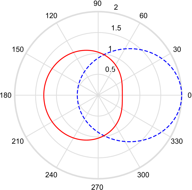
(a) $k_{0}\ell_{c}=0.5$

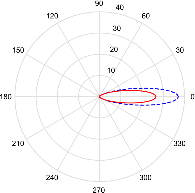
(b) $k_{0}\ell_{c}=3$

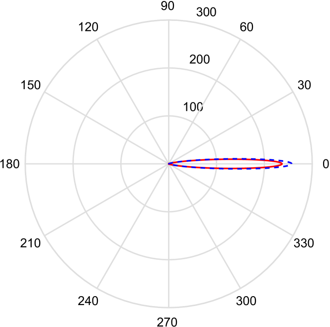
(c) $k_{0}\ell_{c}=8$

Figure 1: (Color online) Polar plots of the phase functions $f\left(\Theta\right)$ (solid line) and $f^{(\alpha\alpha)}\left(\Theta\right)$ (dashed line) for various values of $k_{0}\ell_{c}$.

\psfrag{a}[c]{}\psfrag{x}[c]{$k_{0}\ell_{c}$}\psfrag{y}[c]{$g$}\includegraphics[width=433.62pt]{Figure_g.eps}

Figure 2: (Color online) Anisotropy factor $g$ as a function of $k_{0}\ell_{c}$ when the operator contribution is (solid line) or is not (dashed line) taken into account.

Figure 2 shows that discarding the operator term has a significant impact (larger than $10\text{\,}\%$) on the anisotropy factor $g$, for frequencies such that $k_{0}\ell_{c}\lesssim 5$. In the same frequency range, it has been shown that the mean-free path $\ell_{s}$ could be nearly four times smaller than expected as $k_{0}\ell_{c}\to 0$ Baydoun et al. (2015), whereas at higher frequencies ($k_{0}\ell_{c}>10$) the scalar approximation was reasonable. Interestingly, this is not true at all for the transport mean-free path. In Fig. 3, $\ell^{*}$ is plotted as a function of frequency with and without the operator contribution. The difference is far from negligible over a much broader frequency range.

In the low-frequency regime, $1/\ell^{*}=A\sigma^{2}k_{0}^{4}\ell_{c}^{3}$, with $A=2$ (scalar case) or $A=34/3$ (operator case; as a consequence, $\ell^{*}$ is nearly six times smaller when the operator contribution is considered (the exact ratio is 17/3, for $k_{0}\ell_{c}\rightarrow 0$). As to the anisotropy factor, $g$ vanishes in the scalar case, and is equal to $-4/13$ in the operator case. Though the results were derived in the case of an exponentially-correlated disorder, interestingly the low frequency limits for $g$, $\ell_{s}$ and $\ell^{*}$ do not depend on the actual shape of the correlation function (see App. E).

At the other end of the frequency axis, $\ell_{c}/\ell^{*}\rightarrow\sigma^{2}\ln\left(k_{0}\ell_{c}\right)/2$ in both cases. But the convergence is so slow that the discrepancy persists in the high-frequency regime: it is still $30\text{\,}\%$ for $k_{0}\ell_{c}=10^{4}$! The essential reason is that for transport properties, $1-g$ matters more than $g$. Even though $g$ and $g^{\left(\alpha\alpha\right)}$ both tend to 1 (forward scattering) when $k_{0}\ell_{c}\gg 1$ (see Fig. 2) the convergence is only logarithmic, hence very slow. This can be quantified by the ratio

$$R=\dfrac{1-g}{1-g^{\left(\alpha\alpha\right)}}.$$ (47)

As soon as $k_{0}\ell_{c}\gtrsim 10$ the scattering mean-free paths $\ell_{s}$ and $\ell_{s}^{(\alpha\alpha)}$ are nearly the same, so the scalar approximation is valid to evaluate the coherent field. Thus in the high-frequency regime, we have

$$\dfrac{\ell^{*}-\ell^{*(\alpha\alpha)}}{\ell^{*}}=1-R=\dfrac{6}{1-2\ln\left(2\ k_{0}\ell_{c}\right)}.$$ (48)

If the relative error $\left|1-R\right|$ is to be kept below $\epsilon$, it implies that $k_{0}\ell_{c}$ must be larger than $\exp\left(3/\epsilon\right)/2$. For $\epsilon=0.1$ (which would still result in a significant overestimation of the transport mean-free path), this would require $k_{0}\ell_{c}$ to be larger than $5\text{\times}{10}^{12}\text{\,}$, an absurdly high value from a practical point of view. Even in a situation where a high-frequency approximation ($k_{0}\ell_{c}\gg 1$) seems reasonable (and in the case of $\ell_{s}$, the high frequency approximation does lead to $\ell_{s}^{(\alpha\alpha)}\approx\ell_{s}$ indeed as soon as $k_{0}\ell_{c}\sim 10$), it is not the case for the transport mean-free path. Of course, mathematically for $k_{0}\ell_{c}\rightarrow\infty$, we have $\ell^{*(\alpha\alpha)}=\ell^{*}$ as well, but how close to infinity does $k_{0}\ell_{c}$ have to be for the approximation to hold? At least $10^{12}$, which in practical terms means never. Moreover, it should be noted the ratio of the transport mean-free paths $\ell^{*}$ and $\ell^{*(\alpha\alpha)}$ only depend on $k_{0}\ell_{c}$, not on the fluctuation level $\sigma$. It implies that no matter how weak the fluctuations, the scalar approximation leads to incorrect results for the transport mean-free path, in an extremely broad frequency range.

\psfrag{x}[c]{$k_{0}\ell_{c}$}\psfrag{y}[c]{$\sigma^{2}\ell^{*}/\ell_{c}$}\includegraphics[width=433.62pt]{l_etoile.eps}

Figure 3: (Color online) Dimensionless transport mean-free path as a function of dimensionless frequency $k_{0}\ell_{c}$ when the operator contribution is (solid line) or is not (dashed line) taken into account.

IV.2 Numerical validation in a cubic geometry

Two numerical tools were used to validate the analytical calculations. On the one hand, the temporal wave equation [Eq. (1)] is solved using a finite-difference (FDTD) scheme for an ensemble of realizations with random spatial fluctuations of density and compressibility. In this case, heterogeneity is essentially described by two parameters: variance $\sigma^{2}$ and correlation length $\ell_{c}$. On the other hand, the Radiative Transfer Equation [Eq. (17)] is solved following a Monte Carlo approach. In this case, heterogeneity is accounted for by the phase function $f$ and the extinction and scattering lengths $\ell_{e}$ and $\ell_{s}$. The results from both approaches are compared, in order to validate the link between micro-structural parameters ($\sigma^{2}$, $\ell_{c}$) on the one hand and transport parameters ($\ell_{e}$, $\ell_{s}$ and $f$) on the other hand.

The FDTD simulations are performed using Simsonic , a software developed in our lab by Dr. E. Bossy Bossy et al. (2004). We consider a cubic domain (of length $L$) in a centered Cartesian grid $(x,y,z)$ excited by an omnidirectional point source located at $(0,0,-L/2)$. The reference (unperturbed) medium is water ($c_{0}=$1500\text{\,}\mathrm{m}\text{\,}{\mathrm{s}}^{-1}$$ and $\rho_{0}=$1000\text{\,}\mathrm{kg}\text{\,}{\mathrm{m}}^{-3}$$) and the emitted pulse has a central frequency $f_{c}=$1\text{\,}\mathrm{MHz}$$. The mesh size was $\lambda/20$, where $\lambda$ is the corresponding wavelength at the central frequency, to avoid significant numerical dispersion. In order to avoid undesired reflections, the domain is bounded by perfectly matched layers (PML). 3-D maps of the local wave speed and mass density can be designed by the user (see Ref. Baydoun et al., 2015 for more details). The cases of a full potential $\gamma$ or its scalar limit [$\beta(r)=0$] can be studied; from a practical point of view this amounts to comparing two media having the same sound speed at every point, but with or without mass density fluctuations.

A Gaussian pulse with a 1 MHz bandwidth is emitted at $t=0$ [see Fig. 4(a)], its energy is denoted by $W_{0}$. The real acoustic pressure $\operatorname{Re}p(x,y,z,t)$ and particle velocity $\operatorname{Re}\boldsymbol{\mathbf{v}}(x,y,z,t)$ are measured at $z=L/2$. Averaging the instantaneous Poynting vector over a period $T=1/f_{c}$, we have:

$$\boldsymbol{\mathbf{J}}(x,y,z,\tau) =\frac{1}{T}\int_{\tau}^{\tau+T}\operatorname{Re}p(x,y,z,t)\operatorname{Re}\boldsymbol{\mathbf{v}}(x,y,z,t)\mathrm{d}t$$ (49)

$$=\dfrac{1}{2}\operatorname{Re}\left(p(x,y,z,\tau)\boldsymbol{\mathbf{v}}^{*}(x,y,z,\tau)\right).$$ (50)

This yields the transmitted acoustic flux $\Phi$:

$$\Phi(L/2,\tau)=\int_{S}\boldsymbol{\mathbf{J}}(x,y,L/2,\tau)\cdot\mathrm{d}\boldsymbol{\mathbf{S}}.$$ (51)

$S$ is the exit face of the cube and the infinitesimal vector $\mathrm{d}\boldsymbol{\mathbf{S}}=\mathrm{dS}\boldsymbol{\mathbf{e}}_{z}$ points in the outward direction.

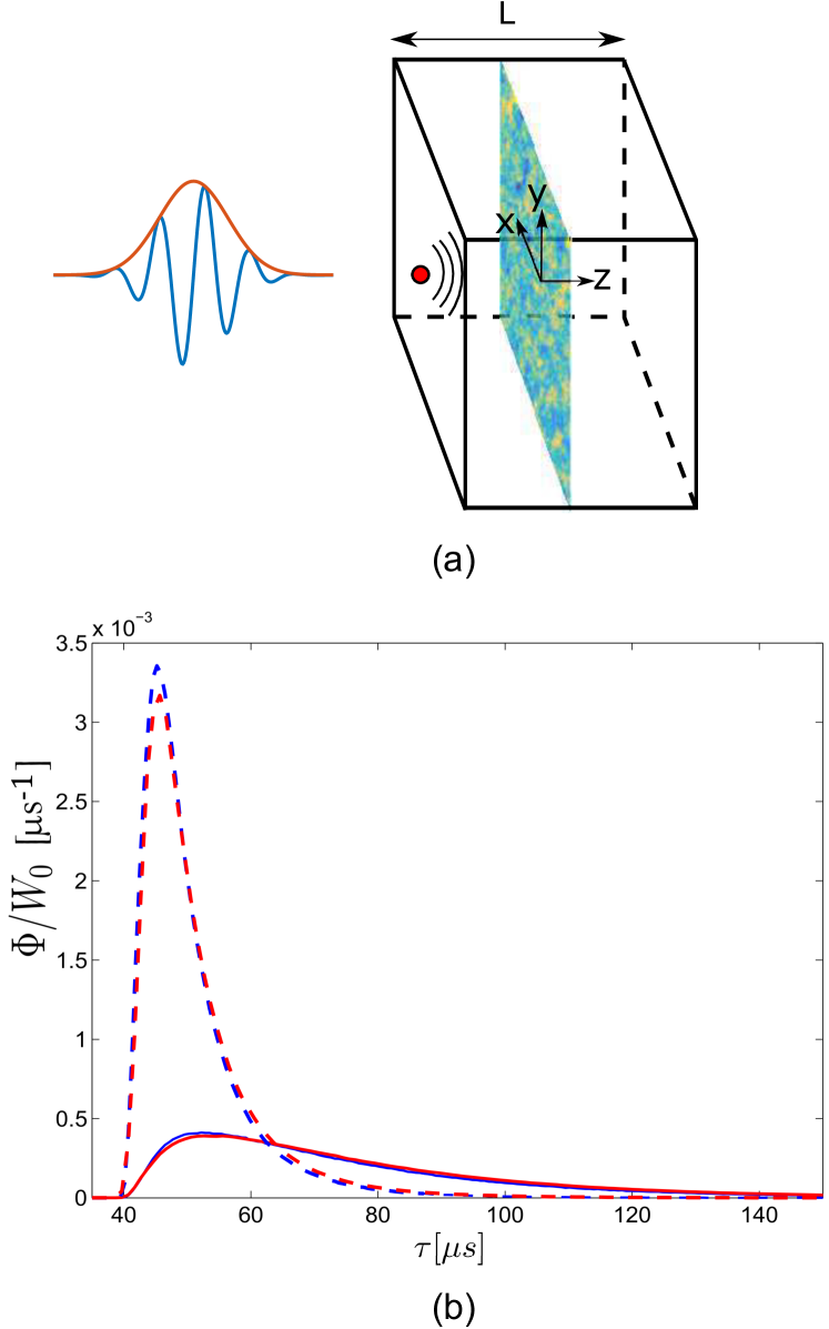
Figure 4: (Color online) Normalized acoustic flux as a function of time. (a) Sketch of the numerical experiment. The colormap represents the spatial fluctuations of the potentials $\alpha$ and $\beta$. A point source emits a Gaussian pulse with a central frequency and bandwidth of $1\text{\,}\mathrm{MHz}$ on one side of a cube of length $L=118\ell_{c}$, with $\sigma=0.15$, $\ell_{c}\sim$4.78\text{\,}\mathrm{mm}$$ hence $k_{0}\ell_{c}=2$. The exiting flux is measured on the opposite face of the cube perpendicular to $\boldsymbol{\mathbf{e}}_{z}$ at $z=L/2$. (b) Measured flux when the operator contribution is (solid line) or is not (dashed line) taken into account. The data are normalized by the energy $W_{0}$ conveyed by incident pulse. The blue and red curves are the flux calculated from FDTD and Monte Carlo simulations respectively.

As a typical example, the normalized flux $\Phi(L/2,\tau)/W_{0}$ is plotted in Fig. 4(b), for $\sigma=0.15$ and $L=118\ell_{c}$; here $\ell_{c}\sim$4.78\text{\,}\mathrm{mm}$$ hence $k_{0}\ell_{c}=2$. Interestingly, very different behaviors are observed according to whether the operator term $\beta$ is taken into account (operator) or not (scalar). Firstly the total transmission coefficients are $1.72\text{\,}\mathrm{\char 37\relax}$ (operator), and $3.84\text{\,}\mathrm{\char 37\relax}$ (scalar). Considering Fig. 4(b) as a distribution of arrival time for exiting energy packets, the average transmission times are found to be $74.9\text{\,}\mathrm{\SIUnitSymbolMicro s}$ (operator) and $50.6\text{\,}\mathrm{\SIUnitSymbolMicro s}$ (scalar), and the standard deviations are $26.9\text{\,}\mathrm{\SIUnitSymbolMicro s}$ and $8.9\text{\,}\mathrm{\SIUnitSymbolMicro s}$ respectively. Discarding the operator term makes the medium seem less opaque; this is in agreement with previous results, especially Fig. 3.

In addition, a Monte Carlo simulation of the random walk of an “acoustic particle” (a quantum of energy $W_{0}$) is performed Hammersley and Handscomb (1964); Fishman (1996). It is possible to show that this method can be used to solve the RTE exactly. At the source position, an angle is picked at random with a uniform probability distribution to mimic an omnidirectional source. The temporal profile (Gaussian envelope) is obtained by generating random departure times with a Gaussian distribution. Once it is launched, the particle propagates in a straight line over a distance $s$. $s$ is a random variable with probability density function $\exp(-s/\ell_{s})/\ell_{s}$. At this stage, the phase function $f$ is used to draw at random a new scattering direction. Then a new step length $s$ is picked up and the process is iterated. The parameters $\ell_{s}$ and $f$ were determined from Eqs. (39) and (40) with the same variance $\sigma^{2}$ and correlation length $\ell_{c}$ as in the FDTD simulation. The random walk continues as long as the particle does not

leave the domain, then another particle is launched. The transmitted flux $\Phi(\tau)$ is incremented by $W_{0}/\delta\tau$ each time a particle exits at $z=L/2$ and in the time interval $\left[\tau,\tau+\delta\tau\right]$.

$10^{8}$ particles were emitted. The resulting transmitted flux is plotted in Fig. 4 as a function of time. The Monte Carlo solution of the RTE are in very good agreement with the FDTD simulations of the wave equation, which supports the analytical derivations of $f$ and $\ell_{s}$ corresponding to Eqs. (39) and (40) presented earlier and most importantly the expression of the fundamental operators $\Sigma$ and $K$ introduced in Eqs. (28) and (30). The correspondance between the transmitted flux computed from either the time-averaged Poynting vector [Eq. (51)] or the specific intensity is established in App. D.

To obtain this good agreement, care must be taken to simultaneously fulfill the criteria of validity of the different approximations introduced in section III. First, it is necessary to ensure that $k_{0}\ell_{s}\gg 1$, to avoid localization. Here, the simulations were performed for $k_{0}\ell_{s}\sim 30$ and $k_{0}\ell_{s}^{(\alpha\alpha)}\sim 190$. Moreover, the Bourret and Ladder approximations require $(\sigma k_{0}\ell_{c})^{2}$ to be much smaller than 1 Kravtsov et al. (1989); here we took $(\sigma k_{0}\ell_{c})^{2}\sim 0.09$. Finally, in order to ensure energy conservation, we must have $k_{r}\simeq k_{0}$. In the general case, $k_{r}$ is defined implicitly [see Eq. (18)]. In App. C, the relation between $k_{r}$ and $k_{0}$ is studied in the case of an exponential disorder. In the scalar approximation, $k_{r}\simeq k_{0}$ always holds in the low-frequency (Rayleigh) regime. Interestingly, this is no longer true when the operator contribution is taken into account: there is a cutoff frequency below which $k_{r}$ significantly deviates from $k_{0}$, hence the energy conservation cannot hold in the low-frequency regime, for a finite $\sigma$. In the simulations presented here, we ensured that the condition $k_{r}\simeq k_{0}$ held, within 1 to 5 %. If the conditions mentioned above were not fulfilled, neither the analytical results nor the Monte Carlo solution would match the FDTD simulations of the wave equation.

IV.3 Plane wave transmission in a slab geometry

The operator term $\beta$ was shown to have a significant impact both on the phase function and the transport mean-free path. In this paragraph, we study the transmission of a plane wave through an infinite slab of thickness $L$. Considering that the analytical expressions for the transport parameters have been validated earlier, we now restrict ourselves to the Monte Carlo simulation to calculate the transmitted flux. Indeed, for large thicknesses $L$, full simulations of the wave equation would require much larger computational resources.

As a first example, let us consider an infinite slab of length $L=8395\ell_{c}$ in the low frequency regime ($k_{0}\ell_{c}=0.3$). For $\sigma=0.1$, the sample thickness is such that $L/\ell_{s}^{(\alpha\alpha)}=1$ and $L/\ell_{s}\simeq 3.9$. In Fig. 5, the transmitted flux is plotted as a function of time in both cases. As can be expected, when the operator contribution $\beta$ is dropped, wave transport is quasi-ballistic [$L=\ell_{s}^{(\alpha\alpha)}$]: the sample thickness is comparable to the mean-free path, scattering events are too few to significantly randomize the phases of the emerging waves. The ballistic arrival is found to convey 55% of the transmitted energy. On the contrary, if the operator contribution is considered, the transmitted intensity begins to exhibit a diffuse coda; in that case, though the ballistic peak is still visible, it only contains 8.6% of the transmitted energy.

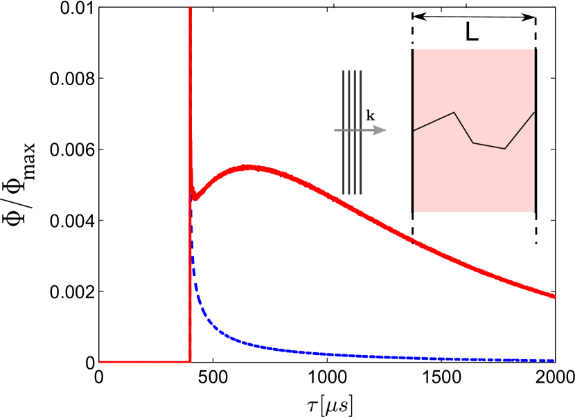
Figure 5: (Color online) Transmitted flux as a function of time in the case of an infinite slab with thickness $L=8395\ell_{c}$ ($k_{0}\ell_{c}=0.3$ and $\sigma=0.1$). The flux is computed using the Monte Carlo method, when the operator part is taken into account (solid line) or not (dashed line). Each curve is normalized by its maximum.

In order to test further the diffusive nature of sound propagation, we consider a much thicker slab. We compare the solution of the RTE to that determined by calculating the transmitted flux using the diffusion equation. Under this approximation, the tail of the transmitted flux decays exponentially as $\exp(-t/\tau_{D})$, with

$$\tau_{D}=\frac{(L+2z_{0})^{2}}{\pi^{2}D}.$$ (52)

$D=c_{\text{tr}}\ell^{*}/3$ is the diffusion constant and $z_{0}$ is the penetration depth beyond which sound starts to diffuse in the sample Durian (1994).

Energy transport can safely be considered as diffusive for samples thicker than five transport mean-free paths Zhang et al. (1999). Considering medium frequency waves ($k_{0}\ell_{c}=10$) and a weak disorder ($\sigma^{2}=10^{-4}$) such that $(k_{0}\ell_{c}\sigma)^{2}\ll 1$, the transport mean-free path is expected to be $\ell^{*}=3681\ell_{c}$ if the operator contribution is taken into account (operator), and $\ell^{*(\alpha\alpha)}=8006\ell_{c}$ under the scalar approximation (scalar). The transmitted flux (normalized to its maximum value) is plotted in Fig. 6 for $L=$8\text{\times}{10}^{4}\text{\,}$\ell_{c}$. As expected, the diffusion approximation correctly predicts the decay time of the coda. From the slope of the tail, we obtain $\tau_{D}=$0.961\text{\,}\mathrm{s}$$ (operator) and $\tau_{D}=$0.498\text{\,}\mathrm{s}$$ (scalar); the predicted values are $0.953\text{\,}\mathrm{s}$ and $0.503\text{\,}\mathrm{s}$ respectively, assuming $z_{0}\simeq 0.7\ell^{*}$ and $c_{\text{tr}}\simeq c_{0}$ Durian (1994). As a result, though the sound speed fluctuations are exactly the same in both cases the diffusion constant $D$ varies roughly by a factor of 2. Similarly, once $\ell^{*}$ or $D$ is measured from actual experimental data, inverting the result to obtain a microstructural information about $\ell_{c}$ or $\sigma$ may result in a large mistake if the scalar model is applied to the operator case. Here, using Eq. (52) we can estimate $\ell^{*}=3650\leavevmode\nobreak\ \ell_{c}$ from the measured value for $\tau_{D}$; assuming $\ell_{c}$ is known, we can invert the result, and obtain $\sigma=$1.01\text{\,}\mathrm{\char 37\relax}$$, or $\sigma=$1.49\text{\,}\mathrm{\char 37\relax}$$ under the scalar approximation (see Fig. 7). The correct value is $\sigma=$1\text{\,}\mathrm{\char 37\relax}$$ hence in this example discarding the operator term yields a $50\text{\,}\mathrm{\char 37\relax}$ error on the estimation of the fluctuations.

\psfrag{x}[c]{$\tau$ [s]}\psfrag{y}[c]{$\Phi/\Phi_{\text{max}}$}\includegraphics[width=433.62pt]{Figure6.eps}

Figure 6: (Color online) Transmitted flux as a function of time in the case of an infinite slab with thickness $L=$8\text{\times}{10}^{4}\text{\,}$\ell_{c}$ ($k_{0}\ell_{c}=10$ and $\sigma=0.01$). The flux is computed using the Monte Carlo method, when the operator part is taken into account (solid line) or not (dashed line). Each curve is normalized by its maximum. The straight lines are the asymptotes predicted by diffusion theory.

\psfrag{x}[c]{$\sigma$}\psfrag{y}[c]{$k_{0}\ell_{c}$}\includegraphics[width=433.62pt]{Inversion.eps}

Figure 7: (Color online) Solution of the inverse problem. The pairs $(\sigma,k_{0}\ell_{c})$ which are compatible with the value of $\ell^{*}$ obtained from Fig. 6 are plotted, taking into account the operator term (continuous line) or not (dashed line). The exact result ($\sigma=0.01,k_{0}\ell_{c}=10)$ is represented by a circle.

V Conclusion

In this study we have considered the transport of acoustic waves in a heterogeneous yet continuous fluid medium with both compressibility and density fluctuations. The random potential entering the wave equation for the acoustic pressure entails both a scalar and operator part, $\alpha$ and $\beta$. The scalar approximation consists in neglecting the $\beta$ contribution; in that case, the space-dependent wavespeed $c(r)$ suffices to describe heterogeneity. The main issue we addressed is the relevance of the scalar approximation when dealing with energy transport in a multiple scattering medium. The theoretical analysis we presented is based on the diagrammatic approach of multiple scattering, within Bourret and Ladder’s approximations. The self-energy and intensity operators $\Sigma$ and $K$ are expressed as a function of the correlations functions of $\alpha$ and $\beta$. This relates microstructural properties (variance and correlation lengths for $\alpha$ and $\beta$) to scattering and transport parameters. In the case of an exponentially-correlated disorder, explicit analytical expressions are derived for the scattering and extinction lengths, $\ell_{s}$ and $\ell_{e}$, transport speed $c_{\text{tr}}$ as well as the phase function, $f$. They are the constitutive parameters of the radiative transfer equation (RTE) describing wave transport in scattering media. Neglecting additional terms arising from the random operator potential $\beta$, as is usually done in the literature, was shown to have drastic consequences on the parameters of the RTE, particularly the transport mean free path, $\ell^{*}$.

For simplicity, we have focused on the case where the density fluctuations have a similar amplitude to that of the compressibility (i.e. same variance for $\alpha$ and $\beta$) and have an exponential correlation but the theoretical results of Eqs. (34) and (35) can be applied to other cases. In the simple case studied here, in the low frequency regime (i.e. when the wavelength is smaller or comparable to the correlation length) the operator term largely contributes to determine the angular distribution of the reflected waves. It was also shown to have a very strong impact on $\ell^{*}$. Its value can be down to nearly 6 times smaller than expected under the usual scalar approximation. Most importantly the error is not restricted to a given frequency range, it persists up to the very high frequency regime ($k_{0}\ell_{c}\sim$5\text{\times}{10}^{12}\text{\,}$$): no matter how weak the fluctuations, the scalar approximation leads to incorrect results for the transport mean-free path. The theoretical results presented here are supported by two types of numerical simulations: FDTD simulations of the full wave equation, and Monte Carlo solution of the radiative transfer equation.

The scattering mean-free path, the phase function, the transport mean-free path and consequently the diffusion constant and transport speed are essential parameters to characterize wave propagation in heterogeneous media. From an experimental point of view, they can be measured using coherent or incoherent transmission set-ups. To go beyond and obtain a microstuctural information about the medium (fluctuations $\sigma$, correlation length $\ell_{c}$) one has to invert the data with a model. Though the numerical examples were chosen to illustrate the theory in a rather academic situation, we have shown here that if the operator term $\beta$ is ignored, the model, and consequently the estimated values of $\sigma$ and $\ell_{c}$ may be completely wrong. The results presented here also open up interesting possibilities to investigate the influence of $\beta$ on other universal wave phenomena such as coherent backscattering.

Authorship statement

IB and DB equally contributed to this work and share the rank of first author.

Appendix A Radiative transfer equation

The appendix is dedicated to the derivation of the RTE from the Bethe-Salpeter equation. Taking advantage of Eq. (16), the spatial Fourier transform of Eq. (14) yields

$$\left\langle\widetilde{P}\left(\boldsymbol{\mathbf{k}}^{+},\omega^{+}\right)\widetilde{P}^{*}\left(\boldsymbol{\mathbf{k}}^{-},\omega^{-}\right)\right\rangle=\left\langle\widetilde{G}\left(\boldsymbol{\mathbf{k}}^{+},\omega^{+}\right)\right\rangle\left\langle\widetilde{G}^{*}\left(\boldsymbol{\mathbf{k}}^{-},\omega^{-}\right)\right\rangle\times\left\{\widetilde{S}\left(\boldsymbol{\mathbf{k}}^{+},\omega^{+}\right)\widetilde{S}^{*}\left(\boldsymbol{\mathbf{k}}^{-},\omega^{-}\right)\right.\\ \left.+\int\frac{\mathrm{d}\boldsymbol{\mathbf{k}}_{1}}{\left(2\pi\right)^{3}}\left\langle\widetilde{P}\left(\boldsymbol{\mathbf{k}}_{1}+\frac{\boldsymbol{\mathbf{q}}}{2},\omega^{+}\right)\widetilde{P}^{*}\left(\boldsymbol{\mathbf{k}}_{1}-\frac{\boldsymbol{\mathbf{q}}}{2},\omega^{-}\right)\right\rangle\widetilde{\varGamma}\left(\boldsymbol{\mathbf{k}}^{+},\boldsymbol{\mathbf{k}}^{-},\boldsymbol{\mathbf{k}}_{1}+\frac{\boldsymbol{\mathbf{q}}}{2},\boldsymbol{\mathbf{k}}_{1}-\frac{\boldsymbol{\mathbf{q}}}{2},\omega^{+},\omega^{-}\right)\right\}.$$ (53)

In the equation above we have used the notations $\boldsymbol{\mathbf{k}}^{\pm}=\boldsymbol{\mathbf{k}}\pm\boldsymbol{\mathbf{q}}/2$, $\boldsymbol{\mathbf{k}}_{1}^{\pm}=\boldsymbol{\mathbf{k}}_{1}\pm\boldsymbol{\mathbf{q}}/2$ and $\omega^{\pm}=\omega\pm\Omega/2$. The average Green function is expressed as

$$\left\langle\widetilde{G}\left(\boldsymbol{\mathbf{k}}\right)\right\rangle=\frac{1}{k_{0}^{2}-k^{2}-\widetilde{\Sigma}\left(\boldsymbol{\mathbf{k}},\omega\right)}$$ (54)

and since $AB=\left(A-B\right)/\left(B^{-1}-A^{-1}\right)$ we obtain the following form of the Bethe-Salpeter equation

$$\left[\frac{\Omega\omega}{c_{0}^{2}}-\boldsymbol{\mathbf{k}}\cdot\boldsymbol{\mathbf{q}}-\widetilde{\Sigma}\left(\boldsymbol{\mathbf{k}}^{+},\omega^{+}\right)+\widetilde{\Sigma}^{*}\left(\boldsymbol{\mathbf{k}}^{-},\omega^{-}\right)\right]\left\langle\widetilde{P}\left(\boldsymbol{\mathbf{k}}^{+},\omega^{+}\right)\widetilde{P}^{*}\left(\boldsymbol{\mathbf{k}}^{-},\omega^{-}\right)\right\rangle\\ =\left[\left\langle\widetilde{G}\left(\boldsymbol{\mathbf{k}}^{+},\omega^{+}\right)\right\rangle-\left\langle\widetilde{G}^{*}\left(\boldsymbol{\mathbf{k}}^{-},\omega^{-}\right)\right\rangle\right]\left\{\widetilde{S}\left(\boldsymbol{\mathbf{k}}^{+},\omega^{+}\right)\widetilde{S}^{*}\left(\boldsymbol{\mathbf{k}}^{-},\omega^{-}\right)\right.\\ \left.+\int\frac{\mathrm{d}\boldsymbol{\mathbf{k}}_{1}}{\left(2\pi\right)^{3}}\left\langle\widetilde{P}\left(\boldsymbol{\mathbf{k}}_{1}+\frac{\boldsymbol{\mathbf{q}}}{2},\omega^{+}\right)\widetilde{P}^{*}\left(\boldsymbol{\mathbf{k}}_{1}-\frac{\boldsymbol{\mathbf{q}}}{2},\omega^{-}\right)\right\rangle\widetilde{\varGamma}\left(\boldsymbol{\mathbf{k}}+\frac{\boldsymbol{\mathbf{q}}}{2},\boldsymbol{\mathbf{k}}^{-},\boldsymbol{\mathbf{k}}_{1}+\frac{\boldsymbol{\mathbf{q}}}{2},\boldsymbol{\mathbf{k}}_{1}-\frac{\boldsymbol{\mathbf{q}}}{2},\omega^{+},\omega^{-}\right)\right\}.$$ (55)

The above equation is still exact. To derive the RTE, three assumptions are necessary:

• (H₁): Separation of scales in time and space. From a physical point of view, this means that the scattered wavefield $p$ has a typical duration $\Delta T$ much larger than the average period $2\pi/\omega$, and a typical spatial extent $\Delta x$ much larger than the average wavelength $2\pi/k_{0}$. In other words, at any point (respectively, at any time) the wave field $p$ shows rapid temporal (spatial) oscillations, modulated by a slowly varying envelope. Reciprocally, in Fourier space, (H₁) implies that $\left\langle\widetilde{P}\left(\boldsymbol{\mathbf{k}}+\boldsymbol{\mathbf{q}}/2),\omega+\Omega/2\right)\widetilde{P}^{*}\left(\boldsymbol{\mathbf{k}}-\boldsymbol{\mathbf{q}}/2,\omega-\Omega/{2}\right)\right\rangle$ shows the same property. The variations of $\boldsymbol{\mathbf{q}}$ around $\boldsymbol{\mathbf{k}}$ are limited to $\pm q_{\text{max}}=\pm 2\pi/\Delta x\ll k$ and the variations of $\Omega$ around $\omega$ are limited to $\pm\Omega_{\text{max}}=\pm 2\pi/\Delta T\ll\omega$.

• (H₂): Weak dispersion of transport parameters. The self-energy and intensity operators are supposed to vary slowly enough with angular frequency $\omega$ and wavenumber $k$, so that they can be considered as constant at the scale of $q_{\text{max}}$ and $\Omega_{\text{max}}$.

• (H₃): Weak disorder assumption. It is assumed that $\operatorname{Im}\widetilde{\Sigma}\left(\boldsymbol{\mathbf{k}},\omega\right)\ll\operatorname{Re}\left[k_{0}^{2}-\widetilde{\Sigma}\left(\boldsymbol{\mathbf{k}},\omega\right)\right]$. In a homogeneous medium, the so-called spectral function $\operatorname{Im}\widetilde{G_{0}}$ has a singularity at $k_{0}=\omega/c_{0}$. (H₃) means that $\operatorname{Im}\left\langle\widetilde{G}\right\rangle$, even if it does not have a true singularity, is still strongly peaked around a well-defined line in the $(\omega,\boldsymbol{\mathbf{k}})$ plane, so that at any frequency a single effective wavenumber can be defined. In other words, the self-energy is a local operator. (H₃) can be interpreted as a weak fluctuation hypothesis, since it limits the allowed values for $\sigma$ (see App. C).

If we were to perform a temporal ($\Omega\rightarrow\tau$) and spatial ($\boldsymbol{\mathbf{q}}\rightarrow\boldsymbol{\mathbf{r}}$) Fourier transform of Eq. (55), because of (H₁) and (H₂) we could do the following replacements under the Fourier integral:

$$\tilde{\Sigma}\left(\boldsymbol{\mathbf{k}}^{\pm},\omega^{\pm}\right) \simeq\tilde{\Sigma}\left(\boldsymbol{\mathbf{k}},\omega\right),$$ (56)

$$\widetilde{\varGamma}\left(\boldsymbol{\mathbf{k}}^{+},\boldsymbol{\mathbf{k}}^{-},\boldsymbol{\mathbf{k}}_{1}+\frac{\boldsymbol{\mathbf{q}}}{2},\boldsymbol{\mathbf{k}}_{1}-\frac{\boldsymbol{\mathbf{q}}}{2},\omega^{+},\omega^{-}\right)$$

$$\simeq\widetilde{\varGamma}\left(\boldsymbol{\mathbf{k}},\boldsymbol{\mathbf{k}},\boldsymbol{\mathbf{k}}_{1},\boldsymbol{\mathbf{k}}_{1},\omega,\omega\right),$$ (57)

$$\left\langle\widetilde{G}\left(\boldsymbol{\mathbf{k}}^{\pm},\omega^{\pm}\right)\right\rangle \simeq\left\langle\widetilde{G}\left(\boldsymbol{\mathbf{k}},\omega\right)\right\rangle.$$ (58)

Moreover, in the sense of distributions, we have

$$\lim_{\varepsilon\rightarrow 0^{+}}\frac{1}{x-x_{0}+j\varepsilon}=\operatorname{VP}\frac{1}{x-x_{0}}-j\pi\delta\left(x-x_{0}\right),$$ (59)

where $\operatorname{VP}$ stands for the Cauchy principal value. Hence, using (H₃), the spectral function may be written

$$\operatorname{Im}\left\langle\widetilde{G}\left(\boldsymbol{\mathbf{k}},\omega\right)\right\rangle=-\pi\delta\left[k_{0}^{2}-k^{2}-\operatorname{Re}\tilde{\Sigma}\left(\boldsymbol{\mathbf{k}},\omega\right)\right].$$ (60)

The Dirac delta function imposes that the modulus $k$ of the wave-vector $\boldsymbol{\mathbf{k}}$ must be equal to $k_{r}$, with

$$k_{r}=\sqrt{k_{0}^{2}-\operatorname{Re}\tilde{\Sigma}\left(k_{r},\omega\right)}.$$ (61)

As a result, again, if we were to perform a temporal ($\Omega\rightarrow\tau$) and spatial ($\boldsymbol{\mathbf{q}}\rightarrow\boldsymbol{\mathbf{r}}$) Fourier transform of Eq. (55), the integrand could be replaced by

$$\left[\frac{\Omega\omega}{c_{0}^{2}}-\boldsymbol{\mathbf{k}}\cdot\boldsymbol{\mathbf{q}}-j\operatorname{Im}\widetilde{\Sigma}\left(\boldsymbol{\mathbf{k}},\omega\right)\right]\left\langle\widetilde{P}\left(\boldsymbol{\mathbf{k}}+\frac{\boldsymbol{\mathbf{q}}}{2},\omega+\frac{\Omega}{2}\right)\widetilde{P}^{*}\left(\boldsymbol{\mathbf{k}}-\frac{\boldsymbol{\mathbf{q}}}{2},\omega-\frac{\Omega}{2}\right)\right\rangle=j\pi\delta\left[k^{2}-k_{0}^{2}-\operatorname{Re}\tilde{\Sigma}\left(\boldsymbol{\mathbf{k}},\omega\right)\right]\\ \times\left\{\widetilde{S}\left(\boldsymbol{\mathbf{k}}+\frac{\boldsymbol{\mathbf{q}}}{2},\omega+\frac{\Omega}{2}\right)\widetilde{S}^{*}\left(\boldsymbol{\mathbf{k}}-\frac{\boldsymbol{\mathbf{q}}}{2},\omega-\frac{\Omega}{2}\right)+\int\frac{\mathrm{d}\boldsymbol{\mathbf{k}}_{1}}{\left(2\pi\right)^{3}}\left\langle\widetilde{P}\left(\boldsymbol{\mathbf{k}}_{1}+\frac{\boldsymbol{\mathbf{q}}}{2},\omega+\frac{\Omega}{2}\right)\widetilde{P}^{*}\left(\boldsymbol{\mathbf{k}}_{1}-\frac{\boldsymbol{\mathbf{q}}}{2},\omega-\frac{\Omega}{2}\right)\right\rangle\right.\\ \times\left.\vphantom{\frac{\mathrm{d}\boldsymbol{\mathbf{k}}_{1}}{\left(2\pi\right)^{3}}}\widetilde{\varGamma}\left(\boldsymbol{\mathbf{k}},\boldsymbol{\mathbf{k}},\boldsymbol{\mathbf{k}}_{1},\boldsymbol{\mathbf{k}}_{1},\omega,\omega\right)\right\}.$$ (62)

We now define a quantity $\mathcal{L}\left(\boldsymbol{\mathbf{q}},\hat{\boldsymbol{\mathbf{k}}},\Omega,\omega\right)$ such that

$$\frac{8\pi^{3}}{k_{r}^{2}}\delta\left[k-k_{r}\right]\mathcal{L}\left(\boldsymbol{\mathbf{q}},\hat{\boldsymbol{\mathbf{k}}},\Omega,\omega\right)\\ =\left\langle\widetilde{P}\left(k_{r}\hat{\boldsymbol{\mathbf{k}}}+\frac{\boldsymbol{\mathbf{q}}}{2},\omega+\frac{\Omega}{2}\right)\widetilde{P}^{*}\left(k_{r}\hat{\boldsymbol{\mathbf{k}}}-\frac{\boldsymbol{\mathbf{q}}}{2},\omega-\frac{\Omega}{2}\right)\right\rangle.$$ (63)

The temporal ($\Omega\rightarrow\tau$) and spatial ($\boldsymbol{\mathbf{q}}\rightarrow\boldsymbol{\mathbf{r}}$) Fourier transform of Eq. (63) yields

$$\frac{8\pi^{3}}{k_{r}^{2}}\delta\left[k-k_{r}\right]\mathcal{I}\left(\boldsymbol{\mathbf{r}},\hat{\boldsymbol{\mathbf{k}}},\tau,\omega\right)\\ =\int\left\langle\widetilde{P}\left(k_{r}\hat{\boldsymbol{\mathbf{k}}}+\frac{\boldsymbol{\mathbf{q}}}{2},\omega+\frac{\Omega}{2}\right)\widetilde{P}^{*}\left(k_{r}\hat{\boldsymbol{\mathbf{k}}}-\frac{\boldsymbol{\mathbf{q}}}{2},\omega-\frac{\Omega}{2}\right)\right\rangle\\ \times\exp\left[j\boldsymbol{\mathbf{q}}\cdot\boldsymbol{\mathbf{r}}-j\Omega\tau\right]\frac{\mathrm{d}\boldsymbol{\mathbf{q}}}{8\pi^{3}}\frac{\mathrm{d}\Omega}{2\pi}.\\ =\int\left\langle p\left(\boldsymbol{\mathbf{r}}+\frac{\boldsymbol{\mathbf{\uprho}}}{2},\tau+\frac{t}{2}\right)p^{*}\left(\boldsymbol{\mathbf{r}}-\frac{\boldsymbol{\mathbf{\uprho}}}{2},\tau-\frac{t}{2}\right)\right\rangle\\ \times\exp\left[-j\boldsymbol{\mathbf{k}}\cdot\boldsymbol{\mathbf{\uprho}}+j\omega t\right]\mathrm{d}\boldsymbol{\mathbf{\uprho}}\mathrm{d}t.$$ (64)

Equation (64) defines the specific intensity $\mathcal{I}\left(\boldsymbol{\mathbf{r}},\hat{\boldsymbol{\mathbf{k}}},\tau,\omega\right)$ as the spatial and temporal Fourier transform of $\mathcal{L}$, and equivalently as the Wigner transform of the wavefield $p$. In the phenomenological approach of RTE, $\mathcal{I}$ is introduced ad hoc as a directional decomposition (along $\boldsymbol{\mathbf{\hat{k}}}$) of the power density per unit area (as a function of $\boldsymbol{\mathbf{r}}$, $\tau$ and $\omega$), expressed in $\mathrm{W}\text{\,}{\mathrm{m}}^{-2}\text{\,}{\mathrm{sr}}^{-1}$, with no explicit relation to the wavefield. The Wigner transform allows a rigorous and unambiguous mathematical definition of $\mathcal{I}$. It should be emphasized that though the Wigner transform of the wavefield can always be defined and calculated, it can be physically interpreted as a power spectral density only if (H₁) and (H₃) are valid, and $p(\boldsymbol{\mathbf{r}},\tau)$ denotes the complex-valued analytical signal associated to the real acoustic pressure.

Finally, taking the spatio-temporal Fourier transform ($\Omega\rightarrow\tau,\boldsymbol{\mathbf{q}}\rightarrow\boldsymbol{\mathbf{r}}$) of Eq. (62) and inserting Eq. (63) leads to Eq. (17).

Appendix B Ward identity and energy conservation

In the main text, we have shown that energy conservation is fulfilled under the Bourret and Ladder approximations for the self energy $\Sigma$ and the vertex intensity $K$, as long as $k_{r}=k_{0}$. In this Appendix, we show how to adapt the Bourret approximation to ensure energy conservation even if $k_{r}\neq k_{0}$. This derivation is adapted from Ref. Kuhn et al., 2007. We consider the most general case of a reciprocal and non-local potential $V(\boldsymbol{\mathbf{r}},\boldsymbol{\mathbf{r}}^{\prime})$. In the Ladder approximation, the vertex intensity is still given by Eq. (26). Using Eq. (21), this leads to the following expression of the scattering coefficient:

$$\frac{1}{\ell_{s}(\omega)}=\frac{k_{0}^{4}}{16\pi^{2}}\int\widetilde{C}(k_{r}\hat{\boldsymbol{\mathbf{k}}},k_{r}\hat{\boldsymbol{\mathbf{k}}},k_{r}\hat{\boldsymbol{\mathbf{q}}},k_{r}\hat{\boldsymbol{\mathbf{q}}})\mathrm{d}\Omega_{\hat{\boldsymbol{\mathbf{q}}}}$$ (65)

where the correlation function $\widetilde{C}$ is defined as

$$\widetilde{C}(\boldsymbol{\mathbf{k}},\boldsymbol{\mathbf{k}}^{\prime},\boldsymbol{\mathbf{q}},\boldsymbol{\mathbf{q}}^{\prime})=8\pi^{3}\delta(\boldsymbol{\mathbf{k}}-\boldsymbol{\mathbf{k}}^{\prime}-\boldsymbol{\mathbf{q}}+\boldsymbol{\mathbf{q}}^{\prime})\left\langle V(\boldsymbol{\mathbf{k}},\boldsymbol{\mathbf{q}})V(\boldsymbol{\mathbf{k}}^{\prime},\boldsymbol{\mathbf{q}}^{\prime})\right\rangle$$ (66)

because of translational invariance (i.e. statistical homogeneity of the system). Regarding the self-energy, we modify the Bourret approximation given by Eq. (25) by replacing the free-space Green function by the average one. This leads to the following closed equation:

$$\Sigma\left(\boldsymbol{\mathbf{r}}_{1},\boldsymbol{\mathbf{r}}_{2}\right)\approx k_{0}^{4}\int\mathrm{d}\boldsymbol{\mathbf{\uprho}}_{1}\mathrm{d}\boldsymbol{\mathbf{\uprho}}_{2}\left\langle G\left(\boldsymbol{\mathbf{\uprho}}_{1},\boldsymbol{\mathbf{\uprho}}_{2}\right)\right\rangle\\ \times\left\langle V\left(\boldsymbol{\mathbf{r}}_{1},\boldsymbol{\mathbf{\uprho}}_{1}\right)V\left(\boldsymbol{\mathbf{\uprho}}_{2},\boldsymbol{\mathbf{r}}_{2}\right)\right\rangle$$ (67)

which reads in the Fourier domain

$$\widetilde{\Sigma}\left(\boldsymbol{\mathbf{k}}\right)=k_{0}^{4}\int\operatorname{Im}\left\langle G(\boldsymbol{\mathbf{q}})\right\rangle\widetilde{C}(\boldsymbol{\mathbf{k}},\boldsymbol{\mathbf{k}},\boldsymbol{\mathbf{q}},\boldsymbol{\mathbf{q}})\frac{\mathrm{d}\boldsymbol{\mathbf{q}}}{8\pi^{3}}.$$ (68)

Making use of Eq. (60), we finally get

$$\frac{1}{\ell_{e}(\omega)}=\frac{k_{0}^{4}}{16\pi^{2}}\int\widetilde{C}(k_{r}\hat{\boldsymbol{\mathbf{k}}},k_{r}\hat{\boldsymbol{\mathbf{k}}},k_{r}\hat{\boldsymbol{\mathbf{q}}},k_{r}\hat{\boldsymbol{\mathbf{q}}})\mathrm{d}\Omega_{\hat{\boldsymbol{\mathbf{q}}}}$$ (69)

which leads to $\ell_{s}(\omega)=\ell_{e}(\omega)$, hence energy conservation. In the present study, we have limited $k_{0}\ell_{c}$ and $\sigma$ to a range where $k_{r}\simeq k_{0}$ in order to have explicit expressions for the transport parameters. Yet it should be noted that the validity of the RTE is not restricted to this case and energy conservation can be fulfilled even if $k_{r}\neq k_{0}$.

Appendix C $k_{r}$ versus $k_{0}$

The particular wavenumber $k_{r}$ is determined by the condition

$$k_{r}^{2}=\operatorname{Re}\left[k_{0}^{2}-\widetilde{\Sigma}\left(k_{r},\omega\right)\right].$$ (70)

In the literature, it is usually assumed that $k_{r}\approx k_{0}$. This was done in Section III to determine an expression for the transport coefficients of the RTE. In this appendix, we briefly show that this can be justified at all frequencies as long as $\sigma$ is weak, under the scalar approximation. Interestingly, this is not true when the operator contribution $\beta$ is taken into account: in that case, no matter how small $\sigma$ is, as long as it is finite there is a cut-off frequency under which $k_{r}\approx k_{0}$ does not hold.

In the case of an exponentially-correlated disorder and provided that the free-space Green function is used in the Bourret approximation, it is straightforward to calculate the spatial Fourier transform of the self-energy with Eqs. (28) and (29) Baydoun et al. (2015). Hence two implicit and approximate expressions for Eq. (70) can be derived. In the general case, we obtain:

$$\left(k_{r}\ell_{c}\right)^{2}=\left(k_{0}\ell_{c}\right)^{2}\\ +\sigma^{2}\frac{\left(k_{0}\ell_{c}\right)^{4}\left[\left(k_{r}\ell_{c}\right)^{2}+1-\left(k_{0}\ell_{c}\right)^{2}\right]-2\left(k_{0}\ell_{c}\right)^{2}}{\left[\left(k_{r}\ell_{c}\right)^{2}+1-\left(k_{0}\ell_{c}\right)^{2}\right]^{2}+4\left(k_{0}\ell_{c}\right)^{2}}\\ -\sigma^{2}\frac{1-2\left(k_{0}\ell_{c}\right)^{2}}{2k_{r}\ell_{c}}\left[\arctan\left(k_{0}\ell_{c}+k_{r}\ell_{c}\right)\right.\\ \left.-\arctan\left(k_{0}\ell_{c}-k_{r}\ell_{c}\right)\right].$$ (71)

And under the scalar approximation:

$$\left[k_{r}^{(\alpha\alpha)}\ell_{c}\right]^{2}=\left(k_{0}\ell_{c}\right)^{2}\\ +\sigma^{2}\frac{\left(k_{0}\ell_{c}\right)^{4}\left[\left(k_{r}\ell_{c}\right)^{2}+1-\left(k_{0}\ell_{c}\right)^{2}\right]}{\left[\left(k_{r}\ell_{c}\right)^{2}+1-\left(k_{0}\ell_{c}\right)^{2}\right]^{2}+4\left(k_{0}\ell_{c}\right)^{2}}.$$ (72)

\psfrag{x}[c]{$k_{0}\ell_{c}$}\psfrag{y}[c]{${k_{r}}/{k_{0}}$}\includegraphics[width=433.62pt]{Figure_kr.eps}

Figure 8: (Color online) Ratio between $k_{r}$ and $k_{0}$, for $\sigma=0.1$ in the scalar (dashed line) and operator (solid line) cases. At this level of fluctuation, $k_{0}$ and $k_{r}$ are indistinguishable in the scalar case. On the contrary, in the operator case the low frequency-regime becomes clearly incompatible with the approximation $k_{r}\approx k_{0}$ as frequency diminishes, until Eq. (71) has no longer a real solution for $k_{0}\ell_{c}<0.0995$.

Equation (72) always has a real solution. In the low frequency ($k_{0}\ell_{c}\ll 1$) and low fluctuation ($\sigma\ll 1$) approximations, it yields $k_{r}^{(\alpha\alpha)}=k_{0}(1+\sigma^{2}k_{0}^{4}\ell_{c}^{4})\approx k_{0}$. On the contrary for Eq. (71) to have a real solution, $k_{0}\ell_{c}$ must be above a certain threshold. In the low frequency regime, with a Taylor expansion, we find that the cut-off is approximately at $k_{0}\ell_{c}=\sigma$. For instance, with $\sigma=0.1$, $k_{r}\approx k_{0}$ is only valid (within 5%) if $k_{0}\ell_{c}>0.3$. The existence of a threshold and the difference between the operator case and the scalar approximation is illustrated in Fig. 8. The low-frequency limit (Rayleigh regime) should be handled with care in the operator case: for a finite fluctuation level $\sigma$, the $k_{r}\approx k_{0}$ approximation fails below the cut-off frequency, and the analytical expressions for transport parameters are inapplicable. Results obtained in the Rayleigh regime are meaningful only if one makes $\sigma$ tend to zero as $k_{0}\ell_{c}$ does.

Appendix D Wigner Transform and Poynting vector

From the specific intensity $\mathcal{I}$, the average current of “acoustic particles” may be represented by the vector

$$\boldsymbol{\mathbf{J}}_{\mathcal{I}}\left(\boldsymbol{\mathbf{r}},\tau,\omega\right)=\int_{4\pi}\mathcal{I}\left(\boldsymbol{\mathbf{r}},\boldsymbol{\mathbf{\hat{q}}},\tau,\omega\right)\boldsymbol{\mathbf{\hat{q}}}\mathrm{d}\boldsymbol{\mathbf{\hat{q}}}.$$ (73)

Using the properties of the Dirac distribution and since $\boldsymbol{\mathbf{q}}=q\boldsymbol{\mathbf{\hat{q}}}$, $\boldsymbol{\mathbf{J}}_{\mathcal{I}}$ may be rewritten

$$\boldsymbol{\mathbf{J}}_{\mathcal{I}}\left(\boldsymbol{\mathbf{r}},\tau,\omega\right)=\dfrac{1}{k_{r}^{3}}\int_{4\pi}\delta\left[q-k_{r}\right]\mathcal{I}\left(\boldsymbol{\mathbf{r}},\boldsymbol{\mathbf{\hat{q}}},\tau,\omega\right)\boldsymbol{\mathbf{q}}\mathrm{d}\boldsymbol{\mathbf{q}}.$$ (74)

The definition of the specific intensity [Eq. (64)] yields

$$\boldsymbol{\mathbf{J}}_{\mathcal{I}}\left(\boldsymbol{\mathbf{r}},\tau,\omega\right)=\\ \dfrac{1}{8\pi^{3}k_{r}}\int\left\langle p\left(\boldsymbol{\mathbf{r}}+\frac{\boldsymbol{\mathbf{\uprho}}}{2},\tau+\frac{t}{2}\right)p^{*}\left(\boldsymbol{\mathbf{r}}-\frac{\boldsymbol{\mathbf{\uprho}}}{2},\tau-\frac{t}{2}\right)\right\rangle\\ \times\exp\left[-j\boldsymbol{\mathbf{q}}\cdot\boldsymbol{\mathbf{\uprho}}+j\omega t\right]\boldsymbol{\mathbf{q}}\mathrm{d}\boldsymbol{\mathbf{q}}\mathrm{d}\boldsymbol{\mathbf{\uprho}}\mathrm{d}t.$$

Since $\boldsymbol{\mathbf{q}}\exp\left[-j\boldsymbol{\mathbf{q}}\cdot\boldsymbol{\mathbf{\uprho}}\right]=j\boldsymbol{\mathbf{\nabla}}_{\boldsymbol{\mathbf{\uprho}}}\exp\left[-j\boldsymbol{\mathbf{q}}\cdot\boldsymbol{\mathbf{\uprho}}\right]$, an integration by part over $\boldsymbol{\mathbf{\rho}}$ leads to

$$\boldsymbol{\mathbf{J}}_{\mathcal{I}}\left(\boldsymbol{\mathbf{r}},\tau,\omega\right)=-j\dfrac{1}{8\pi^{3}k_{r}}\\ \times\int\boldsymbol{\mathbf{\nabla}}_{\boldsymbol{\mathbf{\uprho}}}\left[\left\langle p\left(\boldsymbol{\mathbf{r}}+\frac{\boldsymbol{\mathbf{\uprho}}}{2},\tau+\frac{t}{2}\right)p^{*}\left(\boldsymbol{\mathbf{r}}-\frac{\boldsymbol{\mathbf{\uprho}}}{2},\tau-\frac{t}{2}\right)\right\rangle\right]\\ \times\exp\left[-j\boldsymbol{\mathbf{q}}\cdot\boldsymbol{\mathbf{\uprho}}+j\omega t\right]\mathrm{d}\boldsymbol{\mathbf{q}}\mathrm{d}\boldsymbol{\mathbf{\uprho}}\mathrm{d}t.$$

Besides,

$$\boldsymbol{\mathbf{\nabla}}_{\boldsymbol{\mathbf{\uprho}}}p\left(\boldsymbol{\mathbf{r}}\pm\frac{\boldsymbol{\mathbf{\uprho}}}{2},\tau+\frac{t}{2}\right)=\pm\frac{1}{2}\boldsymbol{\mathbf{\nabla}}_{\boldsymbol{\mathbf{r}}}p\left(\boldsymbol{\mathbf{r}}\pm\frac{\boldsymbol{\mathbf{\uprho}}}{2},\tau+\frac{t}{2}\right)$$

hence

$$\boldsymbol{\mathbf{J}}_{\mathcal{I}}\left(\boldsymbol{\mathbf{r}},\tau,\omega\right)=\dfrac{1}{8\pi^{3}k_{r}}\\ \times\int\operatorname{Im}\left\langle\boldsymbol{\mathbf{\nabla}}_{\boldsymbol{\mathbf{r}}}\left[p\left(\boldsymbol{\mathbf{r}}+\frac{\boldsymbol{\mathbf{\uprho}}}{2},\tau+\frac{t}{2}\right)\right]p^{*}\left(\boldsymbol{\mathbf{r}}-\frac{\boldsymbol{\mathbf{\uprho}}}{2},\tau-\frac{t}{2}\right)\right\rangle\\ \times\exp\left[-j\boldsymbol{\mathbf{q}}\cdot\boldsymbol{\mathbf{\uprho}}+j\omega t\right]\mathrm{d}\boldsymbol{\mathbf{q}}\mathrm{d}\boldsymbol{\mathbf{\uprho}}\mathrm{d}t.$$

The integation over $\boldsymbol{\mathbf{\uprho}}$ is straightforward, since

$$\dfrac{1}{8\pi^{3}}\int\exp\left[-j\boldsymbol{\mathbf{q}}\cdot\boldsymbol{\mathbf{\uprho}}\right]\mathrm{d}\boldsymbol{\mathbf{q}}=\delta(\boldsymbol{\mathbf{\uprho}}),$$

hence:

$$\boldsymbol{\mathbf{J}}_{\mathcal{I}}\left(\boldsymbol{\mathbf{r}},\tau,\omega\right)=\\ \dfrac{1}{k_{r}}\int\operatorname{Im}\left\langle\boldsymbol{\mathbf{\nabla}}_{\boldsymbol{\mathbf{r}}}\left[p\left(\boldsymbol{\mathbf{r}},\tau+\frac{t}{2}\right)\right]p^{*}\left(\boldsymbol{\mathbf{r}},\tau-\frac{t}{2}\right)\right\rangle\\ \times\exp\left[j\omega t\right]\mathrm{d}\boldsymbol{\mathbf{\uprho}}\mathrm{d}t.$$

Next, we integrate over frequency and obtain

$$\int\boldsymbol{\mathbf{J}}_{\mathcal{I}}\left(\boldsymbol{\mathbf{r}},\tau,\omega\right)\mathrm{d}\omega=\\ \dfrac{2\pi}{k_{r}}\operatorname{Im}\left\langle\boldsymbol{\mathbf{\nabla}}\left[p\left(\boldsymbol{\mathbf{r}},\tau\right)\right]p^{*}\left(\boldsymbol{\mathbf{r}},\tau\right)\right\rangle.$$

At this stage, we can relate $\boldsymbol{\mathbf{J}}_{\mathcal{I}}$ to $\boldsymbol{\mathbf{J}}$, the time-averaged acoustic Poynting vector [Eq. (49)] since $\boldsymbol{\mathbf{\nabla}}\left[p\left(\boldsymbol{\mathbf{r}},\tau\right)\right]=j\omega\rho(\boldsymbol{\mathbf{r}})\boldsymbol{\mathbf{v}}\left(\boldsymbol{\mathbf{r}},\tau\right)$:

$$\int\boldsymbol{\mathbf{J}}_{\mathcal{I}}\left(\boldsymbol{\mathbf{r}},\tau,\omega\right)\mathrm{d}\omega=\\ \dfrac{4\pi\omega}{k_{r}}\left\langle\rho(\boldsymbol{\mathbf{r}})\boldsymbol{\mathbf{J}}\left(\boldsymbol{\mathbf{r}},\tau\right)\right\rangle.$$ (75)

Next, $k_{r}$ is approximated by $k_{0}$, as usual. Furthermore, in the FDTD numerical simulation, the exiting flux was measured just behind the slab ($z=L/2^{+}$), in a homogenous region: in that case $\rho$ can be taken out of the bracket in Eq. (75), to obtain

$$\int\boldsymbol{\mathbf{J}}_{\mathcal{I}}\left(\boldsymbol{\mathbf{r}},\tau,\omega\right)\mathrm{d}\omega=\\ 4\pi\rho_{0}c_{0}\left\langle\boldsymbol{\mathbf{J}}\left(\boldsymbol{\mathbf{r}},\tau\right)\right\rangle.$$ (76)

Hence, apart from a multiplicative constant with the dimensions of an acoustic impedance, the directional average of the specific intensity (current of “acoustic particles”) can be identified to the frequency-averaged Poynting vector ($\mathrm{W}\text{\,}{\mathrm{m}}^{-2}$).

Note that if the exiting flux was not measured outside of the slab, the relation between $\boldsymbol{\mathbf{J}}_{\mathcal{I}}$ and $\boldsymbol{\mathbf{J}}$ would only be approximate, assuming $\left\langle\rho(\boldsymbol{\mathbf{r}})\boldsymbol{\mathbf{J}}\left(\boldsymbol{\mathbf{r}},\tau\right)\right\rangle\approx\left\langle\rho(\boldsymbol{\mathbf{r}})\right\rangle\left\langle\boldsymbol{\mathbf{J}}\left(\boldsymbol{\mathbf{r}},\tau\right)\right\rangle.$

Appendix E Low and high-frequency limits of $g$

Assuming that the correlation functions $C_{\alpha\alpha}$,$C_{\alpha\beta}$ and $C_{\beta\beta}$ are identical, Eq. (35) yields

$$f^{(\alpha\alpha)}\left(\cos\Theta,\omega\right) =\frac{k_{0}^{4}\ell_{s}^{(\alpha\alpha)}}{4\pi}\widetilde{C}\left[2k_{0}\left(1-\cos\Theta\right)\right],$$ (77)

$$f\left(\cos\Theta,\omega\right) =\frac{k_{0}^{4}\ell_{s}}{4\pi}\left(2-\cos\Theta\right)^{2}\widetilde{C}\left[2k_{0}\left(1-\cos\Theta\right)\right].$$ (78)

Due to the circular symmetry $\widetilde{C}$ can be written as a Hankel transform

$$\widetilde{C}\left(k\right)=\frac{4\pi}{k}\int_{0}^{\infty}xC(x)\sin(kx)\mathrm{d}x.$$ (79)

Using Eq. (44) and with $\mu=\cos\Theta$, we have:

$$g^{(\alpha\alpha)}=\frac{k_{0}^{3}\ell_{s}^{(\alpha\alpha)}}{4}\int_{0}^{\infty}xC(x)\mathrm{d}x\\ \times\int_{-1}^{1}\mathrm{d}\mu\frac{\mu}{1-\mu}\sin\left[2k_{0}x(1-\mu)\right]$$ (80)

in the scalar case, and

$$g=\frac{k_{0}^{3}\ell_{s}}{4}\int_{0}^{\infty}xC(x)\mathrm{d}x\int_{-1}^{1}\mathrm{d}\mu\frac{\mu(2-\mu)^{2}}{1-\mu}\sin[2k_{0}x(1-\mu)]$$ (81)

in the operator case. Performing the integration over $\mu$ followed by a Taylor expansion in the low-frequency regime $(k_{0}\ell_{c}\rightarrow 0)$ we obtain:

$$g^{(\alpha\alpha)}\rightarrow\frac{4k_{0}^{6}\ell_{s}^{(\alpha\alpha)}}{9}\int_{0}^{\infty}x^{4}C(x)\mathrm{d}x$$ (82)

and

$$g\rightarrow-\frac{4k_{0}^{4}\ell_{s}}{3}\int_{0}^{\infty}x^{2}C(x)\mathrm{d}x.$$ (83)

The low-frequency limit for $\ell_{s}$ is

$$\ell_{s}=-\frac{k_{0}}{\operatorname{Im}\Sigma(k_{0})}\rightarrow A\left[k_{0}^{4}\int_{0}^{\infty}x^{2}C(x)\mathrm{d}x\right]^{-1},$$ (84)

with the constant $A=1$ or $A=3/13$ in the scalar and operator cases respectively Baydoun et al. (2015).

Hence, as $k_{0}\ell_{c}\rightarrow 0$, the anisotropy factor $g$ vanishes in the scalar case, and is equal to $-4/13$ in the operator case.

In the high-frequency regime, we have $\widetilde{C}\left(k\right)\rightarrow 0$ for $k\rightarrow\infty$, while $\widetilde{C}(0)$ is finite and non zero. Then from Eqs. (77) and (78) the phase functions both tend to $0$ at all angles $\Theta$ except $\Theta=0$ (forward scattering), hence $g\rightarrow 1$.

The high and low-frequency limits of $g$, $\ell_{s}$ and $\ell^{*}$ do not depend on the precise shape of the correlation function $C(x)$, as long as its second and fourth moments are finite.

References

- Sebbah (2001) P. Sebbah, ed., Waves and Imaging through Complex Media (Springer, Dordrecht, 2001).
- van Tiggelen and Skipetrov (2003) B. van Tiggelen and S. Skipetrov, eds., Wave Scattering in Complex Media: From Theory to Applications, NATO Science Series II, Vol. 107 (Springer, Dordrecht, 2003).
- Sato et al. (2012) H. Sato, M. C. Fehler, and T. Maeda, Seismic wave propagation and scattering in the heterogeneous earth, Vol. 484 (Springer, 2012).
- Mosk et al. (2012) A. P. Mosk, A. Lagendijk, G. Lerosey, and M. Fink, Nat. Photonics 6, 283–292 (2012).
- Foldy (1945) L. Foldy, Phys. Rev. 67, 107 (1945).
- Frisch (1968) U. Frisch, in Probabilistic Methods in Applied Mathematics, Vol. 1, edited by A. T. Bharucha-Reid (Academic Press, New York, NY, 1968) pp. 75–198.
- Kravtsov et al. (1989) Y. Kravtsov, S. Rytov, and V. Tatarskii, Principles Of Statistical Radiophysics (Springer-Verlag, 1989).
- Barabanenkov (1968) Y. N. Barabanenkov, Sov. Phys. JETP 27, 954 (1968).
- Sheng (2006) P. Sheng, Introduction to wave scattering, localization and mesoscopic phenomena, Vol. 88 (Springer Science & Business Media, 2006).
- Akkermans and Montambaux (2007) E. Akkermans and G. Montambaux, Mesoscopic physics of electrons and photons (Cambridge University Press, 2007).
- van Rossum and Nieuwenhuizen (1999) M. C. van Rossum and T. M. Nieuwenhuizen, Rev. Mod. Phys. 71, 313 (1999).
- Zhang et al. (1999) Z. Zhang, I. Jones, H. Schriemer, J. Page, D. Weitz, and P. Sheng, Phys. Rev. E 60, 4843 (1999).
- Page et al. (1995) J. Page, H. Schriemer, A. Bailey, and D. Weitz, Phys. Rev. E 52, 3106 (1995).
- Ramamoorthy et al. (2004) S. K. Ramamoorthy, Y. Kane, and J. A. Turner, J. Acoust. Soc. Am. 115, 523 (2004).
- Weaver and Sachse (1995) R. L. Weaver and W. Sachse, J. Acoust. Soc. Am. 97, 2094 (1995).
- Weaver (1990) R. L. Weaver, J. Mech. Phys. Solids 38, 55 (1990).
- Page et al. (1997) J. Page, H. Schriemer, I. Jones, P. Sheng, and D. Weitz, Physica A 241, 64 (1997).
- Tsang and Kong (2001) L. Tsang and J. A. Kong, Scattering of Electromagnetic Waves: advanced topics (Wiley, Newark, NJ, 2001).
- Chernov (1960) L. Chernov, Wave Propagation in a Random Medium (McGraw Hill, 1960).
- Ross and Chivers (1986) G. Ross and R. Chivers, J. Acoust. Soc. Am. 80(5), 1536 (1986).
- Baydoun et al. (2015) I. Baydoun, D. Baresch, R. Pierrat, and A. Derode, Phys. Rev. E 92 (2015).
- Jones (1999) C. Jones, High frequency acoustic volume scattering from biologically active marine sediments (PhD Thesis, University of Washington, 1999).
- Zhuck (1995) N. Zhuck, Phys. Rev. B 52(2), 919 (1995).
- Anisovich et al. (1993) V. Anisovich, D. Melikhov, B. Metsch, and H. Petry, Nucl. Phys. A 563, 549 (1993).
- Chandrasekhar (1950) S. Chandrasekhar, Radiative Transfer (Dover, New-York, 1950).
- Margerin (2005) L. Margerin, Geophysical Monograph-American Geophysical Union 157, 229 (2005).
- Turner and Weaver (1994) J. A. Turner and R. L. Weaver, J. Acoust. Soc. Am. 96, 3654 (1994).
- Apresyan and Kravtsov (1996) L. A. Apresyan and Y. A. Kravtsov, Radiation Transfer: Statistical and Wave Aspects (Gordon and Breach Publishers, Amsterdam, 1996).
- Gómez-Medina et al. (2012) R. Gómez-Medina, L. S. Froufe-Pérez, M. Yépez, F. Scheffold, M. Nieto-Vesperinas, and J. J. Sáenz, Phys. Rev. A 85, 035802 (2012).
- Note (1) www.simsonic.fr.
- Bossy et al. (2004) E. Bossy, M. Talmant, and P. Laugier, J. Acoust. Soc. Am. 115, 2314 (2004).
- Hammersley and Handscomb (1964) J. M. Hammersley and D. C. Handscomb, Monte Carlo Methods (Chapman and Hall, London, 1964).
- Fishman (1996) G. S. Fishman, Monte Carlo Concepts, Algorithms and Applications (Springer Verlag, Berlin, 1996).
- Durian (1994) D. J. Durian, Phys. Rev. E 50, 857 (1994).
- Kuhn et al. (2007) R. C. Kuhn, O. Sigwarth, C. Miniatura, D. Delande, and C. A. Müller, New J. Phys. 9, 161 (2007).