Characterization of qubit chains by Feynman probes

Abstract

We address the characterization of qubit chains and assess the performances of local measurements compared to those provided by Feynman probes, i.e. nonlocal measurements realized by coupling a single qubit register to the chain. We show that local measurements are suitable to estimate small values of the coupling and that a Bayesian strategy may be successfully exploited to achieve optimal precision. For larger values of the coupling Bayesian local strategies do not lead to a consistent estimate. In this regime, Feynman probes may be exploited to build a consistent Bayesian estimator that saturates the Cramér-Rao bound, thus providing an effective characterization of the chain. Finally, we show that ultimate bounds to precision, i.e. saturation of the quantum Cramér-Rao bound, may be achieved by a two-step scheme employing Feynman probes followed by local measurements.

I Introduction

Spin networks and strongly coupled systems of qubits are crucial building blocks for large scale quantum computers lsq1 ; lsq2 . They also represent a resource for short distance quantum communication sgb ; kay10 , state transfer chr04 ; cpv07 ; cdf08 ; ya011 and quantum engineering, e.g. generation of entanglement between distant qubits cpv06 ; dam07 ; cub08 ; ban11 ; richerme14 ; saikat16 . These tasks usually require fine-tuning of the interaction parameters and, in turn, a precise characterization of the spin coupling. Coupling constants, however, are often unaccessible in a direct way, either because of experimental impediments or because they do not correspond to any proper observable. This happens for several quantities of interest in quantum technology and in all these cases, quantum estimation theory books ; Giov06 ; lqe4 provides tools to evaluate the ultimate precision attainable by any estimation procedure and to design optimal measurement schemes. Examples include the estimation of the phase monras06 ; genoni11 ; delgado14 ; jacopo15 , quantum correlations gen08 ; blandino12 ; benedetti13 , temperature brunelli12 ; correa15 , characterization of classical processes or environmental parameters benedettiG ; benedettiNG ; zwick15 ; zwick16 , and, indeed, the coupling constants of different kinds of interactions carmen08 ; dariano01 ; geno12 ; stenberg14 ; bina16 .

Here, we address the characterization of qubit systems made of linear chains of coupled two-level systems, with emphasis on strongly coupled ones, and assess performances of local measurements compared to Feynman probes, i.e. nonlocal measurements realized by entangling a single qubit register to the chain of qubits. The Feynman probes implement the idea of characterizing complex systems, with many degrees of freedom, by coupling them to a simple quantum system, such as a qubit in our case, whose dynamics depends on the features of the complex systems we want to describe nok16 ; cosco16 ; rossi16 ; troiani16 . By performing measurements on the quantum probe, we are able to extract useful information about the system, causing minimal disturbance.

In this work we show that local measurements provide optimal characterization for small values of the coupling constant, whereas for larger couplings Feynman probes allow one to build a consistent Bayesian estimator that saturates the Cramér-Rao (CR) bound, i.e. provides an effective characterization of the qubit system. We also show that estimation by Feynman probes, complemented by local measurement, represents an optimal characterization scheme for strongly coupled qubit systems, achieving the ultimate bound to precision. Indeed, nonlocal measurements have already been suggested as a convenient toolbox for quantum circuits based on trapped ions ti1 ; ti2 and superconducting qubits nig13 ; blu16 .

The system we are going to investigate is a linear lattice of equally coupled two-level systems $\vec{\sigma}^{j}=\left(\sigma_{x}^{j},\sigma_{y}^{j},\sigma_{z}^{j}\right)$, where $\sigma_{k}^{j}$ denotes the Pauli matrix in direction $k=x,y,z$ for the $j^{th}$ particle and $j=1,2,\ldots,s$, whose interaction Hamiltonian is given by

$${\cal H}_{0}=-\frac{\nu}{2}\sum_{j=1}^{s-1}\sigma_{+}^{j+1}\sigma_{-}^{j}+\sigma_{+}^{j}\sigma_{-}^{j+1}$$ (1)

where $\sigma_{\pm}^{j}=\frac{1}{2}(\sigma_{x}^{j}\pm i\sigma_{y}^{j})$ and $\nu$ is the coupling constant between nearest neighbor spins. The Hamiltonian ${\cal H}_{0}$ preserves the number $N_{z}=\sum_{j=1}^{s}\frac{1}{2}(\mathbb{I}+\sigma_{z}^{j})$ of “up” spins, i.e.

$$[{\cal H}_{0},N_{z}]=0.$$ (2)

The characterization of the system amounts to the determination of the unknown value of the effective coupling $\lambda=\nu\tau$, with $\tau$ being the interaction time from the initialization of the chain. To this aim, we focus on initial preparations of the system where a single spin is up, whereas all the other are down. We will refer to the single spin up as the excitation of the chain. Thanks to the conservation law (2), the Hamiltonian (1), restricted to the single-excitation subspace, can be rewritten as

$${\cal H}_{0}=-\frac{\nu}{2}\sum_{j=1}^{s-1}|j+1\rangle\langle j|+|j\rangle\langle j+1|\,,$$ (3)

where $|j\rangle$ denotes a state having an excitation at site $j$ and the set $\{|j\rangle\}$ constitutes an orthonormal basis in the single-excitation subspace. The eigenvalues and eigenvectors of the Hamiltonian (3) are:

$$e_{k}(\nu)=-\nu\cos\left(\frac{k\pi}{s+1}\right),$$ (4)

$$|e_{k}\rangle=\sqrt{\frac{2}{s+1}}\sum_{j=1}^{s}\sin\left(\frac{k\pi j}{s+1}\right)|j\rangle.$$ (5)

In the following we analyze and compare different strategies for the estimation of the effective coupling parameter $\lambda$ and also assess their precision against the ultimate bounds posed by quantum mechanics itself.

This paper is structured as follows. In Sec. II we review the main tools of the quantum estimation theory; in Sec. III, we apply these tools to the estimation of the coupling constant of the chain by a local measurement on a single site of the chain. In Sec. IV, we introduce the concept of Feynman probes and we evaluate the associated Fisher information. In Sec. V, we present the results of a simulated set of repeated mesurements on the system, both local and using a Feynman probe, to estimate the coupling constant of the qubit lattice and compare their performances by evaluating their variances. Section VI closes the paper with final remarks and discussion.

II Optimal measurement

The performances of an estimation procedure in terms of precision may be assessed by the Fisher information of the associated distribution. The Fisher information on the parameter $\lambda$ carried by an observable random variable whose distribution depends on the parameter $\lambda$, i.e. $X\sim p(x|\lambda)$, is defined as:

$$F(\lambda)=E\left[\left(\frac{\partial}{\partial\lambda}\ln p(x|\lambda)\right)^{2}\right]\,,$$ (6)

where $E(...)$ denotes the expectation value over the distribution $p(x|\lambda)$.

The Fisher information sets the lower bound for the variance of any unbiased estimator $\lambda(x_{1},x_{2},...)$ of the parameter $\lambda$, based on the outcomes of $X$ through the CR inequality:

$$\hbox{Var}\lambda\geq\frac{1}{MF(\lambda)}\,,$$ (7)

where $M$ is the number of repeated measurements. Estimators saturating the CR inequality are referred to as efficient estimators.

In a quantum setting, a measurable quantity corresponds to an observable $A=\sum a|a\rangle\langle a|$ on some Hilbert space $\mathcal{H}$, whose statistical properties are fully determined by the state $\rho$ of the measured system via the Born rule. If the state of the system depends on some parameter $\lambda$, the distribution $p(a|\lambda)=\hbox{Tr}[\rho_{\lambda}\,|a\rangle\langle a|]$ of the outcomes of $A$ does depend on $\lambda$ as well. The CR inequality (7) sets the lower bound to precision on any estimation strategy for $\lambda$ based on the measurement of $A$. Quantum estimation theory books ; lqe1 ; lqe2 ; lqe3 ; lqe4 provides tools to maximise the Fisher information over observables and to find the best measurement to estimate a parameter. The optimal measurement is defined by the spectral decomposition of the so-called Symmetric Logarithmic Derivative (SLD) $L_{\lambda}$, which is implicitly defined through the equation:

$$\frac{1}{2}(L_{\lambda}\rho_{\lambda}+\rho_{\lambda}L_{\lambda})\stackrel{{\scriptstyle\rm def}}{{=}}\partial_{\lambda}\rho_{\lambda}\,,$$ (8)

where $\rho_{\lambda}$ is the quantum state, parametrized by an unknown parameter $\lambda$, on which the measurement is performed. The quantum Fisher information is defined in terms of $L_{\lambda}$ as

$$H(\lambda)\stackrel{{\scriptstyle\rm def}}{{=}}\hbox{Tr}\left(\rho_{\lambda}L_{\lambda}^{2}\right)\,,$$ (9)

and the ultimate bound to precision is set by the quantum CR inequality

$$\hbox{Var}\lambda\geq\frac{1}{MH(\lambda)}\,.$$ (10)

In our case, the initial state $\rho_{0}=|\psi_{0}\rangle\langle\psi_{0}|=|x_{0}\rangle\langle x_{0}|$, and the evolved one $\rho_{\lambda}=|\psi_{\lambda}\rangle\langle\psi_{\lambda}|$, where $|\psi_{\lambda}\rangle=U_{\lambda}|\psi_{0}\rangle=\exp\left(-i\lambda G\right)|\psi_{0}\rangle$ are pure. The expression for $|\psi_{\lambda}\rangle$ can be easily derived from the spectral decomposition (4) and (5). The generator $G$ is the self-adjoint operator ${\cal H}_{0}/\nu$, with ${\cal H}_{0}$ defined in (3), i.e.,

$$G=-\frac{1}{2}\sum_{j=1}^{s-1}|j+1\rangle\langle j|+|j\rangle\langle j+1|.$$ (11)

The SLD takes the explicit form

$$L_{\lambda}=|\psi_{\lambda}\rangle\langle\partial_{\lambda}\psi_{\lambda}|+|\partial_{\lambda}\psi_{\lambda}\rangle\langle\psi_{\lambda}|\,.$$ (12)

Like for any unitary family of states, i.e. states that can be expressed as $|\psi_{\lambda}\rangle=U_{\lambda}|\psi_{0}\rangle$, with $U_{\lambda}$ being an unitary transformation, the quantum Fisher information turns out to be independent of the value of $\lambda=\nu t$, i.e. independent of the bare coupling $\nu$ and on the interaction time. We have

$$H=4\langle\psi_{0}|G^{2}|\psi_{0}\rangle-\left(\langle\psi_{0}|G|\psi_{0}\rangle\right)^{2},$$ (13)

i.e. the quantum Fisher information is proportional to the fluctuations of the generator on the initial pure state $|\psi_{0}\rangle$.

The determination of the optimal measurement through the spectral decomposition of $L_{\lambda}$ is straightforward. We must, however, consider two families of initial conditions. If the excitation is initially located at one of the extremal sites of the chain ($|\psi_{0}\rangle=|1\rangle$ or $|\psi_{0}\rangle=|s\rangle$), we have $H=1$, whereas for $|\psi_{0}\rangle=|j\rangle,\ j\neq 1,s$ the quantum Fisher information is given by $H=2$. This result may be intuitively explained as follows: the fluctuations of the generator $G$ acting on excitations next to the boundaries of the chain are smaller than the fluctuations of $G$ when it acts on an excitation that is free to move in both directions ($|j+1\rangle$ or $|j-1\rangle$). In order to determine the optimal observable, we need the eigenvectors of $L_{0}$, with $L_{\lambda}=U_{\lambda}L_{0}U^{\dagger}_{\lambda}$. It turns out that $L_{0}$ for the initial excitation not being at the extremes of the chain (NE) admits the spectral decomposition:

$$e_{1}^{\rm NE}=-\frac{1}{\sqrt{2}},\qquad e_{2}^{\rm NE}=\frac{1}{\sqrt{2}}\qquad e_{j}^{\rm NE}=0,\mbox{ for }j>2$$ (14)

$$|e_{1}^{\rm NE}\rangle=\left(G-\frac{1}{\sqrt{2}}\mathbb{I}\right)|\psi_{0}\rangle$$ (15)

$$|e_{2}^{\rm NE}\rangle=\left(G+\frac{1}{\sqrt{2}}\mathbb{I}\right)|\psi_{0}\rangle$$ (16)

$$|e_{\rm kern}^{\rm NE}\rangle\langle e_{\rm kern}^{\rm NE}|=\mathbb{I}-|e_{1}^{\rm NE}\rangle\langle e_{1}^{\rm NE}|-|e_{2}^{\rm NE}\rangle\langle e_{2}^{\rm NE}|$$ (17)

whereas for the excitation at the extremes (E) we have

$$e_{1}^{\rm E}=-\frac{1}{{2}},\qquad e_{2}^{\rm E}=\frac{1}{{2}}\qquad e_{j}^{\rm E}=0,\mbox{ for }j>2$$ (18)

$$|e_{1}^{\rm E}\rangle=\left(\sqrt{2}G-\frac{1}{\sqrt{2}}\mathbb{I}\right)|\psi_{0}\rangle$$ (19)

$$|e_{2}^{\rm E}\rangle=\left(\sqrt{2}G+\frac{1}{\sqrt{2}}\mathbb{I}\right)|\psi_{0}\rangle$$ (20)

$$|e_{\rm kern}^{\rm E}\rangle\langle e_{\rm kern}^{\rm E}|=\mathbb{I}-|e_{1}^{\rm E}\rangle\langle e_{1}^{\rm E}|-|e_{2}^{\rm E}\rangle\langle e_{2}^{\rm E}|.$$ (21)

As mentioned above, the eigenvectors of $L_{\lambda}$ are then given by:

$$|\psi_{i}^{\rm K}(\lambda)\rangle=U_{\lambda}|\psi_{i}^{\rm K}\rangle,$$ (22)

with ${\rm K}={\rm NE},{\rm E}$. The spectral decomposition of $L_{\lambda}$ defines an admissible observable for any value of the parameter which, however, may be hard to implement in a realistic scenario. A question thus arises about the performances of other kind of measurements, which may correspond to feasible interaction schemes, at least in principle. In the following, we analyze estimation procedures based on local measurements and on Feynman probes and assess their performances in terms of precision, that is, we compare their Fisher information to the quantum Fisher information.

III Local measurement

The effective coupling parameter $\lambda$ is the transition rate for the excitation to move to an adjacent site. For example, it tells us the rate at which the particle leaves its initial position $x_{0}$. This suggests a simple measurement to infer the value of $\lambda$: we place the excitation initially at a given site $x_{0}$ and, after the chosen interaction time, we test via local measurement at $x_{0}$ whether the excitation is still there or not. The information about the unknown parameter $\lambda$ obtained through this kind of measurement may be quantified by the classical Fisher information of the associated distribution, which consists of a Bernoulli trial with success probability $P^{L}_{\lambda}(x_{0})=\left|\langle\psi_{\lambda}|x_{0}\rangle\right|^{2}$. The Fisher information for the local measurement is thus given by

$$F_{x_{0}}^{L}(\lambda;x_{0})=\frac{\left[\partial_{\lambda}P^{L}_{\lambda}(x_{0})\right]^{2}}{P^{L}_{\lambda}(x_{0})[1-P^{L}_{\lambda}((x_{0})]}.$$ (23)

The test measurement may be, of course, performed at a different site $m\neq x_{0}$ (still placing the excitation initially at $x_{0}$). The corresponding Fisher information then reads

$$F_{m}^{L}(\lambda;x_{0})=\frac{\left[\partial_{\lambda}P^{L}_{\lambda}(m|x_{0})\right]^{2}}{P^{L}_{\lambda}(m|x_{0})[1-P^{L}_{\lambda}(m|x_{0})]}$$ (24)

where

$$P^{L}_{\lambda}(m|x_{0})=\left|\langle\psi_{\lambda}|m\rangle\right|^{2}.$$ (25)

The analytic expression of the probabilities $P^{L}_{\lambda}(m|x_{0})$ is cumbersome but can be straightforwardly derived from (4) and (5), so we do not report it here.

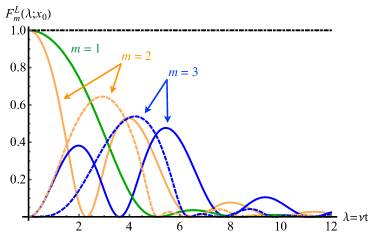
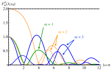
In Fig.1 we show the evolution of $F_{m}^{L}(\lambda;x_{0})$ as a function of $\lambda$ for three different values of the measured site $m=1,2,3$ and two different initial conditions: $x_{0}=1$ [Fig. 1(a)] and $x_{0}=2$ [Fig. 1(b)]. At $t=0$ the Fisher information $F_{x_{0}}^{L}(\lambda;x_{0})$ of the observable $|x_{0}\rangle\langle x_{0}|$ saturates the quantum Fisher information; this is a general fact: given an arbitrary initial condition $|\psi_{0}\rangle=\delta_{x,x_{0}}|x\rangle$, the most efficient projective measurement is the projector $|x_{0}\rangle\langle x_{0}|$. The Fisher information $F_{m}^{L}(\lambda;x_{0})$, on the other hand, does not saturate the quantum Fisher information; its maximum, achieved after an interaction time proportional to $|m-x_{0}|/\nu$, is, in general, well below the quantum Fisher information threshold.

(a)   $x_{0}=1$

(b)   $x_{0}=2$

Figure 1: (Color online) Fisher information for the local measurement $F_{m}^{L}(\lambda;x_{0})$ (solid lines) and for the Feynman probe $F_{m}^{P}(\lambda;x_{0})$ (dashed lines) as a function of $\lambda=\nu t$. The data refer to a chain of $s=10$ spins for different values of the measured or plugging site: $m=1$ (green lines ), $m=2$ (orange lines), and $m=3$ (blue lines). (a) Initial condition set to $x_{0}=1$; (b) $x_{0}=2$. In both frames the dot-dashed black line represents the quantum Fisher information.

IV Feynman Probes

Feynman’s quantum computer feyn87 consists of two logically separated parts; one part, the clock, is an excitation moving along a lattice. The second part, the input-output register, is a collection of additional degrees of freedom, say $n$ spin-1/2 particles $\vec{\sigma}^{j}$, $j=1,2,\ldots,n$. The overall system is governed by the time-independent Hamiltonian:

$${\cal H}_{F}=-\frac{\nu}{2}\sum_{j=1}^{s-1}|j+1\rangle\langle j|\otimes U_{j}+|j\rangle\langle j+1|\otimes U_{j}^{-1}.$$ (26)

Each term of the Hamiltonian involves two nearest neighbor sites of the clock and a self-adjoint or unitary operator $U_{j}$ acting on the register. The ordered product $U_{s-1}\ldots U_{2}U_{1}$ realizes some input-output transformation that the computing device is expected to accomplish. Figure 2 shows the architecture of the machine.

Figure 2: A schematic representation of the Feynman quantum computer

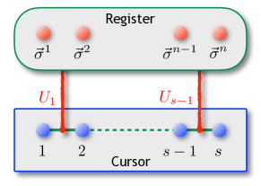
Because of the properties of the Hamiltonian ${\cal H}_{F}$, the position of the excitation in the clock, i.e., along the chain, uniquely determines the state of the register. This fact has interesting consequences. Let us consider the overall machine initially prepared in the state $|\psi_{0}\rangle=|1\rangle\otimes|R_{1}\rangle\equiv|1,R(1)\rangle$, i.e., with the excitation located at the beginning of the chain and the register in the pure initial state $|R_{1}\rangle$. Then the set

$$\mathcal{B}(\psi_{0})=\{|1,R_{1}\rangle,|2,R_{2}\rangle,\ldots,|s,R_{s}\rangle\},$$

where $|R_{j}\rangle=U_{j-1}\ldots U_{2}U_{1}|R_{1}\rangle$, constitutes an orthonormal computational basis, often referred to as the Peres basis peres85 , for the region of the Hilbert space visited by the evolved state $|\psi_{t}\rangle=\exp(-i{\cal H}_{F}t)|\psi_{0}\rangle$. This basis may be defined constructively for any choice of the initial condition $|\psi_{0}\rangle$. We refer to the space spanned by the Peres basis as the computational subspace. In particular, if upon measurement the clock is found at the rightmost site of the chain, the register collapses to the output state $|R(s)\rangle=U_{s-1}\ldots U_{2}U_{1}|R(1)\rangle$. Before discussing the kinematics of the clock, we point out that the sole effect of the interaction of the clock with the register of $n$ spins is the appearance of a degeneracy of order $2^{n}$ in the spectrum $\{e_{k}(\nu)\}_{k=1}^{s}$ of the tight-binding (clock) Hamiltonian

$${\cal H}_{0}=-\frac{\nu}{2}\sum_{j=1}^{s-1}|j+1\rangle\langle j|+|j\rangle\langle j+1|,$$

i.e. the Hamiltonian (3). Once an initial condition of the form $|\psi_{0}\rangle=|1,R(1)\rangle$ has been set, however, the spectrum of the Hamiltonian ${\cal H}_{F}$, restricted to the computational subspace, is no longer degenerate. In this subspace, the eigenvector

$$|v_{k}\rangle =\sqrt{\frac{2}{s+1}}\sum_{j=1}^{s}\sin\left(\frac{k\pi j}{s+1}\right)|j,R(j)\rangle.$$ (27)

corresponds to each eigenvalue $e_{k}(\nu)$. The properties of the Feynman quantum computer have been extensively discussed def06 ; def13 . The most relevant property of the Feynman machine that we want to exploit here is the entanglement between the clock and the register. The idea is to gain information about some physical parameter characterizing the clock by performing suitable measurements on the register alone. To this aim, we consider a streamlined version of the Feynman machine. Indeed, we consider a register made up of a single two-level system, which we refer to as the probe. The probe is initialized, without loss of generality, into the eigenstate of $\sigma_{z}$ belonging to the eigenvalue $+1$, or the up state $|\uparrow\rangle$. All the operators $U_{j}$ but the $m$-th one, $1\leq m\leq s-1$, are set to $\mathbb{I}$, whereas $U_{m}=\sigma_{x}$. In this setting, the Feynman Hamiltonian (26) reads

$${\cal H}_{F}(m) =-\frac{\nu}{2}\sum_{\begin{subarray}{c}j=1\\ j\neq m\end{subarray}}^{s-1}|j+1\rangle\langle j|+|j\rangle\langle j+1|+$$

$$-\frac{\nu}{2}\left(|m+1\rangle\langle m|\otimes\sigma_{x}+|m\rangle\langle m+1|\otimes\sigma_{x}\right).$$ (28)

If the clock is initially at a site $x_{0}\leq m$, the Peres basis for the system is

$$|1,\uparrow\rangle,\ldots,|m,\uparrow\rangle,|m+1,\downarrow\rangle,\ldots,|s,\downarrow\rangle.$$ (29)

Upon a projective measurement $\mathbb{I}\otimes|\uparrow\rangle\langle\uparrow|$ of the $\sigma_{z}$ component of the probe, the evolved state $|\psi_{\lambda}\rangle$ collapses into a state with support in either the $\operatorname{span}\left({|1,\uparrow\rangle,\ldots,|m,\uparrow\rangle}\right)$ or $\operatorname{span}\left(|m+1,\downarrow\rangle,\ldots,|s,\downarrow\rangle\right)$ subspace of the Hilbert space of states.

As a matter of fact, the Feynman structure provides a nonlocal alternative to characterize the qubit chain. Instead of measuring whether the excitation has left its initial position $x_{0}$, or reached a target one $x_{m}$, we can measure the $\sigma_{z}$ observable of the probe qubit, which we will now refer to as the Feynman probe. The Fisher information associated with such measurement is given by

$$F_{m}^{P}(\lambda;x_{0})=\frac{\left[\partial_{\lambda}P_{\lambda}(\uparrow|m,x_{0})\right]^{2}}{P_{\lambda}(\uparrow|m,x_{0})[1-P_{\lambda}(\uparrow|m,x_{0})]}$$ (30)

where

$$P_{\lambda}(\uparrow|m,x_{0})=|\langle\psi_{\lambda}|\uparrow\rangle|^{2}$$ (31)

is the probability of measuring the Feynman probe in the state $|\uparrow\rangle$, when it is plugged into the $m$-th site of the chain and the excitation is initially located at site $x_{0}$. Because of the probe-system entanglement, we have

$$P_{\lambda}(\uparrow|m,x_{0})=\sum_{x=1}^{m}|\langle\psi_{\lambda}|x\rangle|^{2}.$$ (32)

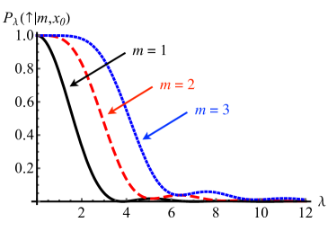
The behavior of $F_{m}^{P}(\lambda;x_{0})$ for three different plugging sites $m=1,2,3$ and two different initial positions $x_{0}=1,2$ is shown in Fig.1. For $x_{0}=1$ and $m=1$ a Feynman probe provides the same information as a local measurement, i.e. $F_{1}^{L}(\lambda;1)=F_{1}^{P}(\lambda;1)$. For $m=2$, $F_{2}^{L}(\lambda;1)$ still saturates the quantum Fisher information at $t=0$, whereas $F_{2}^{P}(\lambda;1)$ does not. For $m\geq 3$, the maximum Fisher information for the Feynman probe is typically larger than the Fisher information of the corresponding local measurement, whereas for $x_{0}>1$, local measurements typically carry more information than the Feynman probe for any value of $m>1$.

Overall, from the point of view of the efficiency of the measurement scheme alone, our results show that the ultimate bounds to the precision of Feynman probes are enhanced compared to those of local measurements when the excitation is initially located at the boundary of the chain and $m>2$. On the other hand, a proper comparison should be made in terms of an actual estimation strategy and thas is the scope of the next section.

Notice that the implementation of the Feynman Hamiltonian of Eq. (28) involves a three-spin interaction. This may be challenging from the experimental point of view. On the other hand, promising proposals based on cold atoms in optical lattices have already been discussed duan03 ; plenio04 ; cosco16 .

Figure 3: (Color online) $P_{\lambda}^{L}(m|x_{0})$ (top plot) and $P_{\lambda}(\uparrow|m,x_{0})$ (bottom plot) as defined in Eqs. (25) and (31) respectively, as a function of the parameter $\lambda$. The excitation is initially localized in the first site $x_{0}=1$ of a chain of length $s=10$. Three different values of $m$ are considered: $m=1$, (solid black line), $m=2$ (dashed red line) and $m=3$ (blue dotted line).

V Bayesian estimation

Figure 4: (Color online) (Top) Success probability in a single trial for LM and FP as defined in Eqs. (25) and (31), respectively; (bottom) Bayesian probability $P_{B}(\lambda|\Omega)$ defined in Eq. (33). The plots refer to simulations of (left column) LM on the site $m=1$; (middle column) LM on the site $m=2$ and (right column) FP coupled to site $m=2$. In the bottom plots, we use the true values $\lambda_{T}=1$ (solid black line), $2$ (dashed red line) and $3$ (dotted green line). The vertical lines are a guide for the eye marking the values of $\lambda_{T}$.

Classical and quantum CR theorems pose bounds to the precision of any unbiased estimator of the parameter of interest. However, no recipes are given to find optimal estimators saturating the classical bound. Therefore, in order to properly compare the performances of the local measurement (LM) and of the Feynman probe (FP), and to assess them against the ultimate quantum bound, we employ a Bayesian estimation strategy for the parameter $\lambda$, starting from a numerically simulated set of experimental data. Indeed, Bayesian estimators are known to be asymptotically optimal; that is, they saturate the CR bound for large data samples. Hereafter, we fix the initial position of the excitation in the first site $|x_{0}\rangle=|1\rangle$. The key ingredient in the Bayesian estimation is the Bayes theorem, which we can rewrite as:

$$P_{B}(\lambda|\Omega)=\frac{P(\Omega|\lambda)P(\lambda)}{\int P(\Omega|\lambda^{\prime})P(\lambda^{\prime})d\lambda^{\prime}}$$ (33)

where $P_{B}(\lambda|\Omega)$ is the a posteriori Bayesian probability distribution of the parameter $\lambda$ given the set of experimental data $\Omega$, whereas $P(\lambda)$ is the a priori probability distribution of $\lambda$. We assume we do not have any prior knowledge about the estimable parameter, so we can consider a flat distribution for $P(\lambda)$. The quantity $P(\Omega|\lambda)$ is the likelihood of obtaining the set of experimental data $\Omega$ when the true value of the parameter is $\lambda$. In our case, we have $M$ identical repeated Bernoulli trials, each of which is characterized by a success probability $p_{\lambda}$, then the likelihood of having $N_{0}$ successes out of $M$ is given by

$$P(\Omega|\lambda)=p_{\lambda}^{N_{0}}\,\left(1-p_{\lambda}\right)^{M-N_{0}}.$$ (34)

If the performed measures are local measurements on a site $m$, then $p_{\lambda}=P^{L}_{\lambda}(m|x_{0})$, while in the case we measure the Feynman probe coupled to sites $m$ and $m+1$, we have $p_{\lambda}=P_{\lambda}(\uparrow|m,x_{0})$. Once we reconstruct the Bayesian probability distribution (33), we can estimate the parameter as the expectation of the random variable $\lambda$:

$$\hat{\lambda}=\int\,\lambda P_{B}(\lambda|\Omega)d\lambda.$$ (35)

Accordingly, the variance of such an estimator is computed as:

$$\sigma^{2}[\hat{\lambda}]=\int\,[\lambda-\hat{\lambda}]^{2}P_{B}(\lambda|\Omega)d\lambda.$$ (36)

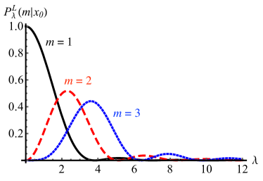
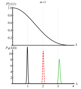
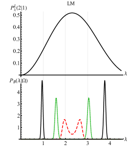
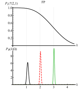
The probability $P_{\lambda}^{L}(m|x_{0})$ of measuring the excitation on site $m$ is shown in Fig. 3 for three different values of $m$, together with the probability $P_{\lambda}(\uparrow|m,x_{0})$ of measuring the FP in the state $|\uparrow\rangle$ when it is plugged between sites $m$ and $m+1$. If we perform a local measurement on the first site $m=1$, then $P_{\lambda}^{L}(1|1)=P_{\lambda}(\uparrow|1,1)$ and the two strategies are equivalent. The behavior of this probability is shown in Fig. 4. The success probability for each of the $M$ trials has a monotonic behavior, giving rise to a single-peak Bayesian probability distribution. The width of the peak is related to the variance of the estimator. If we measure any site other than the first one, then the local measurement and the FP strategy lead to dramatically different results, as shown in Fig. 4. We first notice that the probability $P_{\lambda}^{L}(m|1)$ is not invertible as a function of $\lambda$ except for the value corresponding to its maximum. On the other hand, it is possible to find a value $\lambda_{max}$ such that $P_{\lambda}(\uparrow|m,1)$ is invertible in the region $[0,\lambda_{\max}]$ of the parameter space. This has profound consequences on the reliability of the two estimation procedure, because it affects the shape of the a posteriori probability distribution for estimating the parameter. In fact, the Bayesian probability built according to Eq. (33) has two peaks for a local measurement procedure, corresponding to the two values of the parameter $\lambda$ which give the same probability $P_{\lambda}^{L}(m|x_{0})$, and a single maximum for the FP estimator. Indeed, the probability distribution $P_{\lambda}^{L}(m|x_{0})$ is non-monotonic, showing a maximum corresponding to the only value of the parameter $\lambda$ that can be estimated without any prior knowledge about $\lambda_{T}$. For any other values of $\lambda_{T}$, the local measurement strategy fails to uniquely identify a single solution for the estimation procedure and a two-peak probability distribution $P_{B}(\lambda|\Omega)$ is obtained. For $\lambda_{T}$ approaching the maximum of the distribution, the two peaks start to merge, leading to a broad probability distribution. On the contrary, the FP success probability keeps its monotonic behavior in the whole parameter region and thus Bayesian inversion strategy always leads to a single solution, within the variance of the estimator. Except for the case where the local measurement is performed on the first node $|1\rangle$ of the lattice, a presence measurement on any other site will give a a-posteriori probability distribution with two peaks, i.e. the Bayesian estimation procedure identifies two possible solutions $\lambda_{1}$, $\lambda_{2}$. Since there is no way to discriminate between $\lambda_{1}$ and $\lambda_{2}$ without any a-priori knowledge, the local measurement cannot provide a reliable estimation of the coupling strength $\nu=\frac{\lambda}{t}$. Measuring the state of the FP, on the other hand, allows us to correctly infer the value of $\lambda$, within an error given by the width of the single-peak reconstructed Bayesian probability distribution. Once we fix the time at which we perform the measurement $t_{M}$, the coupling constant is easily identified as $\nu=\lambda/t_{M}$.

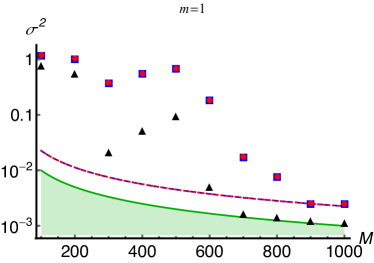
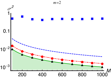
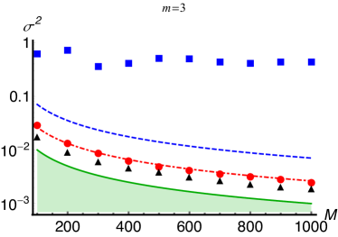
The Bayesian FP estimator saturates the CR bound (7), as shown in Fig. 5. However, as we have already mentioned, neither the LM nor the FP allows us to saturate the quantum CR bound. In order to improve precision we may use a two-step scheme, in which we first employ the Feynman probe and Bayesian estimation and then use the posterior distribution for $\lambda$ as a prior for Bayesian estimation using local measurements. This procedure allows us to build a more precise estimator, with a smaller variance compared to those obtained using solely local measurements or Feynman probes. The variance $\sigma^{2}$ obtained from a set of $M$ simulated experiments which employ this LM+FP scheme is shown in Fig. (5) (black dots). As it is apparent from the plot the two-step scheme performs better than the other measurements schemes and it allows one to achieve, in some cases, the quantum CR bound, thus representing an optimal procedure to characterize linear chain of qubits.

Figure 5: (Color online) Variance for the LM (blue squares), FP (red circles) and combined FP+LM (black triangles) estimators as a function of the number $M$ of repeated simulated measurements, for $\lambda_{T}=3$. Each plot refers to a different value of the measured (or plugging) site $m$. The blue dashed line and the red dot-dashed one highlight the limit imposed by the CR bound for LM and FP measurements respectively. The green shaded area delimits the region forbidden by the quantum CR bound.

VI Conclusion and outlook

In this paper we have introduced a novel estimation procedure based on Feynman probes for the characterization of linear qubit chains made of strongly interacting two-level systems. A Feynman probe is a single-qubit register coupled to the chain of qubits, which is initially prepared in a single-excitation state. The probe is dynamically entangled to the excitation moving along the linear chain and by measuring the state of the probe it is possible to extract information on the value of the coupling constant.

First, we evaluated the quantum Fisher information associated with the coupling parameter, thus determining the ultimate precision of any estimation procedure. We then showed that local measurements, i.e. measuring the presence of the excitation on a single site, provide optimal characterization of $\lambda$ for small values of the coupling. In particular, optimal estimation is obtained when the local measurement is performed at site $x_{0}$, where the excitation is initially localized. In this regime the CR bound may be attained by Bayesian estimation, for a large number of repeated measurements. On the contrary, for larger values of the coupling $\lambda$, i.e. for strongly coupled chains of qubits, a Bayesian local strategy does not lead to a consistent estimate, because the a-posteriori probability distribution shows two peaks. In this regime, Feynman probes provide a consistent Bayesian estimator that saturates the CR bound, i.e. it achieves efficient characterization of the qubit system. We concluded that characterization by Feynman probes represents a suitable estimation strategy for a strongly coupled qubit chain.

Finally, we suggested a two-step measurement scheme where both FP and LM are employed one after the other to estimate the coupling $\lambda$. In the first step, FP is used to infer the coupling: the resulting distribution is then used as an a-priori distribution for a Bayesian LM estimation $\lambda$. The overall precision may achieve the quantum CR bound. Our results provide an alternative route to characterize qubit systems and confirm the relevance of nonlocal measurements, which have already been suggested as a convenient toolbox for quantum circuits based on trapped ions ti1 ; ti2 and supeconducting qubits nig13 ; blu16 . Feynman probes could also be employed to estimate the current in out of equilibrium quantum wires benenti09 ; clark13 or the amount of disorder in linear lattices lahini08 ; tama09 .

As we pointed out, cold atoms in optical lattices are promising systems for the realization of the three-spin interaction needed by Feynman probes. Our results confirm the interest of these systems and may foster future research about an implementation of the Feynman probe mechanism based on current quantum technology. This would allow us also to extend our analysis addressing the robustness of the Feynman probe estimation procedure against experimental imperfections.