SMU-HEP-16-06
Reconstruction of Monte Carlo replicas from Hessian parton distributions
Abstract
We explore connections between two common methods for quantifying the uncertainty in parton distribution functions (PDFs), based on the Hessian error matrix and Monte-Carlo sampling. CT14 parton distributions in the Hessian representation are converted into Monte-Carlo replicas by a numerical method that reproduces important properties of CT14 Hessian PDFs: the asymmetry of CT14 uncertainties and positivity of individual parton distributions. The ensembles of CT14 Monte-Carlo replicas constructed this way at NNLO and NLO are suitable for various collider applications, such as cross section reweighting. Master formulas for computation of asymmetric standard deviations in the Monte-Carlo representation are derived. A correction is proposed to address a bias in asymmetric uncertainties introduced by the Taylor series approximation. A numerical program is made available for conversion of Hessian PDFs into Monte-Carlo replicas according to normal, log-normal, and Watt-Thorne sampling procedures.
pacs:
12.15.Ji, 12.38 Cy, 13.85.QkI Introduction
Modern parton distribution functions (PDFs) Dulat et al. (2016); Harland-Lang et al. (2015); Ball et al. (2015); Abramowicz et al. (2015); Alekhin et al. (2014); Accardi et al. (2016) are provided with estimates of uncertainties from multiple origins. These estimates are essential for understanding of the accuracy of collider predictions, both for precision measurements and for new physics searches. PDFs are determined from a global statistical analysis of diverse experimental measurements, in deep-inelastic scattering, in production of vector bosons and jets, and in other hard-scattering processes. An optimal parametrization of the PDFs is obtained by a minimization of the figure-of-merit function () that quantifies the level of agreement between experimental data and theoretical predictions. The minimization is performed with respect to the PDF parameters of interest, and with respect to nuisance parameters associated with theory, experiment and the data analysis procedure. Once the best-fit PDF parametrization is found, additional parametrizations are constructed for estimating the total PDF uncertainty. In this paper, we explore the connection between two methods for quantifying PDF uncertainties, one based on the diagonalization of the Hessian error matrix Pumplin et al. (2001), and one on the stochastic (Monte-Carlo) sampling of parton distributions Giele and Keller (1998); Giele et al. (2001). PDF uncertainties can also be determined by the Lagrange multiplier Stump et al. (2001) and offset Cooper-Sarkar (2002) methods, but the PDFs obtained with the Hessian and Monte-Carlo techniques are the most commonly used.
In any method of PDF error analysis, the ultimate goal is to provide information about the probability distribution in the space of PDF parameter values. This information can be presented in several forms. Much of PDF research Dulat et al. (2016); Alekhin et al. (2014); Abramowicz et al. (2015); Harland-Lang et al. (2015); Accardi et al. (2016) relies on an analytic minimization on a class of PDF parametrization forms, in the same manner as in the CT global analyses. Since can be approximated by a quadratic function of PDF parameters in the neighborhood of the global minimum, a boundary of the hyperellipsoid containing a specified cumulative probability can be delineated with a relatively small number of error PDFs, corresponding to the eigenvectors of the Hessian matrix. The PDF uncertainty on a QCD observable , at a confidence level , is derived via algebraic “master formulas” Pumplin et al. (2001, 2002) from values for calculated for each eigenvector set . In the Gaussian approximation, the PDF errors on in the positive and negative directions are equal. If deviations from the Gaussian behavior are mild, then the asymmetry between the positive and negative PDF errors can be estimated in the Hessian approach, too, using master formulas requiring two error sets per each eigenvector direction Nadolsky and Sullivan (2001).
An alternative NNPDF Monte-Carlo technique Forte et al. (2002); Del Debbio et al. (2007); Ball et al. (2009, 2013, 2015) provides an ensemble of error PDF sets, or “replicas”, which sample the functional forms of parton distributions parametrized by neural networks, with little bias due to the choice of the parametrization form. The probability distribution in the hypervolume can in principle be fully reconstructed, given a sufficiently large ensemble of PDF replicas. The prediction for a QCD observable is then obtained from the mean and standard deviation of the values of for each member of the (large) Monte-Carlo replica ensemble.
Hessian eigenvector sets can be converted into Monte Carlo replicas Watt and Thorne (2012), and vice versa Gao and Nadolsky (2014); Carrazza et al. (2015a); Carrazza et al. (2016). Small Hessian eigenvector ensembles are sufficient, and desirable, for many applications. Monte Carlo calculations based on a large ensemble of replica PDFs allow the implementation of new experimental constraints on the PDFs using replica re-weighting Giele and Keller (1998); Ball et al. (2011, 2012). The full ensemble of Monte Carlo replicas can be recast into an ensemble with fewer replicas by unweighting Ball et al. (2012), by compression Carrazza et al. (2015b), or by conversion into a Hessian ensemble Gao and Nadolsky (2014); Carrazza et al. (2015a); Carrazza et al. (2016), while retaining the core statistical information. PDF ensembles from several groups can be combined by converting the Hessian ensembles into a Monte-Carlo representation, and then reducing/compressing the combined MC ensemble into a smaller Hessian or MC ensemble. These techniques are employed to combine the error PDFs from CT14, MMHT’14, and NNPDF3.0 into smaller PDF4LHC15 ensembles according to the recommendation of the PDF4LHC Working Group Butterworth et al. (2016).
Conversion of the Hessian eigenvector sets into Monte-Carlo replica sets is employed in several such applications and influences the outcomes for the uncertainties and even central predictions. The PDF conversion must be understood in order to trust this method. The Watt-Thorne prescription Watt and Thorne (2012) provides the simplest realization of the conversion method, under the approximations of the exactly Gaussian distribution of the PDF parameters and linear dependence of error PDFs on small variations of the PDF parameters. It is desirable, however, to develop a formalism that can go beyond the linear approximation and, given enough Hessian sets, reproduce non-linear features of the probability distribution such as asymmetry.
This paper lays out such general formalism. It allows one to systematically include nonlinear PDF dependence and may produce different outcomes in some LHC predictions compared to the Watt-Thorne method, as we will demonstrate. To apply the general conversion method, we first construct Monte-Carlo replica ensembles that reproduce both the symmetric and asymmetric uncertainties of the CT14 Hessian sets, and also generate positive-definite replica parametrizations if desired. The resulting PDF uncertainties with MC replicas are closer to CT14 asymmetric uncertainties, compared to the Watt-Thorne method. Reconstruction of the full probability distribution from the Hessian sets reveals several subtleties, see Sec. IIB. In particular, naive Monte-Carlo sampling of the PDFs using the Taylor series results in biased asymmetric uncertainty bands that can be corrected.
It is also instructive to compare statistical properties of the CT14 MC replica ensemble (obtained by conversion) and NNPDF MC replica ensemble (obtained using a genetic algorithm). Despite drastic differences in the two replica generation methods, we demonstrate in Sec. IIIB that the statistical properties of two MC replica ensembles have deep similarities, and explain why.
In Sec. II we compare formulas for the estimation of Hessian and MC uncertainties and derive prescriptions for the generation of MC replicas that generalize the Watt-Thorne prescription. These prescriptions account for asymmetry of PDF errors in the same manner as in the CT14 Hessian set. At the end of the section, we show how to construct individual replica sets that reproduce the positivity requirement imposed on the CT14 Hessian sets. Sec. III compares PDFs, parton luminosities, predictions for LHC cross sections, and their uncertainties obtained with the CT14 Hessian and MC PDFs. In Sec. III.2 we examine statistical properties of the replica ensemble, and consider the agreement of individual replicas with the experiments in the global fit. Sec. IV contains concluding remarks and information on the availability of the CT14 replica PDFs. A computer program is presented for generation of MC replicas according to the new prescriptions that optimally reproduce the Hessian uncertainties and positivity.
II Generation of Monte-Carlo replicas from Hessian error PDFs
II.1 Master formulas for Hessian PDFs
The CT14 parton distribution functions (PDFs) were generated in a global analysis of QCD, by fitting theoretical calculations, at LO, NLO and NNLO, to experimental data for a wide variety of high- processes Dulat et al. (2016). Once the central (most probable) combination of PDF parameters is found by minimization of the log-likelihood function , special “error PDF sets” are constructed to characterize and propagate PDF uncertainties. The error PDFs do not specify all features of the probability distribution in the fit, only a part needed for estimating uncertainties in typical applications. In the Hessian method used by CTEQ, the error PDFs, called “eigenvector sets”, keep information about the first and second moments of the probability distribution, sufficient for estimation of central values, standard deviations, and PDF-driven correlations. A PDF ensemble based on MC replicas, when obtained directly from the fit, can in principle reproduce the primordial probability distribution with better accuracy; in practice, its size is commonly limited to no more than a thousand replicas, also enough for reproducing up to the second moments.
Therefore, the error sets primarily quantify the lowest two moments of the primordial probability; and a Hessian eigenvector set is often the only published output from the PDF fit. For the applications utilizing MC replicas, especially when large numbers of replicas are to be generated on the fly, one may wish to convert the Hessian PDF ensemble into an MC replica one, according to the procedure that will be laid out. [A computer code implementing this procedure is available for downloading.] The converted MC replicas must ideally preserve the statistical features of the Hessian ensemble. They cannot provide more information about the primordial higher moments than what is available in the Hessian ensemble.
Let us focus for a moment on the construction and properties of the CT Hessian sets. The PDFs are parametrized at by a functional form which depends on a set of adjustable parameters, . A test statistic is defined as in Lai et al. (2010); Gao et al. (2014) to measure the difference between theory and data. Its explicit definition is reproduced in the appendix. The minimum of defines the central fit, and the variation of in a neighborhood of the minimum provides the uncertainty in the fit. Thus, the approximation in the vicinity of the minimum,
| (1) |
has two parts. First, the central combination of the parameters, which corresponds, without loss of generality, to all zero values (, gives the “best” fit between theory and data, for which is minimized: Second, the approximately quadratic behavior of very close to the minimum allows one to define independent directions in space, corresponding to eigenvectors of the Hessian matrix The eigenvectors are used to determine the uncertainty on PDFs and on any quantities that depend on them, by computing variations of along each independent direction Pumplin et al. (2001).
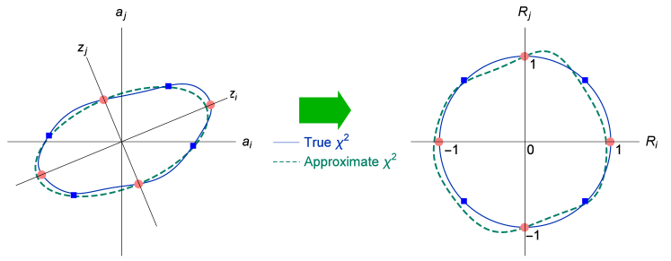
In this scheme, the independent directions are determined by relying on the quadratic approximation for ; at the same time, extreme displacements along each eigenvector direction are found from variations of the true (not perfectly quadratic) This is illustrated in the left inset of Fig. 1, showing contours of constant values of the exact and approximate for a certain pair of parameters, . The minimum of the exact is reached at the axes origin; the solid and dashed contours are drawn for constant increases of with respect to the minima of the exact and its quadratic approximation. The directions are along the axes of the approximate ellipsoid. The extreme displacements are found by demanding the increase in the true, not approximate, . They correspond to the (filled) red circles at the intersections of the axes and the irregular contours of the true in the left-hand side of Fig. 1. Note that both the functional form of the true and the value of depend on the context of the analysis. In CT fits Lai et al. (2010); Gao et al. (2014), the true that determines the uncertainties consists of two tiers of conditions, quantifying the global agreement with the experiments, and deviations from individual experiments, cf. the appendix. The parameter is set to 10 at 90% confidence level (c.l.). The complex nature of true implies that, most generally, ; still, its overall features are captured well by the approximate quadratic .
This introduces one source of asymmetry in PDF errors, due to the cubic and higher sign-odd powers of in the full . The impact of this source is reduced by rescaling of the parameters to satisfy Keep in mind that disagreements of the primordial -dependent probability with the Gaussian behavior are weak to start with, and that the Hessian sets specify the probability (i.e., ) only at three points per an eigenvector direction. Aside from the above conditions at the three points, we will not need to know the rescaling function in the rest of the discussion.111An example of the rescaling function for one eigenvector direction is a steplike one, . The parameter controls the smoothness of the step transition, it is at least as small as . Far enough from , the step function reduces to and , for positive and negative , respectively. The probability distribution in terms of is even closer to the Gaussian one:
| (2) |
The transformation is illustrated by the right-hand side of Fig. 1. This approximation is known from experience to hold well in CT fits within the 90% c.l. region around the best fit, even though large (greater than 1.5) may be excluded by tier-2 penalties on that enforce agreement with the individual fitted experiments Lai et al. (2010); Gao et al. (2014).
Next, we consider a function of the parameters , such as the PDF or even the QCD cross section. This function may have asymmetric uncertainties, regardless of symmetry of . Expanding near the global minimum in the Taylor series up to the second derivatives, we have
| (3) |
The derivatives can be estimated by finite differences,
| (4) | |||||
| (5) | |||||
| (6) |
In these equations, the values are taken at the global minimum,
| (7) |
at the red circles on the axes in Fig. 1,
| (8) |
and at the blue squares on the diagonals,
| (9) |
We see that the Hessian eigenvector sets corresponding to are sufficient for computing the first and diagonal second derivatives, and . The mixed second derivatives would require additional error sets for . Those off-diagonal error sets are not provided in the conventional PDF analyses.
The Taylor expansion of can be used to construct various master formulas for the estimation of Hessian PDF uncertainties. Keeping only linear terms on the right-hand side of Eq. (3), one obtains
| (10) |
If are reached at the boundary of the 68% c.l. region (and the Hessian eigenvector sets are determined according to this convention), the maximal variation of within the unit hypersphere of
| (11) |
yields the Hessian symmetric PDF uncertainty at 68% c.l., denoted by Pumplin et al. (2001). However, the published CT14 parametrizations correspond to the 90% c.l. Using the same master formula, we find the 90% c.l. uncertainty from the CT14 sets, satisfying .
If the diagonal second-order derivatives are also included, Eqs. (10) and (11) are modified to
| (12) |
Also, asymmetric uncertainties on can be estimated by Nadolsky and Sullivan (2001)
| (13) | |||||
| (14) |
The absolute values of the asymmetric uncertainties are generally not the same for the positive () and negative () displacements Nadolsky and Sullivan (2001). For example, and must have opposite signs if varies linearly with , but they can have the same sign if the nonlinearity of is large and hence result in a zero contribution to either or . In the CT convention, low-number eigenvectors, corresponding to the best-determined directions, tend to be more symmetric (with opposite-sign variations), while high-number eigenvectors can be strongly asymmetric.
II.2 Probability density distribution for
We will now formulate a set of requirements for Monte-Carlo replica generation that will be applied in the next subsection to devise our replica generation method. A reader interested in the specific formulas for replica generation may skip this subsection and proceed to the next.
The Monte-Carlo replicas quantify the full probability density distribution for a QCD observable , going beyond the intervals of fixed probability available with the Hessian PDFs. A priori, . The probability might be extracted directly from the fit by using a Lagrange multiplier scan or stochastic sampling of the exact log-likelihood . But, more often than not, the outcomes of the fit are initially stored in the form of the Hessian PDFs . The complete functional forms for the PDFs may be unavailable or difficult to sample. Then, one relies on constructing the Monte-Carlo replicas from the Taylor series for the Hessian PDF values provided in space, and without invoking the exact parametrization form.
In addition to the central prediction , the Hessian PDFs specify two values of per each eigenvector direction, that is, . This information is generally insufficient for reconstructing the true by Monte-Carlo sampling. Even the confidence of probability intervals for may remain undetermined!
Recall that, by their construction and using the parameter distribution , the 68% c.l. Hessian values correspond to the cumulative probabilities of about 16%, 50%, and 84%. When one naively samples assuming a multi-Gaussian distribution for one is not guaranteed to obtain the same cumulative probabilities for from the distribution of Monte-Carlo replicas, because of probability folding. When folding occurs, the 68% probability interval of the Monte-Carlo replica set distributed according to deviates from the 68% c.l. Hessian uncertainty interval found using . In the Gaussian case, the central combination of the PDF parameters, associated with the central CT14 PDF, is located at the mode, median, and mean of , as those coincide. On the other hand, the central CT14 prediction for does not automatically correspond to either the mode, median, or mean of which can be different.
Indeed, when is not monotonic, several combinations may produce the same value of Replicas of such obey a folded probability , meaning that the cumulative probability for getting is not equal to that for the corresponding . In the one-dimensional case, a simple example is with a normally distributed on . Then obeys a half-normal distribution on ; corresponds to the cumulative probabilities of 50% and 0% according to and , respectively.
If depends on one eigenvector parameter and is continuous and monotonic in intervals ,…, , then is invertible in each interval: for . We indicate that lies within using a notation with equal to or 0 if the statement is true or false, respectively.
The function is generally not normally distributed, even when is. That is, while
| (15) |
the probability density distribution does not need to be Gaussian. It satisfies
| (16) |
as follows from the normalization conditions for the probability densities,
| (17) |
Going back to the truncated Taylor series with a non-negligible ,
| (18) |
where the derivatives are estimated by the finite differences from and , we could solve for and find up to two solutions for per each value. [ is then given by Eq. (16) with .] Such truncated Taylor approximation is clearly not monotonic. We expect it to deviate from the true when the displacements are large, and to produce a folded probability distribution with a displaced median value and confidence intervals, as compared to the true . We may even end up with a problematic arrangement when the central CT14 Hessian prediction is outside of the nominal 68% probability interval of the replicas. These observations continue to hold when has components.
On the other hand, in a variety of important applications, our group observed that the Lagrange multiplier and Hessian methods render similar probability intervals. Most recently, the two methods were shown to predict compatible 68% and 90% confidence intervals for the common LHC observables, such as jet, Higgs, and production cross sections Dulat et al. (2016); Belyaev et al. (2006); Dulat et al. (2014a); Schmidt et al. (2014); Pumplin et al. (2009). This indicates that the impact of the second derivatives is mild in constrained regions, credible estimates for can be found via the sampling of the Hessian PDFs after correcting for the Taylor series’ imperfections. At intermediate where the nonlinearities in the PDF uncertainties are weak, the Taylor expansion performs well. The discrepancies are more pronounced at small and large Bjorken with fewer experimental constraints. Nonlinearities and folding effects are small for well-constrained eigenvector parameters and can be substantial for poorly constrained ones.
With these observations in mind, we design a Monte-Carlo sampling procedure for the PDFs using the Taylor series in the case of mild nonlinearities. First, rather than always sampling the PDFs , we may sample a function of of that reduces the impact of . For example, at moderate one could just sample the PDFs directly, i.e., set with normally distributed . At large where , Gaussian sampling of may be more desirable for suppressing the nonlinearities; we will show that the log-normal sampling leads to more physical behavior. We explore this possibility when generating positive-definite PDF replicas in Sec. II.4.
Second, we need to assign cumulative probabilities to the input values. Within the accuracy of the Hessian approximation, we can make use of the knowledge that the Hessian central value and Hessian uncertainties are close to the median and 68% central probability intervals for the PDFs, respectively. This “obvious” conclusion from the Lagrange Multiplier studies can be violated by naive sampling, hence we enforce it as a separate requirement. Furthermore, for mildly asymmetric populations, the median, with the cumulative probability of 0.5, tends to lie close to the mean given by the standard formula Kenney and Keeping (1954). In the various sampling scenarios that we had tried, we confirmed that the median of a PDF replica distribution differed little from the mean, except for in the extreme regions. It suffices to assume that the central Hessian PDF coincides with the mean of the PDF replica ensemble, easily computable from the replicas’ values and close to the median value. When the replica ensemble is first generated, the median/mean at each and may disagree from the central CT14 PDF as a consequence of the probability folding caused by the Taylor expansion, as well as because of residual fluctuations. We correct for this mismatch by a uniform shift in all PDF replica values, as explicated in the next section.
In Sec. III, we show that this sampling procedure reproduces the central CT14 Hessian prediction (coinciding with the mean of the MC replicas by construction), and the 68% probability intervals of the MC replicas approximate both the Hessian symmetric and asymmetric uncertainties.
II.3 Generation of Monte-Carlo replicas
We will now present the formulas to generate the Monte-Carlo PDF replicas. We produce sets of the PDF parameters, , which are randomly distributed according to the probability density . We will again rely on the experience that is typically close to the standard normal distribution, as in Eq. (2), with the mean (or, central) values corresponding to the best-fit PDF set, and the standard deviations that are found from the Hessian PDFs. Therefore the replicas will be sampled from the standard normal distribution in Eq. (2).
The Monte-Carlo replica of a QCD observable, , will be constructed as
| (19) |
in terms of the value for the central Hessian set, a random shift , and a constant shift applied to all replicas (. Examples of include the PDF, parton luminosity, cross section, or the logarithm of PDF discussed below. The parameter can be set to zero, as in the original Watt-Thorne method. But as was argued in Sec. II.2, we find it helpful to allow a shift of all replica values by a constant amount .
When is a PDF, we expect that within the accuracy of the Hessian approximation. [This relation does not hold for an arbitrary .] Monte-Carlo sampling of the Taylor series may disagree with this condition. The Taylor expansion may lead to systematic biases, as discussed above. That is, may differ from the mean over the replica ensemble,
| (20) |
even when is large. The mean also fluctuates around , as the number of replicas changes, but these fluctuations are small when is above a few hundred. If our goal is to reproduce the Hessian central value (“truth”) and Hessian uncertainties as closely as possible, we may correct such small offsets of the mean, after all are computed, by shifting all replicas by a constant amount
| (21) |
We then get , up to a small numerical uncertainty, when the replicas are generated according to Eqs. (19) and (21). This choice will be adopted as the default. The random displacements are found using Eq. (3), where for the -th replica. For the PDFs, , this prescription preserves the usual sum rules obeyed by the PDFs, since each replica is a linear combination of the Hessian eigenvector sets, which satisfy the sum rules individually.
Symmetric MC replicas. If only the first derivatives are retained in the Taylor series, then we have
| (22) |
On average, are symmetrically distributed in the positive and negative directions. The mean of the replicas, remains close to the central Hessian value with good accuracy, and the global shift can be neglected. The MC uncertainty on is then quantified by a standard deviation,
| (23) |
It is expected to approach the 68% c.l. symmetric Hessian uncertainty in Eq. (11), in the limit.
Asymmetric MC replicas. In analogy to Eq. (12) for the Hessian uncertainties, the diagonal second derivatives can be included as
| (24) |
In this case Eq. (19) must include the shift term to satisfy . Now the asymmetric error estimators are given by the standard deviations that include only positive (negative) displacements from the mean value:
| (25) | |||||
| (26) |
These are the MC counterparts of the asymmetric Hessian uncertainties, provided by Eqs. (13) and (14).
Compared to the previous work on the MC replicas, our prescription thus includes several new features: the generation of MC replicas using asymmetric displacements (24) derived from the Taylor series, a constant shift to ensure agreement between the central Hessian set and the mean of the replicas, and asymmetric standard deviations . Watt and Thorne Watt and Thorne (2012) provided the same formulas (22, 23) for generating the symmetric MC replicas. Their prescription for generating MC replicas with asymmetric displacements is different from the Taylor-series displacements in (24) and is given by
| (27) |
with
We advocate using the asymmetric standard deviations (25) and (26) as estimators for 68% c.l. PDF uncertainties, as they are simple, numerically close to the Hessian asymmetric estimators, cf. the next section, and converge rapidly with the number of replicas.222An alternative estimator, given by the 68% probability interval centered on the mean value, requires sorting the values and is more susceptible to random fluctuations. Another estimator, given by the maximal displacements of in the 68% probability hypersphere for , has slow convergence. In terms of the relative significance, using with shifts, together with the asymmetric standard deviations, is most important for reproducing the asymmetric Hessian uncertainties. As a secondary effect, mild numerical differences were also noticed between the Taylor-series formula (24) and Watt-Thorne formula (27) for displacements .
II.4 Monte-Carlo replicas for CT14 parton distributions
The formulas derived in Sec. II.3 are applicable for generating MC replicas for the PDFs themselves, with an extra modification. We perform a truncated Taylor series expansion of at every point, assuming small deviations from the central value . In unconstrained regions, the linear expansion is not sufficient – in fact, it may lead to unphysical solutions such as negative cross sections. Parametrizations for Hessian distributions from the CT family satisfy positivity constraints, , and render non-negative physical cross sections. To realize the positivity of each MC replica, and eventually to better approximate the non-linear probability distribution, we construct the replicas by Gaussian sampling of , rather than by sampling directly.
The final distribution of CT14 MC replicas includes two families at NNLO in the QCD coupling strength, with 1000 replica sets each, as well as two counterpart families at NLO. Replicas of the first type (linear MC, or MC1) are generated assuming normally distributed linear displacements of PDFs, corresponding to Eqs. (19), (24)-(26), with Replicas of this type are very similar in spirit to Watt-Thorne replicas; in particular, they may violate positivity.
Replicas of the second type (log MC, or MC2) are generated by sampling of a Gaussian distribution for whose variance is estimated as , and the mean value is set to , where as above. For the PDFs , we obtain a log-normal distribution with . When the PDF error is small, the variance of the PDFs, becomes equal to the squared Hessian error, . Recall that, if obeys a normal distribution with the mean and variance , then the mean and variance of are and . Consequently the “log MC” replicas reproduce the Hessian PDF uncertainty in well-constrained regions and stay non-negative in the poorly constrained regions.
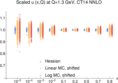
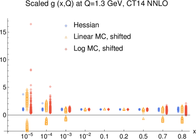
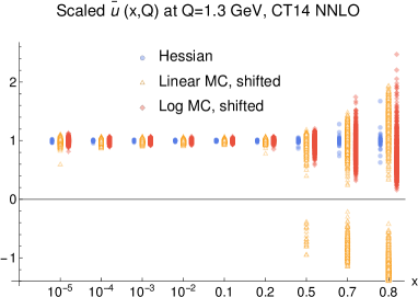
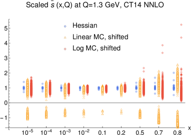
The difference between the two types of replicas is illustrated by Fig. 2, showing PDFs for the CT14 NNLO 56 Hessian eigenvector sets (blue circles) and 1000 MC replicas obtained with linear sampling (orange triangles) and logarithmic sampling (red diamonds). The MC replicas are shifted as described above to have equal to , the central PDF of the Hessian set. The vertical axis is scaled as to better visualize relative variations of both signs in an extended magnitude range.
The value of 1 corresponds to the replica PDF coinciding with that of the central set. The majority of replicas produce PDF values that are close to the central PDF set, within the intervals enclosing 1 where many replica symbols overlap. Some replicas for less constrained PDFs produce very large deviations, corresponding to the values far from 1. The Hessian and log-sampled replicas are non-negative by construction, facilitating positivity of physical cross sections. The linearly sampled replicas can take negative values in extrapolation regions (i.e., lie below the horizontal line at zero). In practice, it is desirable to have non-negative cross sections for individual replicas, even though the uncertainty band does extend to zero at some confidence level.
III Comparisons of replica sets and Hessian error PDFs
III.1 Estimation of PDF uncertainties
To justify the use of the replica sets for estimating the PDF uncertainties, we must first show that the mean and standard deviation of the replica PDFs themselves are consistent with the results obtained directly from the Hessian error PDFs. A complete set of the comparisons is available at CT1 (a). The PDFs are generated by sampling LHAPDF6 grid files using the mcgen code MCG .
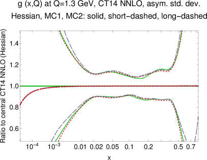
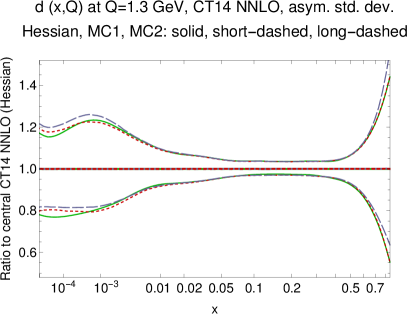
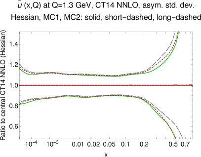
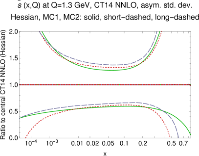
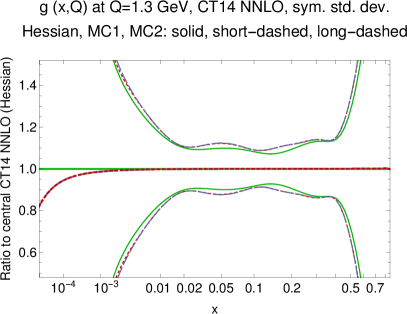
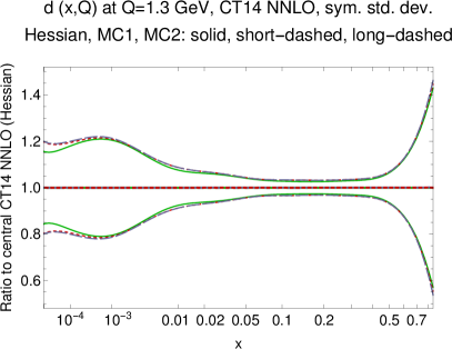
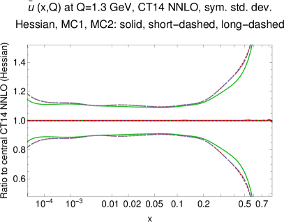
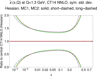
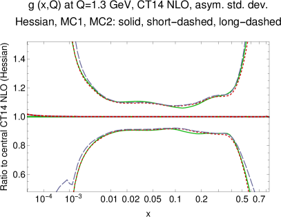
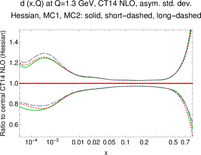
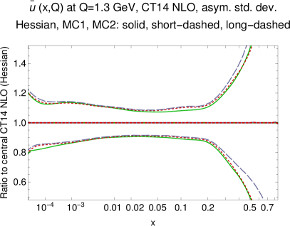
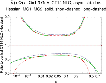
Figure 3 shows the values and error bands, for the ratios of , , and PDFs to the respective central CT14 PDFs, at the initial scale GeV, at NNLO. The three green solid curves represent the central PDF (for which the ratio is 1), and the asymmetric upward and downward 68% c.l. deviations calculated from the Hessian master formulae (13) and (14). The red short-dashed and blue long-dashed curves show the mean and the error bands corresponding to asymmetric standard deviations of the CT14 MC1 and MC2 ensembles with 1000 replicas. We see in the figure that the Hessian and replica PDFs are very consistent in terms of both the means and standard values.333The central gluon PDF from the replica set is slightly lower than the Hessian one in the upper left Fig. 3 at and GeV, where the CT14 gluon vanishes, as a result of numerical roundoff errors. Both MC1 and MC2 ensembles, obtained by linear and logarithmic sampling of the replicas, result in agreement of comparable quality with the Hessian PDFs at intermediate In the extreme regions, the MC2 error bands tend to be slightly shifted toward positive values. The differences may be somewhat more noticeable for the poorly constrained strangeness PDF, but in all cases the Hessian and MC error bands are fully compatible within the uncertainties of the definition of PDF errors.
In the case of symmetric Hessian uncertainties (11) and symmetric standard deviations (23), the agreement of Hessian, MC1, and MC2 NNLO ensembles is even better. The corresponding comparisons are shown in Fig. 4. Equivalent comparisons for CT14 NLO asymmetric errors are presented in Fig. 5. These figures compare the parton distribution functions at the initial momentum scale . If we evolve these to any using the DGLAP equations, the agreement between the three ensembles further improves. Figures with comparisons of the CT14 Hessian, MC1, and MC2 PDFs at and GeV can be viewed at CT1 (a).
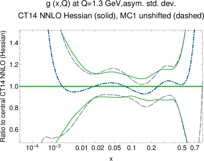
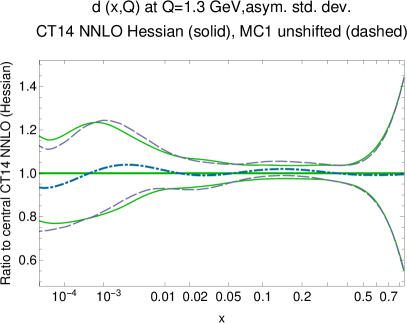
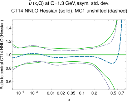
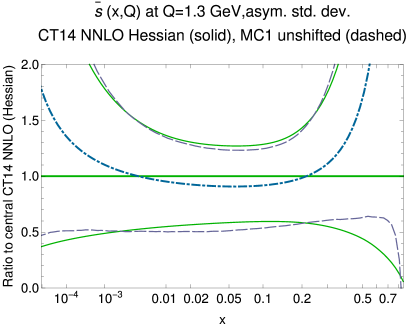
Lastly, in Fig. 6, we compare the CT14 NNLO Hessian PDFs to a MC1 version that does not shift the replicas by a constant amount . In this case, the whole bands are shifted compared to the Hessian band across all , by following their wiggly mean PDFs. [The reader can generate the unshifted replica ensemble with the mcgen program if desired.] As was argued in the previous section, the shift is introduced to eliminate such spurious variations introduced by truncation of the Taylor series.
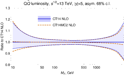
It is also useful to compare the luminosity functions and their uncertainties, for the MC replicas and the Hessian PDFs. The luminosity function of a parton-parton pair, for production of a final state at collider energy , is defined as in Campbell et al. (2007), with an additional constraint that the rapidity of the final state, given by , does not exceed in magnitude:
| (28) |
The gluon-gluon and quark-antiquark luminosity functions, calculated from the CT14 Hessian and MC PDFs according to this formula, are shown in Fig. 7 and 8 as functions of with TeV. We impose a constraint to exclude contributions to the integral from regions , which otherwise may bias the shown luminosities at invariant masses below 40 GeV. For , the CT14 PDFs are not constrained by the experimental data, and the final state particles are likely to be produced in the forward region outside of the experimental acceptance of the LHC detectors. With the constraint, the comparison of luminosities is more relevant to the LHC measurements. We see that the Hessian and MC uncertainties agree well across most mass range both in and sectors, with somewhat larger deviations observed at lowest and highest masses.
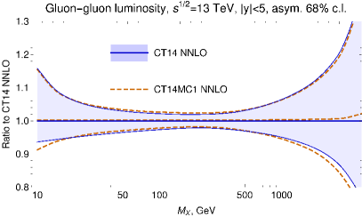
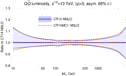
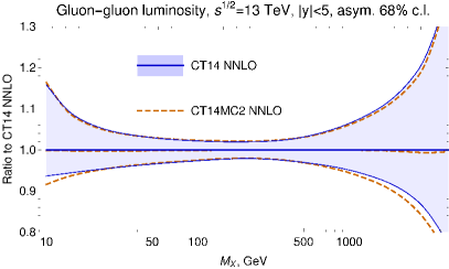
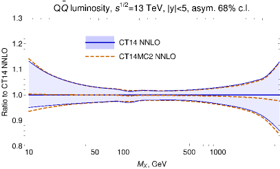
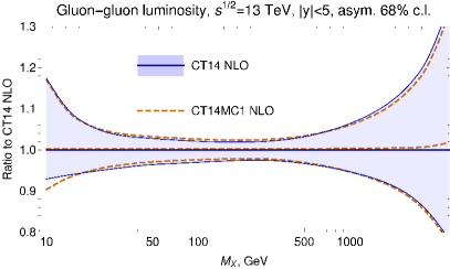
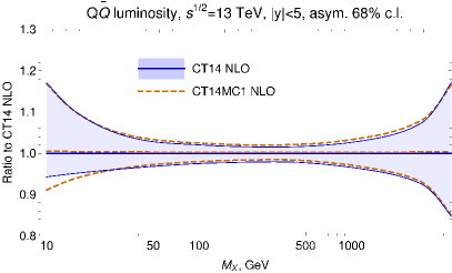
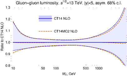
Taken together, Figs. 3, 4, and 5 demonstrate that our specifications for the construction of the replica PDFs do yield a satisfactory consistency with the central CT14 PDFs, and with the Hessian error PDFs. Therefore we expect that the uncertainties of cross sections calculated using the replica PDFs will agree with those based on error propagation via the Hessian PDFs. Comparisons of the most common LHC cross sections and cross section asymmetries, computed with the CT14 Hessian and MC PDFs, are presented at CT1 (a). By our design, in the regions where the PDFs are well constrained, the ensemble average of the predictions from either CT14MC1 or MC2 PDF set is expected to be close to the central prediction given by the central CT14 Hessian PDF set. Similarly, the asymmetric standard deviations given by the CT14MC PDF set are expected to be very close to the 68% c.l. uncertainties of the CT14 (Hessian) PDF error set, except when the value is very large (more than ) or small (less than ).
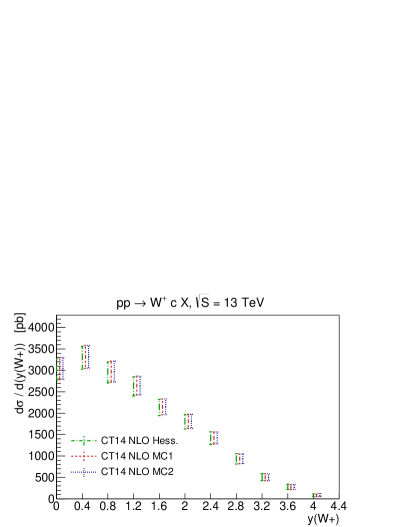
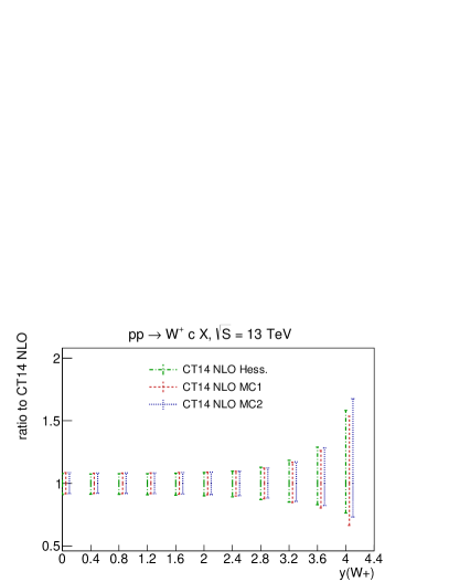
Some examples of cross sections are computed using the Applgrid fast interface Carli et al. (2010) for interpolation of NLO cross sections computed with the help of MadGraph_aMC@NLO Alwall et al. (2014), and aMCfast Bertone et al. (2014). The Applgrid input cross section tables are available at PDF from a study of cross sections based on PDF4LHC15 PDFs Gao et al. (2016); Butterworth et al. (2016). Specifically, we computed CT14 Hessian, MC1 and MC2 rapidity distributions with no or minimal experimental cuts for production , , , , production at the LHC 7,8, and 13 TeV. The renormalization and factorization scales are , , , , , respectively. is the scalar sum of transverse masses of final-state particles. For production, we neglect small contributions with initial-state or quarks. For NLO single-inclusive jet and dijet production, we use public APPLgrid files in the bins of ATLAS measurements Aad et al. (2012), created with the program NLOJET++ Nagy (2002, 2003). Similarly, the charge asymmetry in CMS experimental bins Chatrchyan et al. (2012, 2014) is computed with APPLgrid from Alekhin et al. (2015). An example of the cross sections on the website is shown in Fig. 9. For ease of comparisons, the PDF uncertainties are plotted both for the cross section values and for ratios to the central CT14 prediction.
III.2 Only an ensemble of MC replicas is meaningful
The results presented above provide a practical prescription for estimating asymmetric Hessian PDF uncertainties using an ensemble of Monte-Carlo replicas. As was already emphasized, some information about the primordial probability distribution in the global fit is lost in the process; however, the prescription is simple and provides a reasonable estimate in most cases. The method is most reliable and unique when the PDF uncertainty is small, meaning that the Taylor series converges fast. When the uncertainty is large, we see more variations, and several alternatives are conceivable. For example, our MC replicas are constructed so that their mean set coincides with the central set of the Hessian ensemble within numerical roundoff errors, as long as is not too large or too small. Instead, we could choose the central set of the Hessian ensemble to coincide with the median or mode sets of the MC replicas. Similarly, the PDF uncertainty bands may be defined by the positive and negative standard deviations discussed above, or by the boundaries of the 68% c.l. interval centered on the “central PDF set” chosen above. We have checked that the various prescriptions agree well at intermediate .
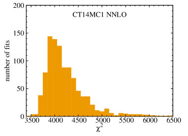
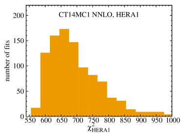
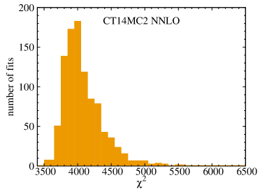
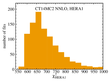
It is important to note that most replicas are poor fits to the hadronic data used in the global analysis; however, their averages and standard deviations defined in Sec. II provide excellent approximations for the Hessian central PDF set and 68% c.l. uncertainties. This is demonstrated in Fig. 10, showing histograms of values for the global data (3174 data points; left panel) and for the combined HERA-1 data (579 data points Aaron et al. (2010); right panel), for the 1000 replicas in the CT14 NNLO MC1 and MC2 ensembles. The vast majority of replicas yield very large values for the global data, and even for the single experiment. The random fluctuations of the individual replicas, which result in large values for any single replica, will largely cancel in the ensemble averages.
It is straightforward to understand why the result shown in Fig. 10 occurs. Imagine that we construct a -dimensional vector whose coordinates are given by random variates sampled from a standard normal distribution. The length of will often turn out to be significantly larger than 1. If those parameter values are used for the PDFs, will tend to be much larger than the minimal in the fit, especially if the number of dimensions is large. [Recall that the volume of an -dimensional unit ball vanishes in the limit of large . The vast majority of replicas will have several parameters far outside of the unit ball, i.e., away from the best fit by many standard deviations.]
The expected value of the length of can be easily found as
| (29) | |||||
The final approximation in (29) follows from Stirling’s formula for the gamma function. For , Eq. (29) gives ; that is, a typical displacement vector of a CT14 replica is more than five standard units in length. As a result, most replicas have a value that significantly exceeds the CT14 best-fit value of about 3250 for the global data and 590 for the HERA-1 data. If the standard deviation of the normal distribution is rather about 6 units (corresponding to at 90% c.l.), the average displacement vector corresponds to for the global data and (scaled down by 579/3174) for the HERA-1 data. This is far outside the typical for the distribution, given by , , or another common estimator! These estimates are in good agreement with the actual averages over the CT14 replicas, denoted as and equal in the case of the MC1 (MC2) NNLO ensembles to () for the global , and () for the HERA-1 .
It is interesting to note Thorne that the distribution for the CT14 MC replicas is quite similar in shape to the distributions for the global data of NNPDF replicas, obtained with an entirely different methodology Forte et al. (2002); Del Debbio et al. (2007); Ball et al. (2009, 2013, 2015). For example, for the four NNPDF3.0 NLO fits listed in Table 1 of Ref. Ball et al. (2016), the equivalent of our is 600-1000 units higher than the value for the average PDF set of all replicas.444The NNPDF table constructs from the values between theoretical predictions for an individual PDF replica and true (not fluctuated) experimental data. The average is over the ensemble of the NNPDF replicas. This can be qualitatively understood by noticing that the tensions between the individual experiments can be effectively accommodated by introducing a tolerance on the global at the 68% c.l. (Pumplin, 2010; Lai et al., 2010, sec. 7), and that the neural network parametrizations effectively have of order free parameters. This predicts , in fair agreement with the actual NNPDF3.0 outcomes. Individual replica PDFs thus cannot be considered as alternative PDFs with approximately the same accuracy as the central fit, or even with the accuracy of the Hessian error PDFs. The replica PDFs are meaningful only inside an ensemble, predictions based on them must be calculated by averaging over the ensemble.
IV Conclusions
The paper explored methods for the conversion of Hessian PDF error sets into Monte-Carlo replica PDFs. We observed that parameters of the PDFs approximately obey a multi-dimensional normal distribution in the vicinity of the global minimum. A statistical sample of MC replicas dependent on the probability distribution in the dimensional parameter space can be reconstructed under the Gaussian assumption from the distribution of the Hessian error PDFs on the ()-dimensional boundary of some confidence region enclosing the best fit. The CT14 Hessian error PDFs allow the user to estimate the PDF errors and account for the asymmetries due to mild deviations from the Gaussian shape and nonlinear nature of PDF parametrization. The CT14 PDFs are parameterized to be explicitly non-negative, as desired for obtaining sensible cross sections and uncertainties. In Sec. II we have generalized the algorithms for the generation of MC replicas and for the estimation of PDF uncertainties necessary to reproduce these features. Based on these results, we have generated two replica ensembles, designated as CT14MC1 and CT14MC2 PDFs. The average PDF sets and the asymmetric standard deviations of MC1 and MC2 closely reproduce the central sets and the 68% c.l. asymmetric uncertainties of the respective Hessian ensembles, cf. Sec. III. With the naive conversion, the mean set over the replicas may deviate from the central Hessian PDF set because of the truncation of Taylor series. After we apply a correction, the MC mean and central Hessian sets coincide, preventing potential discrepancies in the predictions. In addition, the CT14MC2 PDF replicas, obtained by sampling of a log-normal distribution, are explicitly non-negative.
To achieve good agreement between the CT14 Hessian and MC uncertainty bands, we recommend to construct the MC replicas by random sampling according to the algorithm summarized as Eqs. (19, 21, 24), and Sec. II.4. The central PDF set of such MC ensemble by construction coincides with the central Hessian PDF set. The PDF uncertainties for the MC ensemble are to be estimated by asymmetric standard deviations (25, 26), introduced as the counterparts for the master formulas (13, 14) for the Hessian asymmetric errors.
Our results in Sec. II clarify several aspects of the replica generation method that were not addressed in the previous work. Section III demonstrates that, in most of the range, where the PDF uncertainties are small, we observe good agreement between the CT14 Hessian, MC1, and MC2 error bands. In the extrapolation regions, where the linear approximations cease to be adequate, differences between the Hessian, MC1 and MC2 error bands are indicative of intrinsic ambiguities in the replica generation methods. At such extreme , they may affect the combination of the Hessian and MC ensembles, as in the recommended PDF4LHC procedure, or PDF replica re-weighting. These ambiguities require consideration when the converted replicas are utilized in PDF reweighting or PDF combinations. The positivity constraint on CT14 MC2 yields more physical behavior in poorly constrained intervals.
Once the MC replicas are generated by conversion, we examine their statistical properties in Sec. III.2. We point out that many individual MC replica sets yield poor , so only their statistical combinations, such as the mean, standard deviation, etc., are meaningful in applications. [The majority of MC replicas aren’t good fits, their combination is.] On the other hand, the distributions of MC replicas obtained by conversion (such as CT14 MC) or genetic algorithm (such as NNPDF) are very similar. This reflects the underlying commonalities of the two methods, leading to comparable PDF errors in the two approaches in spite of the distinct error definitions and fitting procedures.
The CT14 MC1 and MC2 ensembles at NNLO and NLO accuracy, together with a fast standalone driver program for their interpolation, can be downloaded at CT1 (b). They are also distributed as a component of the LHAPDF6 library LHA . A public C++ code mcgen is made available MCG for generation of MC PDF replicas using the normal, log-normal, and Watt-Thorne sampling methods, and with or without including the shifts. mcgen can be run as a standalone program or together with the Mathematica package MP4LHC for combination of PDF ensembles according to the meta-parametrization method Gao and Nadolsky (2014). After Hessian error PDF sets are read in the form of LHAPDF6 grids, output replicas are generated by random displacements of the Hessian replicas. Besides the replica generation, mcgen supports various algebraic operations with PDFs in the format of LHAPDF6 grid files, such as addition, averaging, and multiplication of the tables in which the PDF values are stored.
Acknowledgments
We thank R. Thorne for an instructive discussion about statistical properties of MC replicas. J.H., J.G., and P.N. thank the Kavli Institute for Theoretical Physics at Santa Barbara, CA and organizers of the “LHC Run II and Precision Frontier” research program for hospitality and productive atmosphere during completion of this paper. This research was supported in part by the National Science Foundation under Grants No. PHY-1410972 and PHY11-25915; by the U.S. Department of Energy under Contract No. DE-AC02-06CH11357 and Grants DE-SC0013681 and DE-SC0010129; and by the National Natural Science Foundation of China under Grant No. 11465018.
Definition of in CT fits
For completeness of the presentation, in this appendix, we reproduce the definition for the figure-of-merit function and the procedure for determination of PDF uncertainties in the CT14 fit, introduced in full detail in Refs. Lai et al. (2010); Gao et al. (2014); Dulat et al. (2016).
The most probable solutions for CT14 PDFs are found by minimization of a global log-likelihood function
| (30) |
which sums contributions from fitted experiments, and a contribution specifying theoretical conditions (“Lagrange Multiplier constraints”) imposed on some PDF parameters. In turn, the terms are given by
| (31) |
where
| (32) |
and
| (33) |
The contribution is a function of the PDF parameters and systematic nuisance parameters . For a -th data point, , and are the theoretical prediction, central experimental value, uncorrelated experimental uncertainty, and systematic correlation matrix, respectively.
The minimum of the function is found iteratively by the method of steepest descent using the program MINUIT. The boundaries of the 90% c.l. region around the minimum of , and the eigenvector PDF sets quantifying the associated uncertainty, are found by iterative diagonalization of the Hessian matrix Stump et al. (2001); Pumplin et al. (2001), which finds independent, or eigenvector, combinations of the PDF parameters . These combinations are denoted by , with the best-fit parameter combination corresponding to The 90% c.l. boundary around the best fit is determined by applying two tiers of criteria, based on the increase in the global summed over all experiments, and the agreement with individual experimental data sets Lai et al. (2010); Gao et al. (2014); Dulat et al. (2014b). The first type of condition demands that the global does not increase above the best-fit value by more than , where the 90% C. L. region corresponds to . The second condition introduces a penalty term in when establishing the confidence region, which quickly grows when the fit ceases to agree with any specific experiment within the 90% c.l. for that experiment. The effective function is scanned along each eigenvector direction until increases above the tolerance bound, or rapid growth due to the penalty is triggered.
The penalty term is constructed as
| (34) |
from the equivalent Gaussian variables that obey an approximate standard normal distribution independently of the number of data points in the experiment. Every is a monotonically increasing function of the respective given in Dulat et al. (2014b); Lewis (1988). The power is chosen so that sharply increases from zero when approaches 1.3, the value corresponding to 90% c.l. cutoff.
References
- Dulat et al. (2016) S. Dulat, T.-J. Hou, J. Gao, M. Guzzi, J. Huston, P. Nadolsky, J. Pumplin, C. Schmidt, D. Stump, and C.-P. Yuan, Phys. Rev. D93, 033006 (2016), eprint 1506.07443.
- Harland-Lang et al. (2015) L. A. Harland-Lang, A. D. Martin, P. Motylinski, and R. S. Thorne, Eur. Phys. J. C75, 204 (2015), eprint 1412.3989.
- Ball et al. (2015) R. D. Ball et al. (NNPDF), JHEP 04, 040 (2015), eprint 1410.8849.
- Abramowicz et al. (2015) H. Abramowicz et al. (ZEUS, H1), Eur. Phys. J. C75, 580 (2015), eprint 1506.06042.
- Alekhin et al. (2014) S. Alekhin, J. Blumlein, and S. Moch, Phys. Rev. D89, 054028 (2014), eprint 1310.3059.
- Accardi et al. (2016) A. Accardi, L. T. Brady, W. Melnitchouk, J. F. Owens, and N. Sato (2016), eprint 1602.03154.
- Pumplin et al. (2001) J. Pumplin, D. Stump, R. Brock, D. Casey, J. Huston, J. Kalk, H.-L. Lai, and W.-K. Tung, Phys. Rev. D65, 014013 (2001), eprint hep-ph/0101032.
- Giele and Keller (1998) W. T. Giele and S. Keller, Phys. Rev. D58, 094023 (1998), eprint hep-ph/9803393.
- Giele et al. (2001) W. T. Giele, S. A. Keller, and D. A. Kosower (2001), eprint hep-ph/0104052.
- Stump et al. (2001) D. Stump, J. Pumplin, R. Brock, D. Casey, J. Huston, J. Kalk, H.-L. Lai, and W.-K. Tung, Phys. Rev. D65, 014012 (2001), eprint hep-ph/0101051.
- Cooper-Sarkar (2002) A. M. Cooper-Sarkar, J. Phys. G28, 2669 (2002), eprint hep-ph/0205153.
- Pumplin et al. (2002) J. Pumplin, D. R. Stump, J. Huston, H. L. Lai, P. M. Nadolsky, and W.-K. Tung, JHEP 07, 012 (2002), eprint hep-ph/0201195.
- Nadolsky and Sullivan (2001) P. M. Nadolsky and Z. Sullivan, eConf C010630, P510 (2001), eprint hep-ph/0110378.
- Forte et al. (2002) S. Forte, L. Garrido, J. I. Latorre, and A. Piccione, JHEP 05, 062 (2002), eprint hep-ph/0204232.
- Del Debbio et al. (2007) L. Del Debbio, S. Forte, J. I. Latorre, A. Piccione, and J. Rojo (NNPDF), JHEP 03, 039 (2007), eprint hep-ph/0701127.
- Ball et al. (2009) R. D. Ball et al. (NNPDF), Nucl. Phys. B809, 1 (2009), eprint 0808.1231.
- Ball et al. (2013) R. D. Ball et al., Nucl. Phys. B867, 244 (2013), eprint 1207.1303.
- Watt and Thorne (2012) G. Watt and R. S. Thorne, JHEP 08, 052 (2012), eprint 1205.4024.
- Gao and Nadolsky (2014) J. Gao and P. Nadolsky, JHEP 07, 035 (2014), eprint 1401.0013.
- Carrazza et al. (2015a) S. Carrazza, S. Forte, Z. Kassabov, J. I. Latorre, and J. Rojo, Eur. Phys. J. C75, 369 (2015a), eprint 1505.06736.
- Carrazza et al. (2016) S. Carrazza, S. Forte, Z. Kassabov, and J. Rojo, Eur. Phys. J. C76, 205 (2016), eprint 1602.00005.
- Ball et al. (2011) R. D. Ball, V. Bertone, F. Cerutti, L. Del Debbio, S. Forte, A. Guffanti, J. I. Latorre, J. Rojo, and M. Ubiali (NNPDF), Nucl. Phys. B849, 112 (2011), [Erratum: Nucl. Phys.B855,927(2012)], eprint 1012.0836.
- Ball et al. (2012) R. D. Ball, V. Bertone, F. Cerutti, L. Del Debbio, S. Forte, A. Guffanti, N. P. Hartland, J. I. Latorre, J. Rojo, and M. Ubiali, Nucl. Phys. B855, 608 (2012), eprint 1108.1758.
- Carrazza et al. (2015b) S. Carrazza, J. I. Latorre, J. Rojo, and G. Watt, Eur. Phys. J. C75, 474 (2015b), eprint 1504.06469.
- Butterworth et al. (2016) J. Butterworth et al., J. Phys. G43, 023001 (2016), eprint 1510.03865.
- Lai et al. (2010) H.-L. Lai, M. Guzzi, J. Huston, Z. Li, P. M. Nadolsky, J. Pumplin, and C.-P. Yuan, Phys. Rev. D82, 074024 (2010), eprint 1007.2241.
- Gao et al. (2014) J. Gao, M. Guzzi, J. Huston, H.-L. Lai, Z. Li, P. Nadolsky, J. Pumplin, D. Stump, and C.-P. Yuan, Phys. Rev. D89, 033009 (2014), eprint 1302.6246.
- Belyaev et al. (2006) A. Belyaev, J. Pumplin, W.-K. Tung, and C.-P. Yuan, JHEP 01, 069 (2006), eprint hep-ph/0508222.
- Dulat et al. (2014a) S. Dulat, T.-J. Hou, J. Gao, J. Huston, P. Nadolsky, J. Pumplin, C. Schmidt, D. Stump, and C.-P. Yuan, Phys. Rev. D89, 113002 (2014a), eprint 1310.7601.
- Schmidt et al. (2014) C. Schmidt, S. Dulat, J. Gao, M. Guzzi, T.-J. Hou, J. W. Huston, P. Nadolsky, J. Pumplin, D. Stump, and C.-P. Yuan, PoS DIS2014, 146 (2014).
- Pumplin et al. (2009) J. Pumplin, J. Huston, H. L. Lai, P. M. Nadolsky, W.-K. Tung, and C.-P. Yuan, Phys. Rev. D80, 014019 (2009), eprint 0904.2424.
- Kenney and Keeping (1954) J. F. Kenney and E. S. Keeping, Mathematics of statistics (Van Nostrand, New York, 1954), chap. 4.7-4.9, pp. 50–54, 3rd ed., see also http://mathworld.wolfram.com/Mode.html.
- CT1 (a) http://http://hep.pa.msu.edu/cteq/public/ct14/MC/.
- (34) http://metapdf.hepforge.org/mcgen/.
- Campbell et al. (2007) J. M. Campbell, J. W. Huston, and W. J. Stirling, Rept. Prog. Phys. 70, 89 (2007), eprint hep-ph/0611148.
- Carli et al. (2010) T. Carli, D. Clements, A. Cooper-Sarkar, C. Gwenlan, G. P. Salam, F. Siegert, P. Starovoitov, and M. Sutton, Eur. Phys. J. C66, 503 (2010), eprint 0911.2985.
- Alwall et al. (2014) J. Alwall, R. Frederix, S. Frixione, V. Hirschi, F. Maltoni, O. Mattelaer, H. S. Shao, T. Stelzer, P. Torrielli, and M. Zaro, JHEP 07, 079 (2014), eprint 1405.0301.
- Bertone et al. (2014) V. Bertone, R. Frederix, S. Frixione, J. Rojo, and M. Sutton, JHEP 08, 166 (2014), eprint 1406.7693.
- (39) http://metapdf.hepforge.org/2016_pdf4lhc/.
- Gao et al. (2016) J. Gao, J. Huston, T.-J. Hou, P. M. Nadolsky, B. T. Wang, and K. P. Xie, in Proceedings of Les Houches 2015: Physics at TeV Colliders Standard Model Working Group Report, p. 13 (2016), eprint 1605.04692.
- Aad et al. (2012) G. Aad et al. (ATLAS), Phys. Rev. D86, 014022 (2012), eprint 1112.6297.
- Nagy (2002) Z. Nagy, Phys. Rev. Lett. 88, 122003 (2002), eprint hep-ph/0110315.
- Nagy (2003) Z. Nagy, Phys. Rev. D68, 094002 (2003), eprint hep-ph/0307268.
- Chatrchyan et al. (2012) S. Chatrchyan et al. (CMS), Phys. Rev. Lett. 109, 111806 (2012), eprint 1206.2598.
- Chatrchyan et al. (2014) S. Chatrchyan et al. (CMS), Phys. Rev. D90, 032004 (2014), eprint 1312.6283.
- Alekhin et al. (2015) S. Alekhin et al., Eur. Phys. J. C75, 304 (2015), eprint 1410.4412.
- Aaron et al. (2010) F. D. Aaron et al. (ZEUS, H1), JHEP 01, 109 (2010), eprint 0911.0884.
- (48) R. Thorne, in the summary talk of the Working Group 1, XXIV Workshop on Deep-Inelastic Scattering (DIS) and Related Subjects (DIS’2016), Hamburg, April 2016.
- Ball et al. (2016) R. D. Ball, V. Bertone, M. Bonvini, S. Carrazza, S. Forte, A. Guffanti, N. P. Hartland, J. Rojo, and L. Rottoli (NNPDF) (2016), eprint 1605.06515.
- Pumplin (2010) J. Pumplin, Phys. Rev. D81, 074010 (2010), eprint 0909.0268.
- CT1 (b) http://http://hep.pa.msu.edu/cteq/public/.
- (52) http://lhapdf.hepforge.org.
- Dulat et al. (2014b) S. Dulat, T.-J. Hou, J. Gao, J. Huston, J. Pumplin, C. Schmidt, D. Stump, and C.-P. Yuan, Phys. Rev. D89, 073004 (2014b), eprint 1309.0025.
- Lewis (1988) T. Lewis, Austral. J. Statist. 30A, 160 (1988).