Hashmod: A Hashing Method for Scalable 3D Object Detection

Abstract

We present a scalable method for detecting objects and estimating their 3D poses in RGB-D data. To this end, we rely on an efficient representation of object views and employ hashing techniques to match these views against the input frame in a scalable way. While a similar approach already exists for 2D detection, we show how to extend it to estimate the 3D pose of the detected objects. In particular, we explore different hashing strategies and identify the one which is more suitable to our problem. We show empirically that the complexity of our method is sublinear with the number of objects and we enable detection and pose estimation of many 3D objects with high accuracy while outperforming the state-of-the-art in terms of runtime.

1 Introduction

Scalable 3D object detection and pose estimation remains a hard problem to this day. The recent advent of low-cost RGB-D sensors boosted the research activity on object instance detection and 3D pose estimation even further, allowing state-of-the-art methods to robustly detect multiple objects and estimate their 3D poses even under high levels of occlusion. However, while image recognition and 2D object recognition methods can now scale to billions of images or millions of objects [26, 19, 10, 27], 3D object detection techniques are still typically limited to ten or so objects.

Some attempts to make 3D object detection scalable are based on local descriptions of 2D or 3D keypoints, since such descriptors can be matched in a sublinear manner via fast indexing schemes [24]. However, computing such descriptors is expensive [1, 38], and more importantly, they tend to perform poorly on objects without discriminative geometric or textural features. [5, 34, 4] also rely on recognition of densely sampled patches but are likely to work only when depth data is available. [20] uses a tree for object recognition, but still scales linearly in the number of objects, categories, and poses. Other approaches rely on part-based models [33, 29, 30], which are designed for category recognition rather than instance recognition, and little concern is given to the complexity, which is typically linear in the number of objects.

Our approach to 3D object detection is based on 2D view-specific templates which cover the appearance of the objects over multiple viewpoints [18, 25, 14, 17, 2]. Since viewpoints include the whole object appearance rather than just parts of it, they can generally handle objects with poor visual features, however they have not been shown to scale well with the number of images so far.  [35].

We are strongly influenced by [10] which showed impressive results in terms of 2D object detection by replacing convolutions of templates with constant-time hash table probes, parsing input images with 100,000 templates in about twenty seconds with respectable precision rates. We apply hash functions [12] to image descriptors computed over bounding boxes centered at each image location of the scene, so to match them efficiently against a large descriptor database of model views. In our work, we rely on the LineMOD descriptor [17], since it has been shown to work well for 3D object detection, although other descriptors such as HOG [8] could be certainly used as well.

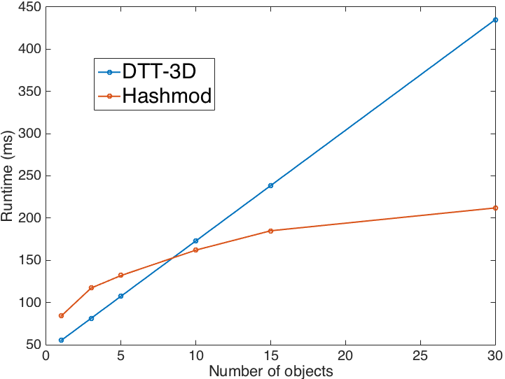
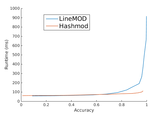
Our contribution is to present an efficient way of hashing such a descriptor: to this end, we explore different learning strategies to identify the one that is most suited to our problem. As shown in Figure 1, we outperform the state-of-the-art template matching method DTT-3D [31] by intelligently hashing our descriptors, achieving sublinear scalability.

Figure 1: Left: One frame of the ACCV12 dataset [17] augmented with our detections. Right: Average performance of our approach with a given amount of objects in the database. We clearly scale sublinearly and outperform the state-of-the-art [31] with more than 8 objects, enabling detection of many 3D objects at interactive runtimes.

2 Related work

3D object detection has a long history. Early works were based on edges [22, 16], then keypoint-based methods were shown to work reliably when distinctive features are available [26, 37, 36, 28] and robust schemes for correspondence filtering and verification are used [15, 1, 6]. Furthermore, they are also scalable since they can be reduced to searching nearest neighbors efficiently in their feature spaces [24, 19]. However, if such features are missing, which is actually the case for many daily objects, this approach becomes unreliable.

Template-based approaches then became popular. LineMOD [17] achieved robust 3D object detection and pose estimation by efficiently matching templated views with quantized object contours and normal orientations. In [31] the authors further optimize the matching via cascades and fine-tuned templates to achieve a notable run-time increase by a factor of 10. Nonetheless, these works still suffer from their linear time complexity. [23, 14, 32] show how to build discriminative models based on these representations using SVM or boosting applied to training data. While [23, 32] do not consider the pose estimation problem, [14] focuses on this problem only with a discriminatively trained mixture of HOG templates. Exemplars were also recently used for 3D object detection and pose estimation in [2], but the proposed approach still does not scale.

[5, 34] use forest-based voting schemes on local patches to detect and estimate 3D poses. While the former regresses object coordinates and conducts a subsequent energy-based pose estimation, the latter bases its voting on a scale-invariant LineMOD-inspired patch representation and returns location and pose simultaneously. [4] also uses Random Forests to infer object and pose, but via a sliding window through a depth volume. These methods remain slow, and it is not clear how they scale in performance with the number of objects.

Over the last years, hashing-based techniques became quite popular for large-scale image classification since they allow for immediate indexing into huge datasets. Apart from many works that focused on improving hashing of real-valued features into more compact binary codes [21, 13], there has been ongoing research on applying hashing in a sliding window scenario for 2D object detection: [10] applies hashing on HOG descriptors computed from Deformable Part Models to scale to 100,000 2D object classes. [3] presents a scalable object category detector by representing HOG sparsely with a set of patches which can be retrieved immediately.

Hashing has also been used for 3D object detection: [9] hashes paths over edgelets in color images and allows for real-time 3D object detection, however the output remains in terms of 2D locations only. [7] applies uniform quantization to edge-based descriptors to immediately look up approximate nearest neighbors. Here we instead prefer hashing techniques in conjunction with a learning scheme since it tends to provide better accuracy by taking the actual data variety into account.

3 Hashing for Object Recognition and 3D Pose Estimation

Figure 2: Left: As in  [17], we compute LineMOD descriptors for synthetically rendered views sampled on hemispheres of several radii. Right: One such synthetic view of the ‘lamp’ object overlaid with the fixed grid for matching and the color-coded quantized orientations of image gradients and 3D normals used to compute the descriptor.

Figure 3: Visualization of the hashing pipeline with one hash function $h$ and a key length of $b=6$. At each sliding window’s position we extract a LineMOD descriptor $\mathbf{x}$ and sample certain orientations at specific positions to form a short binary string $h(\mathbf{x})$. This serves as an index into the pre-filled hash table to retrieve candidate views for further matching. Both the sample positions and orientations for $h$ are learned.

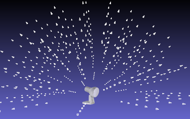
Given a database of $M$ objects, we synthetically create $N$ views for each object from poses regularly sampled on a hemisphere of a given radius, as shown in Figure 2. From this, we compute a set $\mathcal{D}$ of $d$-dimensional binary descriptors:

$$\mathcal{D}=\left\{\mathbf{x}_{1,1},...,\mathbf{x}_{M,N}\right\}\;\;,$$ (1)

where $\mathbf{x}_{i,j}\in\mathbb{B}^{d}$ is the descriptor for the $i$-th object seen under the $j$-th pose. As already mentioned, we use LineMOD in practice to compute these descriptors. The LineMOD descriptor is a vector of integers between 0 and 16 and for each pixel it is either set to 0 when there is no significant image gradient or depth data present or otherwise set to a value to represent a quantized orientation of either an image gradient (1-8) or 3D normal (9-16). We concatenate the binary representation of these integer values to obtain the binary strings $\mathbf{x}_{i,j}$. In the remainder of this work we will use the terms views, templates, and descriptors as synonyms.

Figure 3 gives an overview of our pipeline. As usually done in template-based approaches, we parse the image with a sliding window looking for the objects of interest. We extract at each image location the corresponding descriptor $\mathbf{x}$. If the distance between $\mathbf{x}$ and its nearest neighbor $\mathbf{x}_{i,j}$ in $\mathcal{D}$ is small enough, it is very likely that the image location contains object $i$ under pose $j$. As discussed in the introduction, we want to perform this (approximate) nearest neighbor search by hashing the descriptors. Therefore, we explore different strategies for building the hashing functions. This is done in the offline stage described below.

Also note that we tackle the issue of object scale and views of different 2D sizes by dividing the views up into clusters $\mathcal{D}_{s}\subset\mathcal{D}$ of similar scale $s$. This leads to $s$ differently-sized sliding windows during testing which extract differently-sized descriptors on which to perform the hashing. Moreover, to increase detection rates, we assign a pre-defined number of hash functions per window such that they relate to random but overlapping subsets of $\mathcal{D}_{s}$. During testing, we evaluate all sliding windows with their associated hashing functions, union their retrieved views and conduct subsequent matching. Lastly, we determined a good compromise for the key lengths by setting for each scale $s$ the key length $b_{s}:=\lfloor\log_{2}(|\mathcal{D}_{s}|)\rfloor$.

3.1 Selecting the Hashing Keys

During our offline stage, we learn several hashing functions $h$ [12]. As shown in Figure 3, the purpose of each function is to immediately index into a subset, often called a “bucket”, of $\mathcal{D}$ when applied to a descriptor $\mathbf{x}\in\mathbb{B}^{d}$ during testing. These buckets are filled with descriptors from $\mathcal{D}$ with the same hash value so that we can restrict our search for the nearest neighbor of $\mathbf{x}$ to the bucket retrieved via the hashing function instead of going through the complete set $\mathcal{D}$. It is very likely, but not guaranteed, that the nearest neighbor is in at least one of the buckets returned by the hashing functions.

In practice, a careful selection of the hashing functions is important for good performance. Since the descriptors $\mathbf{x}$ are already binary strings, we design our hashing functions $h(\mathbf{x})$ to return a short binary string made of $b$ bits directly extracted from $\mathbf{x}$. This is a very efficient way of hashing and we will refer to these short strings as hash keys.

There is a typical trade-off between accuracy and speed: we want to retrieve only a handful of descriptors at each image location and the number of retrieved elements is governed by the hash key length and the distribution of the descriptors among the buckets. Since we use $b$ bits for the hash table, we span a table with $2^{b}$ buckets. If a key is too short, the number of buckets is too small and we store overproportionally many descriptors per bucket, increasing subsequent matching time after retrieval. If the key is too large, we might be more prone to noise in the bitstrings which may lead to wrong buckets, rendering false negatives more probable during testing. We thus want to select these $b$ bits in a way such that we maximize the odds of finding the nearest neighbors of the input descriptors in the buckets while keeping the total amount of retrieved views to a minimum.

An exhaustive evaluation of all the possible bit selections to build the hash keys is clearly intractable. We experimented with the following variants:

Randomness-based selection (RBS)

Given a set of descriptors, we select the $b$ bits randomly among all possible $d$ bits. As we will see later on, this selection strategy yields bad results since some bits are more discriminant than others in our template representation. Nonetheless, it provides us with a weak baseline we can compare to and it outlines the importance of a more sophisticated approach towards hash learning.

Probability-based selection (PBS)

For this strategy, we focus on the bits for which the probabilities of being $0$ and $1$ are close to $0.5$ with a given set of descriptors. We therefore rank each bit $B$ according to its entropy $E=p(B={\tt 0})\ln p(B={\tt 0})+p(B={\tt 1})\ln p(B={\tt 1})$ and take the best $b$. This strategy provides a high accuracy since it focuses on the most discriminant bits. However, later evaluation will reveal that this strategy results in a high variance in the number of elements per bucket, rendering PBS inefficient in terms of runtime.

Tree-based selection (TBS)

This strategy is inspired by greedy tree growing for Randomized Forests. Starting with a set of descriptors at the root, we determine the bit that splits this set into two subsets with sizes as equal as possible, and use it as the first bit of the key. For the second bit, we decide for the one that splits those two subsets further into four equally-sized subsets and so forth. We stop if $b$ bits have been selected or one subset becomes empty. This procedure alone yields a balanced tree with leafs of similar numbers of elements. Each hash key can be regarded as a path down the tree and each leaf represents a bucket. Note that such a balanced repartition ensures retrieval and matching at a constant speed. Formally, the $j$-th bit $B$ of the key is selected by solving:

$$\operatorname*{arg\,min}_{B}\sum_{i}\Big{|}|\mathcal{S}_{L}^{B}(N_{i})|-|\mathcal{S}_{R}^{B}(N_{i})|\Big{|}\;\;,$$ (2)

where $N_{i}\subset\mathcal{D}$ is the set of descriptors contained by the $i$-th node at level $j$, and $\mathcal{S}_{\{L,R\}}^{B}(N_{i})$ are the two subsets of $N_{i}$ that go into the left and right child induced by splitting with $B$.

Tree-based selection with view scattering (TBV)

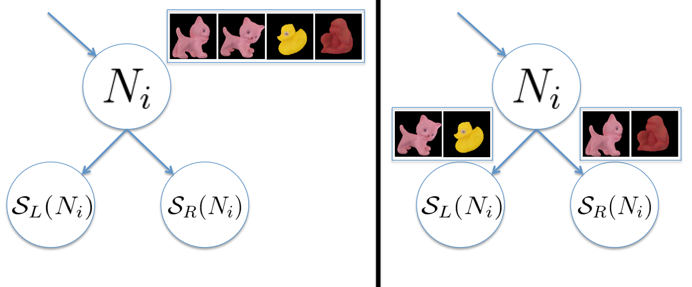
We now further adapt the TBS strategy to our problem: as illustrated in Figure 4, to improve detection rates we favor similar views of the same object to go into different branches. The idea behind this strategy is to reduce misdetections due to noise or clutter in the descriptor. If an extracted hash has a polluted bit and thus points to a wrong bucket, we might not retrieve the best view but still could recover from a similar view that we stored in the bucket the polluted hash points to. This strategy improves the robustness of the TBS retrieval, resulting in a consistently higher recall. We optimize the previous criterion with an additional term:

$$\operatorname*{arg\,min}_{B}\frac{1}{|N_{i}|}\sum_{i}\Big{|}|\mathcal{S}_{L}^{B}(N_{i})|-|\mathcal{S}_{R}^{B}(N_{i})|\Big{|}+\frac{1}{|N_{i}|^{2}}\Big{(}P(\mathcal{S}_{L}^{B}(N_{i}))+P(\mathcal{S}_{R}^{B}(N_{i}))\Big{)}\;\;,$$ (3)

where the second term penalizes close views falling into the same side of the split. We define the penalty function $P(\cdot)$ as:

$$P(N):=\sum_{\mathbf{x}\in N}\sum_{\mathbf{y}\in N}\mathbb{I}(\mathbf{x},\mathbf{y})\cdot\begin{cases}1,\text{ if }\cos^{-1}(|\langle q_{\mathbf{x}},q_{\mathbf{y}}\rangle|)<\tau\\ 0,\text{ otherwise}\;\;,\end{cases}$$ (4)

where $\mathbb{I}(\mathbf{x},\mathbf{y})$ indicates if descriptors $\mathbf{x}$ and $\mathbf{y}$ encode views of the same object and $q_{\mathbf{x}},q_{\mathbf{y}}$ are the quaternions associated with the rotational part of the descriptors’ poses. We set the proximity threshold $\tau=0.3$ empirically according to our viewpoint sampling.

Figure 4: The TBV strategy encourages descriptors for similar views to fall into different buckets. This increases the chances to find a close descriptor when parsing the buckets.

3.2 Remarks on the Implementation

For selecting the hash keys, we rely on the descriptors after ‘bit spreading’ of LineMOD [17], which makes the descriptors robust to small translations and deformations in a neighborhood of $T$ pixels. It increases the spatial overlap of quantized features and allows for a better descriptor separability. For matching itself we used the unspreaded templates.

Furthermore, after one bit has been selected, we disallowed all bits closer than $T$ to be selected for the same LineMOD value. This forces the bit selection to take different values and positions into account, as we sometimes observed an accumulation of selected bits encoding the same orientation in one area which could lead to bad recognition rates.

For efficiency, we conduct the matching analogously to [31] on a fixed grid. As opposed to [17], we do not use a robust cosine-based similarity score but count the bits after ANDing the descriptors and dividing by the number of grid points falling on the view foreground.

4 Evaluation

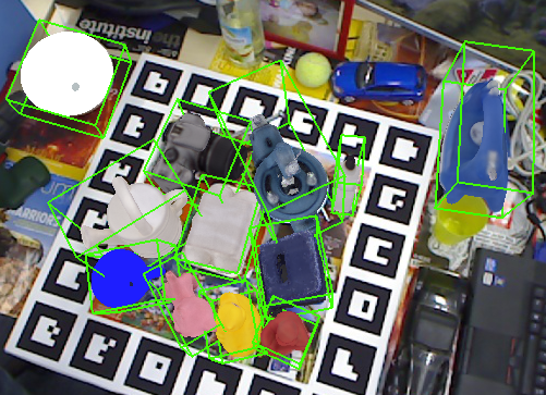
We ran our method on the LineMOD ACCV12 dataset [17] consisting of 15 objects and followed the exact same protocol to create an equidistant viewpoint sampling. Furthermore, scale and in-plane rotations were sampled accordingly to cover a pre-defined 6D pose space, resulting in exactly $N=3115$ views per object.

We followed [17] and spread the quantized values in a small neighborhood of $T=8$ pixels which makes the representation robust and allows to check only every $T$-th image position. Furthermore, we use the same post-processing: after retrieval/matching, we sort the candidates according to their score and run a rough color check to discard obvious outliers. We conduct a fast voxel-based ICP [11] and reject candidates if the average euclidean error is too large. Finally, the first $n=10$ survivors are projected onto the scene to run a finer ICP together with a depth check to decide for the best match. We use the same evaluation criteria with a distance factor of $k_{m}=0.1$ to decide for a hit or miss.

The computational cost during testing is modest: the whole system runs on a single CPU-core—apart from the post-processing where the depth check projections use OpenGL calls—, uses no pyramid scheme and the hash tables take up less than 1 MB.

Figure 5: Examples of accuracies and runtimes for different strategies and a varying database size. Left column: for the ‘ape’ sequence. Right column: for the ‘lamp’ sequence. The number in the legend for each strategy denotes the amount of hash keys per window.

Seq / Objs	1	3	5	10	15
ape	96.1% / 73ms	95.1% / 127ms	96.8% / 134ms	94.1% / 164ms	95.6% / 180ms
bvise	92.8% / 83ms	95.4% / 117ms	91.2% / 128ms	92.3% / 181ms	91.2% / 192ms
bowl	99.3% / 84ms	98.8% / 114ms	98.6% / 123ms	98.1% / 156ms	98.6% / 184ms
cam	97.8% / 75ms	96.9% / 111ms	95.3% / 129ms	94.8% / 162ms	95.2% / 174ms
can	92.8% / 81ms	91.6% / 112ms	93.7% / 119ms	93.9% / 158ms	91.8% / 171ms
cat	98.9% / 99ms	97.2% / 117ms	97.4% / 138ms	95.8% / 164ms	96.1% / 188ms
cup	96.2% / 65ms	96.0% / 100ms	95.3% / 117ms	94.5% / 144ms	98.6% / 194ms
driller	98.2% / 106ms	97.8% / 135ms	98.1% / 162ms	97.6% / 171ms	95.1% / 190ms
duck	94.1% / 74ms	90.8% / 122ms	90.7% / 124ms	91.5% / 161ms	92.9% / 179ms
eggbox	99.9% / 68ms	99.9% / 103ms	99.9% / 115ms	99.9% / 151ms	99.9% / 174ms
glue	96.8% / 100ms	96.2% / 131ms	94.4% / 154ms	95.3% / 166ms	95.4% / 175ms
hpuncher	95.7% / 97ms	95.3% / 118ms	95.8% / 142ms	95.2% / 162ms	95.9% / 183ms
iron	96.5% / 101ms	94.8% / 122ms	95.0% / 141ms	95.5% / 167ms	94.3% / 203ms
lamp	98.4% / 93ms	95.4% / 114ms	95.3% / 137ms	96.1% / 172ms	94.9% / 179ms
phone	93.3% / 90ms	94.6% / 126ms	94.5% / 133ms	91.7% / 167ms	91.3% / 198ms
TBV Average	96.5% / 83ms	95.7% / 117ms	95.5% / 131ms	94.9% / 162ms	95.1% / 184ms
DTT-3D [31]	97.2% / 55ms	97.2% / 81ms	97.2% / 107ms	97.2% / 173ms	97.2% / 239ms
LineMOD [17]	96.6% / 119ms	96.6% / 273ms	96.6% / 427ms	96.6% / 812ms	96.6% / 1197ms

Table 1: Accuracy and runtime per frame for our whole pipeline with the TBV strategy, DTT-3D and LineMOD for the whole dataset with a varying number of trained and loaded objects. With only a few objects, DTT-3D is faster than our approach. However, its complexity increases linearly with the database size, allowing us to overtake when the number of objects becomes higher. Note that the dataset only provides groundtruth for one object per frame.

Different learning strategies.

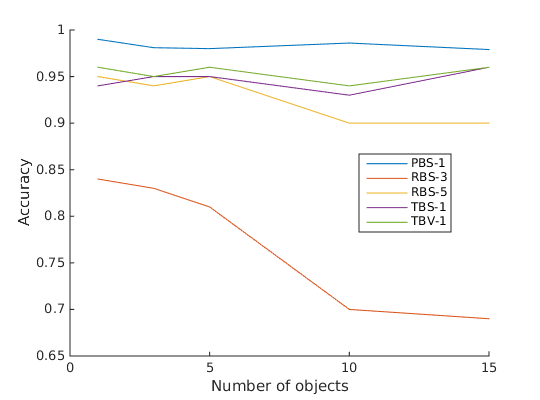
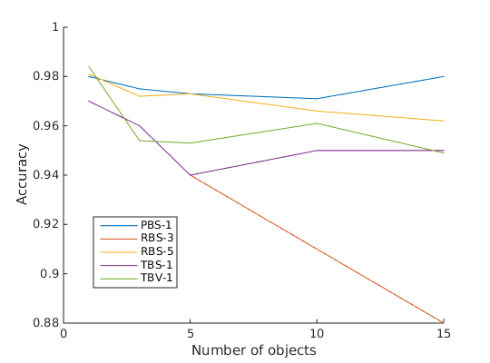
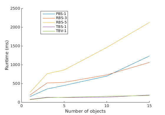
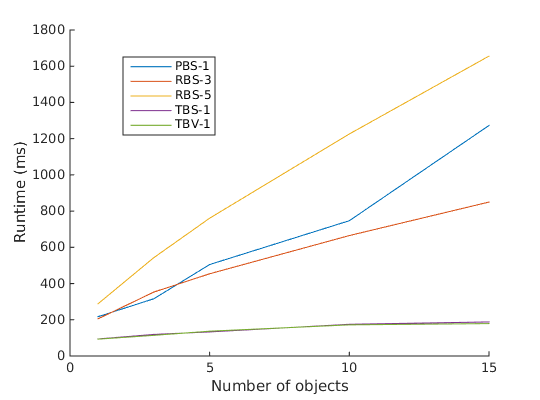
We learned the hashing for each sequence/objects configuration by grouping the object of interest together with a random subset of the remaining ones. An exception is the case for 15 objects where we built the hash tables once and used them for all tests. A summary of our evaluation is given in Figure 5. Note that we conducted our experiments with a varying amount of hash tables per window/scale for each strategy but only plot the most insightful to not clutter the graphs and save space. The behavior was similar across the whole dataset and we thus present results for all strategies only on two sequences and then restrict ourselves to the best strategy thereafter for a more detailed analysis.

The RBS strategy was clearly the weakest one. This is because RBS managed a poor separation of descriptors: since the key bits were chosen randomly, most descriptors were assigned a hash value of pure zeros and were put into the first bucket while the rest of the hash table was nearly empty. This resulted during testing in either hitting an arbitrary bucket with no elements or the 0-bucket with a high amount of retrieved views, approximating an exhaustive search at that image location which increased matching time. It only started to detect accurately with multiple tables per window at the expense of very high runtimes.

Not surprisingly, PBS nearly always managed to correctly detect the object—limited only by our matching threshold—while achieving similar runtimes as RBS with 3 tables per window. An inspection of the hashes revealed that PBS led to multiple large buckets where descriptors concentrated and if one of those buckets was hit, it was very likely that it contained the correct view. Nonetheless, PBS does not take advantage of all available buckets as some of them remain empty and therefore still exhibits a linear runtime growth. Using more tables for RBS was just slightly increasing runtime and accuracy.

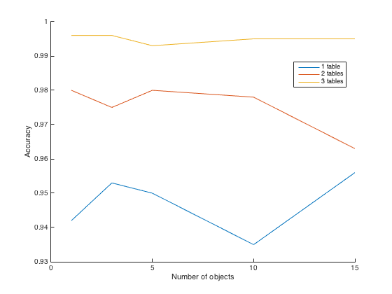
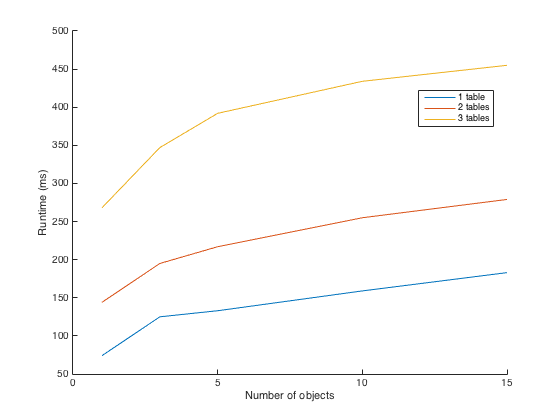
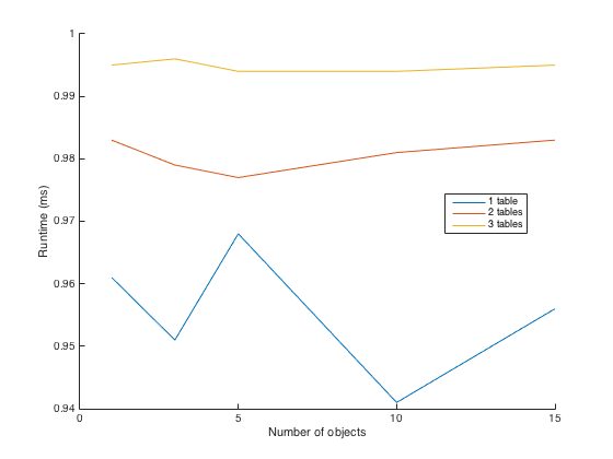
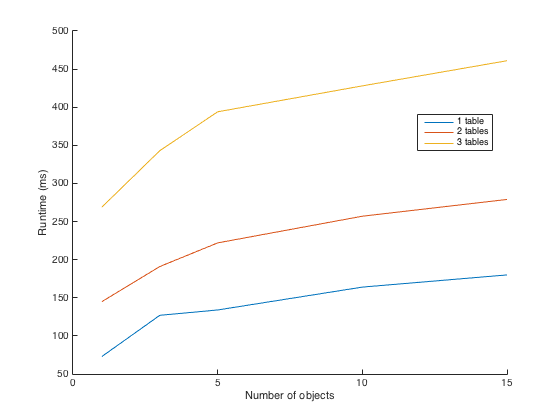
For both TBV and TBS the most interesting observation is their sublinear growth in runtime. Enforcing the tables to be filled equally results in an obvious drop in the amount of retrieved views. Nonetheless, both strategies yield already good accuracies with one table per window and TBV was able to outperform TBS usually with around $2\%$ in accuracy since otherwise missed views could be retrieved and ICP-refined to the same correct pose from a similar view in another bucket.

Comparison to related methods.

Since TBV supplies us with a sublinear runtime growth and acceptably high accuracies, we settle for this strategy and show more detailed results in Table 1. We are able to consistently detect at around $95\%-96\%$ accuracy on average which is slightly worse than LineMOD and DTT-3D. However, we are always faster than LineMOD and overtake DTT-3D at around 8 objects where our constant-time hashing overhead becomes negligible and the methods’ time complexities dominate. This is important to stress since real scalability comes from a sublinear growth. Additionally, we show more clearly the scalability of our approach when increasing the amount of descriptors: since the dataset consists of only 15 objects, yielding 46,725 descriptors, we created further 46,725 descriptors by drawing each bit from its estimated distribution, thus enlarging our database artificially to 30 objects. Figure 1 shows a graph of our runtimes in comparison to DTT-3D. For the latter, we extrapolated the values given the authors’ timings. The gap in runtime shows our superiority when dealing with many objects and views.

Sublinear retrieval and matching.

Figure 6: Left: Accuracy versus runtime on the ‘driller’-sequence with TBV hash keys and LineMOD with a set of decreasing matching thresholds. Both methods achieve higher accuracies with a lower threshold although we only retrieve a fraction of views, making our runtime increase marginal. Right: Matching ratios for an increasing number of objects using TBV hash keys. The obvious decreasing trend allows us to scale with the number of objects.

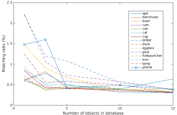
After retrieval, we conduct template matching together with an object-dependent threshold. Although this parameter is of importance to balance runtime versus accuracy, we are less prone to ill settings in comparison to LineMOD since at each position we only retrieve a tiny subset of candidates, as shown in Figure 6 (left). Obviously, the small set of retrieved views most often contains the correct one, leading to good accuracies while keeping the runtime low. Furthermore, the ratio of total conducted matchings on an image of size $W\times H$,

$$\#\text{retrieved templates}\hskip 2.84544pt/\hskip 2.84544pt\frac{\#\text{templates in database}\cdot W\cdot H}{T\cdot T}$$ (5)

stays small as shown in Figure  6 (right) and explains our improvement in comparison to an exhaustive search: while increasing the object database size, the ratio grows smaller. It is this trend of decay that allows us to scale sub-linearly with the number of objects/views.

5 Conclusion and Acknowledgment

We presented a novel method for 3D object detection and pose estimation which employs hashing for efficient and truly scalable view-based matching against RGB-D frames. We showed that we outperform the state-of-the-art in terms of speed while being able to achieve comparable accuracies on a challenging dataset. It would be interesting to invest further effort into alternative hash learning schemes, different feature representations and extend the experiments to other challenging multi-object datasets. The authors would also like to thank Toyota Motor Corporation for supporting and funding the work.

Supplementary material

6 Different learning strategies

As mentioned in the paper, the performance of the hash tables is governed by the length of the key, i.e. the number of buckets that are spanned, and by the distribution of the descriptors in the buckets. In Figure 7 we had a key length of $b=7$ which provided us with a table of 128 possible buckets. To relate to the discussed results in the evaluation, we present here the resulting tables acquired by each strategy. Furthermore, we provide 3 important quantities for each table: the actual number of used buckets, the largest number of descriptors that is in one bucket as well as the standard deviation computed over all non-empty buckets.

Note that we did not necessarily take the tables from the same scale, since both TBV and TBS terminate prematurely if one leaf becomes empty after splitting, reducing the key length. We rather took the tables from different scales such that we can present each table spanning the same number of buckets to give a nicer qualitative comparison. Nonetheless, the behavior is the same across all objects and scales for each strategy, making our comparison unproblematic.

Apparently, RBS produced by far the largest disparity in bucket sizes where the largest, storing 76 descriptors, is also at the same time the mentioned 0-bucket. The remaining used 12 buckets are rather small and the other 115 are completely empty, leading to a high standard deviation. Hitting the 0-bucket retrieves a lot of descriptors, shooting up runtime unnecessarily while otherwise the method retrieves virtually nothing at all when hitting any other bucket.

PBS already uses more buckets than RBS and creates a more balanced separation into multiple larger sets. The best results are however obtained with our tree-based selection strategies that provide us with a good distribution among the buckets, i.e. small bucket sizes together with a small standard deviation. In the optimal case, the standard deviation would be zero and the buckets’ usage would equal an uniform distribution.

       

Figure 7: For each strategy, we depict a filled hash table that we computed for the ‘benchvise’. From top to bottom: RBS, PBS, TBS, TBV. Note that the height for each hash table is normalized, skewing the comparison optically.

7 Matching thresholds

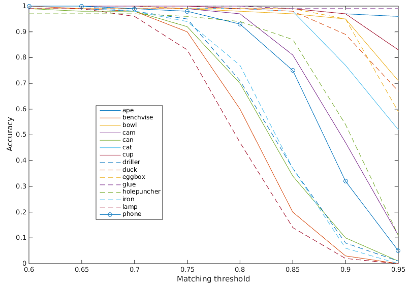
In order to determine each object-dependent matching threshold for our grid-based similarity score, we conducted a sweep over the thresholds for each sequence and fixed them such that each object would be found at least with an average accuracy of 98% in an exhaustive search scenario. See Figure 8 for the graphs.

Figure 8: Average accuracy for each object on its associated sequence with different matching thresholds when running an exhaustive search.

8 Different number of tables per scale

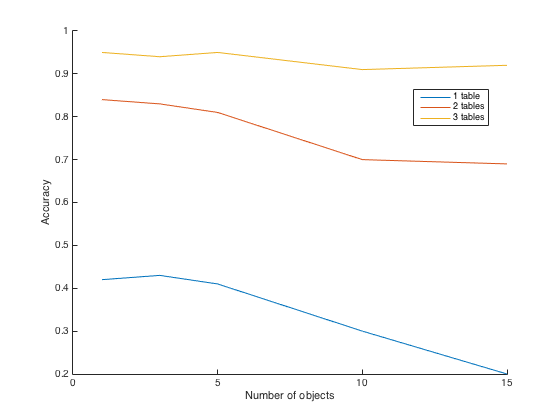
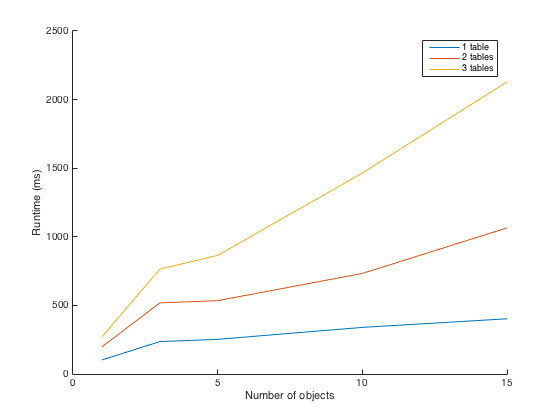
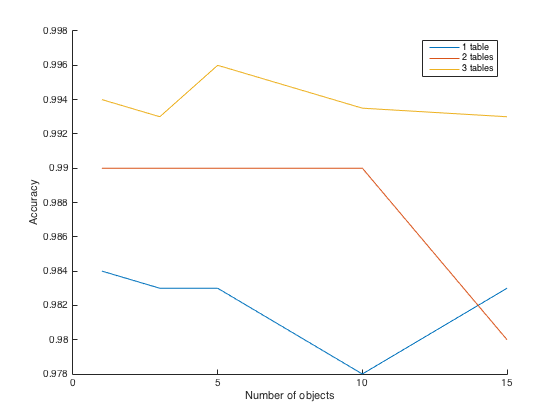
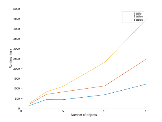
We evaluated each strategy with a different amount of trained hash tables per scale in Figure 9. For this, the descriptors for each scale were subdivided into multiple overlapping groups and then one table was responsible for indexing into one of them. As we can observe on the next page, increasing the amount of tables always leads to better recognition at the expense of higher runtimes. Except for the RBS strategy which would have needed even more tables still, all methods experienced a saturation in detection accuracy for the ‘ape’ around $99.5\%$. In light of to these results, we settled for TBV and one table per scale because it allowed us to be faster than DTT-3D with a comparable accuracy.

Figure 9: Plotting the behavior for each strategy on the ‘ape’ sequence when the amount of tables per scale increases. From top to bottom: RBS, PBS, TBS, TBV.

References

- [1] A. Aldoma, F. Tombari, J. Prankl, A. Richtsfeld, L. Di Stefano, and M. Vincze. Multimodal Cue Integration through Hypotheses Verification for RGB-D Object Recognition and 6DOF Pose Estimation. In ICRA, 2013.
- [2] M. Aubry, D. Maturana, A. Efros, B. Russell, and J. Sivic. Seeing 3D Chairs : Exemplar Part-Based 2D-3D Alignment Using a Large Dataset of CAD Models. In CVPR, 2014.
- [3] Y. Aytar and A. Zisserman. Immediate, Scalable Object Category Detection. In CVPR, 2014.
- [4] U. Bonde, V. Badrinarayanan, and R. Cipolla. Robust Instance Recognition in Presence of Occlusion and Clutter. In ECCV, 2014.
- [5] E. Brachmann, A. Krull, F. Michel, S. Gumhold, J. Shotton, and C. Rother. Learning 6D Object Pose Estimation Using 3D Object Coordinates. In ECCV, 2014.
- [6] A. G. Buch, Y. Yang, N. Krüger, and H. G. Petersen. In Search of Inliers : 3D Correspondence by Local and Global Voting. In CVPR, 2014.
- [7] H. Cai, T. Werner, and J. Matas. Fast Detection of Multiple Textureless 3D Objects. In ICVS, 2013.
- [8] N. Dalal and B. Triggs. Histograms of Oriented Gradients for Human Detection. In CVPR, 2005.
- [9] D. Damen and P. Bunnun. Real-Time Learning and Detection of 3D Texture-Less Objects: A Scalable Approach. In BMVC, 2012.
- [10] T. Dean, M. Ruzon, M. Segal, J. Shlens, S. Vijayanarasimhan, and J. Yagnik. Fast, Accurate Detection of 100,000 Object Classes on a Single Machine. In CVPR, 2013.
- [11] A. Fitzgibbon. Robust Registration of 2D and 3D Point Sets. In BMVC, 2001.
- [12] A. Gionis, P. Indyk, and R. Motwani. Similarity Search in High Dimensions via Hashing. In VLDB, 1999.
- [13] Y. Gong, S. Lazebnik, A. Gordo, and F. Perronnin. Iterative Quantization: A Procrustean Approach to Learning Binary Codes for Large-Scale Image Retrieval. PAMI, 2013.
- [14] C. Gu and X. Ren. Discriminative Mixture-Of-Templates for Viewpoint Classification. In ECCV, 2010.
- [15] Q. Hao, R. Cai, Z. Li, L. Zhang, Y. Pang, F. Wu, and Y. Rui. Efficient 2D-To-3D Correspondence Filtering for Scalable 3D Object Recognition. CVPR, 2013.
- [16] C. Harris. Tracking with Rigid Objects. MIT Press, 1992.
- [17] S. Hinterstoisser, V. Lepetit, S. Ilic, S. Holzer, G. Bradsky, K. Konolige, and N. Navab. Model Based Training, Detection and Pose Estimation of Texture-Less 3D Objects in Heavily Cluttered Scenes. In ACCV, 2012.
- [18] D. Hoiem and S. Savarese. Representations and Techniques for 3D Object Recognition and Scene Interpretation. Morgan & Claypool Publishers, 2011.
- [19] H. Jégou, M. Douze, and C. Schmid. Product Quantization for Nearest Neighbor Search. PAMI, 33(1), 2011.
- [20] K. Lai, L. Bo, X. Ren, and D. Fox. A Scalable Tree-Based Approach for Joint Object and Pose Cecognition. In AAAI, 2011.
- [21] G. Lin, C. Shen, Q. Shi, A. V. D. Hengel, and D. Suter. Fast Supervised Hashing with Decision Trees for High-Dimensional Data. In CVPR, 2014.
- [22] D. G. Lowe. Fitting Parameterized Three-Dimensional Models to Images. PAMI, 13(5):441–450, June 1991.
- [23] T. Malisiewicz, A. Gupta, and A. Efros. Ensemble of Exemplar-SVMs for Object Detection and Beyond. In ICCV, 2011.
- [24] M. Muja and D. Lowe. Scalable Nearest Neighbour Methods for High Dimensional Data. PAMI, 2014.
- [25] S. Nayar, S. Nene, and H. Murase. Real-Time 100 Object Recognition System. In ICRA, 1996.
- [26] D. Nistér and H. Stewénius. Scalable Recognition with a Vocabulary Tree. In CVPR, 2006.
- [27] M. Norouzi, A. Punjani, and D. J. Fleet. Fast Exact Search in Hamming Space with Multi-Index Hashing. PAMI, 36(6):1107–1119, 2014.
- [28] K. Pauwels, L. Rubio, J. Diaz, and E. Ros. Real-Time Model-Based Rigid Object Pose Estimation and Tracking Combining Dense and Sparse Visual Cues. In CVPR, 2013.
- [29] N. Payet and S. Todorovic. From Contours to 3D Object Detection and Pose Estimation. In ICCV, 2011.
- [30] B. Pepik, P. Gehler, M. Stark, and B. Schiele. 3D2PM-3D Deformable Part Models. In ECCV, 2012.
- [31] R. Rios-Cabrera and T. Tuytelaars. Discriminatively Trained Templates for 3D Object Detection: A Real Time Scalable Approach. In ICCV, 2013.
- [32] R. Rios-Cabrera and T. Tuytelaars. Boosting Masked Dominant Orientation Templates for Efficient Object Detection. CVIU, 120:103–116, 2014.
- [33] S. Savarese and L. Fei-Fei. 3D Generic Object Categorization, Localization and Pose Estimation. In ICCV, 2007.
- [34] A. Tejani, D. Tang, R. Kouskouridas, and T.-K. Kim. Latent-Class Hough Forests for 3D Object Detection and Pose Estimation. In ECCV, 2014.
- [35] F. Tombari, A. Franchi, and L. D. Stefano. BOLD Features to Detect Texture-Less Objects. In ICCV, 2013.
- [36] F. Tombari, S. Salti, and L. Di Stefano. Unique Signatures of Histograms for Local Surface Description. In ECCV, 2010.
- [37] D. Wagner, G. Reitmayr, A. Mulloni, T. Drummond, and D. Schmalstieg. Pose Tracking from Natural Features on Mobile Phones. In ISMAR, September 2008.
- [38] Z. Xie, A. Singh, J. Uang, K. S. Narayan, and P. Abbeel. Multimodal Blending for High-Accuracy Instance Recognition. In IROS, 2013.