Modelling multimodal photometric redshift regression with noisy observations

Abstract

In this work, we are trying to extent the existing photometric redshift regression models from modeling pure photometric data back to the spectra themselves. To that end, we developed a PCA that is capable of describing the input uncertainty (including missing values) in a dimensionality reduction framework. With this “spectrum generator” at hand, we are capable of treating the redshift regression problem in a fully Bayesian framework, returning a posterior distribution over the redshift. This approach allows therefore to approach the multimodal regression problem in an adequate fashion. In addition, input uncertainty on the magnitudes can be included quite naturally and lastly, the proposed algorithm allows in principle to make predictions outside the training values which makes it a fascinating opportunity for the detection of high-redshifted quasars.

1 Introduction

The exploration of the past development of the universe has been mainly driven by the detection and investigation of highly-redshifted extragalactic sources, such as the quasi-stellar objects (QSO, Antonucci, 1993). The study of the distribution of these objects over space and time allows do draw precise conclusions about how the universe has initially formed and developed since then (Arnalte-Mur et al., 2010). Additonally, photometric redshifts have been used in the studies of galaxy clusters (Abdalla et al., 2008) and in constraining the galaxy luminosity function (Subbarao et al., 1996).

Since the detection of the first quasars a significant time of research has been spent in estimating the redshift, caused by the expansion of the universe, to these ultra-luminous objects. While spectroscopic surveys are extremely precise in doing so, they are extremely time-intensive and can not be used to study a large fraction of the objects known to date. Instead photometric surveys are used to infer knowledge about the nature and the redshift of the quasars. Originally, this was done in a template-based way (Bolzonella et al., 2000) and only rather recently the number of data-driven approaches has increased drastically (Wu & Jia, 2010; O’Mill et al., 2011; Laurino et al., 2011 and many more). In these works the main focus has been on the comparison of methodology instead of the introduction of new concepts and the community seemed to have agreed on, that the random forest is tailored for this task in terms of reproducability, precision and computational complexity.

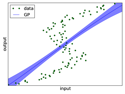
In our work, we want to present an algorithm that considers a number of problems in redshift regression that have been known to the community for a long time but have not been tackled and/or been ignored over the last decade. As it can be study in all plots showing the regressed redshift versus the actual redshift: the redshift regression problem is actually multimodal. This means that a given color can generally be explained by more than one redshift, cf. Fig. 1. In our work, we will also show that the RMS is an inadequate measure to estimate the accuracy of photometric redshift regression algorithms and present a more useful measure. This measure will be based on the posterior distribution over the redshift which should be rather considered in a multimodal problem. Another striking problem of the existing methodology is, that the uncertainty of the input data can not be considered so far, i.e. that uncertainties, or even more drastic missing values, of the colors can not be considered. Despite that, it has been claimed, that these regression algorithms can be used for predicting out-of-sample (i.e., higher redshifts than provided by the training) regression values. While in practice this might be possible, it is conceptually highly questionable whether this is the right concept. Instead we can provide with the model-based approach an alternative in the search for highly-redshifted extra-galactic objects, however, a lot more work has to be done in order to achieve this goal.

Figure 1: Example of a multimodal problem. It is evident that the Gaussian process is not capable of describing the multimodal data accordingly.

We start with a description of the data used in Section 2, followed by a description of the methodology in Section 3. In the following part the results are presented which contains also a direct comparison with the random forest. Subsequently, we summarize in Section 5 the work and show potential prospects for continuing the presented work.

2 Data

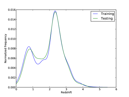
The presented methodology is conceptually new and is very different from the approaches used in the literature of photometric redshift regression. For this reason, we demonstrate our methodology on a small subset of quasars contained in the BOSS catalog. First, we extract 7506 randomly selected quasar spectra from BOSS which we divide into a training (5000) and test set (2506), the redshift distributions can be seen in Figure2. The idea is now to extract the photometry directly from the spectra instead of using their observed direct photometric counterparts. This way of approaching the problem has many advantages:

• no calibration of the zero points needed

• no uncertainties in the observables (spectra are considered noiseless)

• full control over how data have been generated

One of the downsides of using the spectra is that not the entire $u$ band is covered and thus we just have 3 colors to our availability (in the presented case these will be the three independent colors $g-r$, $g-i$, $g-z$). Note that in our methodology the fluxes themselves are used instead of colours and therefore the data presented to our algorithm are four dimensional. This is not an advantage as our model contains an additional scaling that has to be optimized.

Figure 2: Redshift distribution of training and test data.

Preprocessing

All the required spectra are downloaded from the SDSS server.In a first step, all the spectra are binned with a binning factor of 10 according to the following rules:

$$\lambda^{j}_{new}=\frac{1}{10}\sum_{i=10j}^{10(j+1)}\lambda^{i}_{old}$$

$$f^{j}_{new}=\frac{\sum_{i=10j}^{10(j+1)}f^{i}_{old}(\Delta f^{i}_{old})^{-2}}{\sum_{i=10j}^{10(j+1)}(\Delta f^{i}_{old})^{-2}}$$

$$\Delta f^{j}_{new}=\frac{1}{\sum_{i=10j}^{10(j+1)}(\Delta f^{i}_{old})^{-2}}$$

where $\lambda$, $f$ and $\Delta f$ are the wavelength, the spectral flux and the error of the spectral flux respectively. Subsequently, the spectra are shifted into their restframe and the flux values are extracted on a fixed grid ($\lambda\in[500,10400]$ in 1000 equally spaced steps) using spline interpolation. All missing parts are highlighted by an infinite flux and an infinite error on the flux.

3 Methodology

3.1 Uncertain PCA

3.2 Redshift regression model

In the previous section, a detailed description of the principle of the PCA, fed with uncertain spectra, was given. This PCA provides us now with a tool that can generate any kind of observed spectrum, simply based on the low-dimensional coordinates. In order to convert this into a redshift regression model, we assume the following things: With the PCA-weights $W\in\mathcal{R}^{LxD}$ and given coordinates $\theta\in\mathcal{R}^{1xL}$ we obtain a spectrum $\mathcal{S}=\theta\cdot W\in\mathcal{R}$, with $\cdot$ denoting the dot product. In general, this spectrum is not necessarily at a redshift of $z=0$, and thus the spectrum would be a function of $\mathcal{S}(\theta,z)$. Finally we are observing photometric magnitudes and therefore, we have to integrate the obtained spectrum over the filter curve of a filter $b$. The flux $\mathcal{I}$ in a band b is thus computed as

$$\mathcal{I}_{b}(\theta,z)=\frac{\int_{0}^{\infty}\lambda S(\lambda/(z+1))f_{b}(\lambda)d\lambda}{\int_{0}^{\infty}\lambda f_{b}(\lambda)d\lambda}.$$

Since the spectra are discrete the transformation $S(\lambda/(z+1))$ is not helpful for calculating the gradient with respect to $z$. That is why, we use the replacement

$$\tilde{\lambda}=\lambda/(z+1)$$

$$\frac{d\tilde{\lambda}}{d\lambda}=1/(z+1)\Rightarrow d{\lambda}=(z+1)d\tilde{\lambda}$$

and thus

$$\begin{split}\mathcal{I}_{b}(S,z)&=\frac{\int_{0}^{\infty}(z+1)\tilde{\lambda}S(\tilde{\lambda})f_{b}((z+1)\tilde{\lambda})(z+1)d\tilde{\lambda}}{\int_{0}^{\infty}(z+1)\tilde{\lambda}f_{b}((z+1)\tilde{\lambda})(z+1)d\tilde{\lambda}}\\ &=\frac{\int_{0}^{\infty}\lambda S(\lambda)f_{b}((z+1)\lambda)d\lambda}{\int_{0}^{\infty}\lambda f_{b}((z+1)\lambda)d\lambda}.\\ \end{split}$$ (1)

Effectively, we have now pushed the redshift from the discontinuous spectrum to the discontinuous filter bands by replacing $\tilde{\lambda}\rightarrow\lambda$. However, these can be easily approximated with an analytical function, here with a mixture of Gaussians

$$f(\lambda)=\sum_{c=1}^{N_{comp}}V_{c}\exp\left(-0.5\left(\frac{\mu_{c}-\lambda}{\sigma_{c}}\right)^{2}\right)$$

with $V_{c}$,$\mu_{c}$,$\sigma_{c}$ being the weights, the means and the widths of each of the $N_{comp}$ Gaussian components.

In order to compute now the expected flux from our model, we can approximate this integral with a regular Riemann sum, where the bin width $\Delta$ is given by the distance between two regularly sampled grid points, as described in the preprocessing. Finally, the flux in band $b$ is computed as

$$\begin{split}\mathcal{I}_{b}(\theta,z)&\approx\frac{\Delta\sum^{D}_{d}\lambda_{d}\theta\cdot W(\lambda_{d})f_{b}((z+1)\lambda_{d})}{\Delta\sum^{D}_{d}\lambda_{d}f_{b}((z+1)\lambda_{d}})\\ &=\frac{\sum^{D}_{d}\lambda_{d}\theta\cdot W(\lambda_{d})f_{b}((z+1)\lambda_{d})}{\sum^{D}_{d}\lambda_{d}f_{b}((z+1)\lambda_{d})}.\\ \end{split}$$ (2)

In summary, we know how the flux in a band $b$ for a spectrum defined by PCA coordinates $\theta$, redshift $z$ can be computed. Now, all we have to do is to convert the observed magnitudes to equivalent fluxes in the spectra.

Lastly, an arbitrary scaling constant $s$ has to be introduced, in order to accomodate for the difference in average flux and thus the full loss function $\mathcal{L}$ reads

$$\mathcal{L}\left(\theta,z,s\right)=\sum_{b}\left(\frac{s\mathcal{I}_{b}\left(\theta,z\right)-10^{-0.4(T_{b}-ZP_{b})}}{\sigma_{b}}\right)^{2}$$ (3)

where $T_{b}$ and $\sigma_{b}$ are the magnitudes and their respective uncertainties of the object observed in band $b$. For this objective loss function, the gradient with respect to $s$, $\theta$ and $z$ are computed and the loss is optimized using conjugate gradient (CG).

In experiments we learned that even a PCA with just 10 principle components leads to severe over-fitting of the likelihood function. For this reason, the optimizer converges to the closest local minimum (which due to the over-fitting is one of many local minima) during the non-convex optimization of the redshift. It is quite estonishing to see that a 10-dimensional linear model can lead to such behaviour but it seems that the broad integration over the filters washes out too many details which can be imitated by the PCA. The models that are fitted are usually unphysical since the models allowed by the PCA are not necessarily supported by data. In order to counteract this problem, we could either constrain the coordinates in the lower-dimensional space to the regions supported by actual data or draw prototypes from the projected data. As the former method would require even more assumptions about flexibility of the model, we decided to draw prototypes instead. Apart from imputing less assumptions, that puts us into the situation to evaluate redshifts in a fully Bayesian framework.

To that end all the parameters from the model are evaluated on a grid, see e.g. Tab. 1. For the scaling we assume an uninformative prior

$$Pr(s)=\frac{1}{\log s_{max}-\log s_{min}}\frac{1}{s}$$

while for the redshift and the prototypes a uniform prior is assumed respectively. Finally, we can compute the posterior of the model, given data, over $z$ as

$$P(z)=\frac{\sum_{s}\sum_{p}\exp{\left(-0.5\mathcal{L}\left(p,z,s\right)\right)}Pr(z)Pr(s)}{\sum_{z}\sum_{s}\sum_{p}\exp\left(-0.5\mathcal{L}\left(p,z,s\right)\right)Pr(z)Pr(s)}.$$ (4)

With the computation of this posterior we can achieve multiple things. First of all, the model is aware of the multi-modality of the problem, i.e., with the given data we obtain an a posteriori density of an arbitrary shape. In the results section, we will show how this can be effectively used to estimate redshifts and compare this to classical regression algorithms like the random forest. Secondly, we have now the choice to select a prior on $z$. In the given task, we chose an uninformed prior (uniform). This is in strong contrast to the machine learning architecture usually applied in this case. There, the bias which is inherent in the training is automatically propagated to the predictions as well. While this might be of advantage in some cases, it is a generally unwanted side-effect of the training procedure. In section XX we will explicitly make use of this advantage and show that the detection of high-redshifted quasars is more favorable in an unbiased setting.

parameter	grid	grid points
scaling	0.5:2.0:0.025	60
prototypes	1:5000:1	5000
redshifts	0:5.5:0.025	220

Table 1: Evaluation parameters for the Bayesian framework

3.3 Application of the algorithms

We apply our method on the 2506 training objects, where the templates are the 5000 PCA reconstructed training spectra. The dimensionality of the PCA embedding is (arbitrarily) set to 10. In order to calculate the posterior distribution according to Eq. 4 we need to choose the variances ${\sigma_{b}}^{2}$ for all the bands $b$. In principle this error is dominated by the uncertainty of the photometric measurements, however in the presented work, we artifically created them by integrating the raw spectra and thus no uncertainty enters the photometry. Still we see a deviation between the real spectra and the recovered ones which is due to the imperfect reconstruction of the spectra using the PCA. So in this case we use the training set to estimate the standard deviation for each band by comparing the magnitude obtained from the real and the reconstructed spectrum.

The mode prediction $z_{mode}$ is computed by finding the maximum of the posterior distribution

$$z_{mode}=\operatorname*{\arg\!\max}\limits_{z}(P(z)).$$

These mode values are then considered the predictions of our regression model from which the $MAD$ and the $STD$ are computed.

The random forest (Breiman, 2001) is trained on the 5000 training objects and used for prediction on the test values. The number of trees is set to 1000, even though the data are just three dimensional. In order to convert the point predictions of the random forest into a probability density, we assume that the predictions made by the random forest $z_{RF}$ are actually normally distributed as $P(z)=\mathcal{N}\left(z|z_{RF},\sigma^{2}\right)$. Consequently, we have to determine a value for $\sigma$. The most intuitive way is to compare actual and predicted values for the training dataset, leading to $\sigma=0.30$. Alternatively, $\sigma$ can be chosen such that $\frac{1}{N}$logL_True is optimized ($\sigma=0.76$). However, it should be noted, that this is not a practical way of optimization, as by definition test data should not be used for the optimization of model parameters. Here, this is just done for convenience to show that even a very uncertain prediction can not outperform the presented algorithm.

The Gaussian process (Rasmussen & Williams, 2005) is chosen as a regression model, as it provides immediatelly a (normal) distribution of the output values. Therefore, these mean predictions and their variances can be directly used to calculate $\frac{1}{N}$logL_True and $\langle KLD\rangle$.

4 Results

4.1 Validation

A common measure to compare the performance of the redshift regression algorithms is to use the root mean square (RMS) on the normalized redshift deviation

$$\Delta z_{norm}=\frac{z_{reg}-z_{true}}{1+z_{true}}.$$

Here, we use for convience the standard deviation (STD) which is for $N=2506$ this is also equivalent to the RMS. Another frequently used measure is the median absolute deviation (MAD) as this is less susceptible to objects deviating extremely from the locus.

With the example in the introduction we could, however, convincingly show that these measures are rather meaningless in the setting of a multimodal model as the optimization for the mean behaviour produces misleading predictions. For this reason, we propose two new measure that are capable to take into account the multimodality of the regression value. Since our model returns a posterior distribution over $z$, we might ask how probable the true redshift $z_{true}$ is according to our model and thus we can compute

$$\frac{1}{N}\mathrm{logL}_{\mathrm{True}}=\frac{1}{N_{test}}\sum_{n=1}^{N_{test}}P_{n}\left(z_{n;\,true}\right)$$ (5)

where $N_{test}=2506$ is the number test items.

Another measure which tells us whether we captured the multi-modality of the data correctly is to investigate what other redshifts originate from similar colors. For this reason, we perform a $k$ nearest neighbour search in the colour space and identify the closest $k$ redshifts from the training data. In this case, we chose $k=10$ but the statement also holds for other values of $k$. On these 10 redshifts we perform a kernel density estimation (KDE) and can conequently compute the Kullback-Leibler-divergence between the neighboring redshifts $K(z)$, computed from the KDE and the posterior $P(z)$ as

$$\begin{split}KLD(K,P)&=\int K(z)\log{\frac{K(z)}{P(z)}}dz\\ &\approx\frac{1}{k}\sum_{k^{\prime}=1}^{k}\log{K\left(z_{k^{\prime}}\right)}-\log{P\left(z_{k^{\prime}}\right)}\\ \end{split}$$

This is done for all $N_{test}$ objects and the average

$$\langle KLD\rangle=\frac{1}{N_{test}}\sum_{n=1}^{N_{test}}KLD_{n}$$ (6)

over them is used. The KLD tells us how dissimilar the two distributions are and thus lower values indicate a better agreement.

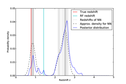
At this point the question might arise, why we should not use the $k$ nearest neighbours ($k$NN) approach to model the posterior density. Inarguably, this would provide us with a sampled version of the true posterior distribution, but to actually model the point estimates as a distribution, a density estimator would have to be quantified. These can estimate the underlying density more accurately the higher $k$ is chosen, however, it has to be validated what a meaningful value for $k$ is. Therefore, this method would again depend on several free parameters which may alter the appearence of the distribution accordingly. In addition, this would again be a data-driven approach which is neither capable of including the uncertainties of the colors nor allows for predictions outside the training sample. For this reason, it is only used for cross-validating our developed model and to verify that our obtained distribution is similar to the true underlying one. In Fig. 3 an illustrative example is shown. The red line denotes the actual redshift of the object, the cyan one the prediction by the random forest. The gray lines are the redshifts of 20 nearest neighbours in color space. This distribution is modeled using kernel density estimation and returns the dashed black curve. Finally, the blue curve is the posterior distribution as obtained by our model . Clearly, a very similar behaviour is observed, strenghtening the principle idea of our model.

Figure 3: For a given data item the actual (spectroscopic) redshift is shown in red. The redshift obtained by random forest regression (or kNN regression) is shown in magenta. In addition, the redshifts of the nearest neighbor objects in terms of the colour space are shown in transparent black, vertical lines. This density is then approximated by a Kernel density estimation (KDE) and compared to the posterior distribution of the presented model.

4.2 Comparison of the algorithms

In Tab. 2, the result for the described experiment is shown. For the commonly used $STD$, we can see that the GP and RF perform comparably well and significantly better than our presented algorithm. However, for all remaining measures the presented algorithm performs drastically better than the compared algorithms.

	Here	RF	RF	GP
		($\sigma=0.30$)	($\sigma=0.76$)
$STD$	0.476	0.344	0.344	0.326
$MAD$	0.078	0.123	0.123	0.111
$\frac{1}{N}$logLTrue	-0.514	-2.979	-1.138	-77.875
$\langle KLD\rangle$	1.082	3.491	1.536	81.660

Table 2: Summary of the results for the presented toy example.

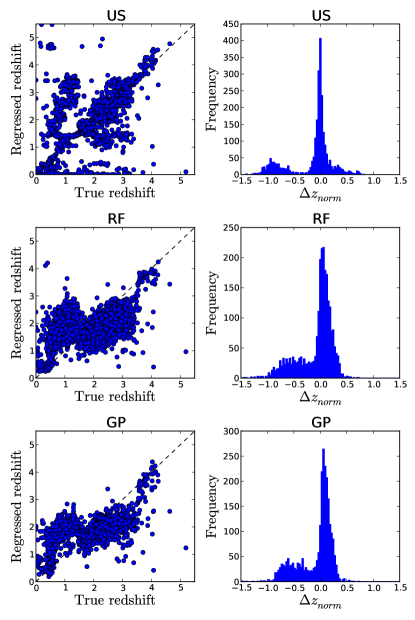
In order to understand the results, we have to understand the difference between the measures presented. In Fig. 4, the regressed redshift is plotted against the true one and additionally a histogram over $\Delta z_{norm}$ is shown for each of the algorithms. On a first look, we can clearly see, why the $STD$ is much worse for the algorithm presented in this work. While for the GP and RF the points are all distributed along the line, there are some very drastic deviations apparent in our algorithm. This behaviour is actually a bias in the training dataset which for the GP and RF is propagated through the algorithm, while in our case it is omitted. Since most training redshift are located between $[2,3]$ (cf., Fig 2), predictions of objects that are not very certain will by design between $[2,3]$ as well. This is reasonable, if the redshift distribution is similar for training in testing. If this can not be guaranteed (as in most realistic settings, since the observational biases between surveys can be different), this will effectively lead to an amplification of this bias and thus even worse predictions will be produced, as shown later on. In our model, all redshifts are equally likely (uniform prior), but of course we can influence this behaviour by telling our prior about the distributions of redshifts. If we do so, the predictions are, by design, much more constraint towards a straight line, which is also reflected in significantly lower $STD$ of 0.400.

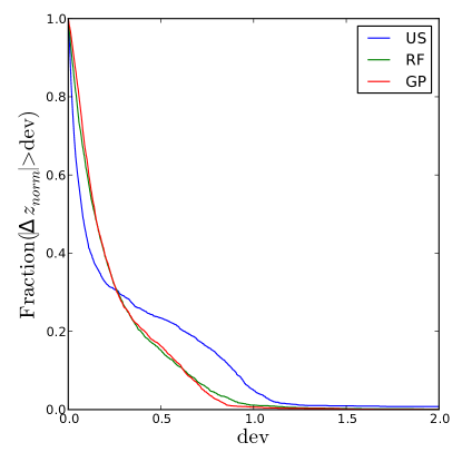
The $MAD$ behaves differently as for this heavily deviating objects are only marginally considered. As a consequence, the $MAD$ measures rather the width of the central distribution than the width of the full distribution. As evident from Fig. 4, the predictions obtained from our model are much more precise than the ones by the RF or GP. This becomes even clearer if we consider the fraction of objects that deviate more than a certain value, cf. Fig. 5. For the vast majority of the objects ($\approx 70\%$) the deviation from the true value is considerably lower than for the RF and GP predictions. The higher precision originates from the superior knowledge provided to the model-based algorithm which can describe the behaviour of the spectra in more detail than the data-driven approaches ever could.

As stated in the former sections, it is questionable why for a multimodal problem the average prediction should be considered, as this leads necassarily to wrong prediction. Instead, it should be considered how well the obtained distributions reflect the underlying multimodality of the model. For this reason we measure the averaged likelihood that each of the models can explain the true redshift of a given item. If we just consider the RF optimized on training data ($\sigma=0.3$), the Bayes factor ($\approx 11.8$) provides strong evidence that our model is better supported by the provided data. In addition, we can also see that the average $KLD$ is by more than a factor of three smaller than the one by the random forest, supporting the power of the presented algorithm. In both cases, the GP does not even come to comparable values as the individual predictions for the GP are appearently over-certain as compared to their true nature.

Figure 4: Each row shows the results of the experiment noted on top of each plot (our algorithm, random forest and Gaussian process). On the left side the value obtained by the regression algorithm is plotted against the actual value. On the right one can see a histogram of $\Delta z_{norm}=\frac{z_{reg}-z_{true}}{1+z_{true}}$. One can clearly see that for our presented method the peak is much sharper, but the left wing is much more pronounced than for the other two algorithms.

Figure 5: The fraction of objects deviating with more than $|\Delta z_{norm}|>dev$ is plotted. While the random forest and the Gaussian process show a very similar behaviour, our presented algorithm can predict the redshift for 60% of the objects significantly more precise but is heavily influenced from redshifts deviating more than 0.3.

5 Discussion

In this work, we presented an alternative way of modeling photometric redshifts. The idea was to combine the advantages of model-based approaches (full model control, Bayesian framework, multimodality) with the ones from the data-driven approaches (no explicit model-formulation). For this reason a probabilistic PCA was developed which can produce projections in the presence of missing and uncertain data. In a first step, we tried to utilize this projection to optimize for the coordinates of the PCA, but learned that if the coordinates are unconstrained already a 10-dimensional PCA can produce unphysical spectra which then lead to overfitting. Instead, we used the provided reconstructed spectra themselves as prototypes and therefore converted the continuous model into a discrete one. With these prototypes at hand, we were able to treat the regression problem in a fully Bayesian framework which allowed us to compute the posterior distribution over the redshift.

We compared the distribution of our model with predictions made by the random forest and the Gaussian process. Even though, we emphasize that this comparison is fairly meaningless as the different approaches are tailored for different tasks. The standard regression models (RF, GP) are capable of describing a function-like behaviour (one input maps to a redshift), while it is long known that the photometric redshift regression problem is a multimodal one (one input can map to several redshifts). Therefore, also the measure of the $RMS$ and the $MAD$, as commonly done in the literature, are questionable measures of the quality of a regression algorithm. For this reason, we introduced two additional measures which reflect the likelihood of capturing the true underlying redshift and on the other hand a measure denoting how well we can describe similar colors with different redshifts. By design, our presented algorithm is capable of describing this behaviour, while the standard regression models are not, as they expect a one-to-one (or many-to-one) mapping. We would like to highlight, that the choice of the methodology is only of minor importance, as long as the wrong objective is measured. To treat this multimodality purely with data-driven methodology is quite complicated, even though, some approaches already exist (e.g., mixture density networks). Consequently, past publications have utilized a measured that simply not adequate for the task at hand.

Prospects

The presented approach can be developed further in two aspects: the methodological one and the astronomical one. The biggest disadvantage of the current design is, that rather prototypes are extracted and used for prediction than a continuous PCA model. The problem of the continuous PCA model is its high flexibility which leads to severe overfitting. For this reason, it would be desirable to constrain the PCA in the lower dimensional space by, for example, estimating the density of the spectra. This density estimate could then be used as a prior weighting the frequency of the a PCA coordinate in the real spectra. In case that this density can be written as a mixture of Gaussians, it might be even possible to marginalize the posterior over the PCA coordinates analytically. This would make the model extremely fast and would omit the point of sampling or drawing prototypes.

From an astronomical point of view, more work has to be done. So far we have just provided the functioning on a small toy dataset where the magnitudes were extracted with the provided filter curves and (known and noise-free) zero points were added. We chose this setting, as we wanted to have full control on the model and not to be distracted by errorneous and noisy calibrations. It is important to notice that a purely data-driven approach can deal with this quite naturally, while the presented algorithm depends heavily on the correctness of these calibrations. On the other hand, it is of course also possible to include a given uncertainty of the zero points into the model and also this can be cross-validated using a training set. In summary, a much more detailed understanding of how photometric measurements relate to the spectra is required.

Another striking advantage of our model is, that we can include uncertainty of the photometric measurements directly into the model. This includes also missing values which are a common struggle in astronomy due to the different coverage and depth of the surveys. This is contrast to nearly all data-driven algorithms which can at maximum handle the input uncertainty by sampling (which is hard for a missing value).

A different prospect of our model would be to extent the PCA model towards the infrared. At the moment, our coverage above $1\mu m$ is very shallow and thus it would be desirable to retrieve near-infrared to mid-infrared spectra of low-redshifted quasars (as otherwise the rest-frame would be in the optical again). This would allow us to include also infrared data as then the coverage of the prototypes would reach into the near infrared. It is important to notice that it does not matter whether the infrared spectra are the same objects as the optical ones, it only has to be guaranteed that there is considerable overlap with the prototypes as they are now.

References

- Abdalla et al. (2008) Abdalla F. B., Amara A., Capak P., Cypriano E. S., Lahav O., Rhodes J., 2008, MNRAS, 387, 969
- Antonucci (1993) Antonucci R., 1993, ARA&A, 31, 473
- Arnalte-Mur et al. (2010) Arnalte-Mur P., Fernández-Soto A., Martínez V. J., Saar E., 2010, 14, 255
- Bolzonella et al. (2000) Bolzonella M., Miralles J.-M., Pelló R., 2000, AAp, 363, 476
- Breiman (2001) Breiman L., 2001, Mach. Learn., 45, 5
- Laurino et al. (2011) Laurino O., D’Abrusco R., Longo G., Riccio G., 2011, MNRAS, 418, 2165
- O’Mill et al. (2011) O’Mill A. L., Duplancic F., García Lambas D., Sodré Jr. L., 2011, MNRAS, 413, 1395
- Rasmussen & Williams (2005) Rasmussen C. E., Williams C. K. I., 2005, Gaussian Processes for Machine Learning (Adaptive Computation and Machine Learning). The MIT Press
- Subbarao et al. (1996) Subbarao M. U., Connolly A. J., Szalay A. S., Koo D. C., 1996, AJ, 112, 929
- Wu & Jia (2010) Wu X.-B., Jia Z., 2010, MNRAS, 406, 1583