Heralding pure single photons: a comparision between counter-propagating and co-propagating twin photons.

Abstract

We investigate the possibility of generating pure heralded single photons through spontaneous parametric down-conversion comparing the counter-propagating geometry studied in Gatti et al. (2015) with more conventional co-propagating configurations which enhance the purity of the heralded photon state through the technique of group-velocity matching. We estimate the Schmidt number associated to the temporal modes as a function of the pump pulse duration for three particular configurations, showing how the different phase-matching conditions influences the degree of separability that can be achieved.

Introduction

In the process of spontaneous parametric down-conversion (SPDC) occurring in a $\chi^{(2)}$ material, photons belonging to the laser pump field are split into pairs of photons of lower energies and momentum. The generated photon pairs, are naturally entangled in a number of variables (energy, momentum, angular momentum, polarization) as a consequence of the conservation laws ruling the microscopic process. Because of its relative simplicity of implementation, SPDC is indeed a widely used source of entangled light. At the same time, it is also the most frequently used source of pure photons heralded by the detection of their twin partner, the starting point of many quantum information protocols. In this latter case entanglement must be avoided as much as possible, since the heralded photons are required to be in indistinguishable and capable of high-visibility interference. Filtering is the simplest method for achieving this purpose, through it presents the drawback of drastically reducing the efficiency of the source In order to achieve pure heralded photons with high fluxes, considerable effort has been devoted to find alternative techniques that do not rely on post-selection Grice et al. (2001); U’Ren et al. (2006); Mosley et al. (2008a); Migdall et al. (2002); Levine et al. (2010); Bennink (2010); Brańczyk et al. (2011); Zhang et al. (2012). They consist in manipulating directly the degree of entanglement of the source by controlling the modal structure of the emitted photon pairs in order to produce uncorrelated twin photons In such a way a conditioned measurement projects the field in a pure single photon state rather than in a mixed state, and pure heralded photon can be obtained without filtering. A recent survey of these techniques can be found in Migdall et al. (2013).

In this work we investigate different configuration to eliminate entanglement in the temporal frequency domain, in particular comparing a co-propagating and a counter-propagating geometry. In the latter, proposed by Harris in the sixties Harris (1966) and implemented in 2007 by Canalias et al. Canalias and Pasiskevicius (2007), twin photons are emitted along opposite directions in a periodically poled crystal with a submicrometric poling period. The technological challenges involved in the fabrication of crystals with such a short poling period are described e.g. in Canalias et al. (2003); Pasiskevicius et al. (2012). With respect to the standard co-propagating configuration where the twin photons are typically emitted over a broad range of frequencies, counter-propagating photons have much narrower spectral bandwidths imposed by the peculiar phase-matching conditions characterizing this geometry Strömqvist et al. (2012); Suhara and Ohno (2010); Gatti et al. (2015); Corti et al. (2016). Because of this feature, the counter-propagating SPDC configuration has soon been recognized as a promising source for generating heralded single photons Christ et al. (2009); Gatti et al. (2015). A detailed analysis of the temporal coherence and correlation of counter-propagating twin photons and twin beams has been performed in previous works of ours Gatti et al. (2015); Corti et al. (2016) , where we studied both the spontaneous regime Gatti et al. (2015) and the stimulated regime of photon pair production Corti et al. (2016).

In this work we focus on the purely spontaneous regime, where the system can be exploited as a source of heralded single photons, and we provide a detailed comparison between this source and the conventional co-propagating configuration. In the latter case, a separable two-photon state can be achieved only through the techniques of group velocity matching, which require a careful choice of the material and of the tuning conditions as well as sub-picosecond pump pulses Grice et al. (2001). Conversely, our analysis will show that in the counter-propagating geometry there is no need of such a fine tuning, and that highly monochromatic single photons in a pure state can be generated in a wide range of phase-matching conditions and pump durations. Conversely, our analysis will show that in the counterpropagating geometry there is no need of such a fine tuning, and that highly monochromatic single photons in a pure state can be generated in a wide range of phase-matching conditions and pump durations. In particular, we shall emphasize how the different time scales in play characterizing the two configurations strongly affect the conditions in which separability can be achieved and are at the origin of the different behaviors of the two sources.

The paper is organized as follows: Sec.I illustrates the two geometries and their different phase-matching conditions. Sec.II evaluates the degree of entanglement of the two-photon state, providing approximated analytical expressions for the Schmidt number, valid in both geometries. Examples of specific configurations suitable for generating pure heralded photons are analyzed in Sec.III and compared with the counter-propagating geometry. The spectral properties of co-propagating and counterpropagating twin photons are finally analysed in Sec. IV.

I Phase-matching in the counter- and co-propagating geometries

We restrict our analysis to a purely temporal description: we consider only collinear propagation, either assuming that a small angular bandwidth is collected and the process is characterized by a single spatial mode operation, or because of a waveguiding configuration.

We first consider the counter-propagating geometry shown in Fig.1a, with a coherent pump pulse of central frequency $\omega_{p}$ and temporal profile $\alpha_{p}(t)$ impinging a periodically poled crystal of length $l_{c}$ from the left face and generating counter-propagating photon pairs with, say, the idler photon propagating opposite to the pump.

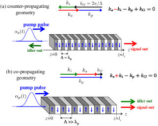
Figure 1: (a) Scheme of twin-photon generation in the (a) counter-propagating and (b) co-propagating geometries. In case (a) the quasi-phasematching for collinear propagation requires a submicrometric poling period, $k_{G}\sim k_{p}$, while the co-propagating process (b) can be phase matched either in bulk crystals, or with larger poling periods $\Lambda$ .

This occurs when the poling period $\Lambda$ is on the same order of the pump wavelength in the medium $\lambda_{p}/n_{p}$: in this case the first-order momentum associated to the nonlinear grating, $k_{G}=2\pi/\Lambda$ is able to compensate the pump photon momentum so that twin photons must be emitted along opposite directions in order to satisfy momentum conservation (Fig.1a). The central frequencies of the emitted signal and idler fields, $\omega_{s}$ and $\omega_{i}=\omega_{p}-\omega_{s}$, are thus determined by the crystal poling period $\Lambda$ and the pump central frequency $\omega_{p}$ according to the following quasi-phasematching condition

$$k_{s}-k_{i}=k_{p}-k_{G}\;\;\text{\small{{\bf(a) counter-propagating case}}}$$ (1)

where $k_{j}:=\frac{\omega_{j}}{c}n_{j}(\omega_{j})$, $j=s,i,p$ denotes the wave-number at the corresponding central frequencies $\omega_{j}$.

For comparison, we shall also consider the more common co-propagating geometry (Fig.1b) where the all the three fields propagate along the positive $z$ direction. In this case the wave-numbers at the reference frequencies satisfy the following condition

$$k_{s}+k_{i}=k_{p}-k_{G}\;\;\text{\small{{\bf(b) co-propagating case}}}$$ (2)

which can describe both the case of a bulk crystal, in which $k_{G}=0$, or quasi-phasematching in periodically poled structures with $k_{G}\ll k_{j}$, $j=i,s,p$.

Considering the regime of photon-pair production, the generated two photon state conditioned by a photon count has the form Gatti et al. (2015)

$$|\phi_{\mathrm{C}}\rangle=\int d\Omega_{s}d\Omega_{i}\psi(\Omega_{s},\Omega_{i})\hat{a}_{s}^{\dagger}(\Omega_{s})\hat{a}_{i}^{\dagger}(\Omega_{i})\left|0\right\rangle$$ (3)

where $\hat{a}_{s}^{\dagger}(\Omega_{s})$ and $\hat{a}_{i}^{\dagger}(\Omega_{i})$ denote the signal and idler creation operators in the frequency domain ($\Omega_{j}$ is the offset from the reference frequency $\omega_{j}$), and

$$\psi(\Omega_{s},\Omega_{i})=\frac{g}{\sqrt{2\pi}}\tilde{\alpha}_{p}(\Omega_{s}+\Omega_{i})$$

$$\times e^{-i\frac{1}{2}{\cal D}^{\text{\tiny{$(l)$}}}(\Omega_{s},\Omega_{i})l_{c}}{\rm sinc}\left[\frac{{\cal D}^{\text{\tiny{$(l)$}}}(\Omega_{s},\Omega_{i})l_{c}}{2}\right],\;\;(i=a,b)$$ (4)

is the so-called biphoton amplitude, giving the joint probability amplitude of detecting a signal photon at frequency $\omega_{s}+\Omega_{s}$ and an idler photon at frequency $\omega_{i}+\Omega_{i}$. Here, ${\cal D}^{\text{\tiny{$(l)$}}}(\Omega_{s},\Omega_{i})l_{c}$ denote the phase-mismatch functions, where the $i=a,b$ superscripts refer to the counter-propagating and the co-propagating configuration respectively. $\tilde{\alpha}_{p}(\Omega)$ is the spectral amplitude of the pump pulse normalized by its peak value

$$\tilde{\alpha}_{p}(\Omega)=\int\frac{dt}{\sqrt{2\pi}}e^{i\Omega t}\frac{\alpha_{p}(t)}{\alpha_{p}(t=0)}\,,$$ (5)

The differences between the two geometries arise because of the different sign characterizing the two phase-mismatch functions

$${\cal D}^{\text{\tiny{$(l)$}}}(\Omega_{s},\Omega_{i})$$

$$=\left\{\begin{array}[]{lr}k_{s}(\Omega_{s})-k_{i}(\Omega_{s})-k_{p}(\Omega_{s}+\Omega_{i})+k_{G},&\text{ $l=a$}\\ k_{s}(\Omega_{s})+k_{i}(\Omega_{s})-k_{p}(\Omega_{s}+\Omega_{i})+k_{G},&\text{ $l=b$}\end{array}\right.$$ (8)

As extensively described in Gatti et al. (2015); Corti et al. (2016), the properties of the counter-propagating twin photons strongly differ from those of the co-propagating ones, because of the minus sign in front of the idler wave-number $k_{i}(\Omega_{i})$. This is best seen by expanding the phase mismatch (8) at first order around the reference frequencies (corresponding to $\Omega_{j}=0$), obtaining thereby

$$\frac{1}{2}{\cal D}^{\text{\tiny{$(l)$}}}(\Omega_{s},\Omega_{i})l_{c} \approx \frac{l_{c}}{2}[(k_{s}^{\prime}-k_{p}^{\prime})\Omega_{s}-(k_{p}^{\prime}\mp k_{i}^{\prime})\Omega_{i}]$$ (9)

$$\equiv -\left({\tau_{p,s}^{\text{\tiny{($-$)}}}}\Omega_{s}+{\tau_{p,i}^{\text{\tiny{($\pm$)}}}}\Omega_{i}\right)\;,$$ (10)

where the $+$ and $-$ minus sign refer to the counter-propagating $(l=a)$ and co-propagating $(l=b)$ cases, respectively, $k_{j}^{\prime}\equiv v_{gj}^{-1}=\left(\frac{dk_{j}}{d\Omega_{j}}\right)_{\Omega_{j}=0}$ is the inverse group velocity of wave $j$ at its reference frequency $\omega_{j}$ and the characteristic times

$${\tau_{j}^{\text{\tiny{($\pm$)}}}}=\frac{1}{2}\left(\frac{l_{c}}{v_{gp}}\pm\frac{l_{c}}{v_{gj}}\right)\;\;\;j=i,s$$ (11)

involve either the difference or the sum of the inverse group velocities of the pump and of the wave $j=i,s$, depending whether the latter copropagates or counterpropagates with respect to the former. The omission of higher order dispersion terms is justified in the counter-propagating configuration, which typically involves narrow down-conversion spectra Canalias and Pasiskevicius (2007); Gatti et al. (2015); Corti et al. (2016). In order to perform analytical calculations, we shall use the linear approximation (10) also for the co-propagating configuration, through in this case the effect of group velocity dispersion can be more relevant because of the larger bandwidths in play.

As discussed in Grice et al. (2001); U’Ren et al. (2006); Evans et al. (2010); Gatti et al. (2015), the possibility to generate heralded photons with a high degree of purity depends both on the relative sizes and signs of the time constants ${\tau_{p,s}^{\text{\tiny{($-$)}}}}$and ${\tau_{p,i}^{\text{\tiny{($\pm$)}}}}$ defined in Eq.(11), and on how they compare to the pump duration $\tau_{p}$ (notice that only ${\tau_{p,i}^{\text{\tiny{($+$)}}}}$ is always positive, while ${\tau_{p,s}^{\text{\tiny{($-$)}}}}$ and ${\tau_{p,i}^{\text{\tiny{($-$)}}}}$ can be either positive or negative). In the co-propagating geometry the two scales ${\tau_{p,s}^{\text{\tiny{($-$)}}}}$ and ${\tau_{p,i}^{\text{\tiny{($-$)}}}}$ are associated to the group velocity mismatch (GVM) of the signal and the idler with respect to the co-propagating pump. They are on the same order of magnitude, except for the particular case in which one of the two fields is velocity matched to the pump. By contrast, in the counter-propagating case, the time constant associated to the backward photon ${\tau_{p,i}^{\text{\tiny{($+$)}}}}=l_{c}/2v_{gp}+l_{c}/2v_{gi}$, which involves inverse group velocities sum (GVS), is on the order of the photon transit time across the crystal, and exceeds therefore the signal-pump GVM time ${\tau_{p,s}^{\text{\tiny{($-$)}}}}=l_{c}/2v_{gp}-l_{c}/2v_{gs}$ by at least an order of magnitude.

Therefore, considering the ratio between the two time constants ,

$$\eta={\tau_{p,s}^{\text{\tiny{($-$)}}}}/{\tau_{p,i}^{\text{\tiny{($\pm$)}}}}\;,$$ (12)

we have

$$|\eta|=\begin{cases}|{\tau_{p,s}^{\text{\tiny{($-$)}}}}|/|{\tau_{p,i}^{\text{\tiny{($+$)}}}}|\ll 1\;&\text{for case (a)}\\ |{\tau_{p,s}^{\text{\tiny{($-$)}}}}|/|{\tau_{p,i}^{\text{\tiny{($-$)}}}}|\;&\text{arbitrary for case (b)}.\end{cases}$$ (13)

Without loss of generality, in case (b) we shall assume that the signal and idler fields satisfy the condition $|{\tau_{p,s}^{\text{\tiny{($-$)}}}}|\leq|{\tau_{p,i}^{\text{\tiny{($-$)}}}}|$ so that in both configurations we have

$$-1\leq\eta\leq 1$$ (14)

II Entanglement quantification

We characterize the degree of entanglement with the Schmidt number Ekert and Knight (1995); Parker et al. (2000), which provides an estimate of the number modes participating to the entangled state van Exter et al. (2006). It is defined as the inverse of the purity of the state of each separate subsystem

$${\cal K}=\frac{1}{{\mathrm{T}r}\{\rho_{s}^{2}\}}=\frac{1}{{\mathrm{T}r}\{\rho_{i}^{2}\}}$$ (15)

where $\rho_{s}$, $\rho_{i}$ are the reduced density matrix of the signal and idler , e.g. $\rho_{s}={\mathrm{T}r}_{i}\{|\phi_{\mathrm{C}}\rangle\,\langle\phi_{\mathrm{C}}|\}$. For a biphoton state of the form (3), the Schmidt number can be expressed through integrals involving the first-order coherence functions of the signal and the idler fields

$$G_{s}^{(1)}(\Omega_{s},\Omega_{s}^{\prime})=\int d\Omega_{i}\psi^{*}(\Omega_{s},\Omega_{i})\psi(\Omega_{s}^{\prime},\Omega_{i})$$ (16)

$$G_{i}^{(1)}(\Omega_{i},\Omega_{i}^{\prime})=\int d\Omega_{i}\psi^{*}(\Omega_{s},\Omega_{i})\psi(\Omega_{s},\Omega_{i}^{\prime})$$ (17)

Namely, it is found that Gatti et al. (2012); Mikhailova et al. (2008)

$${\cal K}=\frac{{\cal N}^{2}}{B}$$ (18)

where

$${\cal N}= \int d\Omega\,G_{s}^{(1)}(\Omega,\Omega)=\int d\Omega\,G_{i}^{(1)}(\Omega,\Omega)$$ (19)

$$B= \int d\Omega\int d\Omega^{\prime}\left|G_{s}^{(1)}(\Omega,\Omega^{\prime})\right|^{2}$$

$$= \int d\Omega\int d\Omega^{\prime}\left|G_{i}^{(1)}(\Omega,\Omega^{\prime})\right|^{2}$$ (20)

In this work the Schmidt number ${\cal K}$ will be estimated by means of i) the numerical integration of Eqs.(18)-(20), where the phase-mismatch (8) is evaluated using the complete Sellmeier dispersion formula in Gurzadian et al. (1991); Kato and Takaoka (2002); Zernike (1964), or ii) a Gaussian approximation for the biphoton amplitude in Eq.(I), which is typically used in the literature Grice et al. (2001); Law and Eberly (2004); U’Ren et al. (2006). In the latter case, the sinc function in Eq.(I) is fitted by a Gaussian of its argument, setting

$${\rm sinc}\frac{{\cal D}^{\text{\tiny{$(l)$}}}(\Omega_{s},\Omega_{i})l_{c}}{2} \approx e^{-\gamma\left(\frac{{\cal D}^{\text{\tiny{$(l)$}}}(\Omega_{s},\Omega_{i})l_{c}}{2}\right)^{2}}$$ (21)

$$\approx e^{-\gamma\left({\tau_{p,s}^{\text{\tiny{($-$)}}}}\Omega_{s}+{\tau_{p,i}^{\text{\tiny{($\pm$)}}}}\Omega_{i}\right)^{2}}$$ (22)

where the linear approximation (9) of the phase mismatch has been used in the second line. $\gamma$ is a fitting parameter; e.g. requiring that the sinc and the Gaussian functions shares the same full width at half maximum (FWHM), one has $\gamma=0.193$. The approximation (22) allows to derive analytical results, which provide an immediate comparison between the various configurations, but neglects the effects of group velocity dispersion at second and higher orders.

Furthermore, we consider a pump pulse with a Gaussian temporal profile of duration $\tau_{p}$, $\alpha_{p}(t)=\alpha_{p}(0)e^{-t^{2}/2\tau_{p}^{2}}$ , so that the corresponding spectral amplitude (5) is given by

$$\tilde{\alpha}_{p}(\Omega)=\frac{1}{\Delta\Omega_{p}}e^{-\frac{\Omega_{p}^{2}}{2\Delta\Omega_{p}^{2}}},$$ (23)

where the spectral bandwidth is $\Delta\Omega_{p}=1/\tau_{p}$.
The biphoton amplitude (I) takes then the approximated form :

$$\psi(\Omega_{s},\Omega_{i})\approx \frac{g\tau_{p}}{\sqrt{2\pi}}e^{i\left[{\tau_{p,s}^{\text{\tiny{($-$)}}}}\Omega_{s}+{\tau_{p,i}^{\text{\tiny{($\pm$)}}}}\Omega_{i}\right]}$$ (24)

$$\times e^{-c_{11}\Omega_{s}^{2}-c_{22}\Omega_{i}^{2}-2c_{12}\Omega_{s}\Omega_{i}}$$

where the real coefficients $c_{ij}$ are

$$c_{11} = \frac{\tau_{p}^{2}}{2}+\gamma{\tau_{p,s}^{\text{\tiny{($-$)}}}}^{2},$$ (25)

$$c_{22} = \frac{\tau_{p}^{2}}{2}+\gamma{\tau_{p,i}^{\text{\tiny{($\pm$)}}}}^{2},$$ (26)

$$c_{12} = \frac{\tau_{p}^{2}}{2}+\gamma{\tau_{p,s}^{\text{\tiny{($-$)}}}}{\tau_{p,i}^{\text{\tiny{($\pm$)}}}}.$$ (27)

Here and in the following ${\tau_{p,i}^{\text{\tiny{($+$)}}}}$ refers to the counter-propagating case ($a$), ${\tau_{p,i}^{\text{\tiny{($-$)}}}}$ refers to co-propagating case ($b$). Inserting approximation (24) in the expression of ${\cal K}$ in Eqs.(18)-(20), we find

$${\cal K} =\sqrt{\frac{c_{11}c_{22}}{c_{11}c_{22}-c_{12}^{2}}}$$ (28)

$$=\frac{1}{1-\eta}\left[1+\eta^{2}+\frac{1}{2\gamma}\left(\frac{\tau_{p}}{{\tau_{p,i}^{\text{\tiny{($\pm$)}}}}}\right)^{2}+2\gamma\left(\frac{{\tau_{p,s}^{\text{\tiny{($-$)}}}}}{\tau_{p}}\right)^{2}\right]^{1/2}$$ (29)

As a function of the pump duration $\tau_{p}$, it is easily seen that ${\cal K}$ takes its minimum for

$$\tau_{p}^{min}=\sqrt{2\gamma|{\tau_{p,s}^{\text{\tiny{($-$)}}}}{\tau_{p,i}^{\text{\tiny{($\pm$)}}}}|}$$ (30)

The minimum value of ${\cal K}$ depends both on the sign and on the magnitude of $\eta$ and is given by

$${\cal K}_{min}=\left\{\begin{array}[]{ll}\frac{1+\eta}{1-\eta}&\text{for $\eta>0\rightarrow{\tau_{p,s}^{\text{\tiny{($-$)}}}}{\tau_{p,i}^{\text{\tiny{($\pm$)}}}}>0$}\\ 1&\text{for $\eta\leq 0\rightarrow{\tau_{p,s}^{\text{\tiny{($-$)}}}}{\tau_{p,i}^{\text{\tiny{($\pm$)}}}}\leq 0$}\end{array}\right.$$ (31)

Thus, within the validity of the Gaussian approximation (24), complete separability can be achieved only if $\eta\leq 0$. The condition $\eta=0$ corresponds to perfect velocity matching between the pump and the signal: ${\tau_{p,s}^{\text{\tiny{($-$)}}}}=0$. Notice that in this case perfect separability is reached only asymptotically for $\tau_{p}\to\tau_{p}^{min}=0$. Conversely, when $\eta<0$, perfect separability ${\cal K}=1$ can be in principle reached for finite pump durations, and requires that ${\tau_{p,s}^{\text{\tiny{($-$)}}}}$ and ${\tau_{p,i}^{\text{\tiny{($\pm$)}}}}$ have opposite signs. Once this condition is met, the mixed term coefficient (27) vanishes for a pump duration $\tau_{p}=\tau_{p}^{min}$.
Alternatively, for positive $\eta$, the two-photon state can be made almost separable by choosing a configuration for which $\eta$ is sufficiently small. Notice that this last condition is naturally fulfilled in the counter-propagating case.

III Specific configurations for separability

According to the results presented in Sec.II, we shall compare three distinct configurations which satisfy the conditions for complete or nearly complete separability:

(i) Counter-propagating geometry ($|\eta|<<1$)
The peculiarity of the counter-propagating geometry (a) is that the condition $|\eta|\ll 1$ is naturally fulfilled [see Eq.(13) and discussion]. Even for $\eta>0$ , an almost separable state can be always reached, because the minimum of ${\cal K}$ is,

$${\cal K}_{min}\approx 1+2\eta\approx 1$$ (32)

and ${\cal K}$ stays close to this value within a broad range of pump durations around $\tau_{p}^{min}$, which is basically the geometric mean of ${\tau_{p,s}^{\text{\tiny{($-$)}}}}$ and ${\tau_{p,i}^{\text{\tiny{($+$)}}}}$ (see Eq.(30)). As already noticed, for a few millimeter crystal ${\tau_{p,i}^{\text{\tiny{($+$)}}}}$ is on the order of several tens of picoseconds while ${\tau_{p,s}^{\text{\tiny{($-$)}}}}$ and ${\tau_{p,i}^{\text{\tiny{($-$)}}}}$ are typically in the subpicosecond range. The required pump duration $\tau_{p}^{min}$ is thus on the order of several picoseconds, and thus is easily accessible and significantly longer than in the co-propagating configurations considered next.

These results are in agreement with the more general analysis presented in Gatti et al. (2015), not relying on the Gaussian approximation (24), which predicts a nearly separable two-photon state for

$${\tau_{p,s}^{\text{\tiny{($-$)}}}}\ll\tau_{p}\ll{\tau_{p,i}^{\text{\tiny{($+$)}}}}$$ (33)

(ii) Co-propagating geometry with $\eta=0$
In the co-propagating configuration , a method to achieve a nearly separable state consists in matching the group velocities of the signal and the pump Grice et al. (2001). If condition $v_{gs}=v_{gp}$ is satisfied, one has ${\tau_{p,s}^{\text{\tiny{($-$)}}}}=0$ , $\eta=0$, and Eq.(28) reduces to

$${\cal K}=1+\frac{1}{2\gamma}\left(\frac{\tau_{p}}{{\tau_{p,i}^{\text{\tiny{($-$)}}}}}\right)^{2}\xrightarrow{\tau_{p}\ll|{\tau_{p,i}^{\text{\tiny{($-$)}}}}|}1$$ (34)

Thus a nearly separable state can be achieved only asymptotically , for a pump duration vanishing small, or in practice much smaller than the GVM time between the idler and the pump, which clearly requires subpicosecond pump pulses. Notice that the $\eta=0$ condition can be satisfied also in the counter-propagating configuration, where separability is achieved for much longer pulses satisfying the less stringent requirement $\tau_{p}\ll{\tau_{p,i}^{\text{\tiny{($+$)}}}}$ Gatti et al. (2015).

crystal	$l_{c}$ (mm)	phase matching ($\theta_{p}$)	$\lambda_{p}$	$\lambda_{s}\,$	$\lambda_{i}\,$	${\tau_{p,s}^{\text{\tiny{($-$)}}}}$	${\tau_{p,i}^{\text{\tiny{($\pm$)}}}}$	$\tau_{p}^{min}$	$\eta$
(i) PPKTP	10mm	type 0 e-ee ($90^{\circ}$)	821.4nm	1141nm	2932nm	0.67ps	63ps	4.05ps	0.01
(ii) KDP	10mm	type II e-oe ($67.8^{\circ}$)	415nm	830nm	830nm	0	0.72ps	0	0
(iii) BBO	10mm	type II e-oe ($28.8^{\circ}$)	757nm	1514nm	1514nm	-0.237ps	0.237ps	0.147ps	-1

Table 1: Phase-matching conditions and characteristic time constants for the three crystals taken as examples: (i) periodically poled KTP, with $800$nm poling period for the counter-propagating configuration, (ii) KDP and (iii) BBO bulk crystal for the two co-propagating configurations.

(iii) Co-propagating geometry with $\eta=-1$
The symmetric condition $\eta=-1$ can be fulfilled only in the co-propagating configuration, and is rather difficult to meet because it requires that the pump group inverse group velocity falls exactly midway between the signal and the idler inverse group velocities since

$${\tau_{p,i}^{\text{\tiny{($-$)}}}}=-{\tau_{p,s}^{\text{\tiny{($-$)}}}}\longleftrightarrow\frac{1}{2}\left(\frac{1}{v_{gs}}+\frac{1}{v_{gi}}\right)=\frac{1}{v_{gp}}$$ (35)

Provided this relation is satisfied, the two-photon correlation $\psi(\Omega_{s},\Omega_{i})$ displays a circular shape for $\tau_{p}=\tau_{p}^{min}$, since $c_{12}=0$ and $c_{11}=c_{22}=2\gamma{\tau_{p,s}^{\text{\tiny{($-$)}}}}^{2}$. For the optimized pump pulse duration, the generated twin photons are thus not only uncorrelated but also indistinguishable. Conditions (ii) and (iii) are referred to as asymmetric and symmetric group-velocity matching respectively. They are usually difficult to satisfy in the visible range where normal dispersion implies that the group velocities increase with the wavelength. On the other hand, some $\chi^{(2)}$ materials offers the possibility to achieve group-velocity matching in the near infrared and at telecom wavelengths, as shown in Grice et al. (2001); U’Ren et al. (2006); Migdall et al. (2013). Experimental evidence of the degeneration of frequency decorrelated photon pairs through this technique are reported in Mosley et al. (2008a).

Table 1 summarizes the parameters for three specific examples, chosen as representative of the configurations (i), (ii) and (iii).
For the counter-propagating geometry (i) we consider a $10$mm long periodically poled crystal of Potassium Titanyl Phosphate (PPKTP) in a type $0$ (e-ee) phase-matching configuration: the poling period is $\Lambda=800$nm, $\lambda_{p}=814.5$nm, $\lambda_{s}=1145$nm, $\lambda_{i}=2932.4$nm, $\eta={\tau_{p,s}^{\text{\tiny{($-$)}}}}/{\tau_{p,i}^{\text{\tiny{($+$)}}}}=0.01$ (apart from the length of the crystal, the parameters are taken from the experiment reported in Canalias and Pasiskevicius (2007)).
For the co-propagating geometry, we consider two different bulk negative uniaxial crystals of $10$mm length, both tuned to generate a separable state along the collinear direction under appropriate conditions: (ii) a Potassium Dihydrogen Phosphate (KDP) crystal and (iii) a Beta-Barium Triborate (BBO) crystal both cut for type II collinear phase-matching (e-oe) at degeneracy. When pumped at $415$nm with a tuning angle $\theta_{p}=68.7^{\circ}$ with the crystal axis, the KDP crystal has the peculiarity of displaying a vanishing GVM between pump and the signal field (i.e. ${\tau_{p,s}^{\text{\tiny{($-$)}}}}=0$, $\eta=0$) and is therefore well suited for the generation a separable two-photon state provided that $\tau_{p}\ll{\tau_{p,i}^{\text{\tiny{($-$)}}}}=0.72$ps Grice et al. (2001); Mosley et al. (2008b). For the BBO crystal pumped at $757$nm with a pump tuning angle $\theta_{p}=28.8^{\circ}$ we have ${\tau_{p,s}^{\text{\tiny{($-$)}}}}=-{\tau_{p,i}^{\text{\tiny{($+$)}}}}=0.237ps$, $\eta=-1$.

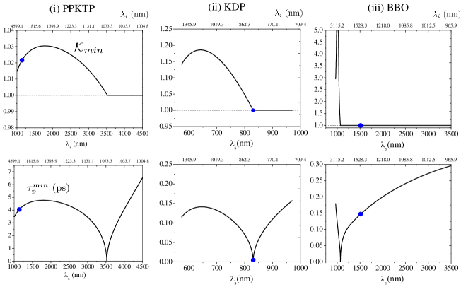
Figure 2: Minimum value of the Schmidt number $K_{min}$ (top panels) and relative pump duration $\tau_{p}^{min}$ (bottom panels) as a function of the signal wavelengths, evaluated with the Gaussian approximation [ Eq.(31) and (30)] for the three crystals chosen as examples. The top horizontal scale shows the conjugate idler wavelength $\lambda_{i}$. The blue dots correspond to the parameters in Table 1

.

Figure 3: Schmidt number ${\cal K}$ evaluated with the Gaussian approximation (28) as a function of the pump pulse duration $\tau_{p}$ for the three examples in Table.1

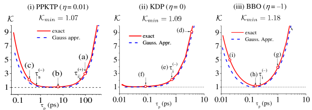
Figure 4: Schmidt number ${\cal K}$ as a function of the pump pulse duration $\tau_{p}$ for the (i) KTP counter-propagating case, (ii) KDP co-propagating and (iii) BBO co-propagating cases (parameters in Table 1). In (i) the state state is nearly separable for pump durations $\tau_{p}$ intermediate between ${\tau_{p,s}^{\text{\tiny{($-$)}}}}=0.67$ps and ${\tau_{p,i}^{\text{\tiny{($+$)}}}}=63$ps. For the co-propagating cases (ii) and (iii), separability is achieved only for subpicosecond pulses with $\tau_{p}\ll{\tau_{p,i}^{\text{\tiny{($-$)}}}}$. The minima of ${\cal K}$, i.e. the amount of achievable separability, are comparable in the three cases. The hollow red dots correspond to the plots shown in Fig.5.

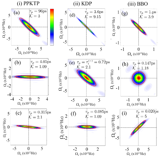
Figure 5: Spectral biphoton correlation $|\psi(\Omega_{s},\Omega_{i})|^{2}$ plotted for decreasing pump pulse duration (from top to bottom) corresponding to the hollow red dots shown in Fig.4. In the short pulse PPKTP case, (c) the idler frequency scale $\Omega_{i}$ is zoomed by factor 10 with respect to the signal frequency scale. The red ellipses corresponds to Eq.(36).

Fig. 2 plots the results of the Gaussian approximation for $K_{min}$ and $\tau_{p}^{min}$ [Eqs. (31) and (30)], as a function of the signal central wavelengths $\lambda_{s}$, for these three examples. The phase-matched wavelengths, $\lambda_{s}$ and $\lambda_{i}$, and the corresponding characteristic times ${\tau_{p,s}^{\text{\tiny{($-$)}}}}$ and ${\tau_{p,i}^{\text{\tiny{($\pm$)}}}}$ are evaluated using the Sellmeier dispersion formula reported in Gurzadian et al. (1991); Kato and Takaoka (2002); Zernike (1964). For the PPKTP crystal, different wavelengths corresponds to different poling periods $\Lambda$, not reported in the figure. For the bulk KDP and BBO crystals the signal and idler central wavelengths are varied by changing the tuning angle $\theta_{p}$ between the pump direction and the crystal axis (not reported in the figure). Notice that in the BBO case $\eta$ is always negative for $\lambda_{s}>1070\,$nm, so that the generated two-photon state is separable when the crystal is tuned on those wavelengths according to approximation (31). Notice also that for $\lambda_{s}=1010\,$nm the group velocities of the signal and idler fields becomes equal ($\eta=1$) and the Schmidt number predicted by Eq.(28) goes to infinity. Under these conditions the SPDC bandwidths and the number entangled modes are in fact very large, through not infinite, as they are only limited by group-velocity dispersion, a feature not taken into account in the simplified model based the linearized phase-matching function (9).

Figures 3 and 4 illustrate the behaviour of the Schmidt number ${\cal K}$ as a function of the the pump pulse duration. The phase-matching conditions for the three crystals are those reported in Table 1 and correspond to the blue dots in Fig.2. Figure 3 reports the results of the Gaussian approximation (28) in linear scale (to allow immediate comparison between the three cases), while Fig. 4 compares the approximate results with the more exact ones obtained through numerical integration of Eqs.(18)-(20). In this latter case dispersion is fully taken into account, the phase-mismatch functions (8) being evaluated using the complete Sellmeier formula. The logarithmic horizontal scale used in this case evidences the different ranges of pump durations $\tau_{p}$ which must be used for achieving separability in the various configurations.

From these plots one can notice that in order to achieve separability the two co-propagating configurations require supbicosecond pulses, whose duration must be close to $\tau_{p}^{min}=147$fs in the BBO case, ${\tau_{\mathrm{p}}}\ll{\tau_{p,i}^{\text{\tiny{($-$)}}}}=720$fs in the KDP case. In contrast, the counter-propagating geometry displays a negligible amount of entanglement over a broad plateau ranging from $\tau_{p}\sim 2$ps up to $\tau_{p}\sim 10$ps.

Figure 4 displays some discrepancy between the approximated results (28) and the exact one especially for short pump pulses, where dispersion plays an important role due to the large bandwidths involved and the phase-matching function mainly determines the twin photon correlation. In particular, the minimum value of ${\cal K}$ is always slightly larger than the value predicted by the Gaussian result (31) and never reaches unity even in the two examples with $\eta\leq 0$. Actually, the amount of purity which can be achieved in the counter-propagating geometry is comparable to that of the two other configurations, which require much more stringent phase matching conditions and ultra-short pulses.
We also notice that the sidelobes of the sinc function (clearly visible e.g. in Fig.5h) are not taken into account by approximation (22) and lead to a slight increase of the amount of entanglement with respect to the prediction of relation (28) in all cases. Branczyk et al. Brańczyk et al. (2011) demonstrated the possibility to eliminate the residual entanglement associated to these sidelobes by modifying the periodic poling of the $\chi^{(2)}$ nonlinearity in order to produce a Gaussian-shaped phase matching function.

Figure 5 shows the biphoton correlation $|\psi(\Omega_{s},\Omega_{i})|^{2}$ in the signal-idler frequency plane. For each crystals (i), (ii) and (iii), the pump pulse duration decreases from top to bottom (the value of $\tau_{p}$ corresponds to the large hollow dots shown in Fig.4). The red ellipses superimposed to the density plots show the curve

$$c_{11}\Omega_{s}^{2}+c_{22}\Omega_{i}^{2}+2c_{12}\Omega_{s}\Omega_{i}=1$$ (36)

where according to the Gaussian formula (24) $|\psi|^{2}$ reduces by a factor $1/e^{2}$. Its principal major axis forms an angle $\theta$ with the $\Omega_{s}$-axis given by

$$\theta=-\frac{1}{2}\arctan\left(\frac{(\tau_{p}/{\tau_{p,i}^{\text{\tiny{($\pm$)}}}})^{2}+2\gamma\eta}{\gamma(1-\eta^{2})}\right)$$ (37)

We have then the following limiting behaviours

$$\theta\to-\frac{\pi}{4}\;\;\text{for}\;\tau_{p}\gg|{\tau_{p,i}^{\text{\tiny{($\pm$)}}}}|$$ (38)

$$\theta\to-\arctan\eta\;\;\text{for}\;\begin{cases}\tau_{p}\ll|{\tau_{p,s}^{\text{\tiny{($-$)}}}}|&\text{if}\;\eta\neq 0\\ \tau_{p}\ll|{\tau_{p,i}^{\text{\tiny{($\pm$)}}}}|&\text{if}\;\eta=0\end{cases}$$ (39)

The first limit, with $\tau_{p}\gg|{\tau_{p,i}^{\text{\tiny{($\pm$)}}}}|$, corresponds to a nearly monochromatic pump pulse with the two-photon state strongly entangled in frequencies. Accordingly, the spectral two-photon amplitude $\psi$ develops along the $\Omega_{i}=-\Omega_{s}$ diagonal, where energy conservation takes place (see panels (a),(d) and (g) in Fig.5).

In the counter-propagating geometry of the PPKTP crystal (i), the state appears separable (the ellipse has its axes aligned with $\Omega_{s}$ and $\Omega_{i}$) for pulses of several picoseconds such that ${\tau_{p,s}^{\text{\tiny{($-$)}}}}\ll{\tau_{\mathrm{p}}}\ll{\tau_{p,s}^{\text{\tiny{($-$)}}}}$, as shown in Fig.5b. Only for very short pump pulses with $\tau_{p}\ll{\tau_{p,s}^{\text{\tiny{($-$)}}}}$, phase-matching determines correlation with $\psi$ aligned along the line $\Omega_{i}=-\eta\Omega_{s}$ (Fig.5c).

In the co-propagating configurations (ii) and (iii), separability is only achieved for pulses in the subpicosecond range satisfying the condition $\tau_{p}\ll|{\tau_{p,i}^{\text{\tiny{($-$)}}}}|$. In the KDP case the two-photon state remains separable for $\tau_{p}\rightarrow 0$ as a consequence of the group-velocity matching of the signal and pump photons ($\eta=0$). For the BBO crystal with symmetrical group velocity matching ($\eta=-1$), the biphoton correlation displays a nearly circular symmetry for $\tau_{p}=\tau_{p}^{min}=147$fs (Fig.5h). In this latter case the frequencies becomes again correlated for ultra-short pulses, the correlations developing along the $\Omega_{s}=\Omega_{i}$ diagonal (Fig.5i).

IV Spectral properties of twin photons

The Gaussian approximation also allows an immediate comparison of the spectral properties of the twin photons generated in the various configurations, by calculating their first order coherence functions. By inserting the Gaussian formula for the biphoton amplitude inside Eqs. (16,17), we get

$$G_{s}^{(1)}(\Omega_{s},\Omega_{s}^{\prime}) \approx\frac{g^{2}\tau_{p}^{2}}{\sqrt{8\pi c_{22}}}e^{-i{\tau_{p,s}^{\text{\tiny{($-$)}}}}(\Omega_{s}-\Omega_{s}^{\prime})}$$

$$\times e^{-\frac{2c_{11}c_{22}-c_{12}^{2}}{2c_{22}}(\Omega_{s}^{2}+\Omega_{s}^{\prime 2})+\frac{c_{12}^{2}}{c_{22}}\Omega_{s}\Omega_{s}^{\prime}}$$ (40)

$$G_{i}^{(1)}(\Omega_{i},\Omega_{i}^{\prime}) \approx\frac{g^{2}\tau_{p}^{2}}{\sqrt{8\pi c_{11}}}e^{-i{\tau_{p,i}^{\text{\tiny{($\pm$)}}}}(\Omega_{i}-\Omega_{i}^{\prime})}$$

$$\times e^{-\frac{2c_{11}c_{22}-c_{12}^{2}}{2c_{11}}(\Omega_{i}^{2}+\Omega_{i}^{\prime 2})+\frac{c_{12}^{2}}{c_{11}}\Omega_{i}\Omega_{i}^{\prime}}$$ (41)

Using these formulas, we can estimate the bandwidths $\sigma_{j}$ of the signal and idler spectra

$${\cal S}_{j}(\Omega_{j}):=G_{j}^{(1)}(\Omega_{j},\Omega_{j})\propto e^{-\frac{\Omega_{j}^{2}}{2\sigma_{j}^{2}}}\;\;(j=i,s).$$ (42)

Expliciting the $c_{ij}$ coefficients given in Eqs.(25)-(27), we find

$$\sigma_{s} = \frac{1}{\sqrt{2}(1-\eta)}\left(\frac{1}{2\gamma{\tau_{p,i}^{\text{\tiny{($\pm$)}}}}^{2}}+\frac{1}{\tau_{p}^{2}}\right)^{1/2}$$ (43)

$$\sigma_{i} = \frac{1}{\sqrt{2}(1-\eta)}\left(\frac{1}{2\gamma{\tau_{p,i}^{\text{\tiny{($\pm$)}}}}^{2}}+\frac{\eta^{2}}{\tau_{p}^{2}}\right)^{1/2}$$ (44)

Considering the particular cases in which the state becomes separable or nearly separable (corresponding to the examples shown in the panels (b), (f) and (h) of Fig.5), we have

$$\sigma_{s} \approx \begin{cases}\frac{1}{\sqrt{2}\tau_{p}^{min}}&\text{case {\bf(i)}}:|\eta|\ll 1,\;\tau_{p}=\tau_{p}^{min}\\ \frac{1}{\sqrt{2}\tau_{p}}&\text{case {\bf(ii)}}:\eta=0,\;\tau_{p}\ll|{\tau_{p,i}^{\text{\tiny{($-$)}}}}|\\ \frac{1}{2\tau_{p}^{min}}&\text{case {\bf(iii)}}:\eta=-1,\;\tau_{p}=\tau_{p}^{min}\end{cases}$$ (45)

$$\sigma_{i} \approx \begin{cases}\frac{1}{2\sqrt{\gamma}|{\tau_{p,i}^{\text{\tiny{($+$)}}}}|}\;\;&\text{case {\bf(i)}}:|\eta|\ll 1,\;\tau_{p}=\tau_{p}^{min}\\ \frac{1}{2\sqrt{\gamma}|{\tau_{p,i}^{\text{\tiny{($-$)}}}}|}&\text{case {\bf(ii)}}:\eta=0,\tau_{p}\ll|{\tau_{p,i}^{\text{\tiny{($-$)}}}}|\\ \frac{1}{2\tau_{p}^{min}}\;\;&\text{case {\bf(iii)}}:\eta=-1,\;\tau_{p}=\tau_{p}^{min}\end{cases}$$ (46)

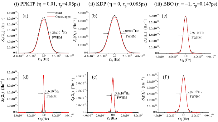
Figure 6: Spectra of the signal (top) and of the idler (bottom) for the three examples considered, in conditions of nearly separability of the state corresponding to panels (b), (f), and (h) of Fig.5. Black lines: numerical results from Eqs.(16),(17). Red lines: Gaussian approximation (40),(41). The indicated bandwidths (FWHM) are calculated from the ”exact ” numerical results and match the approximated ones in Eqs.(45)-(46) within an error of less than 10%.

Fig.6 plots the spectra of the signal and idler photons, in the optimal conditions for separability, calculated both with this Gaussian approximation and with the more exact numerical integration of Eqs. (16)-(17). From this figure and from the approximated results in Eqs. (45) (46), we observe that in conditions of separability :

1. In all the cases, the bandwidth of the signal photon reproduces basically that of the pump laser (a part some inessential $\sqrt{2}$ factors). Clearly, in the counter-propagating configuration it is much narrower (less than ThZ) than in the co-propagating case, because separability is achieved in the former case for longer pump pulses.

2. The bandwidth of the idler photon is rather determined by the phase-matching characteristic time ${\tau_{p,i}^{\text{\tiny{($\pm$)}}}}$ (notice that in case ( iii), of symmetric group-velocity matching, the two bandwidths coincides since $\tau_{p}^{min}=\sqrt{2\gamma}|{\tau_{p,i}^{\text{\tiny{($-$)}}}}|$). As expected, the bandwidth of the backward propagating idler is more than two order of magnitude narrower than those of the co-propagating idler photons, because the GVS characteristic time ${\tau_{p,i}^{\text{\tiny{($+$)}}}}$ is two orders of magnitude longer than than the GVM characteristic times involved in the co-propagating cases.

V Conclusions

In this work we compared different phase-matching configurations suitable for generating pure heralded single photons from spontaneous parametric down-conversion. We provided a detailed analysis of the conditions under which separable twin twin photons can be generated through the quantitative evaluation of the Schmidt number as a function of the pump pulse duration. Because of the natural separation of the GVM and the GVS time scales ${\tau_{p,s}^{\text{\tiny{($-$)}}}}$ and ${\tau_{p,i}^{\text{\tiny{($+$)}}}}$, the counter-propagating geometry offers the advantage of generating separable twin photons without the need to fine tune their relative group-velocities as in standard co-propagating configurations. Because of this unique feature, counter-propagating twin photons in a pure state can in principle be heralded at any frequency by choosing the required poling period. Moreover, the twin photons are naturally narrow band, especially the one propagating opposite to the pump direction, and separability is achieved for a broad range of pump pulse durations within ${\tau_{p,s}^{\text{\tiny{($-$)}}}}$ and ${\tau_{p,i}^{\text{\tiny{($+$)}}}}$.

In contrast, twin photons emitted in the common co-propagating geometry are naturally broadband and can be generated in a separable state only for very short pulses, under particular phase-matching conditions and at particular wavelengths depending on the material. The counter-propagating configuration offers thus much more flexibility, once the technical challenges for the fabrication of crystals with sub-micrometric poling periods are overcomed.

References

- Gatti et al. (2015) A. Gatti, T. Corti, and E. Brambilla, Phys. Rev. A 92, 053809 (2015).
- Grice et al. (2001) W. P. Grice, A. B. U’Ren, and I. A. Walmsley, Phys. Rev. A 64, 063815 (2001).
- U’Ren et al. (2006) A. B. U’Ren, C. Silberhorn, K. Banaszek, I. A. Walmsley, R. Erdmann, W. P. Grice, and M. G. Raymer, Laser Physics 15, 146–161 (2006).
- Mosley et al. (2008a) P. J. Mosley, J. S. Lundeen, B. J. Smith, P. Wasylczyk, A. B. U’Ren, C. Silberhorn, and I. A. Walmsley, Phys. Rev. Lett. 100, 133601 (2008a).
- Migdall et al. (2002) A. L. Migdall, D. Branning, and S. Castelletto, Phys. Rev. A 66, 053805 (2002).
- Levine et al. (2010) Z. H. Levine, J. Fan, J. Chen, A. Ling, and A. Migdall, Opt. Expr. 18, 3708 (2010).
- Bennink (2010) R. S. Bennink, Phys. Rev. A 81, 053805 (2010).
- Brańczyk et al. (2011) A. M. Brańczyk, A. Fedrizzi, T. M. Stace, T. C. Ralph, and A. G. White, Opt. Express 19, 55 (2011).
- Zhang et al. (2012) L. Zhang, C. Soeller, O. Cohen, B. J. Smith, and I. A. Walmsley, J. of Mod. Optics 59, 1525 (2012).
- Migdall et al. (2013) A. Migdall, S. Polyakov, J. Fan, and J. Bienfang, eds., Single-Photon Generation and Detection: Physics and Applications, Experimental Methods in the Physical Sciences, Vol. 45 (Academic Press, 2013).
- Harris (1966) S. E. Harris, Appl. Phys. Lett. 9, 114 (1966).
- Canalias and Pasiskevicius (2007) C. Canalias and V. Pasiskevicius, Nat. Photon. 1, 459 (2007).
- Canalias et al. (2003) C. Canalias, V. Pasiskevicius, R. Clemens, and F. Laurell, Appl. Phys. Lett. 82, 4233 (2003).
- Pasiskevicius et al. (2012) V. Pasiskevicius, G. Strömqvist, F. Laurell, and C. Canalias, Opt. Materials 34, 513 (2012).
- Strömqvist et al. (2012) G. Strömqvist, V. Pasiskevicius, C. Canalias, P. Aschieri, A. Picozzi, and C. Montes, J. Opt. Soc. Am. B 29, 1194 (2012).
- Suhara and Ohno (2010) T. Suhara and M. Ohno, IEEE Journal of Quantum Electronics 46, 1739 (2010).
- Corti et al. (2016) T. Corti, E. Brambilla, and A. Gatti, Phys. Rev. A 93, 023837 (2016).
- Christ et al. (2009) A. Christ, A. Eckstein, P. J. Mosley, and C. Silberhorn, Opt. Expr. 17, 3441 (2009).
- Evans et al. (2010) P. G. Evans, R. S. Bennink, W. P. Grice, T. S. Humble, and J. Schaake, Phys. Rev. Lett. 105, 253601 (2010).
- Ekert and Knight (1995) A. Ekert and P. L. Knight, American Journal of Physics 63, 415 (1995).
- Parker et al. (2000) S. Parker, S. Bose, and M. B. Plenio, Phys. Rev. A 61, 032305 (2000).
- van Exter et al. (2006) M. P. van Exter, A. Aiello, S. S. R. Oemrawsingh, G. Nienhuis, and J. P. Woerdman, Phys. Rev. A 74, 012309 (2006).
- Gatti et al. (2012) A. Gatti, T. Corti, E. Brambilla, and D. B. Horoshko, Phys. Rev. A 86, 053803 (2012).
- Mikhailova et al. (2008) Y. M. Mikhailova, P. A. Volkov, and M. V. Fedorov, Phys. Rev. A 78, 062327 (2008).
- Gurzadian et al. (1991) G. G. Gurzadian, V. G. Dmitriev, and D. N. Nikogosian, Handbook of nonlinear optical crystals (Springer-Verlag Berlin, New York, 1991).
- Kato and Takaoka (2002) K. Kato and E. Takaoka, Appl. Opt. 41, 5040 (2002).
- Zernike (1964) F. Zernike, J. Opt. Soc. Am. 54, 1215 (1964).
- Law and Eberly (2004) C. K. Law and J. H. Eberly, Phys. Rev. Lett. 92, 127903 (2004).
- Mosley et al. (2008b) P. J. Mosley, J. S. Lundeen, B. J. Smith, and I. A. Walmsley, New Journal of Physics 10, 093011 (2008b).