Dynamics of two disks settling in a two-dimensional narrow channel: From periodic motion to vertical chain in Oldroyd-B fluid

Abstract

In this article we present a numerical study of the dynamics of two disks settling in a narrow vertical channel filled with Oldroyd-B fluid. Two kinds of particle dynamics are obtained: (i) periodic interaction between two disks and (ii) the chain formation of two disks. For the periodic interaction of two disks, two different motions are obtained: (a) two disks stay far apart and interact periodically and (b) two disks interact closely and then far apart in a periodic way, like the drafting, kissing and tumbling of two disks sedimenting in Newtonian fluid, due to the lack of strong enough elastic force. For the formation of two disk chain occurred at higher values of the elasticity number, it is either a tilted chain or a vertical chain. The tilted chain can be obtained for either that the elasticity number is less than the critical value for having the vertical chain or that the Mach number is greater than the critical value for a long body to fall broadside-on. Hence the values of the elasticity number and the Mach number determine whether the the chain can be formed and the orientation of the chain.

Keywords: Sedimentation, Chaining, periodic motion, particles, Oldroyd-B fluid

1 Introduction

The motion of particles in non-Newtonian fluids is not only of fundamental theoretical interest, but is also of importance in many applications to industrial processes involving particle-laden materials (see, e.g., [1] and [2]). For example, during the hydraulic fracturing operation used in oil and gas wells, suspensions of solid particles in polymeric solutions are pumped into hydraulically-induced fractures. The particles must prop these channels open to enhance the rate of oil recovery [3]. During the shut-in stage, proppant settling is pronounced when the fluid pressure decreases due to the end of hydraulic fracturing process. The study of particle chain during settling in vertical channel can help us to understand the mechanism of proppant agglomeration in narrow fracture zones. There have been works on the simulation of the sedimentation of particles in Oldroyd-B fluids in, e.g., [4], [5], [6], [7], [8], [9] and references given in a review article [10]. Feng et al. study the two-dimensional sedimentation of circular particles in an Oldroyd-B fluid. They obtained chains of two particles aligned with the direction of sedimentation, which is precisely the microstructure observed in actual experiments [11]. In [6], an arbitrary Lagrangian-Eulerian (ALE) moving mesh technique (see [5]) was used to investigate the cross-stream migration and orientations of elliptic particles in Oldroyd-B fluids (with and without shear thinning). Huang et al. found that the orientation of elliptic particles depends on two critical numbers, the elasticity and Mach numbers. In [7], a fictitious domain/distributed Lagrange multiplier (FD/DLM) method for particulate flow of Oldroyd-B fluids was developed and chains of two particles aligned with the direction of sedimentation were obtained and for the case of multiple circular particles, many chains of two particles were found next to the channel walls. Shao and Yu [8] used an improved FD/DLM method to obtain that the stable configuration is the one where the particles are aligned parallel to the flow direction when the Mach number the elasticity number are in the range discussed in [6].

Although numerical methods for simulating particulate flows in Newtonian fluids have been very successful, numerically simulating particulate flows in viscoelastic fluids is much more complicated and challenging. One of the difficulties (e.g., see [12], [13]) for simulating viscoelastic flows is the breakdown of the numerical methods. It has been widely believed that the lack of positive definiteness preserving property of the conformation tensor at the discrete level during the entire time integration is one of the reasons for the breakdown. To preserve the positive definiteness property of the conformation tensor, several methodologies have been proposed recently, as in [14], [15], [16] and [17]. Lozinski and Owens [17] factored the conformation tensor to get ${\boldsymbol{\sigma}}=AA^{t}$ and then they wrote down the equations for $A$ approximately at the discrete level. Hence, the positive definiteness of the conformation tensor is forced with such an approach. The methodologies developed in [17] have been applied in [9] together with the FD/DLM method through operator splitting techniques for simulating particulate flows in Oldroyd-B fluid. In this article, the computational results of two disks settling in Oldroyd-B fluids are obtained by the numerical method developed in [9].

It is known that particle settling in a viscoelastic fluid can be quite different from that which is observed in Newtonian fluids. A well-known one for two disk interaction can be described as drafting, kissing and tumbling in Newtonian fluids [18] and as drafting, kissing and chaining in viscoelastic fluids. In this article, we have studied the dynamics of two disks settling in a narrow vertical channel filled with an Oldroyd-B fluid, which covers not only the vertical chain of two disks but also the tilted chain of two disks and the periodic motion of two disks interacting with each other. We have obtained that the formation and orientation of particle chain depends on the value of the elasticity number and that of the Mach number as discussed in [6] for elliptic particles settling Oldroyd-B fluids since a chain of two disks is a long body even they are loosely coupled. But for the lower values of the elasticity number, we have obtained that two disks interact with each other periodically in two different ways. One of them is that two disks interact far apart in a periodic way, which is close to the one discussed in [19] for two disks settling in Newtonian fluid in the lower Reynolds number regime (not the drafting, kissing and tumbling phenomenon). The other one is close to the drafting, kissing and chaining in viscoelastic fluid; but the last part, chaining, can not be completed due to the lack of strong enough elastic force to hold them together. The article is organized as follows. In Section 2, we present a FD/DLM formulation for particulate flows in Oldroyd-B fluid and briefly discuss the associated the operator splitting technique, the space and time discretization of the FD/DLM formulation. In Section 3, numerical results of the cases of sedimentation of two disks and their chaining are discussed.

2 Mathematical Formulations and numerical methods

2.1 Governing equations and its FD/DLM Formulation

Following the work developed in [9], we will first address in the following the models and computational methodologies. Let $\Omega$ be a bounded two-dimensional (2D) domain and let $\Gamma$ be the boundary of $\Omega$. We suppose that $\Omega$ is filled with a viscoelastic fluid of an Oldroyd-B fluid of density $\rho_{f}$ and that it contains $N$ moving rigid particles of density $\rho_{s}$ (see Figure 1). Let $B(t)=\displaystyle\cup_{i=1}^{N}B_{i}(t)$ where $B_{i}(t)$ is the $i$th rigid particle in the fluid for $i=1,\dots,N$. We denote by $\partial B_{i}(t)$ the boundary of $B_{i}(t)$ for $i=1,\dots,N$. For some $T>0,$ the governing equations for the fluid-particle system are

$$\hskip-20.0pt\rho_{f}(\dfrac{\partial{\bf u}}{\partial t}+({\bf u}\cdot{\boldsymbol{\nabla}}){\bf u})=\rho_{f}{\bf g}-{\boldsymbol{\nabla}}p+2\mu{\boldsymbol{\nabla}}\cdot{\bf D}({\bf u})+{\boldsymbol{\nabla}}\cdot{\boldsymbol{\sigma}}^{p}\ \ in\ \Omega\backslash\overline{B(t)},\,t\in(0,T),$$ (1)

$$\hskip-20.0pt\ \nabla\cdot\textbf{u}=0\ \ in\ \Omega\backslash\overline{B(t)},\,t\in(0,T),$$ (2)

$$\hskip-20.0pt\ {\bf u}({\bf x},0)={\bf u}_{0}({\bf x}),\ \ \forall{\bf x}\in\Omega\backslash\overline{B(0)},\ with\,\nabla\cdot{\bf u}_{0}=0,$$ (3)

$$\hskip-20.0pt\ {\bf u}={\bf g}_{0}\ \ on\ \Gamma\times(0,T),with\int_{\Gamma}{\bf g}_{0}\cdot{\bf n}\,d\Gamma=0,$$ (4)

$$\hskip-20.0pt\ {\bf u}={{\bf V}}_{p,i}+\omega_{i}\times\stackrel{{\scriptstyle\longrightarrow}}{{{\bf G}_{i}{\bf x}}},\ \forall{\bf x}\in\partial B_{i}(t),\,i=1,\cdots,N,$$ (5)

$$\hskip-20.0pt\dfrac{\partial{\bf C}}{\partial t}+({\bf u}\cdot{\boldsymbol{\nabla}})\ {\bf C}-({\boldsymbol{\nabla}}{\bf u})\ {\bf C}-{\bf C}\ ({\boldsymbol{\nabla}}{\bf u})^{t}=-\dfrac{1}{\lambda_{1}}({\bf C}-{\bf I})\,\,\,in\ \Omega\backslash\overline{B(t)},\,t\in(0,T),$$ (6)

$$\hskip-20.0pt\ {\bf C}({\bf x},0)={\bf C}_{0}({\bf x}),\,{\bf x}\in\Omega\backslash\overline{B(0)},$$ (7)

$$\hskip-20.0pt\ {\bf C}={\bf C}_{L},\ \ on\ \Gamma^{-},$$ (8)

where ${\bf u}$ is the flow velocity, $p$ is the pressure, ${\bf g}$ is the gravity, $\mu=\eta_{1}\lambda_{2}/\lambda_{1}$ is the solvent viscosity of the fluid, $\eta=\eta_{1}-\mu$ is the elastic viscosity of the fluid, $\eta_{1}$ is the fluid viscosity, $\lambda_{1}$ is the relaxation time of the fluid, $\lambda_{2}$ is the retardation time of the fluid, ${\bf n}$ is the outer normal unit vector at $\Gamma,$ $\Gamma^{-}$ is the upstream portion of $\Gamma$. The polymeric stress tensor ${\boldsymbol{\sigma}}^{p}$ in (1) is given by ${\boldsymbol{\sigma}}^{p}=\dfrac{\eta}{\lambda_{1}}({\bf C}-{\bf I})$, where the conformation tensor ${\bf C}$ is symmetric and positive definite (see [20]) and ${\bf I}$ is the identity matrix.

Figure 1: An example of a two-dimensional flow region with four circular particles.

In (5), the no-slip condition holds on the boundary of the $i$th particle, ${\bf V}_{p,i}$ is the translation velocity, $\omega_{i}$ is the angular velocity and ${\bf G}_{i}$ is the center of mass and $\omega_{i}\times\stackrel{{\scriptstyle\longrightarrow}}{{{\bf G}_{i}{\bf x}}}=(-\omega_{i}(x_{2}-G_{i,2}),\omega_{i}(x_{1}-G_{i,1}))$ (for 2D cases considered in this article). The motion of the particles is modeled by Newton’s laws:

$$M_{p,i}\ \dfrac{d{\bf V}_{p,i}}{dt}=M_{p,i}{\bf g}+{\bf F}_{i}+{\bf F}_{i}^{r},$$ (9)

$$I_{p,i}\dfrac{d\omega_{i}}{dt}=F^{t}_{i},$$ (10)

$$\dfrac{d{\bf G}_{i}}{dt}={\bf V}_{p,i},$$ (11)

$${\bf G}_{i}(0)={\bf G}^{0}_{i},{\bf V}_{p,i}(0)={\bf V}^{0}_{p,i},\omega_{i}(0)={\omega}^{0}_{i},$$ (12)

for $i=1,\dots,N$, where in (9)-(12), $M_{p,i}$ and $I_{p,i}$ are the the mass and the inertia of the $i$th particle, respectively, ${\bf F}^{r}_{i}$ is a short range repulsion force imposed on the $i$th particle by other particles and the wall to prevent particle/particle and particle/wall penetration (see [21] for details), and ${\bf F}_{i}$ and ${F}^{t}_{i}$ denote the hydrodynamic force and the associated torque imposed on the $i$th particle by the fluid, respectively.

To avoid the frequent remeshing and the difficulty of the mesh generation for a time-varying domain in which the rigid particles can be very close to each other, especially for three dimensional particulate flow, we have extended the governing equations to the entire domain $\Omega$ (a fictitious domain). For a fictitious-domain-based variational formulation of the governing equations of the particulate flow, we consider only one rigid particle $B(t)$ (a disk in 2D) in the fluid domain without losing generality. Let us define first the following functional spaces

$${\bf V}_{{\bf g}_{0}(t)}=\{\ {\bf v}\ |\ {\bf v}\ \in({H^{1}(\Omega)})^{2},{\bf v}={\bf g}_{0}(t)\ on\ \Gamma\},$$

$$L_{0}^{2}(\Omega)=\{\ q\ |\ q\ \in{L^{2}(\Omega)},\int_{\Omega}q\,d{\bf x}=0\},$$

$${\bf V}_{{\bf C}_{L}(t)}=\{\ {\bf C}\ |\ {\bf C}\ \in({H^{1}(\Omega)})^{2\times 2},{\bf C}={\bf C}_{L}(t)\ on\ \Gamma^{-}\},$$

$${\bf V}_{{\bf C}_{0}}=\{\ {\bf C}\ |\ {\bf C}\ \in({H^{1}(\Omega)})^{2\times 2},{\bf C}=0\ on\ \Gamma^{-}\},$$

$$\Lambda(t)={H^{1}(B(t))}^{2}.$$

Following the methodologies developed in [7, 21], a fictitious domain formulation of the governing equations (1)-(12) reads as follows:

For a.e. $t>0,$ find ${\bf u}(t)\in{\bf V}_{{\bf g}_{0}(t)}$, $p(t)\in L_{0}^{2}(\Omega)$, ${\bf C}(t)\in{\bf V}_{{\bf C}_{L}(t)}$, ${\bf V}(t)\in{\text{I\!R}}^{2}$, ${\bf G}(t)\in{\text{I\!R}}^{2}$, $\omega(t)\in{\text{I\!R}}$, ${\boldsymbol{\lambda}}(t)\in\Lambda(t)$ such that

$$\begin{cases}\displaystyle\rho_{f}\int_{\Omega}\left[\dfrac{\partial{\bf u}}{\partial t}+({\bf u}\cdot{\boldsymbol{\nabla}}){\bf u}\right]\cdot{\bf v}\,d{\bf x}+2\mu\int_{\Omega}{\bf D}({\bf u}):{\bf D}({\bf v})\,\,d{\bf x}-\int_{\Omega}p{\boldsymbol{\nabla}}\cdot{\bf v}\,d{\bf x}\\ \displaystyle-\int_{\Omega}{\bf v}\cdot({\boldsymbol{\nabla}}\cdot{\boldsymbol{\sigma}}^{p})\,\,d{\bf x}+(1-\rho_{f}/\rho_{s})\{M_{p}\dfrac{d{\bf V}}{dt}\cdot{\bf Y}+I_{p}\dfrac{d\omega}{dt}\cdot\theta\}\\ \displaystyle-<{\boldsymbol{\lambda}},{\bf v}-{\bf Y}-\theta\times{\stackrel{{\scriptstyle\longrightarrow}}{{{\bf G}{\bf x}}}}>_{B(t)}-{\bf F}^{r}\cdot{\bf Y}\\ \displaystyle=\rho_{f}\int_{\Omega}\mathbf{g}\cdot\mathbf{v}d\mathbf{x}+(1-\rho_{f}/\rho_{s})M_{p}{\bf g}\cdot{\bf Y},\\ \displaystyle\forall\{{\bf v},{\bf Y},\theta\}\in(H_{0}^{1}(\Omega))^{2}\times{\text{I\!R}}^{2}\times{\text{I\!R}},\end{cases}$$ (13)

$$\int_{\Omega}q{\boldsymbol{\nabla}}\cdot{\bf u}(t)\,d{\bf x}=0,\forall q\in L^{2}(\Omega),$$ (14)

$$<{\boldsymbol{\mu}},{\bf u}({\bf x},t)-{\bf V}(t)-\omega(t)\times{\stackrel{{\scriptstyle\longrightarrow}}{{{\bf G}(t){\bf x}}}}>_{B(t)}=0,\ \ \forall{\boldsymbol{\mu}}\in{\boldsymbol{\Lambda}}(t),$$ (15)

$$\int_{\Omega}\left(\dfrac{\partial{\bf C}}{\partial t}+({\bf u}\cdot{\boldsymbol{\nabla}}){\bf C}-({\boldsymbol{\nabla}}{\bf u}){\bf C}-{\bf C}({\boldsymbol{\nabla}}{\bf u})^{t}\right):{\bf s}\,d{\bf x}$$ (16)

$$=-\int_{\Omega}\dfrac{f({\bf C})}{\lambda_{1}}({\bf C}-{\bf I}):{\bf s}\,d{\bf x},\forall{\bf s}\in{\bf V}_{{\bf C}_{0}},\ with\ \ {\bf C}={\bf I}\ \ in\ \ B(t),$$

$$\dfrac{d{\bf G}}{dt}={\bf V},$$ (17)

$${\bf C}({\bf x},0)={\bf C}_{0}({\bf x}),\forall{\bf x}\in\Omega,\ with\ \ {\bf C}_{0}={\bf I}\ \ in\ \ B(0),$$ (18)

$${\bf G}(0)={\bf G}_{0},\ {\bf V}(0)={\bf V}_{0},\ \omega(0)=\omega_{0},\ B(0)=B_{0},$$ (19)

$${\bf u}({\bf x},0)=\begin{cases}{\bf u}_{0}({\bf x}),\forall{\bf x}\in\Omega\setminus{\overline{B_{0}}},\\ {\bf V}_{0}+\omega_{0}\times{\stackrel{{\scriptstyle\longrightarrow}}{{{\bf G}_{0}{\bf x}}}},\ \forall{\bf x}\in{\overline{B_{0}}}.\end{cases}$$ (20)

In (13) the Lagrange multiplier ${\boldsymbol{\lambda}}$ defined over $B$ can be viewed as an extra body force maintaining the rigid body motion inside $B$. The conformation tensor ${\bf C}$ inside the rigid particle is extended as the identity tensor ${\bf I}$ as in (16) since the polymeric stress tensor is zero inside the rigid particle. In equation (13), since ${\bf u}$ is divergence free and satisfies the Dirichlet boundary conditions on $\Gamma,$ we have $2\int_{\Omega}{\bf D}({\bf u}):{\bf D}({\bf v})\,d{\bf x}=\int_{\Omega}{\boldsymbol{\nabla}}{\bf u}:{\boldsymbol{\nabla}}{\bf v}\,d{\bf x},\,\forall{\bf v}\in(H_{0}^{1}(\Omega))^{2}$. This is a substantial simplification from the computational point of view, which is another advantage of the fictitious domain approach. With this simplification, we can use fast solvers for the elliptic problems in order to speed up computations. Also the gravity term ${\bf g}$ in (13) can be absorbed in the pressure term.

The details of numerical methodologies for simulating the motion of disks sedimenting in Oldroyd-B fluid in a vertical two-dimensional channel are given in [9]. Applying Lie’s scheme to (13)-(20), we have used a seven stage operator-splitting scheme to obtain numerical results, namely: In Stage 1, we use a Neumann preconditioned Uzawa/conjugate gradient algorithm to force (in a $L^{2}$ sense) the incompressibility condition of ${\bf u}$ discussed in [9] and [22]. In Stage 2, we combine two advection steps: one for ${\bf u}$ and one for ${\bf C}$, which are solved by a wave-like equation method (see [22] and [23]) which is an explicit method and does not introduce numerical dissipation. In this stage, we have transformed the advection step for ${\bf C}$ into the one for $A$ like Lozinski and Owens’ work in [17] where ${\bf C}$ is factorized as $AA^{t}$. In Stage 3, we combine a diffusion step for ${\bf u}$ with a step taking into account the remaining operator in the transformed evolution equation verified by $A$. In Stage 4, we update the position of ${\bf G}$. In Stage 5, we force the rigid body motion of the particle and update ${\bf V}$ and $\omega$ by a conjugate gradient method given in e.g., [9] and [22], and then impose the condition ${\bf C}={\bf I}$ inside the particle. In Stage 6, we correct the position of ${\bf G}$ via the updated ${\bf V}$ and $\omega$. Finally, Stage 7 is a diffusion step for the velocity, driven by the updated polymeric stress tensor.

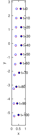
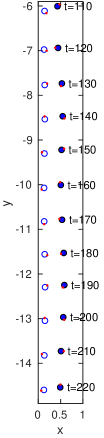
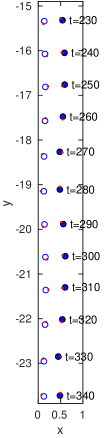
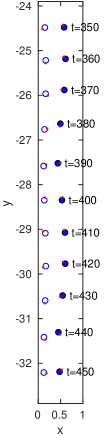
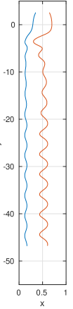
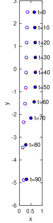
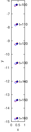
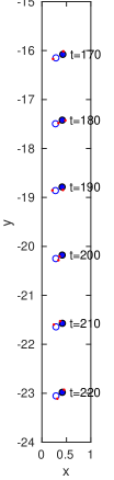
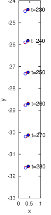
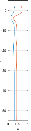
Figure 2: Positions of two disks (left four) and trajectories of two disks (right) for $\rho_{s}=1.0025$ and E=0.16 (the other associate numbers are Re=0.3858, M=0.1453 and De=0.0617).

Figure 3: Positions of two disks (left four) and trajectories of two disks (right) for$\rho_{s}=1.0025$ and E=0.256 (the other associate numbers are Re=0.7222, M=0.3654 and De=0.1848).

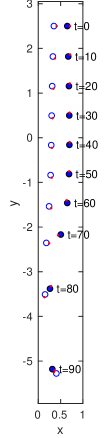
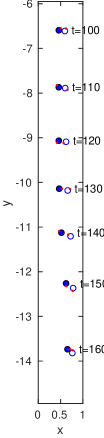
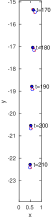
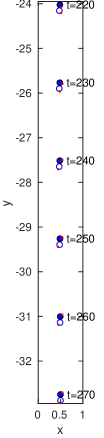
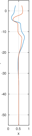
Figure 4: Positions of two disks (left four) and trajectories of two disks (right) for$\rho_{s}=1.0025$ and E=0.32 (the other associate numbers are Re=0.8731, M=0.4939 and De=0.2794).

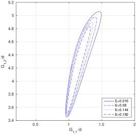
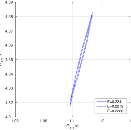
Figure 5: Trajectories of disks in phase space of the normalized distances between the disk mass center and the left wall for $\rho_{s}=1.0025$. The periods are 58.55, 56.80, 55.485 and 54.205 for E=0.016, 0.080, 0.144 and 0.192, respectively (left) and the periods are 52.067, 49 and 47.9 for E=0.224, 0.2272 and 0.2288, respectively (right).

3 Numerical Results and discussion

In the following discussion, the particle Reynolds number is Re$=\dfrac{\rho_{f}Ud}{\eta_{1}}$, the Debra number is De$=\dfrac{\lambda_{1}U}{d}$, the Mack number is M=$\sqrt{\rm DeRe}$, and the elasticity number is E=De/Re=$\dfrac{\lambda_{1}\eta_{1}}{d^{2}\rho_{f}}$ where $U$ is the averaged terminal speed of disks and $d$ is the disk diameter. As discussed in [6] and [24], when the elasticity number E is larger than the critical value ($O(1)$), a long body settling in Oldroyd-B fluids turns its broadside parallel to the flow direction. But for the elasticity number E less than the critical value, it falls steadily in a configuration in which the axis of the long body is at a fixed angle of tilt with the horizontal. Also for larger Mach numbers, the long body flips into broadside on falling again. For the dynamics of two disks settling in Oldroyd-B fluid, they can be viewed as a long body if they form a chain. We like to study the equilibrium orientation of this “long body” of two disk chain by varying the elasticity number. But two disks can stay separated for the smaller value of E, it is interesting to find out how two disks interact and whether such interaction is close to the dynamics of two settling disks in Newtonian fluid such as drafting, kissing and tumbling phenomenon [18] or some kinds of periodic motion discussed in [19]. The computational results of two disk motion in this section are obtained by the numerical method developed in [9].

For all numerical results, we have considered the settling of two disks in a vertical channel of infinite length filled with an Oldroyd-B fluid as in [9], the computational domain is $\Omega=(0,1)\times(0,6)$ initially and then it moves vertically with the mass center of the disk (see, e.g., [25] and [26] and references therein for adjusting the computational domain according to the position of the particle). The two disk diameters are $d=$0.125 and the initial position of the disk centers are at (0.35, 2.5) and (0.65, 2.5), respectively. The disk density $\rho_{s}$ is 1.0025 for first several cases considered in this section and the fluid density $\rho_{f}$ is 1. The fluid viscosity $\eta_{1}$ is 0.025. The relaxation time $\lambda_{1}$ varies between 0.01 and 1.0 and the retardation time $\lambda_{2}$ is $\lambda_{1}/4$. Then the associated elasticity number is E=$1.6\lambda_{1}$. In Figs. 3, 3 and 4, three typical motions of two disks settling in Oldroyd-B fluid are presented. For E=0.16 ($\lambda_{1}=0.1$), the dynamics of two disk interaction is characterized by its periodical motion (of period 55.25 time units) as in Fig. 3, which is similar to the one of the motions of two settling disks in a Newtonian fluid obtained in [19]. For a slightly higher value, E=0.256 ($\lambda_{1}=0.16$), two disks form a chain with a stable tilt angle of 29.39 degrees (see Fig. 3), which is similar to the behavior of a long body when the elasticity number is less than the critical value for turning its broadside parallel to the flow direction. For E=0.32 ($\lambda_{1}=0.2$), we have obtained that two disks form a stable vertical chain as shown in Fig. 4, which indicates the the critical value of the elasticity number for having a vertical chain is somewhere between 0.256 and 0.32.

For more details about the dynamics of two disks, we have obtained the following results by varying the relaxation time $\lambda_{1}$ (resp., the elasticity number) from 0.01 to 1 (resp., from 0.016 to 1.6). For E between 0.016 ($\lambda_{1}$=0.01) and 0.24 ($\lambda_{1}$=0.15), two disks stay separated and their interaction is periodical. For example, in the phase space shown in Fig. 5, constructed by the normalized distances between the disk mass center (${\bf G}_{i}=\{G_{1,i},G_{2,i}\}^{t}$, $i=$1, 2) and the side wall, i.e., $G_{1,1}/d$ and $G_{1,2}/d$, the attractor is a limit cycle for each value of the elasticity number. At E=0.208 ($\lambda_{1}$=0.13), the limit cycle shrinks to about a point. Then another kind of limit cycle occurs for $0.208<{\rm E}\leq 0.2288$ (see Fig. 5). But for $0.2304\leq{\rm E}\leq 0.24$, two disks settle without noticeable periodic motion and remain separated at a constant distance. The gap between two disk decreases when increasing the value of E from 0.2304 to 0.24. For E=0.256 ($\lambda_{1}$ = 0.16) and 0.288 ($\lambda_{1}$ =0.18), two disks form a chain with a stable tilt angle of 29.69 and 82.33 degrees, respectively (see Fig. 3 for E=0.256). Finally, for E between 0.304 ($\lambda_{1}$=0.19 ) and 1.6 ($\lambda_{1}$=1), a vertical chain of two disks is formed. Thus the critical value of the elasticity number for having a vertical chain is somewhere in the interval [0.288, 0.304].

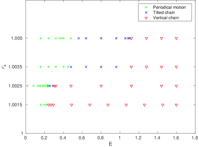
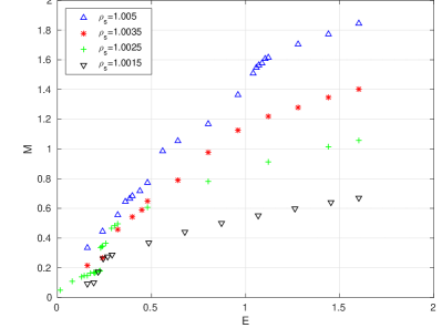
Figure 6: The phase diagram (left) and the associated values of the Mach number (right) of two disk interaction in a narrow vertical channel for $\rho_{s}=1.0015$, 1.0025, 1.0035 and 1.005.

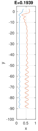
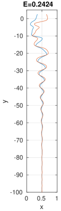
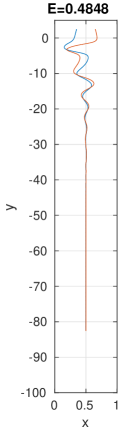
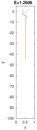
Figure 7: Trajectories of two disks for $\rho_{s}=1.0015$ and different values of E.

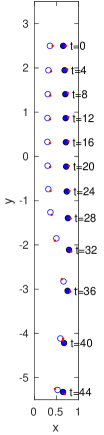
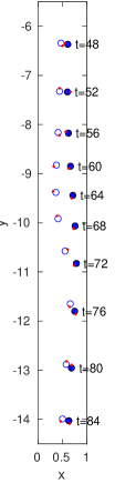
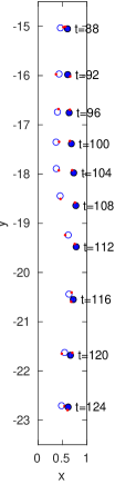
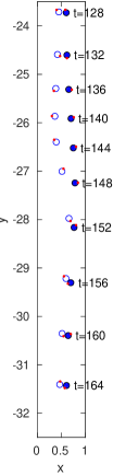
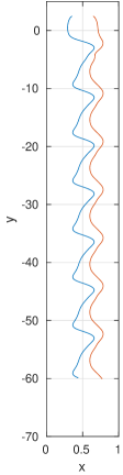
Figure 8: Positions of two disks drafting, kissing, and not-chaining for $\rho_{s}=1.005$ and E=0.4 (the other associate numbers are Re=1.0824, M=0.6846 and De=0.4330).

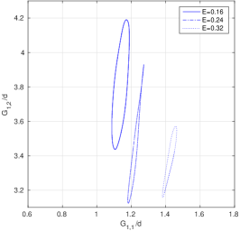
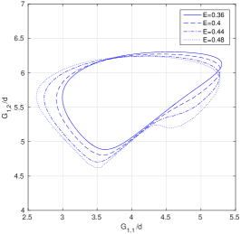
Figure 9: Trajectories of disks in phase space of the normalized distances between the disk mass center and the left wall for $\rho_{s}=1.005$. The periods of two disks interacting apart are 21.65, 18.05 and 16.28 for E=0.16, 0.24 and 0.32, respectively (left) and the periods of two disks drafting, kissing, and not-chaining are 34.2, 38.45, 46.45 and 64 for E=0.36, 0.4, 0.44 and 0.48, respectively (right).

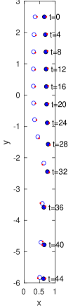
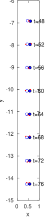
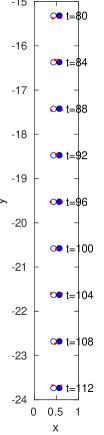
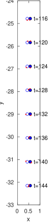
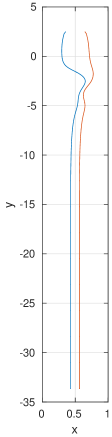
Figure 10: Positions of two disks for $\rho_{s}=1.005$ and E=0.56 (the other associate numbers are Re=1.3150, M=0.9841 and De=0.7364).

For the particles of the density $\rho_{s}$=1.0015, similar particle motions are obtained. For $E\leq 0.2182$, two disks stay separated and interact periodically. This periodic motion between two disks just likes the one in Fig. 3 and its associated limit cycle is similar to those in the left plot in Fig. 5. For E between 0.2424 and 1.0667, the orientation of the disk chain oscillates first and then turns into vertical direction after the oscillation damps out (e.g., see the trajectories of two disks for E=0.2424 and 0.4848 shown in Fig. 7). For E between 1.2606 and 1.6, two disks form a chain and then turn its orientation into the falling direction right away. The tilted chain is not obtained for the values of the elasticity number considered in the phase diagram presented in Fig. 6. The critical value of the elasticity number for having a vertical chain is somewhere in the interval [0.2182, 0.2424].

For the particles of slightly heavier densities $\rho_{s}$= 1.0035 and 1.005, we have also obtained similar kinds of particle motion for various values of the elasticity number as shown together with $\rho_{s}$=1.0015 and 1.0025 in a phase plane in Fig. 6. But the range of the elasticity number for having the tilted chain is wider. Also for these relatively heavier disks, besides the typical periodical motion discussed in the above cases, there is another one which we call “drafting, kissing and not-chaining” (see Fig. 8). The limit cycles of those two types of periodic motion for $\rho_{s}$=1.005 are shown in Fig. 9. The limit cycles in the left plot in Fig. 9 are associated with the motion like the one in Fig. 3 and those in the right plot are associated with the drafting, kissing and not-chaining. The particle positions and trajectories for $\rho_{s}$=1.005 and E=0.4 shown in Fig. 8 tell us that every time a chain is about to be formed after drafting and kissing between two disks, the “long body” of two disks turns and then two disks break away. We believe that this not being able to form a chain between two disks is due to the weak elastic force since, for E=0.56, an almost horizontal and stable chain is formed (see Fig. 10). By comparing the particle position shown in Figs. 8 and 10, we observe that two particles kiss between $t=40$ and $48$ for E=0.4 and 0.56. Then the pair in Fig. 8 breaks up at $t=52$ for the case of E=0.4, but the other pair for E=0.56 remain chained.

All values of the Mach number associated with the different values of the particle density $\rho_{s}$ and elasticity number are presented in Fig. 6. For each fixed value of the elasticity number E, when the particle is heavier, the Mach number is increased. For example, at E=1.6, two disks form a chain and then its orientation turns into the falling direction right away for all four particle densities (see Fig. 11). The associated values of the Mach number of these four cases are 0.6697, 1.0582, 1.4004 and 1.8468 for $\rho_{s}=$1.0015, 1.0025, 1.0035 and 1.005, respectively. As discussed in [6], the long body flips falling broadside-on for Mach number greater than its critical value ($O(1)$). To see the effect of the larger value of the Mach number on the chain orientation, the numerical results of two disks of $\rho_{s}=1.01$ at E= 1.6 do show that a stable tilted particle chain is obtained (see Fig. 12). The tilt angle of the chain is about 32 degrees and the associated Mach number is M= 3.0784. For E=1.44, similar results are also obtained. The tilt angle of the chain is 31.59 degrees and the associated Mach number is M= 2.8660. Hence the values of the elasticity number and the Mach number determine whether the the chain can be formed and the orientation of the chain, which is consistent with the results obtained in [6] for elliptic particles settling Oldroyd-B fluids.

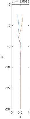
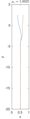
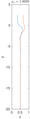
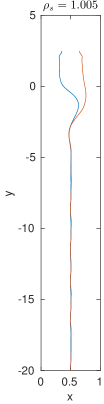
Figure 11: Trajectories of two disks having vertical chain for four different densities and E=1.6.

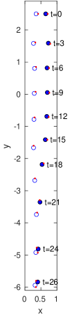
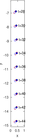
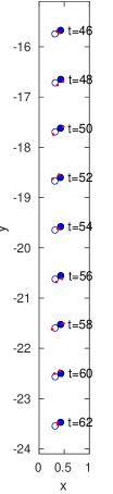
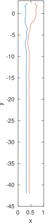
Figure 12: Positions of two disks (left three) and trajectories of two disks (right) for$\rho_{s}=1.01$ and E=1.6 (the other associate numbers are Re=2.4337, M=3.0784 and De=3.8940).

4 Conclusion

In this article we present a numerical study of the dynamics of two disks settling in a narrow vertical channel filled with an Oldroyd-B fluid. For the cases considered in this article, two kinds of particle dynamics are obtained: (i) periodic interaction between two disks and (ii) the formation of the chain of two disks. For the periodic interaction of two disks, two different motions are obtained: (a) two disks stay far apart and their interaction is periodical, which is similar to one of the motions of two disks settling in a narrow channel filled with a Newtonian fluid discussed in [19] and (b) two disks draft, kiss and break away periodically and the chain is not formed due to the lack of strong enough elastic force. For the formation of two disk chain occurred at higher values of the elasticity number, it is either a tilted chain or a vertical chain. The tilted chain can be obtained for either that the elasticity number is less than the critical value for having the vertical chain or that the Mach number is greater than the critical value for a long body to fall broadside-on. Hence the values of the elasticity number and the Mach number determine whether the the chain can be formed and the orientation of the chain.

References

- [1] R. P. Chhabra, Bubbles, Drops, and Particles in Non-Newtonian Fluids, CRC Press, Boca Raton, FA, USA, 1993.
- [2] G. H. McKinley, Steady and transient motion of spherical particles in viscoelastic liquids, in: R.P. Chhabra, D. De Kee (Eds.), Transport Processes in Bubbles, Drops and Particles, 2nd ed., Taylor & Francis, New York, NY, 2002, pp. 338-375.
- [3] M. J. Economides, K. G. Nolte, Reservoir Stimulation. Prentice Hall, Englewood Cliffs, NJ, USA, 1989.
- [4] J. Feng, P.Y. Huang, D.D. Joseph, Dynamic simulation of sedimentation of solid particles in an Oldroyd-B fluid, J. Non-Newtonian Fluid Mech., 63 (1996), 63-88.
- [5] H.H. Hu, N.A. Patankar,M.Y. Zhu, Direct numerical simulations of fluid-solid systems using the arbitrary Lagrangian-Eulerian technique, J. Comput. Phys., 169 (2001), 427-462.
- [6] P. Y. Huang, H. H. Hu, D. D. Joseph, Direct simulation of the sedimentation of elliptic particles in Oldroyd-B fluids, J. Fluid Mech., 362 (1998), 297-325.
- [7] P. Singh, D. D. Joseph, T. I. Helsa, R. Glowinski, T.-W. Pan, A distributed Lagrange multiplier/fictitious domain method for viscoelastic particulate flows, J. Non-Newtonian Fluid Mech., 91 (2000), 165-188.
- [8] X.M. Shao, Z.S. Yu, Sedimentation of circular particles in Oldroyd-B fluid, J. Hydrodynamics, 16 (2004) 254-259.
- [9] J. Hao, T.-W. Pan, R. Glowinski, D. D. Joseph, A fictitious domain/distributed Lagrange multiplier method for the particulate flow of Oldroyd-B fluids: A positive definiteness preserving approach, J. Non-Newtonian Fluid Mech., 156 (2009), 95-111.
- [10] G. D’Avino, P.L. Maffettone, Particle dynamics in viscoelastic liquids J. Non-Newtonian Fluid Mech., 215 (2015), 80–104.
- [11] D.D. Joseph, Y.J. Liu, M. Poletto, J. Feng, Aggregation and dispersion of spheres falling in viscoelastic liquids, J. Non-Newtonian Fluid Mech., 54(1994), 45-86.
- [12] F. P. T. Baaijens, Mixed finite element methods for viscoelastic flow analysis: A review, J. Non-Newtonian Fluid Mech. 79 (1998), 361-385.
- [13] R. Keunings, A survey of computational rheology, in: D. M. Binding et al. (Eds.), Proc. 13th Int. Congr. on Rheology, Vol. 1, British Society of Rheology, Glasgow, United Kingdom, 2000, pp. 7-14.
- [14] R. Fattal, R. Kupferman, Constitutive laws for the matrix-logarithm of the conformation tensor, J. Non-Newtonian Fluid Mech., 123 (2004), 281-285.
- [15] R. Fattal, R. Kupferman, Time-dependent simulation of viscoelastic flows at high Weissenberg number using the log-conformation representation, J. Non-Newtonian Fluid Mech., 126 (2005), 23-37.
- [16] Y.-L. Lee, J. Xu, New formulations, positivity preserving discretizations and stability analysis for non-Newtonian flow models, Comput. Methods Appl. Mech. Eng., 195 (2006), 1180-1206.
- [17] A. Lozinski, R.G. Owens, An energy estimate for the Oldroyd-B model: theory and applications, J. Non-Newtonian Fluid Mech., 112 (2003), 161-176.
- [18] A. F. Fortes, D. D. Joseph, T. S. Lundgren, Nonlinear mechanics of fluidization of beds of spherical particles, J. Fluid Mech., 177 (1987), 467-483.
- [19] C. K. Aidun, E. J. Ding, Dynamics of particle sedimentation in a vertical channel: Period-doubling bifurcation and chaotic state, Phys. Fluids, 15 (2003), 1612-1621.
- [20] D. D. Joseph, Fluid Dynamics of Viscoelastic Liquids, Springer, New York, NY, USA, 1990
- [21] R. Glowinski, T.-W. Pan, T. I. Hesla, D. D. Joseph, J. Périaux, A fictitious domain approach to the direct numerical simulation of incompressible viscous fluid flow past moving rigid bodies: application to particulate flow, J. Comput. Phys., 169 (2001), 363-426.
- [22] R. Glowinski, Finite element methods for incompressible viscous flow, in: P. G. Ciarlet, J.-L. Lions (Eds.), Handbook of Numerical Analysis, Vol. IX, North-Holland, Amsterdam, Netherlands, 2003, pp. 3-1976.
- [23] E. J. Dean, R. Glowinski, A wave equation approach to the numerical solution of the Navier-Stokes equations for incompressible viscous flow, C.R. Acad. Sci. Paris, Série I, t. 325 (1997), 783-791.
- [24] Y. L. Liu, D. D. Joseph, Sedimentation of particles in polymer solutions. J. Fluid Mech., 255 (1993), 565-595.
- [25] H.H. Hu, D. D. Joseph, M. J. Crochet, Direct simulation of fluid particle motions, Theoret. Comput. Fluid Dynamics, 3 (1992), 285-306.
- [26] T.-W. Pan, R. Glowinski, G. P. Galdi, Direct simulation of the motion of a settling ellipsoid in Newtonian fluid, J. Comput. Applied Math., 149 (2002), 71-82.