Static Spherically Symmetric Wormholes in $f(R,T)$ Gravity

Abstract

In this work, we explore wormhole solutions in $f(R,T)$ theory of gravity, where $R$ is the scalar curvature and $T$ is the trace of stress-energy tensor of matter. To investigate this, we consider static spherically symmetric geometry with matter contents as anisotropic, isotropic and barotropic fluids in three separate cases. By taking into account Starobinsky $f(R)$ model , we analyze the behavior of energy conditions for these different kind of fluids. It is shown that the wormhole solutions can be constructed without exotic matter in few regions of spacetime. We also give the graphical illustration of obtained results and discuss the equilibrium picture for anisotropic case only. It is concluded that the wormhole solutions with anisotropic matter are realistic and stable in this gravity.

Keywords: Wormholes; $f(R,T)$ gravity; Energy Conditions.
PACS:

1 Introduction:

After Edwin Hubble s theory of expanding universe, current observations from Supernovae Type Ia and CMBR (Cosmic Microwave Background Radiations) [1], have confirmed the phenomena of accelerated expanding universe. The modified theories are quite useful in present era because these theories can help to explain the possible cosmic expansion history and its related concepts. In this context, $f(R)$ theory is appeared as one of the first and simplest modifications to the Einstein-Hilbert action. This theory has been extensively employed to discuss the dark energy (DE) and mainly the accelerating cosmic expansion [2]. Furthermore, $f(R)$ theory of gravitation provides us the scenarios of early time inflation and late time expansion of the accelerated universe [3]. The discussions about DE and late time cosmic acceleration are also explained in some other modified theories of gravity such as $f(\tau)$ (where “$\tau$” being the torsion) [4], Gauss-Bonnet Gravity [5], Brans-Dicke theory [6] and $f(T,T_{G})$, [7] etc.

Few years ago, Harko et al. [8] introduced a modification to Einstein’s gravity and named it as $f(R,T)$ theory of gravity. This was basically an extension to $f(R)$ gravity obtained by introducing the trace “$T$” of the energy-momentum tensor together with the Ricci scalar “$R$”. Furthermore, they derived corresponding field equations from the coupling of matter and geometry in metric formalism for some specific cases. Recently, Houndjo [9] reconstructed some cosmological models of the form $f(R,T)=f_{1}(R)+f_{2}(T)$, in the presence of auxiliary scalar field with two known examples of scale factor that correspond to an expanding universe. In [10], authors considered cosmological scenarios based on $f(R,T)$ theories of gravity and numerically reconstructed the function $f(R,T)$ for holographic DE model that can reproduce the same expansion history as generated in general relativity (GR). Till present time, different cosmological aspects have been addressed in $f(R,T)$ gravity including reconstructions schemes, anisotropic solutions, energy conditions, thermodynamics, viscous solutions, phase space perturbations and stability, etc. [11].

Wormholes are hypothetical topological features that provide a subway for different space times apart from each other. In 1935, Einstein and Rosen [12] firstly obtained the wormhole solutions known as Lorentzian wormholes or Schwarzchild wormholes. On the basis of nature, wormholes are of two kinds: static wormholes and dynamic wormholes. Normally, an exotic fluid is needed for the formation of static wormholes which violates the NEC in GR. Lobo and Oliveira [13] explained the fact that how wormhole solutions can be formed without violation of energy conditions, $i.e.,$ WEC and NEC, in $f(R)$ theory of gravity. They reconstructed $f(R)$ by considering trace-less fluid and equations of state for some particular shape function, to discuss the evolution of energy conditions.

In [14], the behavior of ordinary matter was studied to check whether it can support wormholes in $f(R)$ theory. For this purpose, WEC and NEC were analyzed in anisotropic, barotropic and isotropic fluids and it was observed that the barotropic fluid satisfies these conditions in some certain regions of the space-time while for the other two fluids, these conditions were violated. So, wormhole solutions can be obtained without exotic matter in few regions of space-time only, without violating the energy conditions which are necessary for the existence of wormhole solutions in GR [15]. Recently, the wormhole geometries are studied in $f(R,T)$ gravity [16] by taking a particular equation of state (EoS) for the matter field into account. They showed that effective stress-energy is responsible for violation of the NEC.

Here, we are interested to find wormhole solutions by introducing additional matter contributions in $f(R)$ model(without involving any form of exotic matter). We analyze the behavior of shape function, WEC and NEC to explore the suitable regions for existence of wormhole solutions using anisotropic, barotropic and isotropic fluids. This paper has following sequence. In section 2, we present a short introduction of $f(R,T)$ gravity by developing the field equations. Section 3 relates to the discussion of wormhole geometries in $f(R,T)$ theory of gravity for three types of fluids. Finally, section 4 comprises of concluding remarks.

2 $f(R,T)$ Gravity

Here, we will give a short introduction to $f(R,T)$ theory of gravity. In his pioneer work, Harko et al. presented a new generalization of $f(R)$ gravity by taking a coupling of Ricci scalar with matter field into account as follows [8]

$$\mathcal{I}=\int{dx^{4}\sqrt{-g}\left[f(R,T)+\mathcal{L}_{\mathrm{m}}\right]}.$$ (1)

In above action, $f(R,T)$ represents a generic function of Ricci scalar $R$ and the energy-momentum tensor trace $T=T^{\mu}_{\mu}$. Here, in the action, we have assumed the gravitational units, i.e., $c=8\pi{G}=1$ and also matter ingredients are introduced by the Lagrangian density $\mathcal{L}_{(matter)}$. This theory is considered as more successful as compared to $f(R)$ gravity in the sense that such theory can include quantum effects or imperfect fluids that are neglected in simple $f(R)$ generalization of GR. The metric $g_{\mu\nu}$ variation of the above action leads to the following set of field equations:

$$R_{{\mu}{\nu}}f_{R}(R,T) - \frac{1}{2}g_{{\mu}{\nu}}f(R,T)+\big{(}g_{{\mu}{\nu}}{\Box}-{\nabla}_{\mu}{\nabla}_{\nu}\big{)}f_{R}(R,T)$$ (2)

$$= T_{{\mu}{\nu}}-f_{T}(R,T)\Theta_{{\mu}{\nu}}-f_{T}(R,T)T_{{\mu}{\nu}}.$$

This set involves derivative operators like $\nabla$ and $\Box$ that represent covariant derivative and four-dimensional Levi-Civita covariant derivative also known as d’Alembert operator, respectively. Also, the notations $f_{R}(R,T)$ and $f_{T}(R,T)$ correspond to derivatives of $f(R,T)$ with respect to Ricci scalar, i.e., $\frac{\partial{f(R,T)}}{\partial{R}}$ and energy-momentum, i.e., trace $\frac{\partial{f(R,T)}}{\partial{T}}$, respectively. The term $\Theta_{{\mu}{\nu}}$ is defined by

$$\Theta_{{\mu}{\nu}}=\frac{g^{\alpha{\beta}}{\delta}T_{{\alpha}{\beta}}}{{\delta}g^{\mu{\nu}}}=-2T_{{\mu}{\nu}}+g_{\mu\nu}\mathcal{L}_{m}-2g^{\alpha\beta}\frac{\partial^{2}\mathcal{L}_{m}}{{\partial}g^{\mu\nu}{\partial}g^{\alpha\beta}},$$

where the matter energy-momentum tensor is introduced which is given by the following equation [17]

$$T_{{\mu}{\nu}}^{(m)}=-\frac{2}{\sqrt{-g}}\frac{\delta(\sqrt{-g}{\mathcal{\mathcal{L}}_{m}})}{\delta{g^{{\mu}{\nu}}}}=g_{{\mu}{\nu}}\mathcal{L}_{m}-\frac{2{\partial}{\mathcal{L}_{m}}}{\partial{g^{{\mu}{\nu}}}}.$$ (3)

Here the second part of the above equation can be obtained, if the matter Lagrangian is assumed to depend only on the metric tensor rather than on its derivatives.

The source of anisotropic fluid is defined by the following energy momentum tensor

$$T_{{\mu}{\nu}}=({\rho}+p_{r})V_{\mu}V_{\nu}-p_{t}g_{{\mu}{\nu}}+(p_{r}-p_{t})\chi_{\mu}\chi_{\nu},$$

where $V_{\mu}$ is the 4-velocity of the fluid defined as $V^{\mu}=e^{-a}\delta^{\mu}_{0}$ satisfying $V^{\mu}V_{\mu}=1$ and $\chi^{\mu}=e^{-b}\delta^{\mu}_{1}$ gives $\chi^{\mu}\chi_{\mu}=-1$. Herein, we choose $\mathcal{L}_{(matter)}={\rho}$, then the expression for $\Theta_{{\mu}{\nu}}$ takes the following form

$$\Theta_{{\mu}{\nu}}=-2T_{{\mu}{\nu}}+{\rho}g_{{\mu}{\nu}}.$$

Consequently, the field equations (2) can be expressed as effective Einstein field equations of the form

$$R_{{\mu}{\nu}}-\frac{1}{2}Rg_{{\mu}{\nu}}=T_{{\mu}{\nu}}^{eff},$$ (4)

where $T_{{\mu}{\nu}}^{eff}$ is the effective energy-momentum tensor in $f(R,T)$ gravity which is defined by

$${T}_{{\mu}{\nu}}^{eff} = \frac{1}{f_{R}(R,T)}\left[(1+f_{T}(R,T))T_{\mu\nu}-\rho g_{\mu\nu}f_{T}(R,T)+\frac{1}{2}(f(R,T)\right.$$ (5)

$$- \left.Rf_{R}(R,T))g_{\mu\nu}+({\nabla}_{\mu}{\nabla}_{\nu}-g_{{\mu}{\nu}}{\Box})f_{R}(R,T)\right].$$

3 Wormhole Geometries with Three Different Matter Contents

In this section, we will discuss static spherically symmetric wormholes with three types of matter contents: anisotropic, isotropic and barotropic. Consider a line element that describes static spherically symmetric geometry of the form

$$ds^{2}=e^{a(r)}dt^{2}-e^{b(r)}dr^{2}-r^{2}(d\theta^{2}+sin^{2}\theta d\phi^{2}),$$ (6)

where $a(r)$ is an arbitrary function of $r$ and for the wormhole geometry, we have $e^{-b(r)}=1-\beta(r)/r$. The terms $a(r)$ and $\beta(r)$ represent the redshift function, and the shape function, respectively [15]. For the surface vertical to the wormhole throat, we must have a minimum radius at $r=\beta(r_{0})=r_{0}$, then it increases from $r_{0}$ to $r\rightarrow\infty$. An important condition to have a typical wormhole solution is the flaring out condition of the throat, given by $\frac{(\beta-\beta^{\prime}r)}{\beta^{2}}>0$ and moreover, $\beta(r)$ needs to meet the condition $\beta^{\prime}(r_{0})<1$ that is imposed at the throat $\beta(r_{0})=r=r_{0}$. In GR, these conditions hints the existence of exotic form of matter which requires the violation of the NEC. Also, the condition $1-\beta(r)/r>0$ needs to be satisfied.

The field equations can be rearranged to find the expressions for $\rho$, $p_{r}$ and $p_{t}$ as follows

$$\rho = \frac{1}{e^{b}}\left[\bigg{(}\frac{a^{\prime}}{r}-\frac{a^{\prime}b^{\prime}}{4}+\frac{a^{\prime\prime}}{2}+\frac{a^{\prime 2}}{4}\bigg{)}f_{R}(R,T)+\bigg{(}\frac{b^{\prime}}{2}-\frac{2}{r}\bigg{)}f^{\prime}_{R}(R,T)-f^{\prime\prime}_{R}(R,T)\right.$$ (7)

$$- \left.\frac{f(R,T)}{2}e^{b}\right],$$

$$p_{r} = \frac{1}{e^{b}(1+f_{T}(R,T))}\left[\bigg{(}\frac{b^{\prime}}{r}-\frac{a^{\prime}b^{\prime}}{4}-\frac{a^{\prime\prime}}{2}-\frac{a^{\prime 2}}{4}\bigg{)}f_{R}(R,T)+\bigg{(}\frac{a^{\prime}}{2}+\frac{2}{r}\bigg{)}f^{\prime}_{R}(R,T)\right.$$ (8)

$$\left.+\frac{f(R,T)}{2}e^{b}\right]-\frac{{\rho}f_{T}(R,T)}{(1+f_{T}(R,T))},$$

$$p_{t} = \frac{1}{e^{b}(1+f_{T}(R,T))}\left[\bigg{(}\frac{(b^{\prime}-a^{\prime})r}{2}-e^{b}+1\bigg{)}\frac{f_{R}(R,T)}{r^{2}}+\bigg{(}\frac{a^{\prime}-b^{\prime}}{2}+\frac{1}{r}\bigg{)}f^{\prime}_{R}(R,T)\right.$$ (9)

$$\left.+f^{\prime\prime}_{R}(R,T)+\frac{f(R,T)}{2}e^{b(r)}\right]-\frac{{\rho}f_{T}(R,T)}{(1+f_{T}(R,T))}.$$

It can be observed that the above equations appeared as much complicated to find the explicit expressions of $\rho$, $p_{r}$ and $p_{t}$, since $f(R,T)$ has direct dependence on trace of stress-energy tensor. In this scenario, we find that the only possibility left is to choose the function as $f(R,T)=f(R)+f(T)$ with $f(T)=\lambda T$, where $\lambda$ being the coupling parameter. Here, we set this choice for $f(R,T)$ and simplify the above equations (7)-(9) as follows

$$\rho = \frac{1}{2(1+2{\lambda})}\bigg{[}\frac{2+5{\lambda}}{(1+{\lambda})}Z_{1}+{\lambda}Z_{2}+2{\lambda}Z_{3}\bigg{]},$$ (10)

$$p_{r} = \frac{-1}{2(1+2{\lambda})}\bigg{[}\frac{{\lambda}}{(1+{\lambda})}Z_{1}-(2+3{\lambda})Z_{2}+2{\lambda}Z_{3}\bigg{]},$$ (11)

$$p_{t} = \frac{-1}{2(1+2{\lambda})}\bigg{[}\frac{{\lambda}}{(1+{\lambda})}Z_{1}-(2+3{\lambda})Z_{2}+2{\lambda}Z_{3}\bigg{]},$$ (12)

where

$$Z_{1} = \frac{1}{e^{b}}\bigg{[}\bigg{(}\frac{a^{\prime}}{r}-\frac{a^{\prime}b^{\prime}}{4}+\frac{a^{\prime\prime}}{2}+\frac{a^{\prime 2}}{4}\bigg{)}f_{R}+\bigg{(}\frac{b^{\prime}}{2}-\frac{2}{r}\bigg{)}f^{\prime}_{R}-f^{\prime\prime}_{R}-\frac{f}{2}e^{b}\bigg{]},$$

$$Z_{2} = \frac{1}{e^{b}(1+{\lambda})}\bigg{[}\bigg{(}\frac{b^{\prime}}{r}+\frac{a^{\prime}b^{\prime}}{4}-\frac{a^{\prime\prime}}{2}-\frac{a^{\prime 2}}{4}\bigg{)}f_{R}+\bigg{(}\frac{a^{\prime}}{2}+\frac{2}{r}\bigg{)}f^{\prime}_{R}+\frac{f}{2}e^{b}\bigg{]},$$

$$Z_{3} = \frac{1}{e^{b}(1+{\lambda})}\bigg{[}\bigg{(}\frac{(a^{\prime}-b^{\prime})r}{2}-e^{b}+1\bigg{)}\frac{-f_{R}}{r^{2}}+\bigg{(}\frac{a^{\prime}-b^{\prime}}{2}+\frac{1}{r}\bigg{)}f^{\prime}_{R}$$

$$+f^{\prime\prime}_{R}+\frac{f}{2}e^{b}\bigg{]}.$$

In [18], authors have presented the study of energy conditions in $f(R,T)$ gravity. We recommend the readers to see these papers for having an overview of this subject. As for the other modified theories, the violation of the NEC in $f(R,T)$ gravity imposes the condition $T_{\mu\nu}^{eff}\kappa^{\mu}\kappa^{\nu}<0$, that is, $\rho^{eff}+p^{eff}<0$. Here, we find the following expression:

$$\rho^{eff}+p_{r}^{eff}=\frac{1}{f_{R}}(\rho+p_{r})(1+\lambda)+\frac{1}{f_{R}}\left(1-\frac{\beta}{r}\right)\left(f^{\prime\prime}_{RR}+f^{\prime}_{R}\frac{\beta-\beta^{\prime}r}{2r^{2}(1-\frac{\beta}{r})}\right).$$

Using the field equations, this leads to

$$\rho^{eff}+p_{r}^{eff}=\frac{1}{r^{3}}\bigg{(}{\beta}^{\prime}r-\beta\bigg{)},$$

which is similar to that in $f(R)$ gravity. Here, if we use the flaring out condition $\frac{(\beta-\beta^{\prime}r)}{\beta^{2}}>0$, it results in $\rho^{eff}+p^{eff}<0$. In this case, we have kept NEC satisfied for matter energy tensor, however the additional curvature components which arise due to modification of Einstein’s gravity play role for violation of the NEC.

In this study, we take a specific $f(R)$ model representing $R^{n}$ extension of well known Starobinsky model [3] and is given by [19]

$$f(R)=R+\alpha R^{2}+\gamma R^{n},$$

where $n\geqslant 3$, $\alpha$ and $\gamma$ are arbitrary constants. The choice of $\alpha=\gamma=0$ implies the $\Lambda$ correction to GR. Basically, we want to take power law model that should be singularity free as well as it should be the generalization of linear models that are used in most of the literature for wormhole discussions. In literature [20], it is pointed out that the power law models are always of great interest, e.g., $f(R)=\xi R^{n}$ with $\xi,n$ are any constants. In this model, there exists big rip singularities for negative range of $n$. They also argued that if we impose $n>1$ with positive $\xi$, then $f(R)\rightarrow\infty$ only when $R\rightarrow\infty$. Thus under these conditions, the possible presence of singularity can be avoided. Further, in literature, another form of Starobinsky model with disappearing cosmological constant is defined $f(R)=R+\lambda R_{0}[(1+\frac{R^{2}}{R_{0}})^{-n}-1]$. Clearly, this model suffers the singularity problem. However, they also claimed that this singularity can be cured by adding a term $\propto R^{2}$ [21]. It can be easily seen that our used Starobinsky model has different form involving one $R^{2}$ term, therefore our used model does not suffer with any singularity problem. One can explore another viable $f(R)$ model named as Hu-Sawicki model to present interesting cosmic features [22].

For this model, the field equations (10)-(12) take the form

$$\rho = \frac{e^{-b}}{4r^{2}(1+{\lambda})(1+2{\lambda})}\bigg{[}(1+2{\alpha}R+n{\gamma}R^{n-1})(2r^{2}{a^{\prime\prime}}(1+2{\lambda})-{a^{\prime}}r(1+2{\lambda})$$ (13)

$$\times \big{(}r{b^{\prime}}-4)+r^{2}{a^{\prime}}^{2}(1+{\lambda})+4r{b^{\prime}}{\lambda}+4{\lambda}(e^{b}-1))+(2{\alpha}+n(n-1){\gamma}R^{n-2})$$

$$\times \big{(}3r^{2}{a^{\prime}}{\lambda}+r(2+3{\lambda})(r{b^{\prime}}-4)R^{\prime}-2r^{2}{R}e^{b}(1+{\lambda})(R+{\alpha}R^{2}+{\gamma}R^{n})-2r^{2}$$

$$\times \big{(}2+3{\lambda})({\gamma}n(n-1)(n-2)R^{n-3}R^{\prime 2}+2{\alpha}R^{\prime\prime}+{\gamma}n(n-1)R^{n-2}R^{\prime\prime}\bigg{]},$$

$$p_{r} = \frac{e^{-b}}{4r^{2}(1+\lambda)(1+2\lambda)}\bigg{[}\big{(}1+2\alpha R+n\gamma R^{n-1}\big{)}\big{(}-4\big{(}-1+e^{b}\big{)}\lambda+r\big{(}$$ (14)

$$- (r+2r\lambda)a^{\prime 2}+4(1+\lambda)b^{\prime}+r(1+2\lambda)a^{\prime}b^{\prime}-2r(1+2\lambda)a^{\prime\prime}\big{)}\big{)}+r\big{(}\big{(}2\alpha$$

$$+ n(n-1)\gamma R^{n-2}\big{)}\big{(}8+12\lambda+r(2+\lambda)a^{\prime}+r\lambda b^{\prime}\big{)}R^{\prime}+2r\big{(}e^{b}(1+\lambda)\big{(}R$$

$$+ \alpha R^{2}+\gamma R^{n}\big{)}-2\alpha\lambda R^{\prime\prime}-n(n-1)\gamma\lambda R^{n-3}\big{(}(n-2)R^{\prime 2}+RR^{\prime\prime}\big{)}\big{)}\big{)}\bigg{]},$$

$$p_{t} = \frac{e^{-b}}{4r^{2}\big{(}1+3\lambda+2\lambda^{2}\big{)}}\bigg{[}2\big{(}1+2\alpha R+n\gamma R^{n-1}\big{)}\big{(}2\big{(}e^{b}-1\big{)}(1+\lambda)$$ (15)

$$- (r+2r\lambda)a^{\prime}+rb^{\prime}\big{)}+r\big{(}\big{(}2\alpha+n(n-1)\gamma R^{n-2}\big{)}\big{(}4(1+\lambda)+r(2+\lambda)a^{\prime}$$

$$- r(2+3\lambda)b^{\prime}\big{)}R^{\prime}+2r\big{(}e^{b}(1+\lambda)\big{(}R+\alpha R^{2}+\gamma R^{n}\big{)}+(2+3\lambda)\big{(}n(n-1)$$

$$\times (n-2)\gamma R^{n-3}R^{\prime 2}+2\alpha R^{\prime\prime}+n(n-1)\gamma R^{n-2}R^{\prime\prime}\big{)}\big{)}\big{)}\bigg{]}.$$

In further discussion, we take a particular value for $n$ as $n=3$. Moreover, the redshift function is chosen to be constant with $a^{\prime}(r)=0$. In coming sections, we discuss the energy bounds for three different fluid configurations.

3.1 Anisotropic fluid

Initially, we consider the anisotropic fluid model with the following choice of shape function [23]-[26]

$$b(r)=-\text{ln}\bigg{[}1-\bigg{(}\frac{r_{0}}{r}\bigg{)}^{m+1}\bigg{]},$$ (16)

where $m$ and $r_{0}$ are arbitrary constants. Since $e^{-b(r)}=1-\beta(r)/r$, so, in our case, Eq.(16) implies the following form of shape function

$$\beta(r)=\frac{(r_{0})^{m+1}}{r^{m}}.$$ (17)

Clearly, $\beta(r)$ is characterized on the basis of $m$ and can result in different forms, which have been explored in literature as shown in Table 1. Here, $\beta(r)$ satisfies the necessary conditions for the existence of shape function. To meet the flaring out condition $\beta^{\prime}(r)<1$, one need to set $m<1$. Also, the constraint $\beta(r_{0})=r_{0}$ is trivially satisfied. Moreover, this shape function also satisfies the condition for asymptotically flat spacetime, i.e., $\beta(r)/r=r_{0}^{1-m}r^{m-1}\rightarrow 0$ as $r\rightarrow\infty$.

$m$	$m=1$	$m=1/2$	$m=1/5$	$m=0$	$m=-1/2$	$m=-3$
Shape Functions $\beta(r)$	$r_{0}^{2}/r$	$r_{0}\sqrt{r_{0}/r}$	$r_{0}^{6/5}r^{-1/5}$	$r_{0}$	$\sqrt{r_{0}r}$	$r_{0}^{2}r^{3}$

Table 1: Shape functions corresponding to different choices of parameter $m$.

In [14], Lobo and Oliveira discussed the wormhole geometries in $f(R)$ gravity using the above defined shape function for the choices: $m=1$ and $m=-1/2$. Recently, Pavlovic and Sossich [25] discussed the existence of wormholes without exotic matter in different $f(R)$ models employing this shape function (16) with $m=1/2$.

Substituting $b(r)$ in Eqs. (13)-(15), we obtain

$$\rho = \frac{r_{0}m}{r^{9}(1+\lambda)(1+2\lambda)}\left(\frac{r_{0}}{r}\right)^{m}\bigg{[}-r^{4}\bigg{(}r^{2}(1+2\lambda)+2(2+m)(3+m)\alpha(2+3\lambda)\bigg{)}$$ (18)

$$+ r_{0}\left(\frac{r_{0}}{r}\right)^{m}r\bigg{(}-12m(3+m)(5+2m)\gamma(2+3\lambda)+r^{2}\alpha\bigg{(}30+26m+6m^{2}+45\lambda$$

$$+ 9m\lambda(4+m)\bigg{)}\bigg{)}+2\gamma r_{0}^{2}m\big{(}\frac{r_{0}}{r}\big{)}^{2m}\bigg{(}m(154+226\lambda)+(15m^{2}+99)$$

$$\times (2+3\lambda)\bigg{)}\bigg{]},$$

$$p_{r} = \frac{r_{0}}{r^{9}(1+\lambda)(1+2\lambda)}\left(\frac{r_{0}}{r}\right)^{m}\bigg{[}-r^{4}\bigg{(}r^{2}(1+2\lambda)+2m\alpha(3+m)(4+10\lambda+m\lambda)\bigg{)}$$

$$+ 2r_{0}^{2}m^{2}\left(\frac{r_{0}}{r}\right)^{2m}\gamma\bigg{(}33(2+7\lambda)+m(20+(122+15m)\lambda)\bigg{)}+r_{0}m\left(\frac{r_{0}}{r}\right)^{m}r\bigg{(}-12m\gamma$$ (19)

$$\times (3+m)(4+(13+2m)\lambda)+r^{2}\alpha\bigg{(}20+55\lambda+m(6+(28+3m)\lambda)\bigg{)}\bigg{)}\bigg{]},$$

$$p_{t} = \frac{r_{0}}{2r^{9}(1+\lambda)(1+2\lambda)}\left(\frac{r_{0}}{r}\right)^{m}\bigg{[}-4r_{0}^{2}m^{2}\left(\frac{r_{0}}{r}\right)^{2m}\gamma\bigg{(}231+169m+30m^{2}+(3+m)$$ (20)

$$\times (121+45m)\lambda\bigg{)}+r^{4}\bigg{(}(1+m)r^{2}(1+2\lambda)+4m(3+m)\alpha(6+10\lambda+m(2$$

$$+ 3\lambda))\bigg{)}+2r_{0}m\left(\frac{r_{0}}{r}\right)^{m}r\bigg{(}-r^{2}\alpha\bigg{(}40+65\lambda+m(16+3m)(2+3\lambda)\bigg{)}$$

$$+ 12m\gamma(3+m)\bigg{(}12+19\lambda+m(4+6\lambda)\bigg{)}\bigg{)}\bigg{]}.$$

In the following discussion, we present the suitable choice of parameters for the viability of WEC: $\rho>0$ and NECs: $\rho+p_{r}>0$, $\rho+p_{t}>0$. We compare the different shape functions depending on the choice of parameter $m$.

• $\beta(r)=r_{0}\sqrt{\frac{r_{0}}{r}}$

Here, we fix $r_{0}=1$ and $m=1/2$ and discuss the viability ranges of $\alpha$, $\gamma$ and $r$ for two cases of coupling constant, $\lambda>-1$ and $\lambda<-1$. In case of WEC, we find the following constraints:

• For $\lambda<-1$, WEC is valid if $r\geq 3$ and $\alpha\geq 15$, here $r$ depends on the choice of $\alpha$, for very large $\alpha$, we can increase the validity region. However, $r$ obeys the initial bound $r\geq 1.3$ for greater values of $\alpha$. In left plot of the Fig. 1, we show the evolution of WEC versus $\alpha$, $\gamma$ and $r$ for $\lambda=-2$. One can see that there are some small regions where WEC is also valid for $\alpha<0$. For small choice of $r$, we refer the readers to see the right plot in Fig. 1. We have shown the plot for $\lambda=-2$, it can be seen that there some small regions of validity involving $\alpha<0$ and very small range of $r$.

  • For small region like $0<r\leq 1$, we require $\gamma\leq-30$ and for $1<r<3$, we require $\alpha>0$ with $\gamma\geq 30$.

• For $\lambda>-1$, the validity of WEC needs $\alpha\leq-20$ and $r\geq 2.8$. In left plot of Fig. 2, we have shown the validity regions for $\lambda=2$, it can be seen that there some small regions of validity involving $\alpha>0$ and very small range of $r$. In right plot of Fig. 2, we show the evolution for small ranges of $r$ and find the following constraints:

  • For small region like $0<r<1$, we require $\gamma\geq 20$ and for $1.2\leq r<2.8$, the validity needs negative values of both $\alpha$ and $\gamma$.

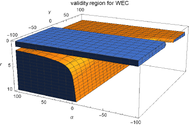
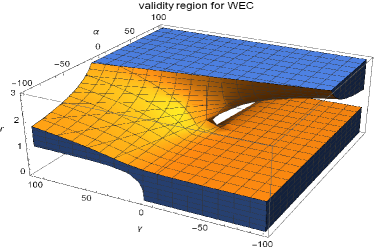
Figure 1: Validity of WEC for $\lambda=-2$ with $c=1$ and $m=1/2$. In right plot, we present the evolution for small $r$ which is as clear in left plot.

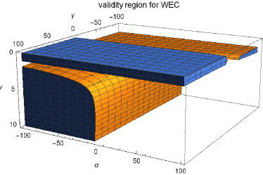
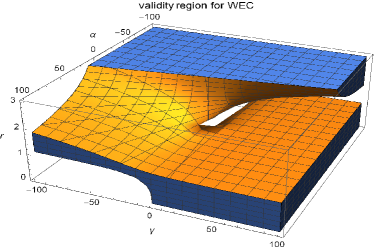
Figure 2: Validity of WEC for $\lambda=-2$ with $c=1$ and $m=1/2$. In right plot, we present the evolution for small $r$ which is as clear in left plot.

Now we discuss the validity regions for $\rho+p_{r}>0$ and $\rho+p_{t}>0$. Again we develop two cases depending on the choice of $\lambda$.

• For $\lambda<-1$, $\rho+p_{r}>0$ is valid in following regions:
  $0<r<1$ with $\gamma\leq-13$; $r\geq 1.1$ with $\alpha>0$ and $\gamma>-1$; $r\geq 3$ with $\alpha\geq 10$.

• The validity of $\rho+p_{t}>0$ can be met for three cases, i.e.,
  $0<r<1$ with $\gamma\geq 15$; $r\geq 1.1$ with $\alpha\leq-10$, and $\gamma<0$; if $r\geq 3$ with $\alpha\leq-10$.

Now we present the constraints for $\lambda>-1$.

• Here, $\rho+p_{r}>0$ can be satisfied for four different ranges depending on the choice of $r$: if $0<r<1$ with $\gamma\geq 15$; if $r\geq 2.9$, $\alpha\leq-15$; if $1<r<2.9$, $\alpha<0$, $\gamma<0$ and if $r\geq 1.1$ with $\gamma<0$ and $\alpha\leq-10$.

• In case of $\rho+p_{t}>0$, we can find the validity for the following choices of the parameters: For $0<r<1$ with $\gamma\leq-16$; for $r\geq 2.9$ with $\alpha\geq 10$; for $1\leq r<2.9$ with $\alpha>0$, $\gamma>0$ and for $r\geq 1.1$ with $(\alpha,\gamma)>0$.

In Figs. 3 and 4, we present the evolution of $\rho+p_{r}>0$ and $\rho+p_{t}>0$ for $\lambda=2$ and $\lambda=-2$, respectively. We find that there is no region of similarity between $\rho+p_{r}>0$ and $\rho+p_{t}>0$, though one can find the same validity range for both $\rho>0$ and $\rho+p_{r}>0$. In Fig. 5, we show the plots of the $\rho$, $p_{r}$ and $p_{t}$ for $c=1$, $n=0.5$, $\lambda=2$, $\alpha=-2$ and $\gamma=-0.1$. It can be seen that both $\rho>0$ and $p_{r}>0$ are satisfied but $p_{t}>0$ is violated. Thus, in anisotropic case, the normal matter threading the wormhole does not satisfy $\rho+p_{t}>0$.

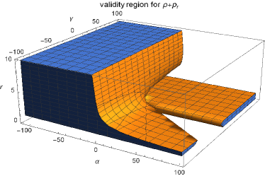
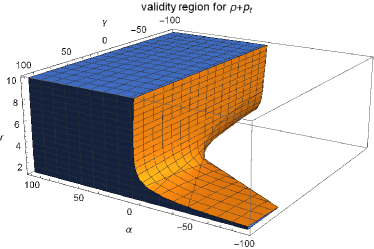
Figure 3: Validity of $\rho+p_{r}>0$ and $\rho+p_{t}>0$ for $\lambda=2$ with $c=1$ and $m=1/2$.

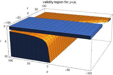
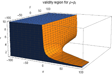
Figure 4: Validity of $\rho+p_{r}>0$ and $\rho+p_{t}>0$ for $\lambda=-2$ with $c=1$ and $m=1/2$.

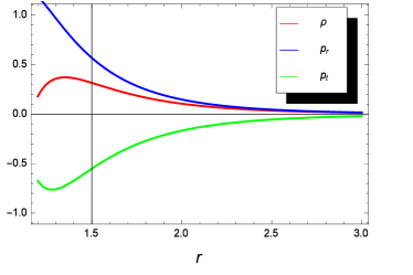
Figure 5: Evolution of $\rho$, $p_{r}$ and $p_{t}$ for the anisotropic case with $\lambda=2$.

• $\beta(r)=r_{0}^{2}/r$

For this choice of shape function, one has to set $m=1$. The results for this choice are very similar as the inequalities remain the same, with only difference with the bounds of parameters.

• For $\lambda<-1$, WEC is valid if $r\geq 3$ and $\alpha\geq 20$. For small region like $0<r\leq 1$, we require $\gamma\leq-10$ and for $1<r<3$, we require $\alpha>0$ with $\gamma\geq 10$. $\rho+p_{r}>0$ is valid in following regions:
  $0<r<1$ with $\gamma\leq-15$; $r\geq 1.1$ with $\alpha>0$ and $\gamma>0$; $r\geq 3$ with $\alpha\geq 15$.
  The validity of $\rho+p_{t}>0$ can be met for three cases, i.e.,
  $0<r<1$ with $\gamma\geq 15$; $r\geq 1.1$ with $\alpha\leq-5$, and $\gamma<0$; if $r\geq 3$ with $\alpha\leq-15$.

• For $\lambda>-1$, the validity of WEC needs $\alpha\leq-20$ and $r\geq 3$. For small region like $0<r<1$, we require $\gamma\geq 10$ and for $1.1\leq r<3$, the validity needs negative values of both $\alpha$ and $\gamma$, i.e, $\alpha\leq-5$ and $\gamma\leq-20$. NEC with radial pressure can be satisfied for the following ranges depending on the choice of $r$: if $0<r<1$ with $\gamma\geq 15$; if $r\geq 3$, $\alpha\leq-15$; if $1<r<3$, $\alpha<-5$, $\gamma<0$.

  In case of $\rho+p_{t}>0$, we can find the validity for the following choices of the parameters: For $0<r<1$ with $\gamma\leq-16$; for $r\geq 3$ with $\alpha\geq 10$; for $1\leq r<3$ with $\alpha>0$, $\gamma>0$.

We would like to mention here that all the choices like $m=1,1/2,-1/2,1/5$ [23]-[26], implies the same sort of results as presented in detail for the case of $m=1/2$. However, the parameter $m=-3$ gives significantly different results.

• $\beta(r)=r_{0}^{2}r^{3}$

For $m=-3$, we find the shape function of the form $\beta(r)=r_{0}^{2}r^{3}$, in this case $\rho$, $p_{r}$ and $p_{t}$ appears to be independent of $r$. Here, the choice of $\lambda<-1$ results in following constraints: WEC, $\rho+p_{r}>0$ and $\rho+p_{t}>0$ are valid only if $\gamma\leq-20$ for all values of $\alpha$. If one sets $\lambda>-1$ then the energy conditions are valid only if $\gamma\geq 15$ for all values of $\alpha$. Hence, for this choice the normal matter threading the wormhole is on cards.

3.2 Equilibrium Condition

Now we present some discussion about the equilibrium picture of wormhole solutions. For wormhole solutions, the equilibrium picture can be discussed by taking Tolman-Oppenheimer-Volkov equation given by:

$$\frac{dp_{r}}{dr}+\frac{\sigma^{\prime}}{2}(\rho+p_{r})+\frac{2}{r}(p_{r}-p_{t})=0,$$ (21)

that is defined for the metric:

$$ds^{2}=e^{\sigma(r)}dt^{2}-e^{b}dr^{2}-r^{2}(d\theta^{2}+\sin^{2}\theta d\phi^{2}),$$

where $\sigma(r)=2a(r)$. This equation describes the equilibrium picture by considering anisotropic force arising from anisotropic matter, hydrostatic and gravitational forces that are identified as follows

$$F_{gf}=-\frac{\sigma^{\prime}(\sigma+p_{r})}{2},\quad F_{hf}=-\frac{dp_{r}}{dr},\quad F_{af}=2\frac{(p_{t}-p_{r})}{r},$$

and the equilibrium equation takes the form:

$$F_{hf}+F_{gf}+F_{af}=0.$$

In our case, since we have taken $a^{\prime}(r)=0$, therefore $F_{gf}$ turns out to be zero and hence the previous equation takes the form:

$$F_{hf}+F_{af}=0.$$

In our case, these forces takes the following form:

$$F_{hf} = \frac{7}{2}r^{-9/2}+(\frac{11}{2})(\frac{59.5}{3})\alpha r^{-13/2}-\frac{21}{12}(515.5\gamma)r^{-23/2}+\frac{3}{2}(504\gamma)r^{-10}$$ (22)

$$- \frac{7}{6}(116.5\alpha)r^{-8},$$

$$F_{af} = \frac{2}{r}[\frac{681.5\gamma}{6}r^{-21/2}-\frac{4.5}{6}r^{-7/2}-\frac{112\alpha}{6}r^{-11/2}+\frac{125\alpha}{6}r^{-7}-\frac{630\gamma}{6}r^{-9}-r^{-7/2}$$ (23)

$$- \frac{59.5\alpha}{3}r^{-11/2}+\frac{515.5\gamma}{6}r^{-21/2}-\frac{1}{6}r^{-9}(504\gamma-116.5\alpha r^{2})],$$

where we have used Eqs.(3.1), (19) and (20) with $m=1/2,~{}n=3,~{}c=1$ and $\lambda=-2$. For the second case, i.e, $\lambda=2$, these forces are given by:

$$F_{hf} = -\frac{35}{42}r^{-9/2}-\frac{11}{42}(87.5\alpha)r^{-13/2}+\frac{21}{84}(667.5\gamma)r^{-23/2}-\frac{672}{2}(9\gamma)r^{-10}$$ (24)

$$+ \frac{7}{2}(162.5)r^{-8},$$

$$F_{af} = \frac{2}{r}[-\frac{1}{30}(1327.5\gamma)r^{-21/2}+\frac{7.5}{30}r^{-7/2}+\frac{210\alpha}{30}r^{-11/2}-\frac{240\alpha}{30}r^{-7}+\frac{1218\gamma}{30}r^{-9}$$ (25)

$$+ \frac{5}{21}r^{-7/2}+\frac{87.5\alpha}{21}r^{-11/2}-\frac{667.5\gamma}{42}r^{-21/2}+\frac{672\gamma}{42}r^{-9}-\frac{162.5\alpha}{42}r^{-7}].$$

The graphical behavior of these forces is given in Fig. 6. Here we have taken $\alpha=15$ and $\gamma=30$ for which WEC is compatible as discussed previously. The right plot corresponds to the case $\lambda=2$, while left plot corresponds to $\lambda=-2$. It can be seen that both these forces show similar behavior but their behaviors are in opposite direction. Therefore, these forces can cancel each other’s effect and hence leads to the stability of total configuration. Thus we can conclude that in case of $f(R,T)$ gravity with anisotropic matter, the wormhole solutions remain stable.

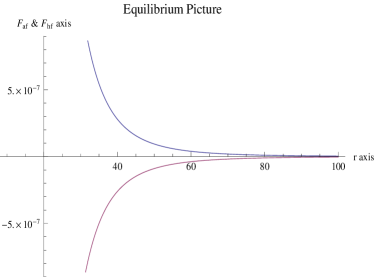
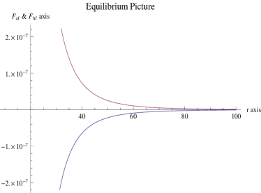
Figure 6: Evolution of $F_{af}$ and $F_{hf}$ versus $r$. Herein, we choose $m=1/2,~{}c=1,~{}n=3,~{}\alpha=15$ and $\gamma=30$. The right and left plots correspond to $\lambda=2$ and $\lambda=-2$, respectively.

3.3 Isotropic fluid

For this case, we consider $p_{r}=p_{t}=p$. Hence, the isotropic condition results in following equation

$$\frac{1}{r(1+\lambda)}e^{-b}\bigg{[}-12r^{3}\bigg{(}e^{b}\big{(}r^{2}\alpha-6\gamma\big{)}-\gamma\bigg{)}b^{\prime 3}+120r^{4}\gamma b^{\prime 4}-12r^{2}b^{\prime 2}\bigg{(}e^{b}$$ (26)

$$\times \bigg{(}r^{2}\alpha-28\gamma\bigg{)}+36\gamma+22r^{2}\gamma b^{\prime\prime}\bigg{)}+rb^{\prime}\bigg{(}-e^{2b}r^{4}+28e^{b}r^{2}\alpha-12e^{2b}r^{2}\alpha$$

$$- 204\gamma+120e^{b}\gamma+84e^{2b}\gamma+4r^{2}\bigg{(}7e^{b}\big{(}r^{2}\alpha-6\gamma\big{)}+18\gamma\bigg{)}b^{\prime\prime}+48r^{3}\gamma b^{(3)}\bigg{)}$$

$$+ 2\bigg{(}\big{(}e^{b}-1\big{)}\bigg{(}-4e^{b}\big{(}7r^{2}\alpha-66\gamma\big{)}-276\gamma+e^{2b}\big{(}r^{4}-4r^{2}\alpha+12\gamma\big{)}\bigg{)}$$

$$+ 8r^{2}\bigg{(}e^{b}\big{(}r^{2}\alpha-18\gamma\big{)}+18\gamma\bigg{)}b^{\prime\prime}+24r^{4}\gamma b^{\prime\prime 2}-4r^{3}\bigg{(}e^{b}\big{(}r^{2}\alpha-6\gamma\big{)}$$

$$+ 6\gamma\bigg{)}b^{(3)}\bigg{)}\bigg{]}=0.$$

Here, one can present the above equation in terms of shape function $\beta(r)$. It can be seen that Eq.(26) is highly non-linear, which can not solved analytically. We use the numerical scheme to solve the above equation and present the results in Figs. 7, 8 and 9. In the left plot of Fig. 7, the evolution of shape function is shown which indicates the increasing behavior and the condition $\beta(r)<r$ is obeyed, whereas the right plot represents one of the fundamental wormhole condition, i.e., the spacetime is asymptotically flat, $\beta(r)/r\rightarrow 0$ as $r\rightarrow\infty$. The throat is located at $r_{0}=0.0932726$ so that $\beta(r_{0})=r_{0}$. The derivative of shape function is shown in right plot of Fig. 8, it can be seen that $\beta^{\prime}(r_{0})=0.0027559$ so that the condition $\beta^{\prime}(r_{0})<1$ is satisfied. In right plot of Fig. 8, we plot the function $\beta(r)-r$, it is found that $\beta(r)-r<0$, which validates the condition $1-\beta(r)/r>0$. The behavior of WEC and NEC is shown in Figure 9. It can be seen that $\rho>0$ throughout the evolution but $\rho+p>0$ can bet met in some particular regions. Thus, a micro wormholes can be formed for this case.

Figure 7: Evolution of $\beta(r)$ and $\beta(r)/r$ versus $r$. Herein, for isotropic case, we set $\lambda=2,\alpha=0.6,\gamma=-0.2.$

Figure 8: Evolution of $\beta^{\prime}(r)$ and $\beta(r)-r$ versus $r$.

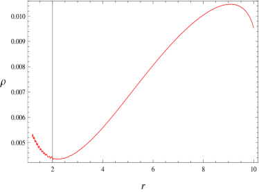
Figure 9: Evolution of $\rho$ and $\rho+p$ for isotropic case.

3.4 Specific EoS $p_{r}=k\rho$

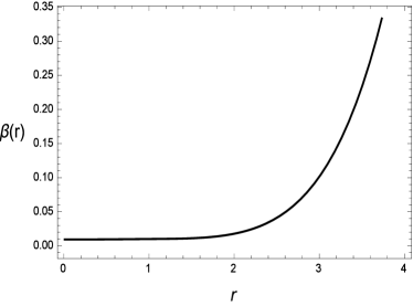
Figure 10: Evolution of $\beta(r)$ and $\beta^{\prime}(r)$ versus $r$. Herein, for the EoS $p_{r}=k\rho$ we set $\lambda=-2,\alpha=0.1,\beta=-30,k=0.001$.

Figure 11: Evolution of $\beta(r)-r$ for EoS $p_{r}=k\rho$.

In this case, we apply an EoS involving energy density and radial pressure, i.e., $p_{r}=k\rho$. Such EoS has been applied in $f(R)$ and $f(T)$ gravities [14, 23, 24] to discuss the wormhole solutions. Using the above defined EoS along with dynamical equation, we find the following constraint to calculate the shape function.

$$\frac{1}{r(1+\lambda)(1+2\lambda)}e^{-b}\bigg{[}4\gamma(23+62\lambda-k(37+58\lambda))+e^{3b}(1+k)\bigg{(}r^{4}(1+2\lambda)$$

$$- 2r^{2}(\alpha+3\alpha\lambda)+4(\gamma+4\gamma\lambda)\bigg{)}-2e^{b}\bigg{(}-30\gamma(-3+5k+8(k-1)\lambda)+r^{2}$$

$$\times \alpha\big{(}-7-15\lambda+k(5+9\lambda)\big{)}\bigg{)}-e^{2b}\bigg{(}-12r^{2}\alpha(k-1)(1+2\lambda)+r^{4}(1+k)$$

$$\times (1+2\lambda)+12\gamma(k(13+22\lambda)-7-18\lambda)\bigg{)}+r\bigg{(}r^{2}\bigg{(}3e^{b}\big{(}r^{2}\alpha-6\gamma\big{)}\bigg{(}k(3\lambda$$

$$+ 2)-\lambda\bigg{)}+2\gamma\bigg{(}20+29\lambda+k\big{(}32+53\lambda)\bigg{)}\bigg{)}b^{\prime 3}+30r^{3}\gamma\bigg{(}\lambda-k(2+3\lambda)\bigg{)}b^{\prime 4}$$

$$+ 6rb^{\prime 2}\bigg{(}2\gamma(11k-3+14(k-1)\lambda)-e^{b}\bigg{(}r^{2}\alpha(1+k)(1+2\lambda)+2\gamma(7k-12$$

$$\times \lambda+8k\lambda-3)\bigg{)}+11r^{2}\gamma\bigg{(}k(2+3\lambda)-\lambda\bigg{)}b^{\prime\prime}\bigg{)}+b^{\prime}\bigg{(}12\big{(}e^{b}-1\big{)}\gamma\bigg{(}8+k\big{(}e^{b}$$

$$- 1\big{)}(\lambda-1)+13\lambda+3e^{b}\lambda\bigg{)}+e^{b}r^{2}\bigg{(}-2\alpha\bigg{(}k(4+3\lambda)-5\lambda\bigg{)}+e^{b}\bigg{(}-6\alpha(1$$ (27)

$$+ k)\lambda+r^{2}(k+2k\lambda)\bigg{)}\bigg{)}+r^{2}\bigg{(}-7e^{b}\big{(}r^{2}\alpha-6\gamma\big{)}\bigg{(}k(2+3\lambda)-\lambda\bigg{)}-6\gamma\big{(}8$$

$$+ 7\lambda+9k(2+3\lambda)\big{)}\bigg{)}b^{\prime\prime}+12r^{3}\gamma(\lambda-k(2+3\lambda))b^{(3)}\bigg{)}+2r\bigg{(}\bigg{(}6\gamma(4+11\lambda$$

$$- 3k(2+3\lambda))+e^{b}\bigg{(}r^{2}\alpha(4+2k+7\lambda+3k\lambda)+6\gamma(6k-4-11\lambda+9k\lambda)\bigg{)}\bigg{)}$$

$$\times b^{\prime\prime}+6r^{2}\gamma\bigg{(}\lambda-k(2+3\lambda)\bigg{)}b^{\prime\prime 2}+r\bigg{(}e^{b}\big{(}r^{2}\alpha-6\gamma\big{)}+6\gamma\bigg{)}\bigg{(}-\lambda+k(2$$

$$+ 3\lambda\bigg{)}b^{(3)}\bigg{)}\bigg{)}\bigg{]}=0,$$

Again we transform the above equation in terms of shape function $\beta(r)$ and employ the numerical approach to show the behavior of flaring out condition and asymptotic flatness. The left plot of Fig. 10 shows $\beta(r)$ as increasing function of $r$. In this case, throat is located at $r=0.0093117$ with $\beta(r_{0})=r_{0}$ and $\beta^{\prime}(r_{0})<1$, the behavior of $\beta^{\prime}(r)$ is shown in right plot of Fig. 10. Moreover, Fig. 11 shows that our solutions satisfy the flaring out condition but this solution does not satisfy the asymptotically flat condition, i.e., $\beta(r)/r\rightarrow 0$ as $r\rightarrow\infty$. The qualitative behavior of $\rho$ and $\rho+p_{t}$ is shown in Fig. 12. Here, we find that the WEC and NEC are not satisfied, so in this case a realistic wormhole is not possible. Hence, the effective curvature contributions in the form of exotic matter help to sustain the wormhole solution.

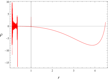
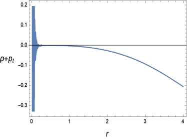
Figure 12: Evolution of $\rho$ and $\rho+p_{t}$.

4 Summary

In GR, wormhole solutions contain a fundamental ingredient, that is, the violation of energy condition in a given space-time. It is taken into consideration that one may impose the principle of modified Einstein field equation by effective stress energy momentum tensor threading the wormholes satisfy the energy conditions and the higher order curvature derivative terms can support geometries of the non-standard wormholes. In this manuscript, we have investigated whether the ordinary matter can support wormholes in $f(R,T)$ modified gravity. For this purpose, we have examined the behavior of energy conditions, i.e., WEC and NEC, for three different fluids: barotropic, isotropic and anisotropic fluids in separate cases.

In literature, it is pointed out that the theoretical advances in the last decades indicate that pressures within highly compact astrophysical objects are anisotropic, i.e., radial pressure $p_{r}$ is not equal to tangential pressure $p_{t}$ in such objects. Anisotropic matter is more general case than isotropic/barotropic case, so it is interesting to examine the existence of wormhole using such matter contents. In this paper, we examined the existence of wormhole solutions using different matter sources. In literature, different techniques have been used to discuss wormhole solutions. One technique is to consider shape function and explore the behavior of energy conditions and the other technique is to calculate shape function by taking some assumption for matter ingredients. In this paper, we are using $f(R,T)$ gravity that involves coupling of matter and Ricci scalar, therefore the resulting equations are quite complicated being highly non-linear with six unknowns namely $\rho,~{}p_{t},~{}p_{r},~{}b,~{}a$ and $f(R)$, therefore we should take some assumptions.

In anisotropic case, it is very difficult to explore the form of shape function from field equations, therefore we explore the behavior of energy condition bounds to check possible existence of wormholes by assuming a viable form of shape function. In other two cases, that is barotropic and isotropic matter sources, the equations are less complicated, therefore we have explored the physical behavior of shape function also. Basically, our purpose is to check whether the coupling of Ricci scalar with matter field can support to existence of wormhole geometries in such theory. In order to discuss wormhole geometries, we have taken some viable conditions. In all cases, we have assumed a well-defined $f(R)$ model defined as $f(R,T)=f_{1}(R)+{\lambda}T$, where $\lambda\in\mathbb{R}$. In anisotropic case, we have discussed the existence of wormhole solutions by taking a particular choice of shape function. Whereas for the other two cases, we have solved the field equation numerically to investigate the behavior of shape function. In case of anisotropic fluid, the behavior of energy constraints have been discussed for two cases of coupling parameter: $\lambda>0$ and $\lambda<-1$. For $\lambda<-1$, it is observed that the WEC is valid for positive values of $\alpha$, while the small validity regions can be found when $\alpha<0$. For $\lambda<-1$, it is observed that the validity regions for WEC can be increased by taking large values of $\alpha$. For $\lambda>0$, the validity of WEC requires negative range of $\alpha$ whereas small validity regions can be found for $\alpha>0$.

Firstly, in our obtained result, wormhole solutions exist but these are not realistic or physically reasonable as one cannot find out the similarity regions for the compatibility of energy bounds, although it is mathematically well-defined problem. Our obtained results are consistent with the works already available in literature [27]. Our results are also similar to that obtained in simple $f(R)$ gravity [14] (that is the case $\lambda=0$). It is interesting to mention here that in their study, both energy bounds, i.e., WEC and DEC are violated in anisotropic and isotropic cases, only in barotropic case, there are some regions where these conditions are compatible while in our case, only DEC energy bound is violated for anisotropic case. In other cases, these conditions remain compatible for some specific ranges of parameters. This difference of result may be arisen due to the presence of curvature-matter coupling term.

In literature, the existence of wormhole solutions in curvature-matter coupled gravity has been discussed by Bertolami and Ferreira [28] and Garcia and Lobo [29]. In both these studies, they have presented a very restricted analysis in this sense that they have used linear functions as $f(R)$ model and also very specific ranges of free parameters have been discussed. They showed that obtained wormhole solutions are well-behaved satisfying DEC when $\lambda$ is positive and increasing. It is interesting to mention here that our results are more comprehensive than these previous works as we have explored the behavior of involved functions and existence of wormhole by taking all possible ranges of the involved parameters (specifically $\lambda$ can take any value). Furthermore, we have used the Starobinsky model that represents $R^{n}$ extension ($n\geq 3$) instead of linear functions. Garcia and Lobo [30] also discussed the wormhole existence in curvature-matter coupling gravity by taking linear $f(R)$ model with positive increasing ansatz for density which is not a physically reasonable choice for density on cosmological ground (as it should be a decreasing function)

We have also investigated the equilibrium picture of found wormhole solutions with anisotropic matter in this gravity. It is seen that the wormhole solutions are stable as the equilibrium condition involving hydrostatic and anisotropic forces is satisfied. In the case of barotropic and isotropic fluids, we have explored the dynamics of shape function by solving equations numerically. From the graphical illustrations of shape function, it is seen that in isotropic case, all the necessary conditions like asymptotically flatness and flaring out constraint are satisfied which indicates that the obtained micro wormhole is realistic and viable. While in case of barotropic fluid, the asymptotic flatness condition is incompatible therefore, a realistic wormhole solution does not exist. It is interesting to to find wormhole solutions without exotic matter by considering some other different $f(R,T)$ models in this gravity.

References

- [1] Perlmutter, S. et al.: Astrophys. J. 483(1997)565; Perlmutter, S. et al.: Nature 391(1998)51; Perlmutter, S. et al.: Astrophys. J. 517(1999)565.
- [2] Nojiri, S. and Odintsov, S.D.: Phys. Rept. 505(2011)59.
- [3] Starobinsky, A.A.: Phys. Lett. B 91(1980)99; Starobinsky, A.A.: JETP Lett. 86(2007)157.
- [4] Ferraro, R. and Fiorini, F.: Phys. Rev. D 75(2007)084031; Zubair, M. Inter. J. Modern Phys. D 25(2016)1650057.
- [5] Carroll, S. et al.: Phys. Rev. D 71(2005)063513; Cognola.G.: Phys. Rev. D 73(2006)084007.
- [6] Agnese, A.G. and La Camera, M.: Phys. Rev. D 51(1995)2011.
- [7] Kofinas, G. and Saridakis, N.E.: Phys. Rev. D 90(2014)084044.
- [8] Harko, T. et al.: Phys. Rev. D 84(2011)024020.
- [9] Houndjo, M.J.S. et al.: Int. J. Mod. Phys. D 21(2012)1250003.
- [10] Houndjo, M.J.S. et al.: Int. J. Mod. Phys. 2(2012)1250024.
- [11] Sharif, M. and Zubair, M.: JCAP 03(2012)028; Singh, C.P. and Singh, V.: Gen. Relativ. Gravitt. 46(2014)1696; Mubasher et al.: Eur. Phys. J. C 72(2012)1999; Sharif, M. and Zubair, M.: J. Phys. Soc. Jpn. 82(2013)064001; Shabani, H. and Farhoudi, M.: Phys. Rev. D 88(2013)044048; ibid. Phys. Rev. D 90(2014)044031; Santos, A.F.: Modern Phys. Lett. A 28(2013)1350141; M. Sharif, M. Zubair, Gen. Relativ. Gravit. 46(2014)1723; Zubair, M. and Noureen, I.: Eur. Phys. J. C 75(2015)265; Noureen, I. and Zubair, M.: Eur. Phys. J. C 75(2015)62; Noureen, I. and Zubair, M., Bhatti, A.A. and Abbas, G.: Eur. Phys. J. C 75(2015)323; Alvarenga et al.: Phys. Rev. D 87(2013)103526; Baffou et al. Astrophys. Space Sci. 356(2015)173; Shamir, M.F.: Eur. Phys. J. C 75(2015)354; Moraes, P.H.R.S.: Eur. Phys. J. C 75(2015)168; Zubair, M. et al.: Astrophys Space Sci. 361(2016)8; Zubair, M. and Syed M. Ali Hassan.: Astrophys Space Sci. 361(2016)149; Shahbani, H.: arXiv:1604.04616v1.
- [12] Einstein, A. and Rosen, N.: Phys. Rev. 48(1935)73.
- [13] Lobo, F.S.N. and Oliveira, M.A.: Phys. Rev. D 80(2009)104012.
- [14] Sharif, M. and Zahra, Z.: Astrophys. Space Sci. 348(2013)275.
- [15] Morris, M.S. and Thorne, K.S.: Am. J. Phys. 56(1988)395; Morris, M.S., Throne, K.S. and Yurtseve, U.: Phys. Rev. Lett. 61(1988)1446.
- [16] Azizi, T.: Int. J. Theor. Phys. 52(2013)3486.
- [17] Landau, L.D. and Lifshitz, E.M.: The Classical Theory of Fields (Butterworth-Heinemann, 2002).
- [18] Alvarenga et al.: J. Modern Phys. 4(2013)130; Sharif, M. and Zubair, M.: J. Phys. Soc. Jpn. 82 (2013)014002.
- [19] Ozkan, M. and Pang, Y.: Class. Quantum Grav. 31, 205004 (2014).
- [20] Goswami, U.D. and Deka, K.: Int. J. Mod. Phys. D 22(2013)1350083.
- [21] Frolov, A.V.: Phys. Rev. Lett. 101(2008)061103.
- [22] Hu, W. and Sawicki, I.: Phys. Rev. D 76(2007)064004.
- [23] Jamil, M., Momeni, D. and Myrzakulov, R.: Eur. Phys. J. C 73(2013)2267.
- [24] Boehmer, C.G., Harko, T.and Lobo, F.S.N.: Phys. Rev. D 85(2012)044033.
- [25] Pavlovic, P. and Sossich, M.: Eur. Phys. J. C 75(2015)117.
- [26] Dent, J.B. , Dutta, S. and Saridakis, E.N.: J. Cosmol. Astropart. Phys. 009(2011)1101; Sotiriou, T.P., Li, B. and Barrow, J.D.: Phys. Rev. D 83(2011)104030; Li, B., Sotiriou, T.P. and Barrow, J.D.: Phys. Rev. D 83(2011)104017; Zhang, Y., Li, H., Gong, Y. and Zhu, Z.H.: J. Cosmol. Astropart. Phys. 015(2011)1107; Bhattacharya, S. and Chakraborty, S.: arXiv:1506.03968v2.
- [27] Mehdizadeh, M.R., Zangeneh, M.K. and Lobo, F.S.N.: Phys. Rev. D 91(2015)084004; Jamil, M., Momeni, D. and Myrzakulov, R.: Eur. Phys. J. C 73(2013)2267;
- [28] Bertolami, O. and Ferreira, R.Z.: Phys. Rev. D 85(2012)104050.
- [29] Garcia, N.M. and Lobo, F.S.N.: Phys. Rev. D 82(2010)104018.
- [30] Garcia, N.M. and Lobo, F.S.N.: Class. Quantum Grav. 28(2011)085018.