On the Identification and Mitigation of Weaknesses in the Knowledge Gradient Policy for Multi-Armed Bandits

James Edwards
STOR-i Centre for Doctoral Training, Lancaster University, Lancaster,LA1 4YF, UK j.edwards4@lancaster.ac.uk
Paul Fearnhead
Department of Mathematics and Statistics, Lancaster University, Lancaster, LA1 4YF, UK p.fearnhead@lancaster.ac.uk
Kevin Glazebrook
Department of Management Science, Lancaster University, LA1 4YX, UK k.glazebrook@lancaster.ac.uk

The Knowledge Gradient (KG) policy was originally proposed for offline ranking and selection problems but has recently been adapted for use in online decision-making in general and multi-armed bandit problems (MABs) in particular. We study its use in a class of exponential family MABs and identify weaknesses, including a propensity to take actions which are dominated with respect to both exploitation and exploration. We propose variants of KG which avoid such errors. These new policies include an index heuristic which deploys a KG approach to develop an approximation to the Gittins index. A numerical study shows this policy to perform well over a range of MABs including those for which index policies are not optimal. While KG does not take dominated actions when bandits are Gaussian, it fails to be index consistent and appears not to enjoy a performance advantage over competitor policies when arms are correlated to compensate for its greater computational demands.

1 Introduction

Bayes sequential decision problems (BSDPs) constitute a large class of optimisation problems in which decisions (i) are made in time sequence and (ii) impact the system of interest in ways which may be not known or only partially known. Moreover, it is possible to learn about unknown system features by taking actions and observing outcomes. This learning is modelled using a Bayesian framework. One important subdivision of BSDPs is between offline and online problems. In offline problems some decision is required at the end of a time horizon and the purpose of actions through the horizon is to accumulate information to support effective decision-making at its end. In online problems each action can bring an immediate payoff in addition to yielding information which may be useful for subsequent decisions. This paper is concerned with a particular class of online problems although it should be noted that some of the solution methods have their origins in offline contexts.

The sequential nature of the problems coupled with imperfect system knowledge means that decisions cannot be evaluated alone. Effective decision-making needs to account for possible future actions and associated outcomes. While standard solution methods such as stochastic dynamic programming can in principle be used, in practice they are computationally impractical and heuristic approaches are generally required. One such approach is the knowledge gradient (KG) heuristic. Gupta and Miescke, [8] originated KG for application to offline ranking and selection problems. After a period of time in which it appears to have been studied little, Frazier et al., [5] expanded on KG’s theoretical properties. It was adapted for use in online decision-making by Ryzhov et al., [14] who tested it on multi-armed bandits (MABs) with Gaussian rewards. They found that it performed well against an index policy which utilised an analytical approximation to the Gittins index; see Gittins et al., [7]. Ryzhov et al., [12] have investigated the use of KG to solve MABs with exponentially distributed rewards while Powell and Ryzhov, [10] give versions for Bernoulli, Poisson and uniform rewards, though without testing performance. They propose the method as an approach to online learning problems quite generally, with particular emphasis on its ability to handle correlated arms. Initial empirical results were promising but only encompassed a limited range of models. This paper utilises an important sub-class of MABs to explore properties of the KG heuristic for online use. Our investigation reveals weaknesses in the KG approach. We inter alia propose modifications to mitigate these weaknesses.

In Section 2 we describe a class of exponential family MABs that we will focus on, together with the KG policy for them. Our main analytical results revealing weaknesses in KG are given in Section 3. Methods aimed at correcting these KG errors are discussed in Section 4 and are evaluated in a computational study which is reported in Section 5. In this study a range of proposals are assessed for Bernoulli and Exponential versions of our MAB models. Gaussian MABs have characteristics which give the operation of KG distinctive features. The issues for such models are discussed in Section 6, together with an associated computational study in Section 6.1. Section 7 identifies some key conclusions to be drawn.

2 A class of exponential family multi-armed bandits

2.1 Multi-Armed Bandit Problems for Exponential Families

We consider multi-armed bandits (MABs) with geometric discounting operating over a time horizon $T\in\mathbb{Z}^{+}\cup\{\infty\}$ which may be finite or not. Rewards are drawn from exponential families with independent conjugate priors for the unknown parameters. More specifically the set up is as follows:

1. At each decision time $t\in\{0,1,\ldots,T-1\}$ an action $a\in\{1,\ldots,k\}$ is taken. Associated with each action, $a$, is an (unknown) parameter, which we denote as $\theta_{a}$. Action $a$ (pulling arm $a$) yields a reward which is drawn from the density (relative to some $\sigma$-finite measure on $\mathbb{R}$)

   $$f(y\mid\theta_{a})=e^{\theta_{a}y-\psi(\theta_{a})},y\in\Omega,\theta_{a}\in\Theta,$$ (2.1)

   where $\Omega\subseteq\mathbb{R}$ is the support of $f,$ $\psi$ is a cumulant generating function and parameter space $\Theta\subseteq\mathbb{R}$ is such that $\psi\left(\theta\right)<\infty,\;\forall\theta\in\Theta$. Reward distributions are either discrete or absolutely continuous, with $\Omega$ a discrete or continuous interval $\left[\min\Omega,\max\Omega\right]$ where $-\infty\leq\min\Omega<\max\Omega\leq\infty$. We shall take a Bayesian approach to learning about the parameters $\theta_{a}$.

2. We assume independent conjugate priors for the unknown $\theta_{a}$ with Lebesgue densities given by

   $$g(\theta_{a}\mid\Sigma_{a},n_{a})\propto e^{\Sigma_{a}\theta_{a}-n_{a}\psi(\theta_{a})},\theta_{a}\in\Theta,1\leq a\leq k,$$ (2.2)

   where $\Sigma_{a}$ and $n_{a}$ are known hyper-parameters. This then defines a predictive density

   $$p(y\mid\Sigma_{a},n_{a})=\int_{\Theta}f(y\mid\theta_{a})g(\theta_{a}\mid\Sigma_{a},n_{a})d\theta_{a}$$ (2.3)

   which has mean $\frac{\Sigma_{a}}{n_{a}}$. Bayesian updating following an observed reward $y$ on arm $a$ produces a posterior $p(\theta_{a}|y)=g(\theta_{a}|\Sigma_{a}+y,n_{a}+1)$. Thus at each time we can define an arm’s informational state as the current value of hyper-parameters $\Sigma_{a},n_{a}$, such that the posterior for $\theta_{a}$ given the observations to date is $g(\theta_{a}|\Sigma_{a},n_{a})$. The posterior for each arm is independent so the informational states of arms not pulled at $t$ are unchanged.

3. The total return when reward $y_{t}$ is received at time $t$ is given by $\sum\nolimits_{t=0}^{T-1}\gamma^{t}y_{t},$ where discount rate $\gamma$ satisfies either $0<\gamma\leq 1$ when $T<\infty$ or $0<\gamma<1$ when $T=\infty$. The objective is to design a policy, a rule for choosing actions, to maximise the Bayes’ return, namely the total return averaged over both realisations of the system and prior information.

The current informational state for all arms, denoted $(\mathbf{\Sigma},\mathbf{n)}=\left\{(\Sigma_{a},n_{a}),1\leq a\leq k\right\}$ summarises all the information in the observations up to the current time.

When $0<\gamma<1,T=\infty$ the Bayes’ return is maximised by the Gittins Index (GI) policy, see Gittins et al., [7]. This operates by choosing, in the current state, any action $a$, satisfying

$$\nu^{GI}(\Sigma_{a},n_{a},\gamma)=\max_{1\leq b\leq k}\nu^{GI}(\Sigma_{b},n_{b},\gamma)\,,$$ (2.4)

where $\nu^{GI}$ is the Gittins index. We describe Gittins indices in Section 4 along with versions adapted for use in problems with $0<\gamma\leq 1,T<\infty$. Given the challenge of computing Gittins indices and the general intractability of deploying dynamic programming to solve online problems, the prime interest is in the development of heuristic policies which are easy to compute and which come close to being return maximising.

2.2 The Knowledge Gradient Heuristic

The Knowledge Gradient policy KG is a heuristic which bases action choices both on immediate returns $\frac{\Sigma_{a}}{n_{a}}$ and also on the changes in informational state which flow from a single observed reward. It is generally fast to compute. To understand how KG works for MABs suppose that the decision time is $t$ and that the system is in information state $(\mathbf{\Sigma,n})$ then. The current decision is taken to be the last opportunity to learn and so from time $t+1$ through to the end of the horizon whichever arm has the highest mean reward following the observed reward at $t$ will be pulled at all subsequent times. With this informational constraint, the best arm to pull at $t$ (and the action mandated by KG in state $\left(\mathbf{\Sigma,n}\right)$) is given by

$$A^{KG}(\mathbf{\Sigma,n,}t)=\arg\max_{a}\left\{\frac{\Sigma_{a}}{n_{a}}+H(\gamma,s)\max_{1\leq b\leq k}E\left(\frac{\Sigma_{b}+I_{a}Y}{n_{b}+I_{a}}\mid\mathbf{\Sigma,n,}a\right)\right\},$$ (2.5)

where $Y$ is the observed reward at $t$ and $I_{a}$ is an indicator taking the value $1$ if action $a$ is taken at $t,$ $0$ otherwise. The conditioning indicates that the reward $Y$ depends upon the current state $\left(\mathbf{\Sigma,n}\right)$ and the choice of action $a$. The constant $H(\gamma,s)$ is a suitable multiplier of the mean return of the best arm at $t+1$ to achieve an accumulation of rewards for the remainder of the horizon (denoted here by $s=T-t$). It is given by

$$H(\gamma,s)=\begin{cases}\frac{\gamma(1-\gamma^{s-1})}{1-\gamma}&\mbox{if }0<\gamma<1,T<\infty\\ \frac{\gamma}{1-\gamma}&\mbox{if }0<\gamma<1,T=\infty\\ s-1&\mbox{if }\gamma=1,T<\infty.\end{cases}$$ (2.6)

KG can be characterised as the policy resulting from the application of a single policy improvement step to a policy which always pulls an arm with the highest prior mean return throughout. Note that for $\left(\gamma,T\right)\in(0,1)\times\mathbb{Z}^{+},$ $H(\gamma,s)$ is increasing in both $\gamma$ ($T$ fixed) and in $T$ ($\gamma$ fixed). For any sequence of $\left(\gamma,T\right)$ values approaching the limit $\left(1,\infty\right)$ in a manner which is co-ordinatewise increasing, the value of $H(\gamma,s)$ diverges to infinity. This fact is utilised heavily in Section 3.

We now develop an equivalent characterisation of KG based on Ryzhov et al., [14] which will be more convenient for what follows. We firstly develop an expression for the change in the maximal mean reward available from any arm when action $a$ is taken in state $\left(\mathbf{\Sigma,n}\right)$. We write

$$\nu_{a}^{KG}\left(\mathbf{\Sigma,n}\right)=E\left\{\max_{1\leq b\leq k}\mu_{b}^{+1}-\max_{1\leq b\leq k}\mu_{b}\mid\mathbf{\Sigma,n,}a\right\},$$ (2.7)

where $\mu_{b}$ is the current arm $b$ mean return $\frac{\Sigma_{b}}{n_{b}}$ and $\mu_{b}^{+1}$ is the mean return available from arm $b$ at the next time conditional on the observed reward resulting from action $a$. Please note that $\mu_{b}^{+1}$ is a random variable. It is straightforward to show that

$$A^{KG}(\mathbf{\Sigma,n,}t)=\arg\max_{1\leq a\leq k}\left\{\mu_{a}+H(\gamma,s)\nu_{a}^{KG}(\mathbf{\Sigma,n})\right\}.$$ (2.8)

Hence KG gives a score to each arm and chooses the arm of highest score. It is not an index policy because the score depends upon the informational state of arms other than the one being scored. That said, there are similarities between KG scores and Gittins indices. The Gittins index $\nu^{GI}(\Sigma_{a},n_{a})$ exceeds the mean return $\frac{\Sigma_{a}}{n_{a}}$ by an amount termed the uncertainty or learning bonus. This bonus can be seen as a measure of the value of exploration in choosing arm $a$. The quantity $H(\gamma,s)\nu_{a}^{KG}\left(\mathbf{\Sigma,n}\right)$ in the KG score is an alternative estimate of the learning bonus. Assessing the accuracy of this estimate will give an indication of the strengths and weaknesses of the policy.

2.3 Dominated arms

In our discussion of the deficiencies of the KG policy in the next section we shall focus, among other things, on its propensity to pull arms which are suboptimal to another arm with respect to both exploitation and exploration. Hence there is an alternative which is better both from an immediate return and from an informational perspective. We shall call such arms dominated. We begin our discussion with a result concerning properties of Gittins indices established by Yu, [19].

Theorem 1

The Gittins index $\nu^{GI}\left(c\Sigma,cn,\gamma\right)$ is decreasing in $c\in\mathbb{R}^{+}$ for any fixed $\Sigma,n,\gamma$ and is increasing in $\Sigma$ for any fixed $c,n,\gamma$.

We proceed to a simple corollary whose proof is omitted. The statement of the result requires the following definition.

Definition 2

An arm in state $\left(\Sigma,n\right)$ dominates one in state $\left(\Sigma^{\prime},n^{\prime}\right)$ if and only if $\frac{\Sigma}{n}>\frac{\Sigma^{\prime}}{n^{\prime}}$ and $n<n^{\prime}$.

Corollary 3

The GI policy never chooses dominated arms.

Hence pulling dominated arms can never be optimal for infinite horizon MABs. We shall refer to the pulling of a dominated arm as a dominated action in what follows. Exploration of the conditions under which KG chooses dominated actions is a route to an understanding of its deficiencies and prepares us to propose modifications to it which achieve improved performance. This is the subject matter of the following two sections.

3 The KG policy and dominated actions

3.1 Conditions for the choice of dominated actions under KG

This section will elucidate sufficient conditions for the KG policy to choose dominated arms. A key issue here is that the quantity $\nu_{a}^{KG}$ (and hence the KG learning bonus) can equal zero in cases where the true learning bonus related to a pull of arm $a$ may be far from zero. Ryzhov et al., [14] stated that $\nu_{a}^{KG}>0$. However, crucially, that paper only considered Gaussian bandits. The next lemma is fundamental to the succeeding arguments. It says that, for sufficiently high $\gamma$, the KG policy will choose the arm with the largest $\nu^{KG}$.

Lemma 4

$\forall\mathbf{\Sigma},\mathbf{n},t$ for which $max_{a}\nu_{a}^{KG}\left(\mathbf{\Sigma},\mathbf{n}\right)>0$ $\exists\gamma^{\ast},T^{\ast}$ such that $\gamma>\gamma^{\ast},T>T^{\ast}\Rightarrow A^{KG}\left(\mathbf{\Sigma},\mathbf{n},t\right)=\arg\max_{a}\nu_{a}^{KG}\left(\mathbf{\Sigma},\mathbf{n}\right)$.

• Proof. The result is a trivial consequence of the definition of the KG policy in Section 2.2 together with the fact that $H(\gamma,s)$ diverges to infinity in the manner described in Section 2.  

The next result gives conditions under which $\nu_{a}^{KG}\left(\mathbf{\Sigma},\mathbf{n}\right)=0$.

Lemma 5

Let $C_{a}\left(\mathbf{\Sigma},\mathbf{n}\right)$ denote $\max_{b\neq a}\mu_{b}=\max_{b\neq a}\frac{\Sigma_{b}}{n_{b}}$. If $a\in\arg\max_{b}\mu_{b}$ and the observation state space, $\Omega$, is bounded below with minimum value $\min\Omega$ then

$$\nu_{a}^{KG}\left(\mathbf{\Sigma},\mathbf{n}\right)=0\Leftrightarrow\frac{\Sigma_{a}+\min\Omega}{n_{a}+1}\geq C_{a}\left(\mathbf{\Sigma},\mathbf{n}\right);$$ (3.1)

while if $a\notin\arg\max_{b}\mu_{b}$ and $\Omega$ is bounded above with maximum value $\max\Omega$ then

$$\nu_{a}^{KG}\left(\mathbf{\Sigma},\mathbf{n}\right)=0\Leftrightarrow\frac{\Sigma_{a}+\max\Omega}{n_{a}+1}\leq C_{a}\left(\mathbf{\Sigma},\mathbf{n}\right).$$ (3.2)

In cases where $a\in\arg\max_{b}\mu_{b}$ with $\Omega$ unbounded below, and where $a\notin\arg\max_{b}\mu_{b}$ with $\Omega$ is unbounded above, we have $\nu_{a}^{KG}\left(\mathbf{\Sigma},\mathbf{n}\right)>0$.

• Proof. Note that

  $$\nu_{a}^{KG}\left(\mathbf{\Sigma},\mathbf{n}\right) =E_{Y_{a}}\left[\max_{b}\mu_{b}^{+1}-\max_{b}\mu_{b}\mid\mathbf{\Sigma},\mathbf{n,}a\right]$$

  $$=E_{Y_{a}}\left[\max\left(\mu_{a}^{+1},C_{a}\left(\mathbf{\Sigma},\mathbf{n}\right)\right)\mid\mathbf{\Sigma},\mathbf{n,}a\right]-\max_{b}\mu_{b}.$$ (3.3)

  Hence

  $$\nu_{a}^{KG}\left(\mathbf{\Sigma},\mathbf{n}\right)=0\Leftrightarrow E_{Y_{a}}\left[\max\left(\mu_{a}^{+1},C_{a}\left(\mathbf{\Sigma},\mathbf{n}\right)\right)\mid\mathbf{\Sigma},\mathbf{n,}a\right]=\max_{b}\mu_{b}.$$ (3.4)

  If $a\in\arg\max_{b}\mu_{b}$ and so $max_{b}\mu_{b}=\mu_{a}$ then, observing that

  $$E_{Y_{a}}\left[\max\left(\mu_{a}^{+1},C_{a}\left(\mathbf{\Sigma},\mathbf{n}\right)\right)\mid\mathbf{\Sigma},\mathbf{n,}a\right]\geq E_{Y_{a}}\left[\mu_{a}^{+1}\mid\mathbf{\Sigma},\mathbf{n,}a\right]=\mu_{a},$$ (3.5)

  we infer from equation Eq. (3.4) that $\nu_{a}^{KG}\left(\mathbf{\Sigma},\mathbf{n}\right)=0$ if and only if

  $$\max\left(\mu_{a}^{+1},C_{a}\left(\mathbf{\Sigma},\mathbf{n}\right)\right)=\mu_{a}^{+1}\Leftrightarrow\mu_{a}^{+1}\geq C_{a}\left(\mathbf{\Sigma},\mathbf{n}\right)$$ (3.6)

  with probability $1$ under the distribution of $Y_{a}$. Under our set up as described in Section 2, this condition is equivalent to the right hand side of Eq. (3.1). If $a\notin\arg\max_{b}\mu_{b}$ then $max_{b}\mu_{b}=C_{a}\left(\mathbf{\Sigma},\mathbf{n}\right)$ and so, suitably modifying the previous argument, we infer that $\nu_{a}^{KG}\left(\mathbf{\Sigma},\mathbf{n}\right)=0$ if and only if

  $$\max\left(\mu_{a}^{+1},C_{a}\left(\mathbf{\Sigma},\mathbf{n}\right)\right)=C_{a}\left(\mathbf{\Sigma},\mathbf{n}\right)\Leftrightarrow\mu_{a}^{+1}\leq C_{a}\left(\mathbf{\Sigma},\mathbf{n}\right)$$ (3.7)

  with probability $1$ under the distribution of $Y_{a}$. Under our set up as described in Section 2, this condition is equivalent to the right hand side of Eq. (3.2). The unbounded cases follow directly from the formula for $\nu_{a}^{KG}(\mathbf{\Sigma},\mathbf{n})$ as the change in $\mu_{a}$ due to an observation has no finite limit in the direction(s) of unboundedness. This completes the proof.  

Informally, $\nu_{a}^{KG}=0$ if no outcome from a pull on arm $a$ will change which arm has maximal mean value. When $a\in\arg\max_{b}\mu_{b}$ this depends on the lower tail of the distribution of $Y_{a}$ while if $a\notin\arg\max_{b}\mu_{b}$ it depends on the upper tail. This asymmetry is important in what follows.

Theorem 6

If $\Omega$ is bounded below then there are choices of $\mathbf{\Sigma,n,}\gamma,T$ for which the KG policy chooses dominated arms.

• Proof. If we consider cases for which

  $$\frac{\Sigma_{1}}{n_{1}}>\frac{\Sigma_{2}}{n_{2}},n_{1}<n_{2};\Sigma_{b}=c\Sigma_{2},n_{b}=cn_{2},3\leq b\leq k,c\geq 1$$ (3.8)

  then it follows that $\mu_{2}=\mu_{b},\nu_{2}^{KG}\geq\nu_{b}^{KG},3\leq b\leq k$, and all arms except $1$ and $2$ can be ignored in the discussion. We first suppose that $\Omega$ unbounded above. It follows from Lemma 5 that $\nu_{2}^{KG}(\mathbf{\Sigma},\mathbf{n})>0$. Since $\min\Omega>-\infty,$ we can further choose $(\mathbf{\Sigma},\mathbf{n})$ such that

  $$\frac{\Sigma_{1}+\min\Omega}{n_{1}+1}\geq\frac{\Sigma_{2}}{n_{2}}=C_{1}(\mathbf{\Sigma},\mathbf{n}).$$ (3.9)

  From the above result we infer that $\nu_{1}^{KG}(\mathbf{\Sigma},\mathbf{n})=0$. We now suppose that $\Omega$ is bounded above, and hence that $\infty>\max\Omega>\min\Omega>-\infty$. Choose $(\mathbf{\Sigma},\mathbf{n})$ as follows: $\Sigma_{1}=\max\Omega+2\min\Omega,n_{1}=3,\Sigma_{2}=\max\Omega+3\min\Omega,n_{2}=4$. It is trivial that these choices mean that arm $1$ dominates arm $2$. We have that

  $$\frac{\Sigma_{1}+\min\Omega}{n_{1}+1}=\frac{\max\Omega+3\min\Omega}{4}=\frac{\Sigma_{2}}{n_{2}}=C_{1}(\mathbf{\Sigma},\mathbf{n})$$ (3.10)

  and hence that $\nu_{1}^{KG}(\mathbf{\Sigma},\mathbf{n})=0$. Further we have that

  $$\frac{\Sigma_{2}+\max\Omega}{n_{2}+1}=\frac{2\max\Omega+3\min\Omega}{5}>\frac{\Sigma_{1}}{n_{1}}=C_{2}(\mathbf{\Sigma},\mathbf{n})$$ (3.11)

  and hence that $\nu_{2}^{KG}(\mathbf{\Sigma},\mathbf{n})>0$. In both cases discussed (ie, $\Omega$ bounded and unbounded above) we conclude from Lemma 4 the existence of $t,\gamma^{\ast},T^{\ast}$ such that $\gamma>\gamma^{\ast},T>T^{\ast}\Rightarrow A^{KG}(\mathbf{\Sigma},\mathbf{n},t)=\arg\max_{a}\nu_{a}^{KG}(\mathbf{\Sigma},\mathbf{n})=2,$ which is a dominated arm, as required. This concludes the proof.  

Although the part of the above proof dealing with the case in which $\Omega$ is bounded above identifies a specific state in which KG will choose a dominated arm when $H(\gamma,s)$ is large enough, it indicates how such cases may be identified more generally. These occur when the maximum positive change in the mean of the dominated arm ($\mu_{2}\rightarrow\mu_{2}^{+1}$) is larger than the maximum negative change in the mean of the dominating arm ($\mu_{1}\rightarrow\mu_{1}^{+1}$). This can occur both when the $Y_{a}$ have distributions skewed to the right and also where the corresponding means are both small, meaning that a large $y$ can effect a greater positive change in $\mu_{2}$ than can a small $y$ a negative change in $\mu_{1}$. A detailed example of this is given for the Bernoulli MAB in the next section. Similar reasoning suggests that the more general sufficient condition for KG to choose dominated arms, namely $\nu_{2}^{KG}\left(\mathbf{\Sigma},\mathbf{n}\right)>\nu_{1}^{KG}\left(\mathbf{\Sigma},\mathbf{n}\right)$ with arm $2$ dominated, will hold in cases with $\Omega$ unbounded above if the distribution of $Y_{a}$ has an upper tail considerably heavier than its lower tail.

3.2 Stay-on-the winner rules

Berry and Fristedt, [1] demonstrated that optimal policies for MABs with Bernoulli rewards and general discount sequences (including all cases considered here) have a stay-on-the-winner property. If arm $a$ is optimal at some epoch and a pull of $a$ yields a success ($y_{a}=1$) then arm $a$ continues to be optimal at the next epoch. Yu, [19] extends this result to the exponential family considered here in the following way: an optimal arm continues to be optimal following an observed reward which is sufficiently large. The next result is an immediate consequence.

Lemma 7

Suppose that $\Omega$ is bounded above. If arm $a$ is optimal at some epoch and a pull of $a$ yields a maximal reward ($y_{a}=\max\Omega$) then arm $a$ is optimal at the next epoch.

The following result states that the KG policy does not share the stay-on-the-winner character of optimal policies as described in the preceding lemma. In its statement we use $\mathbf{e}_{a}$ for the $k-$vector whose $ath$ component is $1,$ with zeroes elsewhere.

Proposition 8

If $\Omega$ is bounded above and below $\exists$ choices of $\mathbf{\Sigma,n,}t,\gamma,T$ and $a$ for which $A^{KG}\left(\mathbf{\Sigma},\mathbf{n},t\right)=a$, $A^{KG}\left(\mathbf{\Sigma+\max\Omega e}_{a},\mathbf{n+e}_{a},t\right)\neq a$.

• Proof. For the reasons outlined in the proof of Theorem 6 we may assume without loss of generality that $k=2$. As in that proof we consider the state $\left(\mathbf{\Sigma,n}\right)$ with $\Sigma_{1}=\max\Omega+2\min\Omega,n_{1}=3,\Sigma_{2}=\max\Omega+3\min\Omega,n_{2}=4$. We suppose that a pull of arm $2$ yields an observed reward equal to $\max\Omega$. This takes the process state to $\left(\mathbf{\Sigma+\max\Omega e}_{2},\mathbf{n+e}_{2},t\right)=\left(\mathbf{\Sigma}^{/},\mathbf{n}^{/}\right),$ say. We use the dashed notation for quantities associated with this new state. Observe that $\mu_{2}^{/}>\mu_{1}^{/}$ and hence that $2\in\arg\max_{b}\mu_{b}^{/}$. We note that

  $$\frac{\Sigma_{2}^{/}+\min\Omega}{n_{2}^{/}+1}=\frac{2\max\Omega+4\min\Omega}{\text{ }6}=\mu_{1}^{/}=C_{2}\left(\mathbf{\Sigma}^{/},\mathbf{n}^{/}\right),$$ (3.12)

  which implies via Lemma 5 that $\nu_{2}^{KG}\left(\mathbf{\Sigma}^{/},\mathbf{n}^{/}\right)=0$. We also have that

  $$\frac{\Sigma_{1}^{/}+\max\Omega}{n_{1}^{/}+1}=\frac{2\max\Omega+2\min\Omega}{4}>\mu_{2}^{/}=C_{1}\left(\mathbf{\Sigma}^{/},\mathbf{n}^{/}\right),$$ (3.13)

  which implies via Lemma 5 that $\nu_{1}^{KG}\left(\mathbf{\Sigma}^{/},\mathbf{n}^{/}\right)>0$. The existence of $t,$ $\gamma,T$ for which $A^{KG}\left(\mathbf{\Sigma},\mathbf{n},t\right)=2$ while $A^{KG}\left(\mathbf{\Sigma}^{/},\mathbf{n}^{/},t+1\right)=A^{KG}\left(\mathbf{\Sigma+\max\Omega e}_{2},\mathbf{n+e}_{2},t\right)\neq 2$ now follows from Lemma 4.  

3.3 Examples

We will now give more details of how the KG policy chooses dominated actions in the context of two important members of the exponential family.

3.3.1 Exponential rewards

Suppose that $Y_{a}\mid\theta_{a}\backsim Exp(\theta_{a})$ and $\theta_{a}\backsim Gamma(n_{a}+1,\Sigma_{a})$ which yields the unconditional density for $Y_{a}$ given by

$$g_{a}(y)=(n_{a}+1)\Sigma_{a}^{n_{a}+1}(\Sigma_{a}+1)^{-n_{a}-2},y\geq 0,$$ (3.14)

with $E(Y_{a})=\frac{\Sigma_{a}}{n_{a}}$. Let arm $1$ dominate arm $2$. For this case $\Omega=[0,\infty)$ and from Lemma 5, the unboundedness of $\Omega$ above means that $\nu_{2}^{KG}(\mathbf{\Sigma,n})>0$ while $\nu_{1}^{KG}(\mathbf{\Sigma,n})=0$ if and only if

$$\frac{\Sigma_{1}}{n_{1}+1}\geq\frac{\Sigma_{2}}{n_{2}}.$$ (3.15)

Hence from Lemma 4 we can assert the existence of $t,\gamma,T$ for which KG chooses dominated arm $2$ whenever (Eq. (3.15) holds.

Ryzhov and Powell, [13] discuss the online KG policy for Exponential rewards in detail. They observe that $\nu_{a}^{KG}$ can be zero but do not appear to recognise that this can yield dominated actions under the policy. Later work, [4], showed that this can lead to the offline KG policy never choosing the greedy arm, an extreme case of dominated errors. However, with the online KG policy the greedy arm will eventually be selected as $\nu_{a}^{KG}$ for the other arm tends to zero. These papers note that, in states for which

$$\frac{\Sigma_{1}}{n_{1}+1}\leq\frac{\Sigma_{2}}{n_{2}}\leq\frac{\Sigma_{1}}{n_{1}},$$ (3.16)

the value of $\nu_{1}^{KG}\left(\mathbf{\Sigma},\mathbf{n}\right),$ while not zero, penalises the choice of the greedy arm relative to other arms in a similar way to the bias which yields dominated actions. Policies which mitigate such bias are given in the next section and are evaluated in the computational study following.

3.3.2 Bernoulli rewards

Suppose that $Y_{a}\mid\theta_{a}\backsim Bern\left(\theta_{a}\right),$ with $\theta_{a}\backsim Beta\left(\Sigma_{a},n_{a}-\Sigma_{a}\right)$ and so $\Omega=\left\{0,1\right\}$ and $P\left(Y_{a}=1\right)=\frac{\Sigma_{a}}{n_{a}}=1-P\left(Y_{a}=0\right)$. Since $\Omega$ is bounded above and below, dominated actions under KG will certainly occur. Demonstrating this in terms of the asymmetric updating of Beta priors can be helpful in understanding the more general case of bounded rewards. Use $\delta_{a}^{+}$ and $\delta_{a}^{-}$ for the magnitudes of the upward and downward change in $E\left(Y_{a}\right)$ under success and failure respectively. We have

$$\delta_{a}^{+}=\frac{n_{a}-\Sigma_{a}}{n_{a}\left(n_{a}+1\right)}\;;\;\delta_{a}^{-}=\frac{\Sigma_{a}}{n_{a}\left(n_{a}+1\right)},$$ (3.17)

from which we conclude that $\delta_{a}^{+}\geq\delta_{a}^{-}\Leftrightarrow\mu_{a}\leq 0.5$. Prompted by this analysis, consider a case in which $k=2,\Sigma_{1}=\Sigma_{2};n_{1}+m=n_{2}$ for some $m\in\mathbb{N}^{+}$. Arm $1$ dominates arm $2$. Further, the fact that

$$\frac{\Sigma_{1}+\min\Omega}{n_{1}+1}=\frac{\Sigma_{1}}{n_{1}+1}\geq\frac{\Sigma_{1}}{n_{1}+m}=\frac{\Sigma_{2}}{n_{2}}=C_{1}\left(\mathbf{\Sigma},\mathbf{n}\right)$$ (3.18)

implies via Lemma 5 that $\nu_{1}^{KG}\left(\mathbf{\Sigma},\mathbf{n}\right)=0$. From Lemma 5 we also conclude that

$$\nu_{2}^{KG}\left(\mathbf{\Sigma},\mathbf{n}\right)>0\iff\frac{\Sigma_{2}+\max\Omega}{n_{2}+1}=\frac{\Sigma_{1}+1}{n_{1}+m+1}>\frac{\Sigma_{1}}{n_{1}}=C_{2}\left(\mathbf{\Sigma},\mathbf{n}\right).$$ (3.19)

The strict inequality in the right hand side of Eq. (3.19) will hold whenever $n_{1}>\left(m+1\right)\Sigma_{1}$. Thus, for suitably chosen $t,\gamma$ and $T,$ the KG policy will take dominated actions in a wide range of states. Suppose now that $T=\infty$ and hence the immediate claim is that under the condition $n_{1}>\left(m+1\right)\Sigma_{1}$ the KG policy will take dominated action $2$ for $\gamma$ large enough. We now observe that in practice dominated actions can be taken for quite modest $\gamma$. Returning to the characterisation of the KG policy we infer that in the above example, dominated action $2$ will be chosen whenever

$$n_{1}>\left(m+1\right)\Sigma_{1},\frac{\gamma}{1-\gamma}>\frac{m\left(n_{1}+m+1\right)}{\left\{n_{1}-\left(m+1\right)\Sigma_{1}\right\}}.$$ (3.20)

Such errors will often be costly. Note also that the condition $n_{1}>\left(m+1\right)\Sigma_{1}$ suggests that dominated actions occur more often when arms have small mean rewards. This is investigated further in the computational study following.

3.3.3 Gaussian rewards

Here we have $Y_{a}\mid\theta_{a}\backsim N\left(\theta_{a},1\right)$ and $\theta_{a}\backsim N\left(\frac{\Sigma_{a}}{n_{a}},\frac{1}{n_{a}}\right)$. Hence $\Omega=\mathbb{R}$ is unbounded and if arm $a$ is chosen, the distribution of $\mu_{a}^{+}$ is symmetric about $\mu_{a}$. In this case the KG policy does not choose dominated actions and the value of $\nu_{a}^{KG}$ is always greater for the arm with smaller prior precision $n_{a}$. Despite this fact, KG can still take poor decisions by underestimating the learning bonus for the greedy arm. The Gaussian MAB is discussed further in Section 6.

4 Policies which modify KG to avoid taking dominated actions

In this section we present new policies which are designed to mitigate the defects of the KG approach elucidated in the previous section. The performance of these are assessed along with some earlier proposals, in the numerical study of the next section.

Non-dominated KG (NKG): This proposal modifies standard KG by prohibiting dominated actions. It achieves this by always choosing a non-dominated arm with highest KG score. Any greedy arm is non-dominated and hence one always exists.

Positive KG (PKG): The KG score for a greedy arm reflects a negative change in its posterior mean while that for non-greedy arms reflect positive changes. The PKG policy modifies KG such that for all arms it is positive moves which are registered. It achieves this by modifying the KG scores for each greedy arm $a$ as follows: in the computation of the score replace the quantity $C_{a}\left(\mathbf{\Sigma,n}\right)=\max_{b\neq a}\mu_{b}$ by the quantity $C_{a}^{\ast}\left(\mathbf{\Sigma,n}\right):=2\mu_{a}-C_{a}\left(\mathbf{\Sigma,n}\right)$. This adjustment transforms the KG scores $\nu_{a}^{KG}\left(\mathbf{\Sigma,n}\right)$ to adjusted values $\nu_{a}^{PKG}\left(\mathbf{\Sigma,n}\right)$. The change maintains the key distance used in the KG calculation as $C^{*}_{a}-\mu_{a}=\mu_{a}-C_{a}$ but ensures that it is non-negative. For non-greedy arms $b$ we have $\nu_{b}^{KG}\left(\mathbf{\Sigma,n}\right)=\nu_{b}^{PKG}\left(\mathbf{\Sigma,n}\right)$.

Theorem 9

Policy PKG never chooses a strictly dominated arm.

• Proof. Suppose that arm $2$ is strictly dominated by arm $1$ such that $\frac{\Sigma_{1}}{n_{1}}>\frac{\Sigma_{2}}{n_{2}}$ and $n_{2}\geq n_{1}+1$. In the argument following we shall suppose that $k=2$. This is without loss of generality as the addition of any other arm $b$ with $\mu_{b}\leq\mu_{1}$ does not effect the PKG score of arm 2 and can only increase the PKG score of the non-dominated arm 1. Given that $\mu_{1}>\mu_{2},$ in order to establish the result, namely that $A^{PKG}\left(\mathbf{\Sigma,n}\right)=1$ it is enough to establish that $\nu_{1}^{PKG}\left(\mathbf{\Sigma,n}\right)\geq\nu_{2}^{PKG}\left(\mathbf{\Sigma,n}\right)$. From the definitions of the quantities concerned we have that

  $$\nu_{1}^{PKG}\left(\mathbf{\Sigma,n}\right) =E\left\{\max\left(\mu_{1}^{+}-C_{1}^{\ast}\left(\mathbf{\Sigma,n}\right)\mid\mathbf{\Sigma,n,}1\right),0\right\}$$

  $$=E_{Y_{1}}\max\left\{\left(\frac{\Sigma_{1}+Y_{1}}{n_{1}+1}-\left(\frac{2\Sigma_{1}}{n_{1}}-\frac{\Sigma_{2}}{n_{2}}\right)\right),0\right\},$$ (4.1)

  while

  $$\nu_{2}^{PKG}\left(\mathbf{\Sigma,n}\right)=E_{Y_{2}}\max\left\{\left(\frac{\Sigma_{2}+Y_{2}}{n_{2}+1}-\frac{\Sigma_{1}}{n_{1}}\right),0\right\}.$$ (4.2)

  However, under the conditions satisfied by $\left(\mathbf{\Sigma,n}\right)$ it is easy to show that, $\forall y\in\mathbb{R}$,

  $$\max\left\{\left(\frac{\Sigma_{1}+y}{n_{1}+1}-\left(\frac{2\Sigma_{1}}{n_{1}}-\frac{\Sigma_{2}}{n_{2}}\right)\right),0\right\}\geq\max\left\{\left(\frac{\Sigma_{2}+y}{n_{2}+1}-\frac{\Sigma_{1}}{n_{1}}\right),0\right\}$$ (4.3)

  and hence that

  $$\nu_{1}^{PKG}\left(\mathbf{\Sigma,n}\right)\geq E_{Y_{1}}\max\left\{\left(\frac{\Sigma_{2}+Y_{1}}{n_{2}+1}-\frac{\Sigma_{1}}{n_{1}}\right),0\right\}.$$ (4.4)

  But from Shaked and Shanthikumar, [15] we infer that $Y_{1}$ exceeds $Y_{2}$ in the convex ordering. Since $\max\left\{\left(\frac{\Sigma_{2}+y}{n_{2}+1}-\frac{\Sigma_{1}}{n_{1}}\right),0\right\}$ is convex in $y$ it follows that

  $$\nu_{1}^{PKG}\left(\mathbf{\Sigma,n}\right) \geq E_{Y_{1}}\max\left\{\left(\frac{\Sigma_{2}+Y_{1}}{n_{2}+1}-\frac{\Sigma_{1}}{n_{1}}\right),0\right\}$$

  $$\geq E_{Y_{2}}\max\left\{\left(\frac{\Sigma_{2}+Y_{2}}{n_{2}+1}-\frac{\Sigma_{1}}{n_{1}}\right),0\right\}$$

  $$=\nu_{2}^{PKG}\left(\mathbf{\Sigma,n}\right)$$ (4.5)

  and the result follows.  

KG-index (KGI): Before we describe this proposal we note that Whittle, [18] produced a proposal for index policies for a class of decision problems called restless bandits which generalise MABs by permitting movement in the states of non-active arms. Whittle’s indices generalise those of Gittins in that they are equal to the latter for MABs with $0<\gamma<1,T=\infty$. Whittle’s proposal is relevant for MABs with finite horizon $T<\infty$ since time-to-go now needs to be incorporated into state information which in turn induces a form of restlessness. In what follows we shall refer to Gittins/Whittle indices as those which emerge from this body of work for all versions of the MABs under consideration here.

The KGI policy chooses between arms on the basis of an index which approximates the Gittins/Whittle index appropriate for the problem by using the KG approach. We consider a single arm with $\left(\Sigma,n\right)$ prior, finite horizon $t$ and discount factor $\gamma,0\leq\gamma\leq 1$. To develop the Gittins/Whittle index $\nu_{t}^{GI}\left(\Sigma,n,\gamma\right)$ for such a bandit we suppose that a charge $\lambda$ is levied for bandit activation. We then consider the sequential decision problem which chooses from the actions $\left\{active,passive\right\}$ for the bandit at each epoch over horizon $t$ with a view to maximising expected rewards net of charges for bandit activation. The value function $V_{t}\left(\Sigma,n,\gamma,\lambda\right)$ satisfies Bellman’s equations as follows:

$$V_{t}\left(\Sigma,n,\gamma,\lambda\right)=\max\left\{\frac{\Sigma}{n}-\lambda+\gamma E_{Y}\left[V_{t-1}\left(\Sigma+Y,n+1,\gamma,\lambda\right)\right];V_{t-1}\left(\Sigma,n,\gamma,\lambda\right)\right\}.$$ (4.6)

It is easy to show that this is a stopping problem in that, once it is optimal to choose the passive action at some epoch then it will be optimal to choose the passive action at all subsequent epochs. Hence, Eq. (4.6) may be replaced by the following:

$$V_{t}\left(\Sigma,n,\gamma,\lambda\right)=\max\left\{\frac{\Sigma}{n}-\lambda+\gamma E_{Y}\left[V_{t-1}\left(\Sigma+Y,n+1,\gamma,\lambda\right)\right];0\right\}.$$ (4.7)

We further observe that $V_{t}\left(\Sigma,n,\gamma,\lambda\right)$ decreases as $\lambda$ increases, while keeping $t,\Sigma,n$ and $\gamma$ fixed. This yields the notion of indexability in index theory. We now define the Gittins/Whittle index as

$$\nu_{t}^{GI}\left(\Sigma,n,\gamma\right)=\min\left\{\lambda;V_{t}\left(\Sigma,n,\gamma,\lambda\right)=0\right\}.$$ (4.8)

This index is typically challenging to compute.

We obtain an index approximation based on the KG approach as follows: In the stopping problem with value function $V_{t}\left(\Sigma,n,\gamma,\lambda\right)$ above, we impose the constraint that whatever decision is made at the second epoch is final, namely will apply for the remainder of the horizon. This in turn yields an approximating value function $V_{t}^{KG}\left(\Sigma,n,\gamma,\lambda\right)$ which when $0<\gamma<1$ satisfies the equation

$$V_{t}^{KG}\left(\Sigma,n,\gamma,\lambda\right)$$

$$=\max\left\{\frac{\Sigma}{n}-\lambda+\frac{\gamma\left(1-\gamma^{t-1}\right)}{\left(1-\gamma\right)}E_{Y}\left[\max\left(\max\left(\frac{\Sigma+Y}{n+1},\lambda\right)-\lambda;0\right)\mid\Sigma,n\right];0\right\}$$ (4.9)

and which is also decreasing in $\lambda$ for any fixed $t,\Sigma,n$ and $\gamma$. When $\gamma=1$ the constant multiplying the expectation on the r.h.s of Eq. (4) becomes $t-1$. The indices we use for the KGI policy when $T<\infty$ are given by

$$\nu_{t}^{KGI}\left(\Sigma,n,\gamma\right) =\min\left\{\lambda;V_{t}^{KG}\left(\Sigma,n,\gamma,\lambda\right)=0\right\}$$

$$=\min\left\{\lambda;\lambda\geq\frac{\Sigma}{n}\text{ and\ }V_{t}^{KG}\left(\Sigma,n,\gamma,\lambda\right)=0\right\},$$ (4.10)

where $\Sigma,n,\gamma$ are as previously and $t$ is the time to the end of the horizon. Note that the second equation in Eq. (4.10) follows from the evident fact that the index is guaranteed to be no smaller that the mean $\frac{\Sigma}{n}$.

Trivially $V_{t}\left(\Sigma,n,\gamma,\lambda\right)$ and $V_{t}^{KG}\left(\Sigma,n,\gamma,\lambda\right)$ are both increasing in the horizon $t$ and consequentially so are both $\nu_{t}^{GI}\left(\Sigma,n,\gamma\right)$ and $\nu_{t}^{KGI}\left(\Sigma,n,\gamma\right)$. When $0<\gamma<1$ the limits $\lim_{t\rightarrow\infty}\nu_{t}^{GI}\left(\Sigma,n,\gamma\right)$ and $\lim_{t\rightarrow\infty}\nu_{t}^{KGI}\left(\Sigma,n,\gamma\right)$ are guaranteed to exist and be finite. These limits are denoted $\nu^{GI}\left(\Sigma,n,\gamma\right)$ and $\nu^{KGI}\left(\Sigma,n,\gamma\right)$ respectively, the former being the Gittins index. We use the indices $\nu^{KGI}\left(\Sigma,n,\gamma\right)$ for the KGI policy when $0<\gamma<1,T=\infty$.

Theorem 10

The KGI policy does not choose dominated arms.

We establish this result via a series of results.

Lemma 11

$V_{t}^{KG}\left(\Sigma,n,\gamma,\lambda\right)$ and $\nu_{t}^{KGI}\left(\Sigma,n,\gamma\right)$ are both increasing in $\Sigma$

for any fixed values of $t,n,\gamma,\lambda$.

• Proof. Since the quantity $\left(\max\left(\frac{\Sigma+y}{n+1},\lambda\right)-\lambda;0\right)$ is increasing in $y$ and $Y\mid\Sigma,n$ is stochastically increasing in $\Sigma,$ it follows easily that the expectation on the right hand side of Eq. (4) is increasing in $\Sigma$. The result then follows straightforwardly.  

We now proceed to consider the equivalent bandit, but with prior $\left(c\Sigma,cn\right),$ where $c>0$.

Lemma 12

$V_{t}^{KG}\left(c\Sigma,cn,\gamma,\lambda\right)$ is decreasing in $c$ for any fixed values of $t,\Sigma,n,\gamma$ and for any $\lambda\geq\frac{\Sigma}{n}$.

• Proof. First note that for $y\geq\frac{\Sigma}{n},$ the quantity $\max\left(\frac{c\Sigma+y}{cn+1},\lambda\right),$ regarded as a function of $c,$ is decreasing when $\lambda\geq\frac{\Sigma}{n}$. For $y<\frac{\Sigma}{n},\max\left(\frac{c\Sigma+y}{cn+1},\lambda\right)=\lambda$ and hence is trivially decreasing in $c$. Note also that the quantity $\max\left(\frac{c\Sigma+y}{cn+1},\lambda\right),$ regarded as a function of $y,$ is increasing and convex. We also observe from Yu, [19] that $Y\mid c\Sigma,cn$ is decreasing in the convex order as $c$ increases. It then follows that, for $c_{1}>c_{2}$ and for $\lambda\geq\frac{\Sigma}{n},$

  $$E_{Y}\left(\max\left(\frac{c_{1}\Sigma+Y}{c_{1}n+1},\lambda\right)\mid c_{1}\Sigma,c_{1}n\right) \leq E_{Y}\left(\max\left(\frac{c_{1}\Sigma+Y}{c_{1}n+1},\lambda\right)\mid c_{2}\Sigma,c_{2}n\right)$$

  $$\leq E_{Y}\left(\max\left(\frac{c_{2}\Sigma+Y}{c_{2}n+1},\lambda\right)\mid c_{2}\Sigma,c_{2}n\right)$$ (4.11)

  from which the result trivially follows via a suitable form of Eq. (4).  

The following is an immediate consequence of the preceding lemma and Eq. (4.10).

Corollary 13

$\nu_{t}^{KGI}(c\Sigma,cn,\gamma)$ is decreasing in $c$ for any fixed values of $t,\Sigma,n,\gamma$.

It now follows trivially from the properties of the index $\nu_{t}^{KGI}$ established above that if $(\Sigma_{1},n_{1})$ dominates $(\Sigma_{2},n_{2})$ then $\nu_{t}^{KGI}(\Sigma_{1},n_{1},\gamma)\geq\nu_{t}^{KGI}(\Sigma_{2},n_{2},\gamma)$ for any $t,\gamma$. It must also follow that $\nu^{KGI}(\Sigma_{1},n_{1},\gamma)\geq\nu^{KGI}(\Sigma_{2},n_{2},\gamma)$ when $0<\gamma<1$. This completes the proof of the above theorem.

Closed form expressions for the indices $\nu_{t}^{KGI}$ are not usually available, but are in simple cases. For the Bernoulli rewards case of Subsection 3.3.2 we have that

$$\nu_{t}^{KGI}\left(\Sigma,n,\gamma\right)=\frac{\Sigma}{n}+\frac{\gamma\left(1-\gamma^{t-1}\right)}{\left(1-\gamma\right)}\frac{\Sigma\left(\Sigma+1\right)}{\left(n+1\right)\left\{n+\frac{\gamma\left(1-\gamma^{t-1}\right)}{\left(1-\gamma\right)}\Sigma\right\}}.$$ (4.12)

In general numerical methods such as bisection are required to obtain the indices. If the state space is finite it is recommended that all index values are calculated in advance.

Fast calculation is an essential feature of KG but it should be noted that this is not universal and that index methods are more tractable in general. An example of this is the MAB with multiple plays (Whittle, [17]). Here $m$ arms are chosen at each time rather than just one. Rewards are received from each of the arms as normal. For an index policy the computation required is unchanged - the index must be calculated for each arm as normal with arms chosen in order of descending indices. The computation for KG is considerably larger than when $m=1$. The KG score must be calculated for each possible combination of $m$ arms, that is $\binom{n}{m}$ times. For each of these we must find the set of arms with largest expected reward conditional on each possible outcome. Even in the simplest case, with Bernoulli rewards, there are $2^{m}$ possible outcomes. For continuous rewards the problem becomes much more difficult even for $m=2$. It is clear that KG is impractical for this problem.

An existing method with similarities to KG is the Expected Improvement algorithm of [9]. This is an offline method of which KG can be thought of as a more detailed alternative. It was compared with KG in [6] in the offline setting. The Expected Improvement algorithm is simpler than KG and always assigns positive value to the greedy arm unless its true value is known exactly. Its arm values are “optimistic” in a manner analogous to the PKG policy described above and it is reasonable to conjecture that it shares that rule’s avoidance of dominated actions (see Theorem 9). As an offline method it is not tested here but it may be possible to develop an online version.

5 Computational Study

This section will present the results of experimental studies for the Bernoulli and Exponential MAB. A further study will be made for the Gaussian MAB in Section 6.1.

5.1 Methodology

All experiments use the standard MAB setup as described in Section 2.1. For Bernoulli rewards with $k=2$ policy returns are calculated using value iteration. All other experiments use simulation for this purpose. These are truth-from-prior experiments i.e. the priors assigned to each arm are assumed to be accurate.

For each simulation run a $\theta_{a}$ is drawn randomly from the prior for each arm $a\in\{1,2,\ldots,k\}$. A bandit problem is run for each policy to be tested using the same set of parameter values for each policy. Performance is measured by totalling, for each policy, the discounted true expected reward of the arms chosen. For each problem 160000 simulation runs were made.

In addition to the policies outlined in Section 4, also tested are the Greedy policy (described in Section 2.1) and a policy based on analytical approximations to the GI (Brezzi and Lai, [2]), referred to here as GIBL. These approximations are based on the GI for a Wiener process and therefore assume Normally distributed rewards. However, they can be appropriate for other reward distributions by Central Limit Theorem arguments and the authors found that the approximation was reasonable for Bernoulli rewards, at least for $n$ not too small. Other papers have refined these approximations but, although they may be more accurate asymptotically, for the discount rates tested here they showed inferior performance and so only results for GIBL are given.

5.2 Bernoulli MAB

The first experiment tests performance over a range of $\gamma$ for $k\in\{2,10\}$ arms, each with uniform $Beta(1,1)$ priors. The mean percentage lost reward for five policies are given in Figure 1. The results for the greedy policy are not plotted as they are clearly worse than the other policies (percentage loss going from 0.64 to 1.77 for $k=2$).

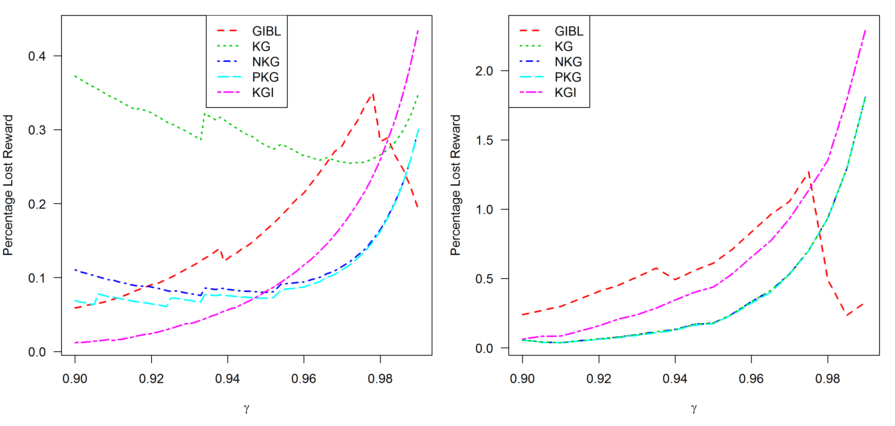
Figure 1: Mean percentage of lost reward compared to the GI policy for five policies for the Bernoulli MAB with uniform priors and $\gamma\in[0.9,0.99]$. The left plot shows $k=2$ while on the right $k=10$.

The overall behaviour of the policies is similar for $k=2$ and $k=10$. KGI is strong for lower $\gamma$ but is weaker for higher $\gamma$ while GIBL is strongest as $\gamma$ increases. The sharp change in performance for GIBL at $\gamma\approx 0.975$ occurs because the GIBL index is a piecewise function. Both NKG and PKG improve on KG for $k=2$ but the three KG variants are almost identical for $k=10$. The difference between KG and NKG gives the cost for the KG policy of dominated actions. These make up a large proportion of the lost reward for KG for lower $\gamma$ but, as $\gamma$ increases, over-greedy errors due to the myopic nature of the KG policy become more significant and these are not corrected by NKG. These errors are also the cause of the deteriorating performance of KGI at higher $\gamma$. At $k=10$ the states given in Section 3.3 where KG was shown to take dominated actions occur infrequently. This is because, for larger numbers of arms there will more often be an arm with $\mu\geq 0.5$ and such arms are chosen in preference to dominated arms.

However, states where $\mu<0.5$ for all arms will occur more frequently when arms have lower $\theta$. Here dominated actions can be expected to be more common. We can test this by using priors where $\beta>\alpha$. Figure 2 shows the effect of varying the $\beta$ parameter for all arms.

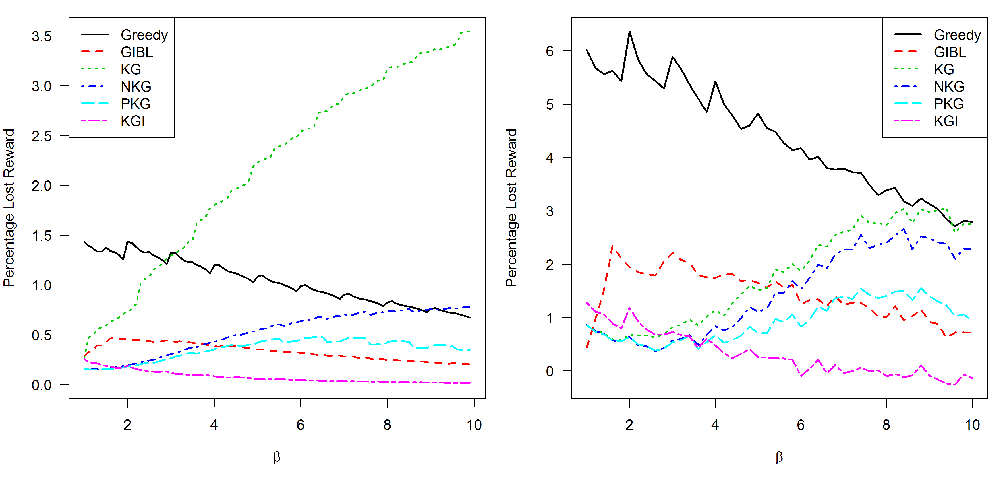
Figure 2: Percentage lost reward relative to the GI policy for six policies for the Bernoulli MAB with $\alpha=1,\beta\in[1,10]$ and $\gamma=0.98$. The left plot shows $k=2$ while on the right $k=10$.

The discount rate $\gamma=0.98$ is quite a high value where the greedy policy can be expected to perform poorly since exploration will be important. However as $\beta$ increases the performance of KG deteriorates to the extent that it is outperformed by the greedy policy. This effect is still seen when $k=10$. The superior performance of NKG shows that much of the loss of KG is due to dominated actions. Policy PKG improves further on NKG suggesting that KG makes further errors due to asymmetric updating even when it does not choose dominated arms. A clearer example of this is given in Section 5.3. Both policies based on GI approximations perform well and are robust to changes in $\beta$. KGI is the stronger of the two as GIBL is weaker when the rewards are less Normally distributed.

The same pattern can also be seen to be present when arms have low success probabilities but prior variance is high. Figure 3 gives results for $\beta=1$ with low $\alpha$. The range shown focuses on lower prior $\mu$ which correspond to $\beta\in[2,\ldots 50]$ in the setup of the previous experiment. The higher prior variance makes arms with higher success probabilities more likely than in the previous experiment but as $\alpha$ is reduced the performance of KG can still be seen to deteriorate markedly. The other policies tested do not show this problem.

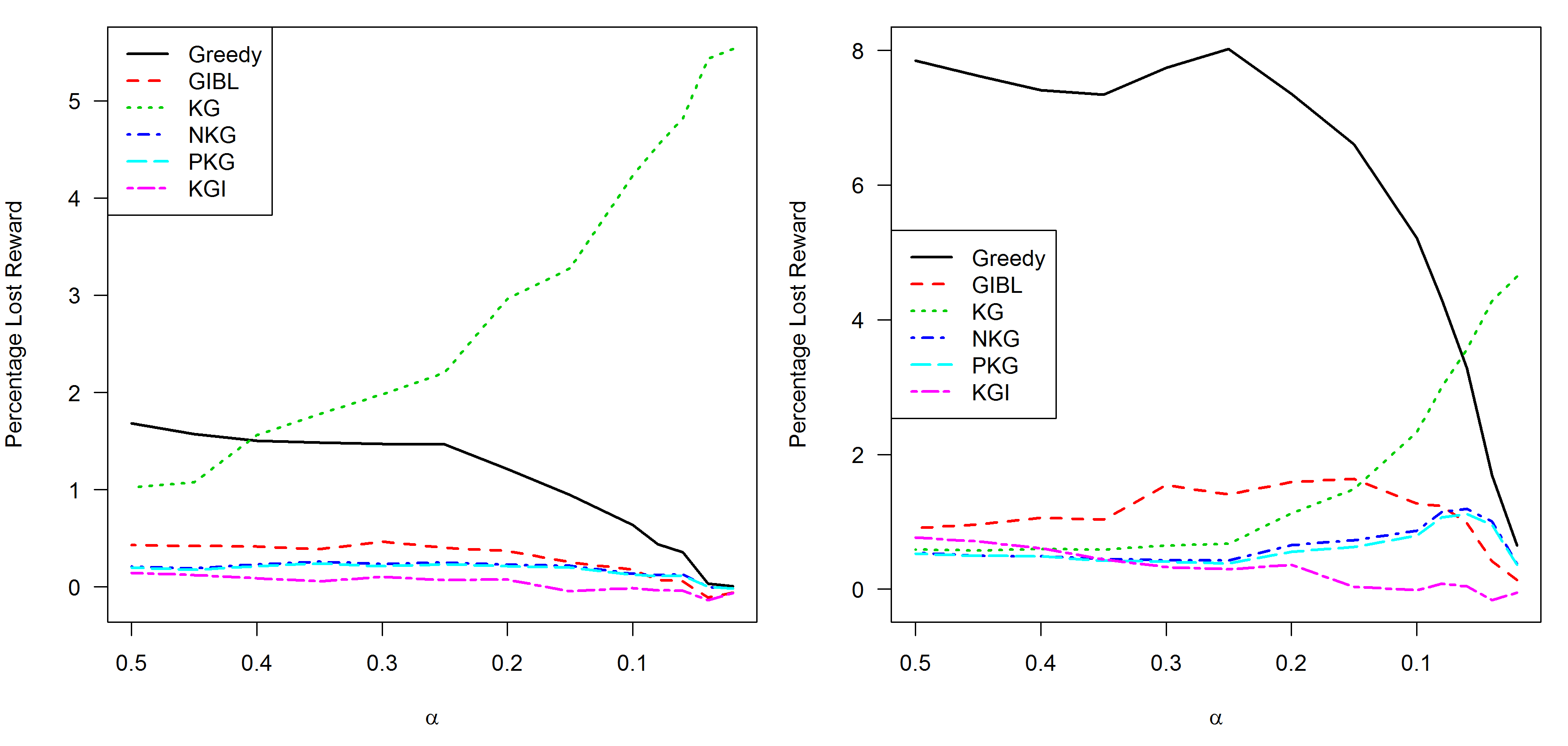
Figure 3: Percentage lost reward relative to the GI policy for six policies for the Bernoulli MAB with $\beta=1,\alpha\in[0.02,0.5]$ and $\gamma=0.98$. The left plot shows $k=2$ while on the right $k=10$.

Arms with low $\theta$ are common in many applications. For example, in direct mail marketing or web based advertising where $\theta$ is the probability that a user responds to an advert. The unmodified KG is unlikely to be an effective method in such cases.

The equivalent plots with prior $\mu>1$ do not show any significant changes in behaviour compared to uniform priors.

Another policy that is popular in the bandit literature and which has good theoretical properties is Thompson Sampling (e.g. Russo and Van Roy, [11]). Results for this method are not given in detail here as its performance is far inferior on these problems to the other policies tested. For example, on the results displayed in Figure 1 losses were in the ranges from $1.3-4\%$ and $6-15\%$ for $k=2$ and $k=10$ respectively with the best performance coming for $\gamma=0.99$. It is a stochastic policy and so makes many decisions that are suboptimal (including dominated errors). Its strength is that it explores well in the limit over time, eventually finding the true best arm. However, with discounted rewards or when the horizon is finite it gives up too much short term reward to be competitive unless $\gamma$ is close to 1 or the finite horizon is long. In addition, note that it will spend longer exploring as $k$ increases as it seeks to explore every alternative. Performance on the other problems in this paper was similar and so are not given.

5.3 Exponential MAB

This section gives the results of simulations for policies run on the MAB with Exponentially distributed rewards as outlined in Section 3.3. These are shown in Figure 4. Here the lost reward is given relative to the KG policy (the negative values indicate that the other policies outperformed KG). Different priors give a similar pattern of results.

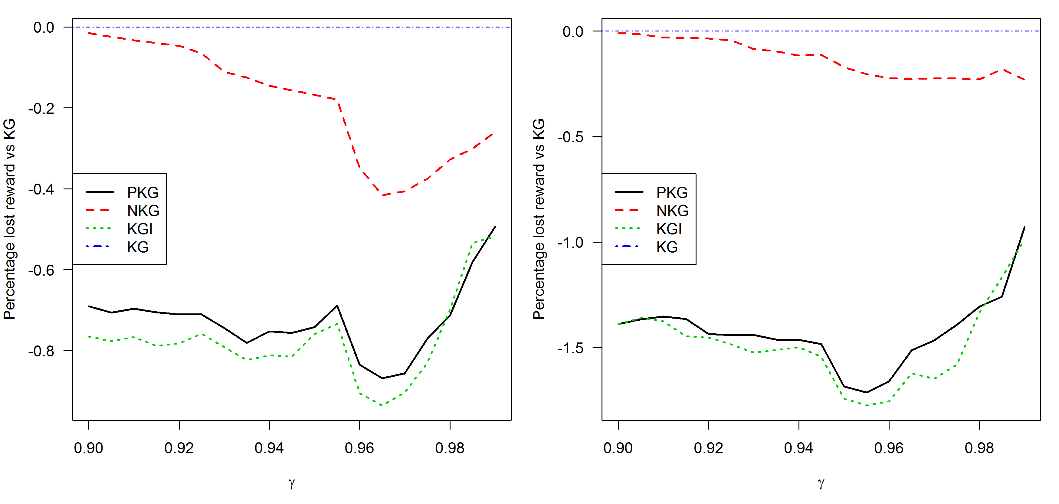
Figure 4: Mean percentage of lost reward compared to the KG policy for three policies for the Exponential MAB with Gamma(2,3) priors and $\gamma\in[0.9,0.99]$. The left plot shows $k=2$ while on the right $k=10$.

The results show a clear improvement over the KG policy by PKG and NKG policies. Notably the PKG earns better reward than the NKG indicating that the bias that causes dominated errors also causes suboptimal choices when arms are not dominated. Policy KGI gives the best performance although similar to PKG.

6 The Gaussian MAB

Here we consider the Gaussian case $Y_{a}\mid\theta_{a}\backsim N(\theta_{a},1)$ and $\theta_{a}\backsim N\left(\frac{\Sigma_{a}}{n_{a}},\frac{1}{n_{a}}\right)$. In the brief discussion in Section 3 we noted that KG does not take dominated actions in this case. While Ryzhov et al., [14] give computational results which demonstrate that KG outperforms a range of heuristic policies, the policy still makes errors. In this section we describe how errors in the estimation of arms’ learning bonuses constitute a new source of suboptimal actions. We also elucidate easily computed heuristics which outperform KG. A major advantage of KG cited by Ryzhov et al., [14] is its ability to incorporate correlated beliefs between arms. We will later show, in Section 6.1.3, that it is unclear whether KG enjoys a performance advantage in such cases.

We shall restrict the discussion to cases with $k=2$, $0<\gamma<1$ and $T=\infty$ and will develop a notion of relative learning bonus (RLB) which will apply across a wide range of policies for such problems. We shall consider stationary policies $\pi$ whose action in state $\left(\mathbf{\Sigma,n}\right)\equiv\left(\Sigma_{1},n_{1},\Sigma_{2},n_{2}\right)$ depends only upon the precisions $n_{b}$ and the difference in means $\Delta\mu:=\frac{\Sigma_{2}}{n_{2}}-\frac{\Sigma_{1}}{n_{1}}$. We shall write $\pi\left(\Delta\mu,n_{1},n_{2}\right)$ in what follows. We further require that policies be monotone in the sense of the following definition of the RLB.

Definition 14 (Relative Learning Bonus)

If $\pi$ is monotone in $\Delta\mu$ such that $\exists$ function $R^{\pi}:\mathbb{N}^{2}\rightarrow\mathbb{R}$ with $\pi\left(\Delta\mu,n_{1},n_{2}\right)=2\Leftrightarrow\Delta\mu\geq R^{\pi}\left(n_{1},n_{2}\right)$ $\forall\left(n_{1},n_{2}\right)$ then $R^{\pi}$ is the RLB function.

This monotonicity is a natural property of deterministic policies and holds for all policies considered in this section since increasing $\Delta\mu$ while holding $n_{1},n_{2}$ unchanged favours arm 2 in all cases. The RLB gives a method of comparing the actions of index and non-index policies but it is also useful when comparing index policies. A natural method of evaluating an index policy would be to measure the difference in its indices from GI in the same states. This can be inaccurate. An index formed by adding a constant to GI will give an optimal policy so it is not the magnitude of the bias that is important but how it varies. The RLB and the idea of index consistency (discussed later) give methods to assess this distinction.

Under the above definition we can set $\Sigma_{1}=0$ without loss of generality. We then have that $\Delta\mu=\mu_{2}$ and arm $2$ is chosen by policy $\pi$ in state $\left(\mathbf{\Sigma,n}\right)$ if and only if $\mu_{2}\geq R^{\pi}\left(n_{1},n_{2}\right)$. Figure 5 illustrates this for the GI and KG policies, the former of which determines the optimal RLB values. The plots are of slices through the $R^{GI}$ and $R^{KG}$ surfaces with $n_{1}=1$ and with $\gamma$ set at $0.95$. As $n_{2}$ increases the GI learning bonus for arm $2$ decreases, yielding values of $R^{GI}\left(1,n_{2}\right)$ which are increasing and concave. Comparison with the $R^{KG}\left(1,n_{2}\right)$ suggests that the latter is insufficiently sensitive to the value of $n_{2}$. This is caused by a KG value close to zero for arm $2$ when $n_{2}\geq 2$ and results in a mixture of over-exploration and over-exploitation. In practice when the priors of the two arms are close, over-exploration is the main problem. For $n_{1}>1$ the RLB curves have a similar shape but with smaller $R$ as the learning bonuses for both policies decrease with increased information over time.

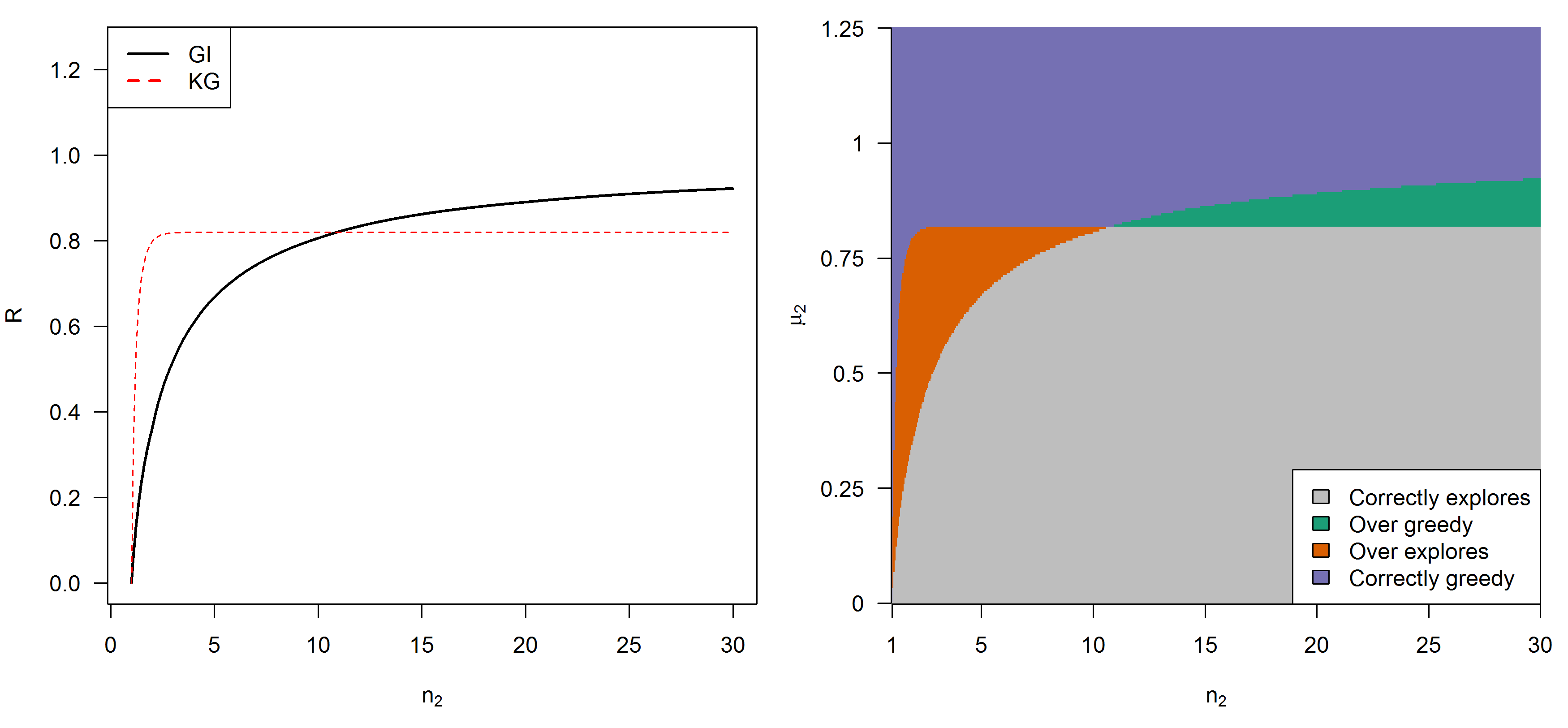
Figure 5: The left plot shows RLB values for KG and GI policies for $\gamma=0.95$, $n_{1}=1$, $\mu_{1}=0$. The right plot shows the nature of KG actions over different arm 2 states.

Figure 6 contains comparative plots of $R^{GI}\left(1,n_{2}\right)$ and $R^{\pi}\left(1,n_{2}\right)$ for three other policies $\pi$ and with $\gamma$ again set at $0.95$. The policies are KGI, described in Section 4, and two others which utilise analytical approximations to the Gittins Index, namely GIBL (Brezzi and Lai, [2]) and GICG (Chick and Gans, [3]). Although the latter use similar approaches to approximating GI their behaviour appear quite different, with GIBL over-greedy and GICG over-exploring. This changes when $\gamma$ is increased to $0.99$ where both policies over-explore. Although not shown here, the approximation of GI by both GIBL and GICG improve as $n_{1}$ increases and the corresponding RLB curves are closer. A suboptimal action is often less costly when over-greedy, especially for lower $\gamma$ since immediate rewards are guaranteed while the extra information from exploration might not yield any reward bonus until discounting has reduced its value.

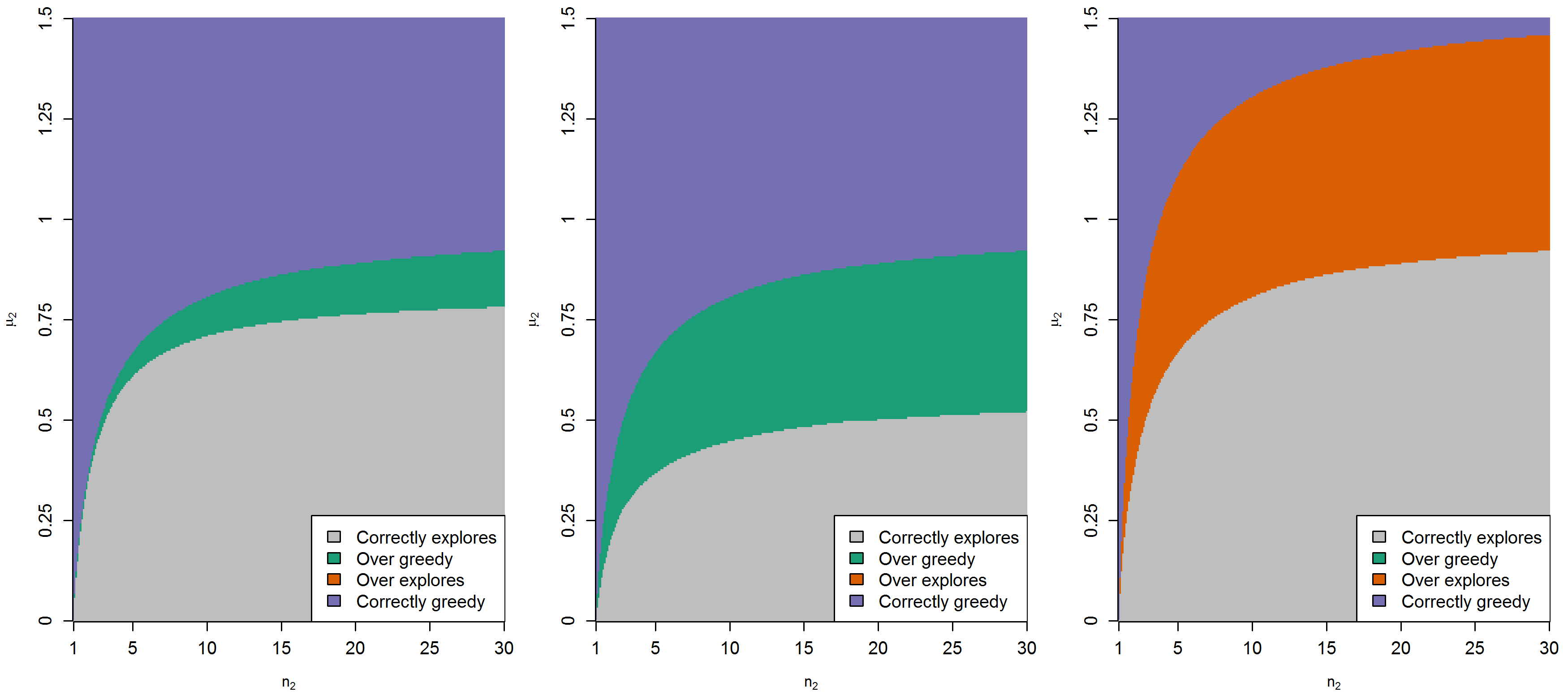
Figure 6: Plots of actions for KGI, GIBL and GICG (from left to right) for $\gamma=0.95$, $n_{1}=1$, $\mu_{1}=0$.

Weber, [16] enunciates a desirable property for policies which is enjoyed by the optimal GI policy. It can be thought of as a generalised stay-on-a-winner property.

Definition 15

A policy is index consistent if, once an arm is chosen then it continues to be chosen while its Gittins index remains above its value at the start of the period of continuation.

The region of over-exploration in the RLB plot in Figure 5 yields states in which KG is not index consistent. It will simplify the proof and discussion of the next result if we write the Gittins index for an arm in state $\left(\Sigma,n\right)$ as $\nu^{GI}\left(\Sigma,n\right)=\frac{\Sigma}{n}+l^{GI}\left(n\right),$ where $l^{GI}$ is the GI (ie, optimal) learning bonus for the arm. Note that for notational economy we have dropped the $\gamma$-dependence from the index notation. It now follows from the above definition that $R^{GI}\left(n_{1},n_{2}\right)=l^{GI}\left(n_{1}\right)-l^{GI}\left(n_{2}\right)$. More generally, if $\pi$ is an index policy we use $l^{\pi}$ for the learning bonus implied by $\pi,$ with $R^{\pi}\left(n_{1},n_{2}\right)=l^{\pi}\left(n_{1}\right)-l^{\pi}\left(n_{2}\right)$.

To prove Proposition 16 we use that each policy over-explores, as shown in Figures 5 and 6 for KG and GICG and for (e.g.) $\gamma=0.99$ for GIBL (not shown). The idea of the proof is that a policy that over-explores overestimates the RLB of the arm with lower $n$. After the arm is pulled $n$ increases and its RLB is reduced. There are values of $y$ such that the arm’s GI will increase (as its reduction in RLB is smaller) but its $\mu$ will not increase sufficiently to overcome the loss of RLB and so the policy will switch arms.

Proposition 16

Policies KG, GIBL and GICG are not index consistent.

• Proof. For definiteness, consider policy KG. From the calculations underlying Figure 5 we can assert the existence of state $\left(\mathbf{\Sigma,n}\right)$ such that $\Sigma_{1}=0,n_{1}=1,n_{2}=2$ and $2R^{KG}\left(1,2\right)>\Sigma_{2}>2R^{GI}\left(1,2\right)$, equivalently, $R^{KG}\left(1,2\right)>\mu_{2}>R^{GI}\left(1,2\right),$ when $\gamma=0.95$. It follows that $A^{KG}\left(\mathbf{\Sigma,n}\right)=1$ and KG over-explores in this state. We suppose that the pull of arm $1$ under KG in state $\left(\mathbf{\Sigma,n}\right)$ yields a reward $y$ satisfying $\mu_{2}>\frac{y}{2}>R^{GI}\left(1,2\right)=l^{GI}\left(1\right)-l^{GI}\left(2\right)$. But $\nu^{GI}\left(y,2\right)=\frac{y}{2}+l^{GI}\left(2\right)>l^{GI}\left(1\right)=\nu^{GI}\left(0,1\right)$ and so the Gittins index of arm $1$ has increased as a result of the reward $y$. However, the symmetry of the Normal distribution and the fact that $\mu_{2}>y$ guarantees that KG will choose arm $2$ in the new state. Thus while the Gittins index of arm $1$ increases, KG switches to arm $2$ and hence is not index consistent. Regions of over-exploration for GIBL and GICG (in the former case when $\gamma=0.99$) means that a similar argument can be applied to those policies. This concludes the proof.  

An absence of over-exploration does not guarantee index consistency for a policy. However, we now give a sufficient condition for an index policy never to over-explore and to be index consistent.

Proposition 17

If index policy $\pi$ satisfies $0\leq R^{\pi}\left(n_{1},n_{2}\right)\leq R^{GI}\left(n_{1},n_{2}\right)$ $\forall n_{1}<n_{2}$ then it never over-explores and is index consistent.

• Proof. Let state $\left(\mathbf{\Sigma,n}\right)$ be such that $\Sigma_{1}=0$. This is without loss of generality. For the over-exploration part of the result, we consider two cases. In case $1$ we suppose that $\mu_{2}>0$ and the GI policy chooses greedily when it chooses arm $2$. This happens when $\mu_{2}\geq R^{GI}\left(n_{1},n_{2}\right)$. If $n_{1}<n_{2}$ then the condition in the proposition implies that $\mu_{2}\geq R^{\pi}\left(n_{1},n_{2}\right)$ and policy $\pi$ must also choose arm $2$. If $n_{1}\geq n_{2}$ then the condition in the proposition implies that $R^{\pi}\left(n_{1},n_{2}\right)\leq 0$ and hence that $\mu_{2}\geq R^{\pi}\left(n_{1},n_{2}\right)$ trivially, which implies that policy $\pi$ continues to choose arm $2$. This concludes consideration of case $1$. In case $2$ we suppose that $\mu_{2}\leq 0$ and so the GI policy chooses greedily when it chooses arm $1$. If $n_{1}<n_{2}$ then we have $\mu_{2}\leq 0\leq R^{\pi}\left(n_{1},n_{2}\right)$ while if $n_{1}\geq n_{2}$ then we must have that $\mu_{2}\leq R^{GI}\left(n_{1},n_{2}\right)\leq R^{\pi}\left(n_{1},n_{2}\right)\leq 0$. Either way, policy $\pi$ also chooses arm $1$ and case $2$ is concluded. Hence, under the condition in the proposition, policy $\pi$ never explores when GI is greedy, and so never over-explores. For the second part of the result suppose that in state $\left(\mathbf{\Sigma,n}\right),$ index policy $\pi$ chooses arm $a$ and that the resulting reward $y$ is such that $\nu^{GI}\left(\Sigma_{a}+y,n_{a}+1\right)>\nu^{GI}\left(\Sigma_{a},n_{a}\right),$ namely arm $a$’$s$ Gittins index increases. Under the condition in the proposition we then have that

  $$\frac{\Sigma_{a}+y}{n_{a}+1} +l^{GI}\left(n_{a}+1\right)>\frac{\Sigma_{a}}{n_{a}}+l^{GI}\left(n_{a}\right)$$

  $$\Leftrightarrow\frac{\Sigma_{a}+y}{n_{a}+1}-\frac{\Sigma_{a}}{n_{a}}>R^{GI}\left(n_{a},n_{a}+1\right)\geq R^{\pi}\left(n_{a},n_{a}+1\right)$$

  $$\Rightarrow\frac{\Sigma_{a}+y}{n_{a}+1}+l^{\pi}\left(n_{a}+1\right)>\frac{\Sigma_{a}}{n_{a}}+l^{\pi}\left(n_{a}\right)$$ (6.1)

  and we conclude that policy $\pi$ will continue to choose arm $a$. Hence $\pi$ is index consistent. This concludes the proof.  

Conjecture 18

On the basis of extensive computational investigation we conjecture that policy KGI satisfies the sufficient condition of Proposition 17 and hence never over-explores and is index consistent. We have not yet succeeded in developing a proof.

6.1 Computational Study

This section gives the results of computational experiments on the MAB with Normally distributed rewards (NMAB). The same methodology as in Section 5 is used. As well as the basic MAB, also considered are the finite horizon NMAB with undiscounted rewards (Section 6.1.2) and a problem where arm beliefs are correlated (Section 6.1.3). It extends the experiments of Ryzhov et al., [14] by testing against more competitive policies (including GI) and by separating the effects of finite horizons and correlated arms. In both of these latter problems the Gittins Index Theorem (Gittins et al., [7]) no longer holds and there is no index policy that is universally optimal. This raises the question of whether index policies suffer on these problems in comparison to non-index policies such as KG.

A new parameter, $\tau$ for the observation precision is introduced for several of these experiments so that $Y_{a}\mid\theta_{a}\backsim N(\theta_{a},\tau)$. In Section 6 it was assumed $\tau=1$ but the results given there hold for general $\tau$. The posterior for $\theta$ is now updated by $p(\theta_{a}|y)=g(\theta|\Sigma_{a}+\tau y,n_{a}+\tau)$. We take $\tau$ to be known and equal for all arms.

6.1.1 Infinite Horizon, Discounted Rewards

The first problem compares KG, KGI, GIBL, GICG against the optimal policy on the standard NMAB over a range of $\tau$. The lost reward as a percentage of the optimal reward is shown in Figure 7.

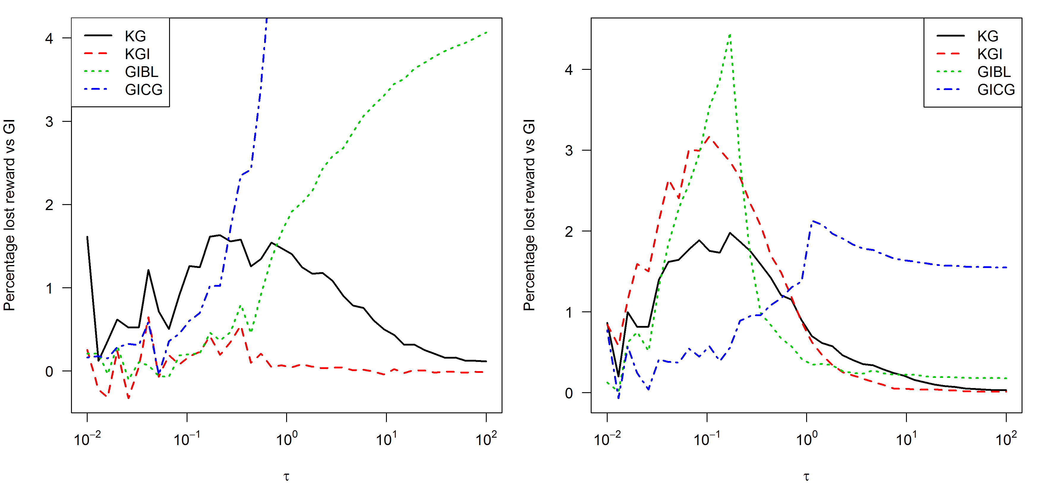
Figure 7: Lost reward versus optimal for heuristic policies for the NMAB with $\gamma=0.9$ (left) and $\gamma=0.99$ (right). There are $k=10$ arms each with a $N(0,1)$ prior.

The plot does not show the loss for GICG for high $\tau$ and $\gamma=0.9$ as it is very high relative to the other policies (rising to $>38\%$). The Greedy policy has similarly poor performance.

Ryzhov et al., [14] used the GICG policy as a comparator for the KG policy for the discounted Gaussian MAB. It was described as “the current state of the art in Gittins approximation”. These approximations are supposed to be better than the older GIBL but it appears that the improvements are mainly for large $n$ which may not result in improved performance. The RLB plots earlier in this section suggest that the approximations for low $n$ are not better and it is more important to be accurate in states reached at early times due to discounting. As $\gamma$ becomes larger these early actions form a smaller portion of total reward and are therefore less significant.

There is no one best policy for all problem settings. Policy KGI is uniformly strong for $\gamma=0.9$ but is weaker for $\gamma=0.99$. Both KGI and KG do well for high $\tau$. This is because more information is gained from a single observation and so myopic learning policies become closer to optimal. As $\tau$ becomes smaller it becomes important to consider more future steps when evaluating the value of information. However when $\tau$ is very low learning takes so long that a simple greedy approach is again effective. Hence KG and KGI are weakest for moderate values of $\tau$ between 0.1 and 1, depending on the number of arms.

6.1.2 The Finite Horizon NMAB

This section considers a variant on the NMAB where the horizon is a fixed length and rewards are not discounted (FHNMAB). One strength of KG is that it adapts easily for different horizon lengths and discount rates. GIBL and GICG, however, are designed only for infinite horizons. Ryzhov et al., [14] got round this problem by treating the discount rate as a tuning parameter. This allowed them to run experiments on a single horizon length ($T=50$). However, it is not ideal. Firstly, the tuning parameter will need to be different for different horizons and there is no simple way to set this. Secondly, the policy is not appropriate for the problem because a policy for a finite horizon should be dynamic, it should change over time by exploring less as the end time approaches, whereas this policy is static over time. We give a method here by which any policy designed for an infinite discounted problem can be adapted to a finite horizon one so that it changes dynamically with time. Note that all KG variants given in this paper (including KGI) are already dynamic when the horizon is finite so do not require any adjustment.

Definition 19 (Finite Horizon Discount Factor Approximation)

A policy which depends on a discount factor $\gamma$ can be adapted to an undiscounted problem with a finite horizon $T$ by taking

$$\gamma(t,T)=\frac{T-t-1}{T-t},\quad t=0,1,\ldots,T-1.$$ (6.2)

This chooses a $\gamma$ such that $\gamma/(1-\gamma)=T-1-t$ so that the ratio of available immediate reward to remaining reward is the same in the infinite case with $\gamma$ discounting (LH side) as the undiscounted finite case (RH side).

Figure 8 shows percentage lost reward versus KG for KGI and the adjusted GIBL (with KG shown as a straight line at zero).

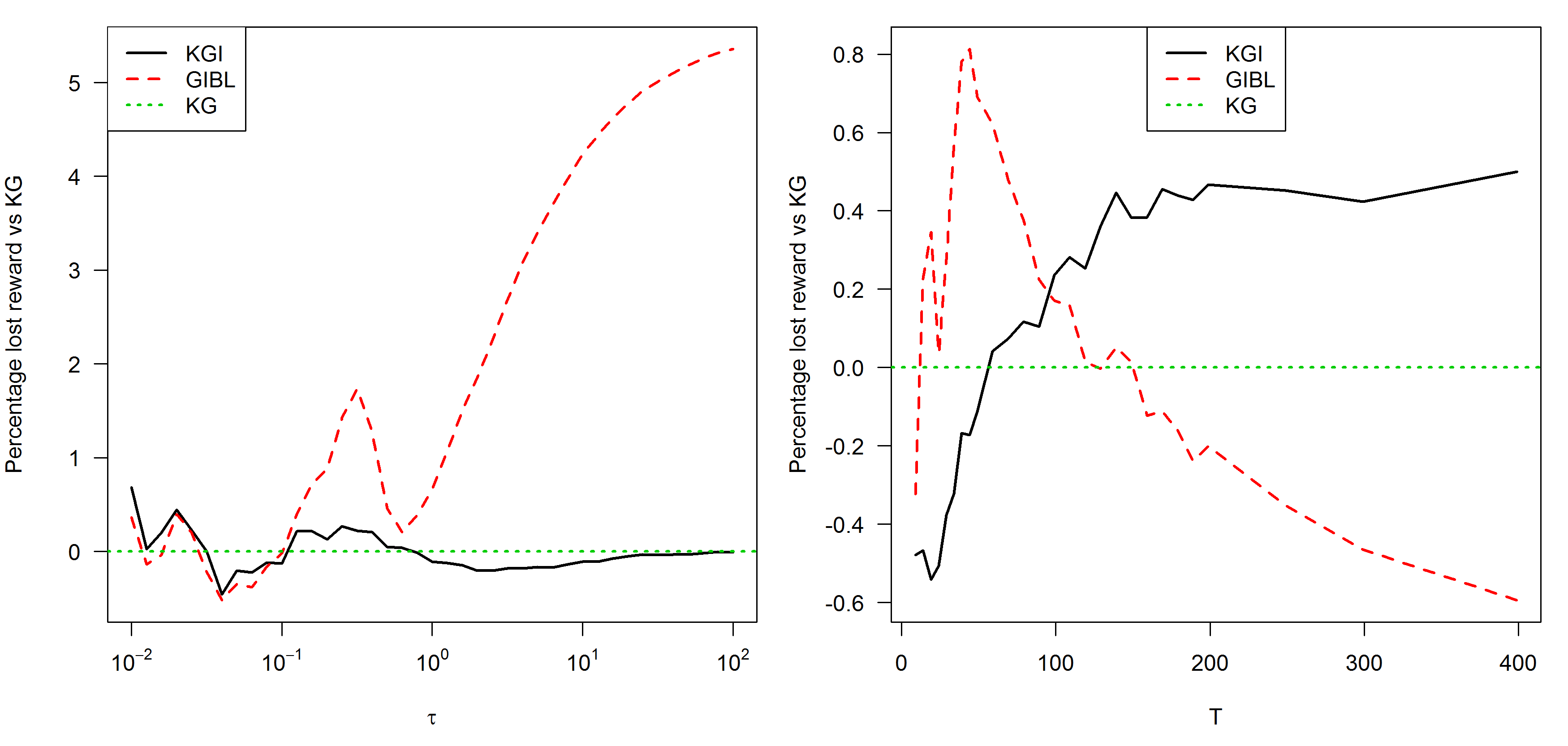
Figure 8: Lost reward on the FHNMAB. Left shows performance over a $\tau\in[10^{-2},10^{2}]$ with $T=50$, right over $T\leq 400$ with $\tau=1$. All $k=10$ arms had the same $N(0,1)$ prior.

Note that the scale of the vertical axis on the right plot is quite close to zero so that no policies are very distinct from KG here. GIBL shows similar behaviour to that seen in Figure 7 with infinite horizons, performing similarly to KG at $\tau=1$ (worse for shorter horizons but better for higher $T$) but doing very badly as $\tau$ increases above 1. KG and KGI show similar results but KG is the preferred policy for $T\geq 60$.

6.1.3 The Correlated NMAB

The NMAB variant where arm beliefs are correlated was studied in Ryzhov et al., [14] where the ability of KG to handle correlated beliefs was given as a major advantage of the policy. However, being able to incorporate correlation into the KG policy does not mean performance will improve and the experimental results that were given were mixed. A further short experimental study is conducted here for several reasons. Firstly, as shown earlier in this section, the GI approximation used (GICG) performs poorly in many circumstances and the GIBL and KGI policies might offer a stronger comparison. Secondly, Ryzhov et al., [14] used the finite horizon undiscounted version of the problem. As described earlier the policies based on GI are not designed for this problem so an artificial tuning parameter was introduced. Here we use infinite horizon with discounted rewards as before. This makes it clearer to see the effect of the introduction of correlation without the extra complication of the different horizon.

The problem is the same as the NMAB described in Section 6 except that beliefs are captured in a single multivariate Normal distribution for all the arms rather than one univariate Normal for each arm. For each simulation run the $\theta$ values for all arms are drawn from this true multivariate prior. The belief correlation structure can take many different forms but here we use the same the power-exponential rule used in Ryzhov et al., [14]. Prior covariances of the variance-covariance matrix $\boldsymbol{C}$ are

$$\boldsymbol{C}_{i,j}=e^{-\lambda(i-j)^{2}}.$$ (6.3)

where the constant $\lambda$ determines the level of correlation (decreasing with $\lambda$). In the experiments here all prior means are zero.

Two versions of KG are tested, the complete version that incorporates the correlation (CKG) and a version that assumes the arms are independent (IKG). Details of the CKG policy are given in Ryzhov et al., [14] using an algorithm from Frazier et al., [6]. All policies tested (including IKG) use the true correlated model when updating beliefs but, apart from CKG, choose actions that make the false assumption that arms are independent. Updating beliefs using the independence assumption results in much poorer performance in all cases and therefore these results are not shown. CKG is significantly slower than the other policies, scaling badly with $k$. This limits the size of the experiment so 40000 runs are used. The results over $\lambda\in[0.05,1]$ are shown in Figure 9.

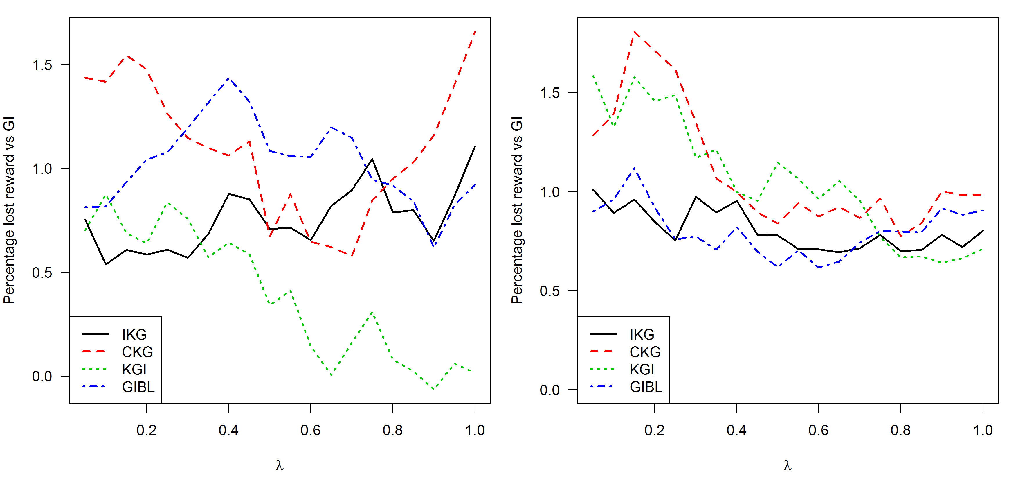
Figure 9: Lost reward vs GI on the Correlated NMAB for $\lambda\in[0.05,1]$ with $\gamma=0.9$ (left) and $\gamma=0.99$ (right). Both use $k=10$ with $\tau=1$.

The first observation is that, although GI is not optimal for this problem, it still clearly outperforms all the other heuristics indicating that using a index policy is not an obvious handicap. The GI approximation policies’ performance follows a similar pattern to the independent NMAB with KGI stronger at $\gamma=0.9$ and GIBL stronger at $\gamma=0.99$. IKG compares well to both these policies but again there is no evidence that non-index methods are stronger than index methods. More surprising is that CKG is clearly inferior to IKG. Frazier et al., [6] found CKG to be stronger in the offline problem but this does not appear to translate to the online problem. Exactly why this is so is not clear as this is a difficult problem to analyse. CKG requires $\mathcal{O}(k^{2}\log(k))$ to compute compared to IKG which requires $\mathcal{O}(k)$. CKG’s performance would have to be much better to justify its use and in many online problems with larger $k$ it would simply not be practical while IKG and the three simple index policies all scale well.

These experiments only scratch the surface of the correlated MAB problem and there are a number of possible issues. As rewards are observed the correlations in beliefs reduce and the arms tend to independence. Therefore correlations will be most important in problems with short horizons or steep discounting. Secondly, the number of arms used here is quite small. This is partly because CKG becomes very slow as $k$ increases so its use on larger problems would not be practical. A feature of correlated arm beliefs is that we can learn about a large number of arms with a single pull and therefore independence assumptions should be punished with greater numbers of arms. However we still learn about multiple arms as long as belief updating is handled accurately which is easy to do in this Gaussian setting. If this is not done then learning will be much slower and we did find that it is important that belief updating incorporates correlations.

One difficulty with analysing policies on this problem is that it still matters that the policy is effective on the basic MAB problem. Suboptimality in this regard can mask the effect of introducing correlation and changes may improve or worsen performance quite separately from addressing the issue of correlations. For example if a policy normally over-explores then any change that makes it greedier might improve performance. Thompson Sampling is a policy that can easily incorporate correlations (by sampling from the joint posterior) but the high level of exploration that comes from randomised actions does not do well on short horizon problems and any changes due to correlations will be too subtle to change that.

7 Conclusion

We identify an important class of errors, dominated actions which are made by KG. This involves choosing arms that have both inferior exploitative and explorative value. Much of the existing work on KG has focused on Gaussian rewards but these have features (symmetric and unbounded distributions) that avoid the domination problem. For other reward distributions the performance of KG can suffer greatly. Two new variants are given which remove this problem. Of these, NKG is simpler while PKG gives better experimental results by correcting errors besides those arising from dominated actions.

We also introduced an index variant of KG which avoids dominated actions, which we called KGI. For problems where the optimal policy is an index policy, simulation studies indicate that KGI is more robust than other proposed index policies that use approximations to the optimal index. It has computational advantages over KG and performed competitively in empirical studies on all problems tested including those where index methods are known to be suboptimal. One such problem is the MAB with correlated beliefs. Although KG can incorporate these beliefs it was found that any performance gain was, at best, small and did not justify the extra computation involved.

The new variants we introduce give a range of simple heuristic policies, of both index and non-index type. On the problems tested here at least, there did not appear to be any advantage to using non-index methods and, in addition, index methods have computational advantages on some BSDPs. However, this may not always be the case and further research will be needed to be more confident on other variants of this problem.

References

- Berry and Fristedt, [1985] Berry, D. A. & Fristedt, B. (1985). Bandit Problems. Chapman and Hall, London, UK.
- Brezzi and Lai, [2002] Brezzi, M. & Lai, T. L. (2002). Optimal learning and experimentation in bandit problems. Journal of Economic Dynamics and Control, 27(1):87–108.
- Chick and Gans, [2009] Chick, S. E. & Gans, N. (2009). Economic analysis of simulation selection problems. Management Science, 55(3):421–437.
- Ding and Ryzhov, [2016] Ding, Z. & Ryzhov, I. O. (2016). Optimal learning with non-Gaussian rewards. Advances in Applied Probability, 1(48):112–136.
- Frazier et al., [2008] Frazier, P. I., Powell, W. B., & Dayanik, S. (2008). A knowledge-gradient policy for sequential information collection. SIAM Journal on Control and Optimization, 47(5):2410–2439.
- Frazier et al., [2009] Frazier, P. I., Powell, W. B., & Dayanik, S. (2009). The knowledge-gradient policy for correlated normal beliefs. INFORMS Journal on Computing, 21(4):599–613.
- Gittins et al., [2011] Gittins, J. C., Glazebrook, K. D., & Weber, R. (2011). Multi-armed bandit allocation indices. John Wiley & Sons, Chichester, UK, second edition.
- Gupta and Miescke, [1996] Gupta, S. S. & Miescke, K. J. (1996). Bayesian look ahead one-stage sampling allocations for selection of the best population. Journal of Statistical Planning and Inference, 54(2):229–244.
- Jones et al., [1998] Jones, D. R., Schonlau, M., & Welch, W. J. (1998). Efficient global optimization of expensive black-box functions. Journal of Global Optimization, 13(4):455–492.
- Powell and Ryzhov, [2012] Powell, W. B. & Ryzhov, I. O. (2012). Optimal learning. John Wiley & Sons, Hoboken, NJ.
- Russo and Van Roy, [2014] Russo, D. & Van Roy, B. (2014). Learning to optimize via posterior sampling. Mathematics of Operations Research, 39(4):1221–1243.
- Ryzhov et al., [2010] Ryzhov, I. O., Frazier, P. I., & Powell, W. B. (2010). On the robustness of a one-period look-ahead policy in multi-armed bandit problems. Procedia Computer Science, 1(1):1635–1644.
- Ryzhov and Powell, [2011] Ryzhov, I. O. & Powell, W. B. (2011). The value of information in multi-armed bandits with exponentially distributed rewards. In Proceedings of the 2011 International Conference on Computational Science, pages 1363–1372.
- Ryzhov et al., [2012] Ryzhov, I. O., Powell, W. B., & Frazier, P. I. (2012). The knowledge gradient algorithm for a general class of online learning problems. Operations Research, 60(1):180–195.
- Shaked and Shanthikumar, [2007] Shaked, M. & Shanthikumar, J. G. (2007). Stochastic orders. Springer, New York.
- Weber, [1992] Weber, R. (1992). On the Gittins index for multiarmed bandits. The Annals of Applied Probability, 2(4):1024–1033.
- Whittle, [1980] Whittle, P. (1980). Multi-armed bandits and the Gittins index. Journal of the Royal Statistical Society. Series B (Methodological), 42(2):143–149.
- Whittle, [1988] Whittle, P. (1988). Restless bandits: Activity allocation in a changing world. Journal of Applied Probability, 25:287–298.
- Yu, [2011] Yu, Y. (2011). Structural properties of Bayesian bandits with exponential family distributions. arXiv preprint. arXiv:1103.3089v1.