Main Physical Aspects of the Mathematical Conception of Energy in Thermodynamics

Abstract

We consider the main physical notions and phenomena described by the author in his mathematical theory of thermodynamics. The new mathematical model yields the equation of state for a wide class of classical gases consisting of non-polar molecules provided that the spinodal, the critical isochore and the second virial coefficient are given. As an example, the spinodal, the critical isochore and the second virial coefficient are taken from the Van-der-Waals model. For this specific example, the isotherms constructed on the basis of the author’s model are compared to the Van-der-Waals isotherms, obtained from completely different considerations.

Keywords: Van-der-Waals model; compressibility factor; spinodal; number of degrees of freedom; admissible size of clusters; quasi-statical process.

1 Introduction

In the present paper, we present the foundations of the new mathematical model of thermodynamics for the values of the energy for which the molecules are in the pre-plasma state, in particular as pressure $P$ is near-zero.

The new mathematical model constructed by the author in the cycle of papers [1]–[2], differs somewhat from the commonly accepted model of phenomenological thermodynamics and allows us to construct the equation of state for a wider class of classical gases.

We mainly study the metastable states in the case of gases and in the case of fluids up to the critical isochore $\rho=\rho_{c}$. The liquid isotherms are divided into two parts: the region with temperatures near the critical temperature $T_{c}$ and the region of the “hard” liquid whose isotherms pass through the point of zero pressure.

Further, the distributions in the Van-der-Waals model are compared to the distributions appearing in the author’s new model for classical gases with given critical temperatures, in particular, with Van-der-Waals critical temperature. The precision with which the isotherms constructed from the author’s theory coincide with the Van-der-Waals isotherms turns out to be less than the accepted precision in experimental studies. The probability of such a coincidence being accidental is “infinitely small”.

All the distributions of energy levels for classical gas considered in the present paper have been established mathematically, see [1]–[3] and references therein) and have met with approval (see, for example, the review [4], published in the journal “Probability Theory and its Applications” in connection with the State Prize of the Russian Federation in Science and Technology granted to the author in 2013 (for developing the mathematical foundations of modern thermodynamics).

2 Van-der-Waals Normalization and the Law of
Corresponding States

The correct choice of units of measurement for different gases allowed Van-der-Waals to compare the parameters of the gases to dimensionless quantities, thus obtaining the famous “law of corresponding states”.

For every gas, there exists a critical temperature $T_{c}$ and a critical pressure $P_{c}$ such that if the temperature or the pressure is greater than their critical values, then gas and liquid can no longer be distinguished. This state of matter is known as a fluid.

The Van-der-Waals “normalization” consists in taking the ratio of the parameters by their critical value, so that we consider the reduced temperature $T_{r}=T/T_{c}$ and the reduced pressure$P_{r}=P/P_{c}$. In these coordinates, the diagrams of the state of various gases resemble each other – this a manifestation of the law of corresponding states.

The equation of state for the Van-der-Waals gas in dimensionless variables has the form:

$$(P_{r}+\alpha\rho^{2})(1-\tilde{\alpha}\rho)=\rho T_{r},$$ (1)

where $\alpha={3^{3}}/{2^{6}}$, $\tilde{\alpha}={1}/{2^{3}}$, and the dimensionless concentration (density) $\rho=N/V$ is chosen so that $\rho_{c}=8/3$ in the critical point.

In thermodynamics, the dimension of the internal energy $E$ is equal to the dimension of the product $PV$ of the pressure by the volume. On the other hand, temperature plays the role of mean energy $E/N$ of the gas (or of the liquid). For that reason, when the dimension of temperature is given in energy units, the parameter $Z=P/\rho T$, known as the compressibility factor, is dimensionless. For the equation of state of the gas or liquid, the most natural diagram is the $P_{r}$-$Z$ diagram, in which the dimensionless pressure $P_{r}$ is plotted along the $x$-axis and the dimensionless parameter $Z$, along the $y$-axis. A diagram with axes $P_{r},Z$ is called a Hougen–Watson diagram. In the Van-der-Waals model, the critical value of the compressibility factor is

$$Z_{c}=\frac{P_{c}V_{c}}{NT_{c}}=\frac{3}{8}.$$

In Figs. 2–1, the Van-der-Waals isotherms are shown in a $P_{r}$-$Z$ Hougen–Watson diagram, for which we used the normalization $P_{r}=P/P_{c}$, $T_{r}=T/T_{c}$, where $T_{c}$ is the critical temperature.

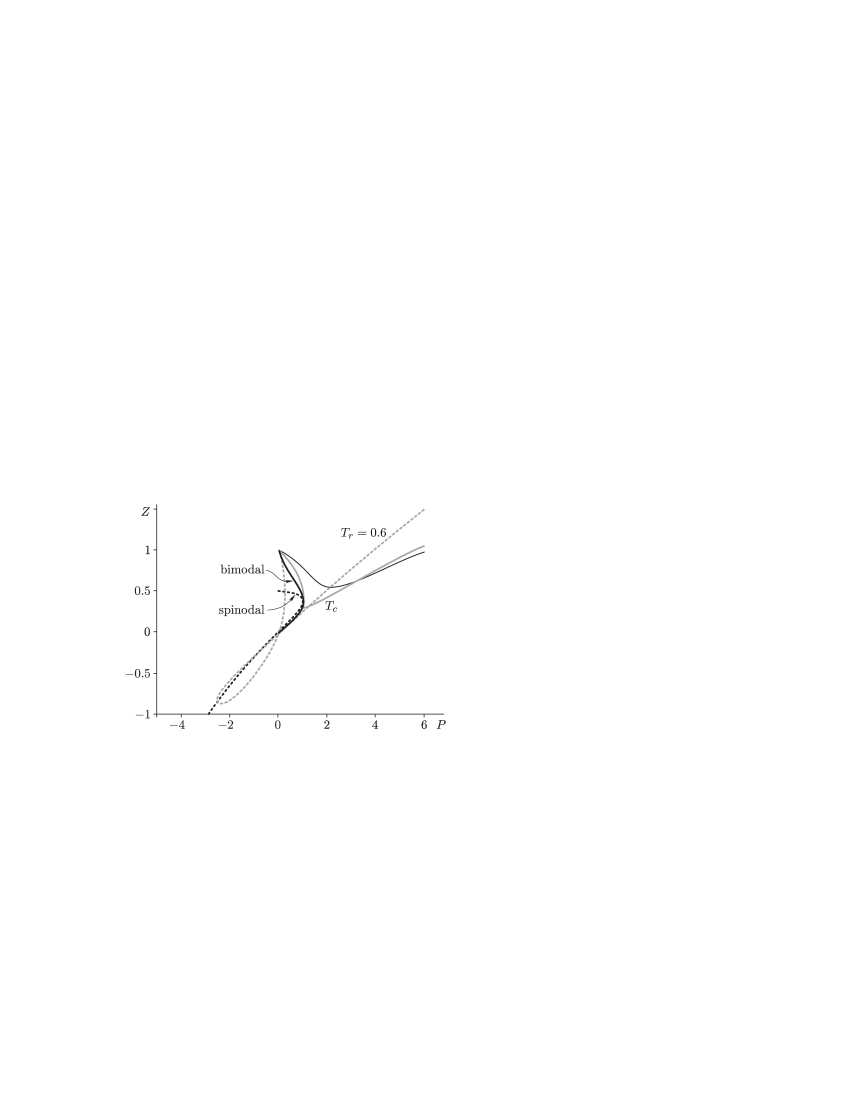
Figure 1: Van-der-Waals isotherms on the $P_{r}$-$Z$ diagram. On the plot $P=P_{r}$, $T=T_{r}$. The curve shown by the fat hashed line is the critical isotherm $T_{r}=1$. The dotted line is the spinodal, the thin hashed line is the binodal.

.

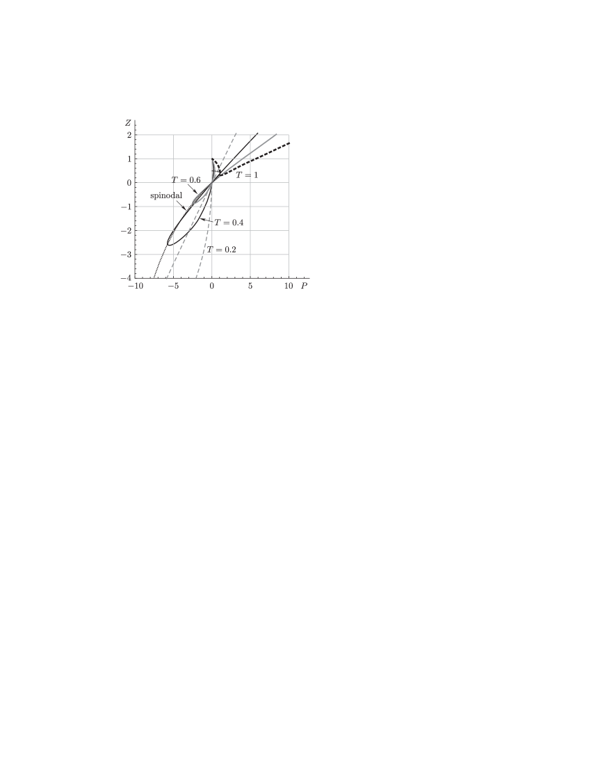
Figure 2: The $P_{r}$-$Z$ diagram for the Van-der-Waals equation with $P=P_{r}$.

3 On the Number of Degrees of Freedom and the Parition Theory of Integers

In the physics literature, the notion of number of degrees of freedom is used for ideal gases, in which particles do not interact. In probability, the number of degrees of freedom is also considered independently of any interaction.

When physicists speak of the number of degrees of freedom, they usually have in mind the number of degrees of freedom of a single molecule. Normally, a one-atom molecule will have 3 degrees of freedom, a two-atom molecule, 5. In a gas, the molecules move with different speeds and different energies; although their mean energy – temperature – is the same, their individual energies may be different, and the number of degrees of freedom of different molecules can also differ. Thus a two-atom molecule with very high energy may have a number of degrees of freedom greater than than 5, and this will affect the mean value (average over all molecules) of the number of degrees of freedom of the given gas. This mean value is called the collective number of degrees of freedom of the gas, and is a fractional rather than a whole number.

A one-atom molecule has 3 degrees of freedom, a two-atom molecule, 5. Two-atom molecules are regarded in [5] as molecules of ideal gas. Nevertheless, saying that the number of degrees of freedom of a molecule is 5 means that we are implementing an exclusion rule: we are saying that one of the degrees of freedom is excluded. More precisely, we regard the molecule as a dumbbell, and exclude its oscillations as a rod. However, if the temperature increases, these “rod” oscillations will take place and so, for sufficiently high temperatures (energies), the molecules will have a greater fractional number of degrees of freedom.

In the author’s model, the number of degrees of freedom is an important independent parameter, so that the notion of exclusion need not be defined by means of some internal considerations .

Although the collective number of degrees of freedom of a classical gas can be determined by the initial interaction between its particles, in the probabilistic description of the generalized ideal gas (a notion that we present in Section 5), this parameter is introduced independently.

If nuclear forces are taken into consideration, it can be shown that a wide class of two-atom molecules have 5 degrees of freedom, but this is difficult to establish. And so we prefer to stipulate axiomatically, as in probability theory, that on a given energy level there can be only one or, say, no more than $K$ particles.

Another important consideration is that we do not take into account the number of particles and the volume separately, we consider their ratio – density (concentration).

The consideration of density alone leads to the following important consequence in thermodynamics: density does not depend on the numeration of particles contained in the given volume. Whatever the numeration of the particles, the density remains the same. It is commonly believed (in particular, it is stated in the book [7]) that classical particles differ from quantum particles in that they can be numbered and then the motion of any individual particle can be followed by keeping track of its number. This is correct, but if the behavior of a multi-particle system is described by equations involving density, e.g. via a probability distribution, then such a description does not depend on the numbering of particles.

Therefore, all the results from quantum mechanics that follow from the remarkable fact that the solution does not depend on numeration can be carried over to the description of any classical multi-particle system by means of equations containing density.

As an illustrative example, we consider the purchase of 1 kilogram of granulated sugar. If this amount of sugar is measured by calculated the grains (and thus the grains must be first numerated), then it is obvious that this process takes a lot of time. Assume that the buyer has a fixed time for the measurement $t_{mes}$ which is equal to one hour and there is no balance to weight the sugar. Then the buyer will measure the granulated sugar by using some vessels. The results of weighting and of measuring by vessels does not change if two grains in the measured volume interchange their places. This means that (1) the particle identity principle holds for the sugar grains and (2) the sum of particles is independent of their location, i.e., the arithmetic property is satisfied [9]. In particular, this implies that one can use a Bose–Einstein-type distribution in this “classical” situation.

The exclusions that we impose will lead us to a more general distribution in which we stipulate that no more than $K$ particles are on the same energy level. The natural number $K$ will be called the maximal occupation number or maximal admissible size of clusters.

The corresponding energy distribution, often called parastatistical [10]–[11], will be described in the next sections. To specific and generalize the parastatistical distributions, we shall use the above-listed items (1) and (2).

Remark 1.

In the Landau–Lifshits textbook [5], two relations are given as the basic equations

$$\sum_{j}N_{j}=N,$$ (2)

$$\sum_{j}\varepsilon_{j}N_{j}={M},$$

where ${M}$ is the energy, $N$ is the number of particles and $\{\varepsilon_{j}\}$ is a discrete family of energy levels (see [12], [13]).

The values $\varepsilon_{j}$ in Eq. (2) are related to the existing interaction potential for the particles. It turns out that if we use the interaction with collective number of degrees of freedom equal to $D$, then we must put

$$\varepsilon_{j}=\text{const}\cdot j^{D/2},$$ (3)

i.e.,

$${M}=\sum_{j}\text{const}\cdot j^{D/2}N_{j}.$$ (4)

This statement is a theorem proved in the author’s paper [14].

The first person who noticed the unexpected relationship between the partition problem in number theory (in particular the famous discovery of Ramanujan) and nuclear disintegration, was Niels Bohr, the founder of quantum theory (see [15]).

It is well known that Bohr’s most famous opponent was the great Albert Einstein himself. The polemic between Bohr and Einstein, during which Bohr gave convincing answers to all of Einstein’s counterarguments, only fortified Bohr’s position and helped him in developing his quantum approach. In a commentary to one of Einstein’s letters, Max Born wrote: “… Einstein’s attitude to quantum mechanics was a heavy blow to me, he refuted the theory without any argumentation, only referring to his ‘inner voice’…” [16]. It was only after the experimental corroboration of the disintegration of heavy Lithium [17] and Uranium-235 that Einstein did support, albeit reluctantly, the A-bomb project.

The Bohr–Kalckar paper [18] of 1937 was the first work in which the coincidence of “thermodynamical formulas” with the number-theoretic formulas for partitions of integers into sums was discovered. Here is a quotation from that paper. “Under the simplifying assumption that each level is the combination of a certain number of quantities assuming nearly equidistant values, one can easily calculate the density of nuclear levels under high perturbations. Denote by $p(M)$ the number of possible ways of presenting a positive integer as a sum of smaller positive integers. An asymptotic formula for $p(M)$ was obtained by G. Hardy and S. Ramanujan. For large values of $M$ this formula may be approximately written in the form

$$p(M)\sim\frac{1}{4\sqrt{3}M}e^{\pi\sqrt{\frac{2}{3}M}}.$$

Let us choose $2\cdot 10^{5}eV$ for the unit of energy, which approximately corresponds to the common distance between the lowest levels of the heavier nuclei. For the number of partitions for which the perturbation energy of $8\cdot 10^{6}eV$ will be obtained, we will then find $p(M)\sim 2\cdot 10^{4}$. This means that the mean distance between levels approximately equals $10eV$, which roughly corresponds to the densities of distribution of levels calculated from the collisions of slow neutrons. $\langle\dots\rangle$ The formulas for the density of nuclear levels obtained by analogy with thermodynamics practically coincide, at least in the exponential dependence on the total energy of excited nuclei, with the formula for $p(M)$ if one understands the number $M$ as the measure of total energy expressed as the difference of energies between the lowest levels taken for the unit of measure” (see pp. 337–338 in the Russian translation [18]).

Bohr’s and Kalckar’s considerations about the distance between lowest energy levels is correct, because for the Schrödinger equation, the equations of the lower levels in the potential trough are quadratic.

Note that the probability of the coincidences indicated by Bohr and Kalckar being accidental is practically zero.

Later Bohr proposed using Uranium-235 as an example of the nucleus of an atom, since it was most appropriate for his construction and used it to explain how to generate a nuclear reaction [19].

The historian and archivist of the British Committee for Atomic Energy Margaret Going, on the basis of her study of the opinions of authoritative physicists, wrote: “… The work of English and American scientists on the A-bomb came directly from articles of Professor Bohr and Doctor Wheeler…”. Thus we may conclude that the creation of the A-bomb was based on the fantastic discovery of Ramanujan.

An essential role in establishing the new world outlook in physics was played by the numerous volumes of the famous treatise by Landau and Lifshits, in particular, [5] and [20]. In the book [5] in Section 40 “Nonequilibrium ideal gas,” the authors present the system of equations (2) and (3)–(4), on which their further exposition is based. Both $N$ and $N_{j}$ in these equations are integers. And so equations (2) coincide with the Diophantine equations for partitions in number theory. In the subsequent sections of the book [5] the main equations of thermodynamics are obtained without appealing to the so-called three main principles of thermodynamics, which appear in all textbooks on thermodynamics, but not in [5].

Bohr’s paper [18] generated only a trickle of mathematical and physical papers, in which the connection between the statistics of Bose–Einstein and Fermi–Dirac and the Ramanujan formula was studied in more detail [22]–[24]. Thus papers on this topic appeared in the mathematical journal “Mathematical Proceedings of the Cambridge Philosophical Society.” It was shown that if one takes into account the connections with partition theory, the Ramanujan formula and the Hardy–Ramanujan theorem in number theory, then it becomes clear that, in the case when there are repeated summands in the partition, the leading term of the Ramanujan formula coincides with the entropy of the Bose–Einstein statistics, whereas in the case when there are no repeated summands, this term coincides with the Fermi–Dirac entropy (bosons and fermions – no other particles are observed). Apparently, one of the last papers in this series is [24]. It contains a bibliography of the topic. But overall it seems that contemporary physicists did not pay attention to that series of papers and forgot that they are indebted to Ramanujan for the remarkable revolution in the scientific world outlook.

It follows from Bohr’s paper that his model of the nucleus of an atom does not involve the interaction of particles in the form of attraction. When Bohr visited the USSR in 1961, he demonstrated a simple model of a nucleus consisting of little balls in a cup. Several balls were placed in a cup, and then another little ball, endowed with a certain energy, was slipped into the cup. Were the cup empty, the new ball would have slipped out of the cup, but it shared some of its energy with the other balls and stayed in the cup. This is due to the fact that all the balls were in a common potential field. Thus Bohr regarded the nucleus as consisting of particles that do not attract each other.

Bohr’s model of the nucleus is a model without attraction of molecules, and so is Frenkel’s model of liquid (liquid drop model). Such a model of the nucleus appears to contradict the physical viewpoint as well as the commonsense (or naive) point of view. Nevertheless, it adequately describes nuclear fission, and Frenkel’s model adequately describes the behavior of liquids. The Frenkel model contains “holes” but does not involve mutual attraction of molecules.

Incidentally, Frenkel subtly complained about the difficulties of overcoming traditional viewpoints, using the word “we,” i.e. “physicists.” He writes: “We easily get used to uniform and steady things, we stop noticing them. What is habitual seems understandable, but we don’t understand the new and unusual, it seems unnatural and obscure $\langle\dots\rangle$. Essentially, we never really understand, we can only get used to” [25, p. 63]. If we follow Bohr, we see that in the thermodynamics that he talks about (see above), there is no attraction between molecules, but there is a common potential, in particular the Earth’s gravitational attraction. Molecules can collide, as they do in ideal gas, but there is no mutual attraction.

In Bohr’s paper mentioned above, he noted the connection between nuclear fission and the theory of partitions in number theory. On the other hand, he proposed the drop liquid model of the nucleus. This leads us to the idea that the theory liquids is also connected to partition theory. In that connection Bohr writes only about the analogy with thermodynamics, and so, like his pupil Landau, this means that they did not have in mind the old thermodynamics based on the “three fundamental principles,” but the thermodynamics understood in the framework of the new world outlook based on Bohr’s quantum theory postulates and partition theory.

The author, following the way traced out by Bohr and Landau, has developed a mathematical approach based on number theory problems and quantum theory. In the author’s model there is no attraction between particles, but there is a common potential, in particular, the potential due to the Earth’s gravitation and its rotation.

The author has shown that his approach to thermodynamics yields the same formulas as partition theory with logarithmic precision (which means the formulas coincide from the point of view of tropical arithmetic). The notion of logarithmic accuracy was introduced in Vol. X of the Landau–Lifshits textbooks [20] on p. 211. It is defined as follows: logarithmic accuracy of $M$ means that we find $M$ not up to $o(M)$, but only up to $o($ln$(M)$.

Before passing to the formulation of the main formulas and results, we recall the notions of tropical arithmetic and logarithmic accuracy.

The arithmetics of a system may be decimal or binary. The well-known notion of integer part of a real number, entier, is denoted by square brackets: $[a]$ stands for the maximum integer that does not exceed a given real number $a$. It is this integer that is usually retained in human memory. For example, although the number $2.99$ is close to $3$, our memory retains its integer part $2$; this peculiarity is used by marketing people when assigning prices to commodities in shops.

From the viewpoint of arithmetics, it is quite natural to discard the fractional part for sufficiently large $a$. If the numbers are as large as is common for macroscopic systems, it is convenient to use a generalization of this notion for large numbers. By $[a]_{10}$ we denote decimal arithmetics, where $[\cdot]_{10}$ means the same entier for rationals but with respect to $10$. For example, $[15]_{10}=10$, $[90]_{10}=10$, $[105]_{10}=100$, and $[6\cdot 10^{23}]_{10}=10^{23}$.

For the sum, we have $[10^{15}+10^{14}]_{10}=10^{15}$; i.e., the sum equals $\max(10^{15},10^{14})$. For the product, $10^{15}\cdot 10^{14}=10^{29}$; i.e., the product is equal to the number of zeros in a multidigit number.

Similar rules hold for a system considered in the binary arithmetics $[a]_{2}$.

The arithmetics thus constructed not only corresponds to the $(\max,+)$-algebra but also takes into account precision and neglects $c$-numbers, just as it happens in the Maslov–Litvinov dequantization. Hence we can say that this arithmetics is “tropical.”

For the natural logarithm, we deal with a special situation. Here we must use the great formula due to the great Ramanujan and the natural logarithm of the solution given by this formula. By considering the integer parts $[\log_{e}p(M)]$, we obtain a partition of $p(M)$ into similar subsets of integers.

Note that the use of the natural logarithm is natural if the formulas use the polylogarithm, because the polylogarithm emerges from the Stirling formula, and the Stirling formula contains Euler’s number $e$.

Thus, in addition to the arithmetics described by the entiers $[\cdot]_{10}$ and $[\cdot]_{2}$, we introduce the arithmetics $[\cdot]_{e}$ on the basis of partition theory.

Definition 1.

We say that two numbers coincide with logarithmic accuracy if the values of their normal arithmetics $[\cdot]_{e}$ coincide. In other words, $\ln A\cong\ln B$ means that $\ln A=\ln B+o(\ln B)$.

Since this arithmetics puts all elements coinciding with each other with “logarithmic accuracy” into the same equivalence class, we see that convergent series are equivalent to polynomials. It follows that, to each series $\Phi$, we can assign the degree of the corresponding polynomial. We denote this number by $n(\Phi)$. If one can assign an enveloping series to a divergent series, then the minimum number of the enveloping series naturally determines the degree $n(\Phi)$ of the corresponding polynomial.

Now we can briefly present a classical problem in partition theory of integers renewed by the inclusion of the number zero and negative entropy (negentropy).

First, consider some examples.

Example 1.

If we partition the number 5 into 2 summands, zero summands not allowed, then we obtain $p_{N}(M)=2$, 5=4+1=3+2, where $N$ is the number of summands, $N=1,2,\dots,M$, and $p_{N}(M)$ is the number of partitions of $M$ into $N$ summands. There are two possible partitions in this example for $N=2$.

Example 2.

Let us allow zero summands in partitions of $M$ into $N$ summands. Then $p_{N}(5)=3$ for $N=2$ in the preceding example, 5=5+0=4+1=3+2. All in all, there are three possible partitions in this case.

When partitioning 5 into 3 with zeros allowed, the $p_{N}(M)$ partitions without zeros, $5=3+1+1=2+2+1=\dots$ , are supplemented with partitions containing zeros, $4+1+0=3+2+0=5+0+0$. With zeros taken into account, all preceding partitions are repeated; i.e., we obtain the sum of all partitions without zeros.

We introduce the following notation:

$\bar{p}_{s}(M)=\sum_{i=1}^{s}p_{i}(M)$.

Proposition 1.

The number of partitions of $M$ into $N$ summands, zero summands allowed, coincides with $\bar{p}_{s}(M)$ for $s=N$.

Definition 2.

Let $q_{N}(M)$ be the number of partitions of $M$ into $N$ distinct summands, and let

$$q(M)=\sum_{N}q_{N}(M).$$

By definition, the partition 3+1+1 of 5 into 3 terms is excluded from $q_{N}(M)$. All the zeros are excluded as well.

Let us continue the partition $\bar{p}_{N}(M)$ by the numbers $q_{N}(M)$. This continuation is continuous, because for $M=1$ there are two partitions, $M=1=1+0$, taken into account in $\bar{p}_{N}(M)$ and one partition, $q_{N}(1)=1$, taken into account in $q_{N}(M)$.

We define natural entropy as the natural logarithm of $\bar{p}_{N}(M)$ and natural negentropy as the natural logarithm of $q_{N}(M)$. The passage through the point $M=1$ is the passage from positive natural entropy into negative natural negentropy $\log_{e}(q_{N}(M))$.

Since $p_{1}(M)=1$ and $p_{M}(M)=1$, it follows that there exist maxima between $N=1$ and $N=M$. Of these maxima, take the maximum value $\bar{N}$.

Since $p_{N}(M)$ decreases for $N>\bar{N}$ and $\bar{p}_{N}(M)$ is nondecreasing, we see that the increase in $\bar{p}_{N}(M)$ can only be due to the increase in the number of zeros.

4 The Equation of State

In the simplest version of thermodynamics, one considers the conjugate extensive-intensive pairs pressure-volume, temperature-entropy, chemical potential-number of particles.

One of the main notions of thermodynamics is the equation of state. In 6-dimensional phase space, where the intensive thermodynamical variables $P$, $T$, and $-\mu$ play the role of coordinates and the corresponding extensive variables $V$, $-S$, and $N$ play the role of momenta, the equation of state is described by a 3-dimensional surface on which several additional identities, corresponding to the so-called thermodynamical potentials, hold. This results in the fact that this 3-dimensional surface is a Lagrangian manifold, and the thermodynamical potential corresponds to action in mechanics.

If one does not consider the number of particles and the volume separately, and only considers their ratio, i.e., density, then one variable turns out to be redundant, and we can consider 4-dimensional phase space and the 2-dimensional Lagrangian surface.

If the volume $V$ is given, we can use a single thermodynamical potential $\Omega$ that can be expressed as follows:

$$d\Omega=(-S)\,dT+N\,d(-\mu),\qquad\Omega=-PV.$$ (5)

Besides, since the internal energy is ${M}=\text{const}\cdot PV$, it is customary in thermodynamical diagrams to plot the pressure $P$ along the abscissa axis, as this was done in the Hougen–Watson diagram.

On the $P_{r}$-$Z$ diagram, the spinodal is defined as the curve which is the locus of all points where the tangents to the isotherms are perpendicular to the $P_{r}$ axis (see Figures 2 and 1).

The mathematical model constructed by the author in the papers [1]–[2], which uses the density “effect” mentioned in Section 3 above, shows that

1) if the spinodal in the gaseous region for any gas with non-polarized molecules is given, then all the gas isotherms can be constructed;

2) if we know the slope of the isotherm for $P_{r}=0$ on the $P_{r}$-$Z$ diagram (this is equivalent to knowing the value of the second virial coefficient [36]) as well as the critical isochore for any fluid (the supercritical state for any collection of non-polarized molecules), then we can construct all the isotherms of the fluid up to the critical isochore;

3) if we know the liquid binodal for any gas consisting of non-polarized molecules, and also know the pressure $P_{r}$ and the density $\rho$ on the line $Z=1$ (the Zeno line), then we can construct the liquid isotherms passing through the point $P_{r}=0$, $Z=0$ for so called “hard” liquid consisting of non-polarized molecules on the interval $0\leq Z\leq 1$.

For an arbitrary liquid, by the Temperley temperature we mean the minimal temperature of the set of liquid isotherms passing through the point $P_{r}=0$, $Z=0$. This temperature (corresponding to $K=\infty$ ), calculated by the physicist Temperley for the Van-der-Waals gas, equals $3^{3}/2^{5}T_{c}$ [35].

As proved by the author in [1]–[2], the corresponding distribution can be expressed in terms of the polylogarithm

$$\operatorname{Li}_{s}(z)=\sum_{k=1}^{\infty}\frac{z^{k}}{k^{s}}=z+\frac{z^{2}}{2^{s}}+\frac{z^{3}}{3^{s}}+\dots$$ (6)

This distribution yields the following expressions for the thermodynamical potential $\Omega$, the density (concentration) $\rho$ and the reduced pressure $P_{r}$:

$$\Omega=-{\Lambda}(\gamma,K)T_{r}^{2+\gamma}\bigg{\{}\operatorname{Li}_{2+\gamma}(a)-\frac{1}{(K+1)^{1+\gamma}}\operatorname{Li}_{2+\gamma}(a^{K+1})\bigg{\}},\qquad\gamma=\gamma(T_{r}).$$ (7)

$$\rho(T_{r},\gamma,K)=\frac{\Lambda(\gamma,K)}{\zeta(2+\gamma_{c})}T_{r}^{1+\gamma}\bigg{(}\operatorname{Li}_{1+\gamma}(a)-\frac{1}{(K+1)^{\gamma}}\operatorname{Li}_{1+\gamma}(a^{K+1})\bigg{)},$$ (8)

$$P_{r}(T_{r},\gamma,K)=\frac{\Lambda(\gamma,K)}{\zeta(2+\gamma_{c})}T_{r}^{2+\gamma}\bigg{(}\operatorname{Li}_{2+\gamma}(a)-\frac{1}{(K+1)^{1+\gamma}}\operatorname{Li}_{2+\gamma}(a^{K+1})\bigg{)},$$ (9)

where $K$ is the maximal occupation number, $a=e^{\mu/T_{r}}$ ($a$ is called the activity), $\gamma=D/2-1$, $D$ is the collective number of degrees of freedom, $\Lambda(\gamma,K)$ is a normalizing constant.

For each type of gas, the critical parameters $T_{c}$, $P_{c}$, $\rho_{c}$ are determined experimentally. Substituting these values into (8)–(9), we can determine the parameters $\gamma=\gamma_{c}$ and $K=K_{c}$. The parameter $\gamma_{c}$ is the number of collective degrees of freedom $D_{c}=2\gamma_{c}+2$ of the critical isotherm. By $K_{c}$ we denote the admissible size of clusters (maximal occupation number) at the energy level of the critical point.

Using (7) and the fact that

$${M}=-\mu(\partial\Omega)/(\partial\mu)-T(\partial\Omega)/(\partial T)+\Omega,$$

where $\Omega=-PV$, we derive ${M}=(D/2)PV$.

5 Entropy and Negentropy

Above we introduced the notion

Let $l$ be the number of particles on a given energy level. If we impose the restriction that each energy level can host at most $K$ particles, $l\leq K$, then we arrive at the Gentile statistics, also known as parastatistics, and we have the following relation, which generalizes the Bose–Einstein statistics as $K\to\infty$ and the Fermi–Dirac statistics for $K=1$:

$$N =\frac{\Lambda}{\Gamma(\gamma+1)}\int_{0}^{\infty}\bigg{(}\frac{1}{(e^{\xi/T-\mu/T}-1)}-\frac{K+1}{(e^{(K+1)(\xi/T-\mu/T)}-1)}\bigg{)}\xi^{\gamma}\,d\xi,$$ (10)

$$M =\frac{\Lambda}{\Gamma(\gamma+2)}\int_{0}^{\infty}\bigg{(}\frac{1}{(e^{\xi/T-\mu/T}-1)}-\frac{K+1}{(e^{(K+1)(\xi/T-\mu/T)}-1)}\bigg{)}\xi^{\gamma+1}\,d\xi,$$ (11)

where where $T$ is the temperature, $\gamma=D/2-1$, and $\Lambda$ is the parameter to be determined in number theory. In quantum mechanics, it depends in a well-known way on the mass and the Planck constant [15].

Indeed, if $K=1$, then (without restrictions on the value of the chemical potential $\mu$) we obtain the Fermi distribution

$$N|_{K=1}=\frac{\Lambda}{\Gamma(\gamma+1)}\int_{0}^{\infty}\frac{1}{\exp\{(\xi-\mu)/{T}\}+1}\mspace{2.0mu}\xi^{\gamma}\,d\xi.$$ (12)

For $K=\infty$, the formula coincides with the usual Bose–Einstein distribution. For $\mu=0$ and $\gamma=0$ the solution has a singularity; it becomes infinite.

To regularize the integral (10) for $K=\infty$, since $l\leq N$, we apply formula (10) with $K=N$. From (10), we obtain the relation

$$N=\Lambda\int_{0}^{\infty}\bigg{(}\frac{1}{\exp\{{\varepsilon}/{T}\}-1}-\frac{N+1}{\exp\{(N+1){\varepsilon}/{T}\}-1}\mspace{2.0mu}\bigg{)}\,d\varepsilon.$$ (13)

Since the relations

$$N=-\Lambda T\log(1-a),\qquad M=\Lambda T^{2}\operatorname{dilog}(1-a),$$ (14)

where $\operatorname{dilog}(1-a)=Li_{2}(a)$, hold for the Bose–Einstein distribution with $a<1$ in the two-dimensional case, we start by finding $\Lambda$.

Since the Ramanujan formula for $\bar{p}_{M}(M)$ gives the first term of the expansion as $M\to\infty$ in the form

$$\log_{e}\bar{p}_{M}(M)\cong 2\sqrt{{M}{\operatorname{dilog}(0)}}\,,$$ (15)

and the first term of the expansion of the entropy is of the form (see [22, formula 20])

$$S\cong 2\Lambda\sqrt{{M}{\operatorname{dilog}(0)}}\,,$$ (16)

we see that $\Lambda\equiv 1$.

Let $N=N_{c}$ be the solution of Eq. (13). Consider the value of the integral in (13) (with the same integrand) taken from $\delta$ to $\infty$ and then pass to the limit as $\delta\to 0$. After making the change $\beta x=\xi$ in the first term and $\beta(N_{c}+1)x=\xi$ in the second term, where $\beta=1/T$, we obtain

$$N_{c} =\frac{1}{\beta}\int_{\delta\beta}^{\infty}\frac{\,d\xi}{e^{\xi}-1}-\int^{\infty}_{\delta\beta(N_{c}+1)}\frac{\,d\xi}{e^{\xi}-1}+O(\delta)=\frac{1}{\beta}\int^{\delta\beta(N_{c}+1)}_{\delta\beta}\frac{\,d\xi}{e^{\xi}-1}+O(\delta)$$ (17)

$$\sim\frac{1}{\beta}\int^{\delta\beta(N_{c}+1)}_{\delta\beta}\frac{\,d\xi}{\xi}+O(\delta)=\frac{1}{\beta}\{\ln(\delta\beta(N_{c}+1))-\ln(\delta\beta)\}+O(\delta)=\frac{1}{\beta}\ln(N_{c}+1)+O(\delta).$$ (18)

On the other hand, after neglecting the second summand in the integrand of (11) for large $M$ and making the change $\beta x=\xi$, we can write

$$\frac{1}{\beta^{2}}\int^{\infty}_{0}\frac{\xi\,d\xi}{e^{\xi}-1}\cong M.$$ (19)

After passing to the limit as $\delta\to 0$ and expressing $\beta$, from (19), we obtain

$$N_{c}=\sqrt{\frac{M}{\operatorname{dilog}(0)}}\mspace{2.0mu}\log(N_{c}+1).$$ (20)

The ideal entropy is the same for the Fermi and Bose particles (see [22, Eq. (13a) as well as Eqs. (20) and (27)]).

Hardy and Ramanujan derived the formula

$$p(M)=\frac{1}{(4\sqrt{3})M}e^{\pi\sqrt{\frac{2M}{3}}}.$$ (21)

The asymptotic formula for $q(M)$ has the form [26]

$$q(M)=\frac{1}{(4\cdot 3^{1/4})M^{3/4}}e^{\pi\sqrt{M/3}}.$$ (22)

If a fermion nucleus emits a single neutron, it becomes a boson, and vice versa. Thus, the energy density flattens out under the successive emission of neutrons according to Bohr’s concept [18].

By (21) and (22), boson fission overtakes fermion fission as $M\to\infty$. For a boson not to become a fermion when emitting neutrons, it must emit them in pairs, which may bring about fission of the nucleus. For the Bose–Einstein distribution (20), the critical value of $N_{c}$ satisfies the implicit relation

$$N_{c}=\sqrt{\frac{M}{\zeta(2)}}\mspace{2.0mu}\ln(N_{c}+1).$$ (23)

Therefore,

$$M=\zeta(2)\bigg{(}\frac{N_{c}}{\ln N_{c}}\bigg{)}^{2}.$$ (24)

As we see, this value corresponds to the limit value of activity $a=1$ (i.e., the chemical potential $\mu=0$). In this case, we use the Gentile statistics to obtain self-consistent equations. Similarly, for the Fermi system, this limit values corresponds to $a\to-\infty$ so that

$$M=\frac{N_{c}(N_{c}-1)}{2}+\zeta(2)\bigg{(}\frac{N_{c}}{\ln N_{c}}\bigg{)}^{2}.$$ (25)

These relations can be derived using the Bose and Fermi statistics and the Gentile statistics.

By the Bohr–Kalckar “correspondence principle” between the physical notion of nucleus and number theory, we can transfer these relations to the above-cited construction of number theory with the zeros taken into account [15], [27]. We have

$$p\bigg{(}\zeta(2)\bigg{(}\frac{N_{c}}{\ln N_{c}}\bigg{)}^{2}\bigg{)}=q\bigg{(}\frac{N_{c}(N_{c}-1)}{2}+\zeta(2)\bigg{(}\frac{N_{c}}{\ln N_{c}}\bigg{)}^{2}\bigg{)}.$$ (26)

This formula allows us to determine the point $N_{c}$ such that, for $N>N_{c}$, the entropy of the branch with repeated terms and zeros becomes greater than the entropy of the branch without repetitions and zeros.

The mesoscopic values in number theory correspond to dimension (number of degrees of freedom) equal to $2$, i.e. in the region, where the parameter $k$ varies from 0 to 90, Let us find these values $N_{c}$ from the relation

$$M=T^{2}\zeta(2)\bigg{(}1-\frac{1}{(N_{c}+1)}\bigg{)},$$ (27)

where $T$ can be found from the relation [28]

$$N_{c}=T\ln(N_{c}+1).$$ (28)

These relations provide an exact dependence of $N_{c}$ on $M$. The graph for $M=70$ is shown in Fig. 3. For $M=70$, the value of $N_{c}$ is 20. The value of the entropy $S$ is 15. The entropy does not practically vary up to $M=70$, i.e., up to $N=M$.

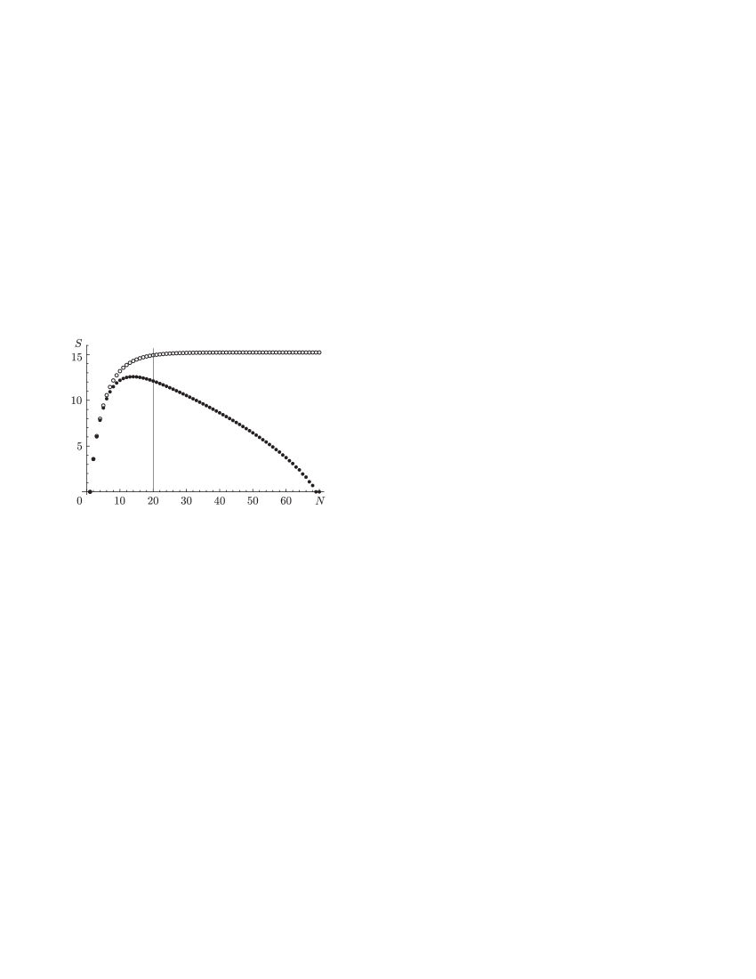
Figure 3: The dependence of the entropy $S$ on $N$ for $M=70$. The upper curve is obtained when zero summands are allowed, the lower one, when they are not. The vertical line indicates the value $N=N_{c}$ calculated according to formula (23). The exact value of the first point of the phase transition is the maximum of the lower curve.

The point of maximum of the lower curve in Fig. 3 for number theory is determined precisely. This is the value $N_{\max}$ for which the number $p_{N}(M)$ attains its maximum.

Now let us return to thermodynamics.

6 The Notion of Generalized Ideal Gas

We pass to the definition of the new classical ideal gas.

Note that in the description of the behavior of multi-particle systems it is possible that the initial conditions involve interactions. Consider the following analogy. There is a battery of canons. The gunners position the canons and interact with each other in the process. At some moment the command “Fire!” is heard (it means “all interactions (all conversations) must stop”). At the initial situation interactions took place, but once the canon balls are fired, they fly without interacting with each other. However elastic collisions between the balls are possible.

This model can be regarded as a model of ideal gas in the traditional understanding only if the initial data is given at time “minus infinity”.

A generalized classical ideal gas is a classical multi-particle system, where interactions cannot occur only inside certain open regions of the diagram, although at the initial moment of time or on the boundary of a region interactions between particles are allowed. In the region itself, only elastic collisions between particles are possible.

Why is it important to specify the open regions where no interaction (more precisely, no attraction) occurs? Obviously, if one must rapidly mix ball bearings of different sizes, it is easier to do this if the balls are not magnetized. The solution of this problem has several practical applications. Thus the speed with which two gases mix influences the driving force of jet engines: the higher the speed, the higher the driving force. If there is no attraction between molecules of a mixture of gases moving in a pipeline, the probability of the appearance of liquid bottlenecks is considerably less.

Thus the parameters of the Van-der-Waals gas coincide closely enough with the parameters of the new (generalized) gas in the following open regions of the parameters: 1) the region from the critical isotherm ($T_{r}=1$) to the critical isochore ($\rho=\rho_{c}$); 2) the region outside the gas spinodal; 3) the region of hard liquid (below the Temperley temperature, see Section 7).

7 Comparison of the Generalized Ideal Gas with the Van-der-Waals model

The main practical results that follow from the author’s theory are related to metastable states. In that sense, the main notion of the thermodynamics described here is not the binodal: the curve on the diagram that indicates the stable phase transition “vapor-to-liquid” (the gas binodal) and the phase transition “liquid-to-vapor” (the liquid binodal ). The main notion is the spinodal – the curve on the diagram that delimits the regions of stable and metastable states (a more precise definition of the spinodal was given above). It is practically impossible to reach values of the thermodynamical parameters on the spinodal experimentally, because that requires “infinite time”.

From relations (8)–(9) as $K\to\infty$ we obtain the following equations:

$$P_{r}=\frac{\Lambda(\gamma)T_{r}^{2+\gamma}\operatorname{Li}_{2+\gamma}(a)}{\zeta(2+\gamma_{c})},\qquad a=e^{\mu/T_{r}},\qquad\Lambda(\gamma)=\Lambda(\gamma,\infty)=\lim_{K\to\infty}\Lambda(\gamma,K),$$ (29)

$$\rho=\frac{\Lambda(\gamma)T_{r}^{1+\gamma}\operatorname{Li}_{1+\gamma}(a)}{\zeta(2+\gamma_{c})}.$$ (30)

For $a=1$, we obtain the spinodal defined above. This fact was proved by the author in [34].

The constants $\Lambda$ and $\gamma$ can be found for $a=1$ ($\mu=0$) from the coincidence of the values of $P_{r}$ and $\rho$ from (29) and (30) with the values of $P_{\text{sp}}$ and $\rho_{\text{sp}}$ on the Van-der-Waals spinodal.

In Figures 4 and 5, the isotherms of the Van-der-Waals model are compared with those of the author’s model on Hougen–Watson diagrams.

Figure 4: On this diagram the pressure is $P=P_{r}$. Coincidence of the Van-der-Waals isotherms (solid lines) with the isotherms from the author’s model (dashed lines). The following isotherms are shown $T_{r}=0.1$, $T_{r}=0.2$, $T_{r}=0.3$, $T_{r}=0.4$, $T_{r}=0.5$, $T_{r}=0.6$, $T_{r}=0.7$, $T_{r}=0.8$, $T_{r}=0.9$, $T_{r}=1$. The value of $\gamma=\gamma(T_{r})$ in equations (29)–(30) is determined from the relations on the Van-der-Waals spinodal $Z=Z_{sp}$, $P=P_{sp}$ for $a=1$.

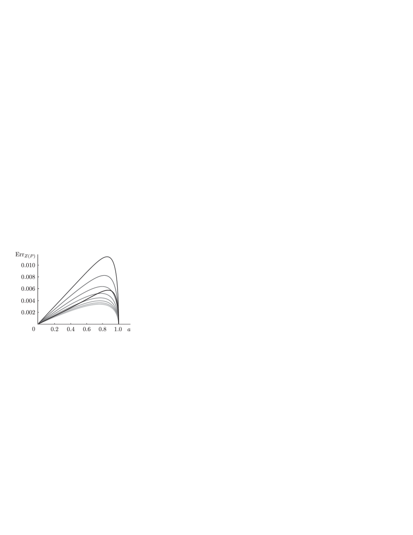
Figure 5: Discrepancy between the isotherms of the Van-der-Waals model and the isotherms obtained from the new distribution; $a=e^{\mu/T_{r}}$ is the activity, $T_{r}$ is the reduced temperature. The maximal discrepancy is $\sim 0.01$ for $T_{r}=0.9$ (the effect of $K\neq\infty$ is substantial).

In Figure 5, it is shown how the isotherms of the ideal gas (in the new sense) obtained from  (29)–(30), differ from the isotherms of the Van-der-Waals model. The figure shows that the isotherms practically coincide except at points near critical values. In regions with less than critical parameter values, the coincidence is up to 0.006%, while at points near critical values the error is of the order of 0.01%. Note the important point $0.9T_{c}$. At that point, the maximal discrepancy between the isotherms is observed. It is of the order of $\sim 0.01$.

For isotherms corresponding to temperatures less than the Temperley temperature (“cluster-free liquids”), we obtain a very precise coincidence between the isotherms constructed according to the distribution (29)–(30) and the isotherms coming from the Van-der-Waals model. The temperature $T_{\text{Temperly}}$ specifies a boundary above which the number $K$ (maximal occupation number) becomes infinite.

8 Analytical number theory and the energy of transition of the Bose gas to the Fermi gas

Niels Bohr [18] notes an important relationship between the number theory and the entropy, which arises in his concept of the nucleus. After that paper, several physicists, especially Hindu physicists [22]–[24], studied this problem and calculated the entropy for the Bose–Einstein gas and the entropy corresponding to the Ramanujan formula. These studies have been carried out up to now.

We show that, in the two-dimensional case, the formulas that were written for the Bose–Einstein distribution in the book [5] coincide with the formulas of analytical number theory.

Indeed, assume that there is a decomposition

$$M=a_{1}+\cdots+a_{N}$$

of a number $M$ into $N$ terms. By $N_{j}$ we denote the number of terms exactly equal to the number $j$ in the right-hand side of this decomposition.

Then the total number of terms is $\sum_{j}N_{j}$, and this number is equal to $N$, because we known that there is $N$ terms at all. Further, the sum of terms equal to $j$ is equal to $jN_{j}$, because there are $N_{j}$ of them and the sum of all terms is then obtained by summing these expressions over $j$, i.e., $\sum_{j}jN_{j}$, and it is equal to $M$. Namely,

$$\sum_{i=1}^{\infty}N_{i}=N,\qquad\sum_{i=1}^{\infty}iN_{i}=M.$$ (31)

Let us consider an example of the well-known Erdős theorem in the number theory, i.e., the solution of ancient problem called “partitio numerorum” in Latin. This problem deals with an integer $M$ which is decomposed into $N$ terms, for example, $M=5$, $N=2$:

$$5=1+4=2+3=0+5,$$

which gives three versions $\mathcal{M}$ of the solution of this problem: $\mathcal{M}=3$.

If $M=10^{23}$, $N=1$, then there is only one version: $\mathcal{M}=1$. If $M=10^{23}$ and $N=10^{23}$, then there is also only one version, i.e., the sum of units, $\mathcal{M}=1$.

Obviously, for a fixed $M$, there exists a number $\tilde{N}$ for which the number of decomposition versions $\mathcal{M}$ is maximal (in general, this number is not unique). The number $\log_{2}\mathcal{M}$ is called the Hartley entropy. At the point where it attains its maximum, the entropy is also maximal. The chemical potential equal to zero corresponds to this point. The Erdős formula determines the maximal number of solutions of the decomposition function $\tilde{N}$ and has the form

$$\tilde{N}=\beta^{-1}M^{1/2}\log M+\alpha M^{1/2}+o(M^{1/2}),\qquad\beta=\pi\sqrt{2/3},$$ (32)

where the coefficient $\alpha$ is determined by the formula $\beta/2=e^{-\alpha\beta/2}$.

Erdős obtained his result only up to $o(\sqrt{M})$ because of the nonuniqueness of the above-mentioned maximum and the ambiguity of the number of these maxima

Remark 2.

The classical number theory deals with the space $\mathbb{Z}$ of integers. Generalizations to the space $\mathbb{R}^{+}$ were obtained in the works which were surveyed in detail by A.G. Postnikov in the book [45]. This approach agrees well with the concept of statistical physics, where some of the variables belong to $\mathbb{R}$, and hence the integers such as the number of particles $N$ and the parastatistical number $k$ (restricting the number of particles at one energy level), together with various numbers belonging to the set $\mathbb{R}$, loose their meaning of integer numbers.

Erdős considered the case where the number $N$ is fixed. We shall consider the sum of all decomposition versions less than or equal to $N$. Obviously, in this case, the maximal entropy is also between $N$ and zero. The formula is of the same order as in the Erdős, but the answer is significantly different.

Let us consider this question in more detail.

The following formulas hold for the Bose–Einstein distribution in the case of $D$ degrees of freedom [5], [26]:

$$E=\Phi T(\gamma+1)\operatorname{Li}_{2+\gamma}(a),\quad N=\Phi\operatorname{Li}_{1+\gamma}(a).$$ (33)

Here and below, $\gamma=D/2-1$, $T$ is the temperature, $a=e^{\mu/T}$ is the activity, $\mu$ is the chemical potential.

The following formulas hold for the Fermi–Dirac distribution:

$$E=-\Phi T(\gamma+1)\operatorname{Li}_{2+\gamma}(-a),\ N=-\Phi\operatorname{Li}_{1+\gamma}(-a).$$ (34)

We see that formulas (33) and (34) differ in sign, and hence the activity $a$ passes through the point $a=0$.

9 Boson–Ferminon Transition in Mesoscopy

Our goal is to determine the energy of transition of Bose particles to Fermi particles. For this, it suffices to study the transition of (33) into (34) through the point $a=0$. If we want to extend the interval of the jump from the Bose distribution to the Fermi distribution, then it is necessary to use the parastatistics or the Gentile statistics [10].

In the case of parastatistics, we have relations, where the first term in parentheses gives the distribution for Bose particles, and the second term, the parastatistical correction:

$$E={\Phi}T({\gamma+1})(\operatorname{Li}_{2+\gamma}(a)-\frac{1}{(k+1)^{\gamma+1}}\operatorname{Li}_{2+\gamma}(a^{k+1})),$$ (35)

$$N={\Phi}(\operatorname{Li}_{1+\gamma}(a)-\frac{1}{(k+1)^{\gamma}}\operatorname{Li}_{1+\gamma}(a^{k+1})).$$ (36)

We let $N_{i}$ denote the number of particles at the $i$th energy level. In the case of parastatistics, there can be at most $k$ particles at each energy level. By the usual definitions, the Fermi case is realized for $k=1$, and the Bose case, for $k=\infty$. But by formulas (31), it is obvious that $N_{i}\leq N$ for the Bose system. Therefore, $k\leq N$ for the Bose system. This implies that the maximal value of $k$ is equal to $N$, but not to infinity. This logical conclusion significantly changes the formulas. In particular, there arise new equations for $N=k$:

$$E={\Phi}T({\gamma+1})(\operatorname{Li}_{2+\gamma}(a)-\frac{1}{(N+1)^{\gamma+1}}\operatorname{Li}_{2+\gamma}(a^{N+1})),$$ (37)

$$N={\Phi}(\operatorname{Li}_{1+\gamma}(a)-\frac{1}{(N+1)^{\gamma}}\operatorname{Li}_{1+\gamma}(a^{N+1})).$$ (38)

The maximal number of particles at the energy level $N_{c}$ in the system occurs at the caustic point $a=1$.

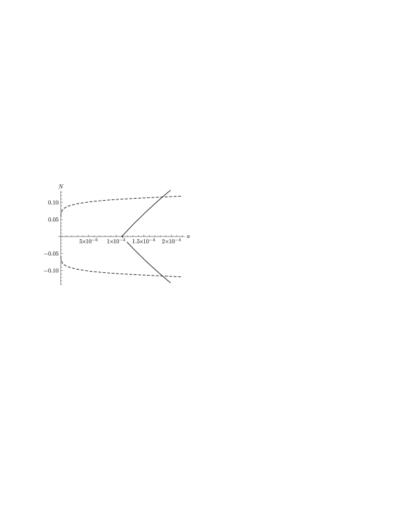
Figure 6: Graph of the dependence $N(a)$ for $W=1000$, $W=V(\lambda^{2}T)^{\gamma+1}$, where $\lambda$ is a parameter depending on the mass and $\gamma=0$. The dotted curve corresponds to $N=-1/\log(a)$. The solid line corresponds to $N=0$.

9.1 Case of small N

As was pointed out above, the author obtained a self-consistent equation (38), where $N$ is an unknown quantity. We are interested in the point at which the number of Bose particles $N$ is equal to 0, i.e., the point at which the Bose particles disappear. Figure 6 illustrates an example of this point. We stress that the value of the activity $a$ does not vanish at this point, but significantly depends on the function $\Phi$ and the parameter $\gamma$.

Let us consider the mesoscopic case. We expand the right-hand side of Eq. (38) in a power series in $N\to 0$. Using the identity for the polylogarithm

$$z\frac{\partial\operatorname{Li}_{s}(z)}{\partial z}=\operatorname{Li}_{s-1}(z),$$ (39)

we obtain the following expansion in the Taylor series in a small $N$:

$$\frac{1}{(N+1)^{\gamma}}=1-\gamma N+\frac{1}{2}\left(\gamma^{2}+\gamma\right)N^{2}+O\big{(}N^{3}\log^{3}(a)\big{)},$$

$$\operatorname{Li}_{1+\gamma}(a^{N+1})=\operatorname{Li}_{\gamma+1}(a)+N\log(a)\operatorname{Li}_{\gamma}(a)+\frac{1}{2}N^{2}\log^{2}(a)\operatorname{Li}_{\gamma-1}(a)+O\big{(}N^{3}\log^{3}(a)\big{)}.$$

This implies

$$\begin{split}&\operatorname{Li}_{1+\gamma}(a)-\frac{1}{(N+1)^{\gamma}}\operatorname{Li}_{1+\gamma}(a^{N+1})=N(\gamma\operatorname{Li}_{\gamma+1}(a)-\log(a)\operatorname{Li}_{\gamma}(a))\\ &+\frac{1}{2}N^{2}\left(\gamma^{2}(-\operatorname{Li}_{\gamma+1}(a))-\gamma\operatorname{Li}_{\gamma+1}(a)-\log^{2}(a)\operatorname{Li}_{\gamma-1}(a)+2\gamma\log(a)\operatorname{Li}_{\gamma}(a)\right)+O\big{(}N^{3}\log^{3}(a)\big{)}.\end{split}$$ (40)

Then the expansion of the number $N$ becomes (up to $o(N^{2}\log^{2}(a))$):

$$\begin{split}&\frac{N}{V}=(\lambda^{2}T)^{\gamma+1}[N(\gamma\operatorname{Li}_{\gamma+1}(a)-\log(a)\operatorname{Li}_{\gamma}(a))\\ &+\frac{1}{2}N^{2}\left(\gamma^{2}(-\operatorname{Li}_{\gamma+1}(a))-\gamma\operatorname{Li}_{\gamma+1}(a)-\log^{2}(a)\operatorname{Li}_{\gamma-1}(a)+2\gamma\log(a)\operatorname{Li}_{\gamma}(a)\right)].\end{split}$$ (41)

Dividing Eq. (41) by $N$, we obtain

$$\begin{split}&\frac{1}{V}=(\lambda^{2}T)^{\gamma+1}[(\gamma\operatorname{Li}_{\gamma+1}(a)-\log(a)\operatorname{Li}_{\gamma}(a))\\ &+\frac{1}{2}N\left(-(\gamma^{2}+\gamma)\operatorname{Li}_{\gamma+1}(a)-\log^{2}(a)\operatorname{Li}_{\gamma-1}(a)+2\gamma\log(a)\operatorname{Li}_{\gamma}(a)\right)].\end{split}$$ (42)

This implies

$$\begin{split}&-1+V(\lambda^{2}T)^{\gamma+1}(\gamma\operatorname{Li}_{\gamma+1}(a)-\log(a)\operatorname{Li}_{\gamma}(a))\\ &+\frac{V(\lambda^{2}T)^{1+\gamma}}{2}N\left(-(\gamma^{2}+\gamma)\operatorname{Li}_{\gamma+1}(a)-\log^{2}(a)\operatorname{Li}_{\gamma-1}(a)+2\gamma\log(a)\operatorname{Li}_{\gamma}(a)\right)=0.\end{split}$$ (43)

To pass from the case $k=0$ to the case $k=\infty$, it is necessary to use the natural series of numbers. We will consider this transition below. We assume that $k=N$ in an infinitely small neighborhood of the resonance $[N]$, where $[N]$ is the integer part of the number $N$. The set of points infinitely close to the number $[N]$ is called a monad in the nonstandard analysis or the Leibnitz differential (see [52]–[53], and also see [54]–[55]). We let $x$ denote the difference $N-[N]$, i.e., $N-[N]=x>0$. We see the expansion in a power series in $x$ up to $O(x^{2})$, which implies $N\sim|N|$.

The self-consistent relation for $x$ near the resonance points $[N]$ has the form

$$[N]+x={(T\lambda)^{\gamma+1}V}(\operatorname{Li}_{1+\gamma}(a)-\frac{1}{([N]+x+1)^{\gamma}}\operatorname{Li}_{1+\gamma}(a^{[N]+x+1})).$$ (44)

The following thermodynamic formula is known for the pressure $P$:

$$P=T{(T\lambda)^{\gamma+1}}(\operatorname{Li}_{2+\gamma}(a)-\frac{1}{([N]+x+1)^{\gamma+1}}\operatorname{Li}_{2+\gamma}(a^{[N]+x+1})).$$ (45)

In the Gentile statistics, each $\Phi$ is associated with its own value of activity $a$ at which the number of particles is $N=0$. In this case, the Bose particles disappear. They split into Fermi particles and the Bose statistics turns into the Fermi statistics. We denote such a value by $a_{0}$.

Let us consider the behavior of the system in the case of distinct values of $k$.

9.2 Expansion near $k=0$

As was shown above, the number of particles at the energy level cannot exceed $N$. We can expand the right-hand side of Eq. (44) in small $N$ neglecting the terms $O((N-k)^{2})$ as

$$\begin{split}&N=\Phi N(\gamma\operatorname{Li}_{\gamma+1}(a)-\log(a)\operatorname{Li}_{\gamma}(a))\\ &+\Phi\frac{1}{2}N^{2}\left(\log^{2}(a)(-\text{Li}_{\gamma-1}(a))-\gamma((\gamma+1)\operatorname{Li}_{\gamma+1}(a)-2\log(a)\operatorname{Li}_{\gamma}(a))\right).\end{split}$$ (46)

Passing to the limit in (46) as $N\to 0$, we obtain the equation for $a$ for which $N=0$:

$$\gamma\operatorname{Li}_{\gamma+1}(a_{0})-\log(a_{0})\operatorname{Li}_{\gamma}(a_{0})-\Phi^{-1}=0.$$ (47)

For a sufficiently large $\Phi$, this equation has a unique solution which we denote by $a_{0}$.

In this case, the error is the difference between the noninteger solution $N$ for $a>a_{0}$ and the integer $N=0$ for $a=a_{0}$, i.e., $x=N-0=N$.

9.3 Expansion near $k=1$

Let $N=1+x$, where $x$ is small. The expansion of the right-hand side of (44) for small $x$ leads to the equation for $x$:

$$1+x=\Phi[\text{Li}_{\gamma+1}(a)-2^{-\gamma}\operatorname{Li}_{\gamma+1}\left(a^{2}\right)-2^{-\gamma-1}x\left(2\log(a)\operatorname{Li}_{\gamma}\left(a^{2}\right)-\gamma\operatorname{Li}_{\gamma+1}\left(a^{2}\right)\right)+O(x^{2})].$$ (48)

The equation for $a$ at which $x=0$ or $N=1$ has the form

$$-\Phi\operatorname{Li}_{\gamma+1}\left(a^{2}\right)+2^{\gamma}\Phi\operatorname{Li}_{\gamma+1}(a)-2^{\gamma}=0.$$ (49)

This equation has a unique solution which we denote by $a_{1}$ following the notation introduced above.

In this case, the error is the difference between the solution of the equation for noninteger $N$ and $a>a_{1}$ and the solution of the equation for integer $N=1$ and $a=a_{1}$, i.e., $x=N-1$.

The pressure expansion (45) for small $x$ up to the first order inclusively has the form

$$P=\frac{\Phi T}{V}[\left(\text{Li}_{\gamma+2}(a)-2^{-\gamma-1}\operatorname{Li}_{\gamma+2}\left(a^{2}\right)\right)+x\left(2^{-\gamma-2}(\gamma+1)\operatorname{Li}_{\gamma+2}\left(a^{2}\right)-2^{-\gamma-1}\log(a)\operatorname{Li}_{\gamma+1}\left(a^{2}\right)\right)].$$ (50)

9.4 Expansion near an arbitrary positive integer $k=i$.

After similar calculations, one can obtain the asymptotic formulas for the error in determining $N$ and the pressures $P$ near $k=2$:

$$x=N-2,$$ (51)

$$P=\frac{\Phi T}{V}[\left(\text{Li}_{\gamma+2}(a)-3^{-\gamma-1}\operatorname{Li}_{\gamma+2}\left(a^{3}\right)\right)-3^{-\gamma-2}x\left(-\gamma\operatorname{Li}_{\gamma+2}\left(a^{3}\right)-\text{Li}_{\gamma+2}\left(a^{3}\right)+3\log(a)\operatorname{Li}_{\gamma+1}\left(a^{3}\right)\right)].$$ (52)

For an arbitrary positive integer $i$, we have the relations

$$x=N-i,$$ (53)

$$\begin{split}&P=\frac{\Phi T}{V}[\left(\text{Li}_{\gamma+2}(a)-(i+1)^{-\gamma-1}\operatorname{Li}_{\gamma+2}\left(a^{i+1}\right)\right)\\ &-x(i+1)^{-\gamma-2}\left(-(\gamma+1)\operatorname{Li}_{\gamma+2}\left(a^{i+1}\right)+(i+1)\log(a)\operatorname{Li}_{\gamma+1}\left(a^{i+1}\right)\right)].\\ \end{split}$$ (54)

The equation for $a_{i}$ at which $N=i$ has the form

$$-\Phi\operatorname{Li}_{\gamma+1}\left(a^{i+1}\right)+(i+1)^{\gamma}\Phi\operatorname{Li}_{\gamma+1}(a)-i\ (i+1)^{\gamma}=0.$$ (55)

The solutions of Eq. (55) are shown in Figs. 7, 8, and 9.

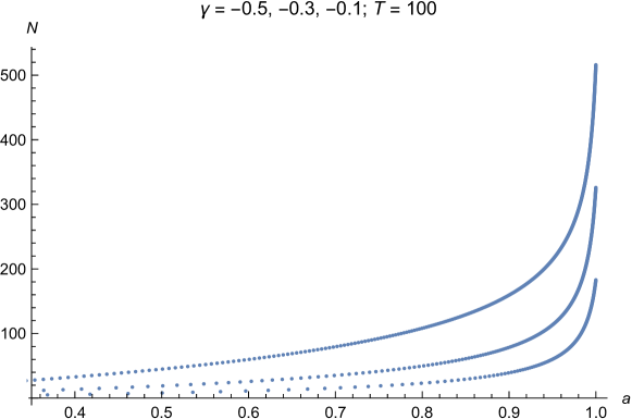
Figure 7: Dependence of the number of particles $N$ on $a$ for a given temperature $T=100$ which is the result of numerical solution of Eq. (55). Here $\gamma=-0.5,-0.3,-0.1$ counting upwards from below. For $\gamma=-0.5$, the maximum $N=183$ is attained at $a=0.999906$. For $\gamma=-0.3$, the maximum $N=326$ is attained at $a=0.999954$. For $\gamma=-0.1$, the maximum $N=516$ is attained at $a=0.999985$.

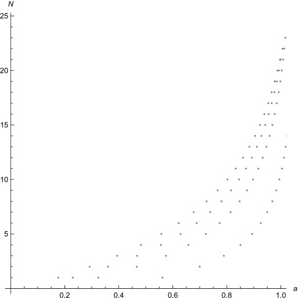
Figure 8: Dependence of the number of particles $N$ on $a$ for a given energy $M=70$ which is the result of numerical solution of the system of Eqs. (44), (45). Here $\gamma=-0.7,-0.5,-0.3,-0.1$ counting upwards from below. The values of maximal $a_{i}$ are given in (57).

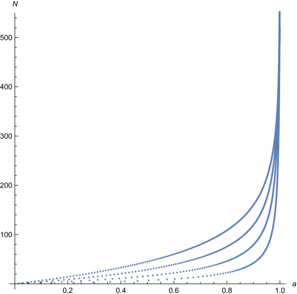
Figure 9: Dependence of the number of particles $N$ on $a$ for a given energy $M=10000$ which is the result of numerical solution of the system of Eqs. (44), (45). Here $\gamma=-0.7,-0.5,-0.3,-0.1$ counting upwards from below. The values of maximal $a_{i}$ are given in (58).

Note that, for given values of the parameters $\Phi$ and $\gamma$, Eq. (55) has the maximal solution $a_{i}=a_{max}<1$ corresponding to the maximal $i=i_{max}$.

As was said above, $M$ is the total energy of all particles. Putting $\mu=0$, neglecting the negative term in formula (45) as $N\to\infty$, and using the well-known thermodynamical relation $M=(\gamma+1)PV$, we express the temperature in terms of the parameters $M,\gamma,\lambda,V$ as follows:

$$T(M,\gamma,\lambda,V)=\left(\frac{M}{(\gamma+1)V\lambda^{1+\gamma}\zeta(2+\gamma)}\right)^{\frac{1}{\gamma+2}}.$$ (56)

Thus, the temperature is determined on the spinodal.

In (57) and (58), we present the corresponding values $a_{max}$, $i_{max}$ for $M=70$ and $M=10000$.

$$M=70:\left(\begin{array}[]{ccc}\gamma&i_{max}&a_{max}\\ -0.1&21&0.995525\\ -0.3&22&0.991582\\ -0.5&23&0.997874\\ -0.7&17&0.994192\\ \end{array}\right)$$ (57)

$$M=10000:\left(\begin{array}[]{ccc}\gamma&i_{max}&a_{max}\\ -0.1&519&0.99998\\ -0.3&631&0.999991\\ -0.5&784&0.999964\\ -0.7&817&0.999999\\ \end{array}\right)$$ (58)

9.5 Jump of the specific energy

Now we consider the situation where only the parameter $a$ varies at a fixed temperature, namely, for the Bose case, it varies from $a_{max}$ to $a_{0}$, and for the Fermi case, from $0$ to infinity.

If we consider only traditional formulas for the Bose gas which correspond to the case where infinitely many particles can be located at each energy level, then the negative term in the integrand in formulas (44) and (45) is absent. In this case, the transition of a boson particle to a fermion particle is accompanied by the change of the sign of the activity $a$ in all formulas, where the polylogarithm function is contained. Indeed, for the Bose–Einstein distribution, we have

$$\operatorname{Li}_{\gamma+1}(a)=\frac{1}{\Gamma{(\gamma+1)}}\int_{0}^{\infty}{\frac{\xi^{\gamma}d\xi}{e^{\xi}/a-1}},$$ (59)

and for the Fermi–Dirac distribution, we have

$$-\operatorname{Li}_{\gamma+1}(-a)=\frac{1}{\Gamma{(\gamma+1)}}\int_{0}^{\infty}{\frac{\xi^{\gamma}d\xi}{e^{\xi}/a+1}}.$$ (60)

Thus, we can assume that the activity is equal to $-a$ and negative for the Fermi case, and it is equal to $a$ and remains positive for the Bose case.

If the activity $a$ changes sign, this means that it necessarily passes through the transition point $a=0$ at which both the pressure and the number of particles are equal to zero. To avoid the change of sign of the polylogarithm function, we assume that the values of the energy $M$ and the pressure $P$ and hence the number of particles $N$ of the Bose gas are negative.

But in contrast to Eqs. (44) and (45), the above obtained equations determine the transition point not for $a=0$ but for $a=a_{0}>0$. Precisely at this point, as will be shown below, the compressibility factor $Z=\frac{PV}{NT}$ and hence the specific energy experience a jump.

The jump $Z$ is visually illustrated in Fig. 10.

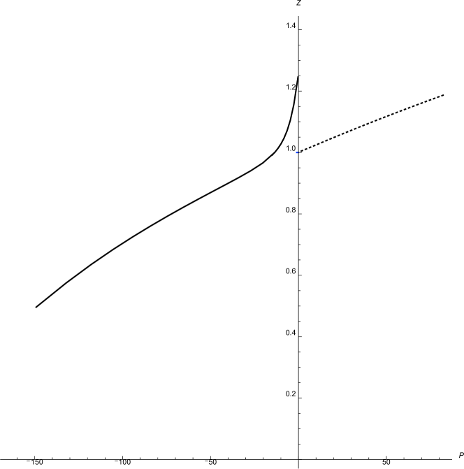
Figure 10: Dependence of the compressibility factor $Z$ on $P$ at a given temperature $T=10$. The solid curve on the left corresponds to the Bose case, the dashed curve on the right, to the Fermi case. The jump of the compressibility factor is equal to $\Delta Z=-0.25$.

Starting from the value of the compressibility factor $Z=\frac{PV}{NT}$, we obtain the expression for the specific energy: $E_{sp}=\frac{E}{N}=Z(\gamma+1)T>0$. The limit of the function $Z$ as $P\to+0$ from the right, which corresponds to the Fermion branch, is equal to $1$. The limit of $Z$ as $P\to-0$ from the left, as was shown in [56], is equal to $Z_{0}(M,\gamma,\lambda,V)$, where

$$Z_{0}(M,\gamma,\lambda,V)=\lambda^{\gamma+1}V[T(M,\gamma,\lambda,V)]^{1+\gamma}(\gamma\text{Li}_{\gamma+2}(a_{0})+\text{Li}_{\gamma+2}(a_{0})-\log(a_{0})\text{Li}_{\gamma+1}(a_{0}))>1.$$ (61)

In such a transition, the compressibility factor has a jump by the value $\Delta Z=Z_{Fermi}-Z_{Bose}=1-Z_{0}<0$. This corresponds to the jump of the specific energy equal to $\Delta E_{sp}=T(\gamma+1)(Z_{Fermi}-Z_{Bose})=T(\gamma+1)(1+Z_{0})<0$.

Table 1 presents the values of $Z_{0}$ for different $\gamma$ for $M=200$ under the condition $\lambda^{\gamma+1}V=1$.

Table 1:

$\gamma$	-0.7	-0.6	-0.5	-0.4	-0.3	0
$Z_{0}$	1.54	1.44	1.38	1.34	1.31	1.25

Figure 11: Dependence of $Z_{0}(M,\gamma,\lambda,V)$ on $\gamma$ for a given energy $M=200$, constructed by formula (61).

The dependence of $Z_{0}(M,\gamma,\lambda,V)$ on $\gamma$ for a given energy $M=200$ is shown in Fig. 11, where the behavior of $Z_{0}$ is shown for the continuously varying value $\gamma\in(-1,0]$.

10 Transition of the Helium-6 boson to the Helium-5 fermion

Following the author’s concept related to the abstract analytical number theory [45], one can mathematically calculate the transition of Bose particles to Fermi particles, at least in the two-dimensional case. Based on this concept, the boson branch of the decomposition of the number $M$ into terms (with possible repetition of terms) turns into the fermion branch of the decomposition (without repeated terms). It follows from the continuity of such a transition that there exists a point of transition from the boson branch into the fermion branch according to the number of terms $N$.

The specific volume $V$ (the area in the two-dimensional case) was determined in the number theory in [46] as $N=V\operatorname{Li}_{1}(a)$ for the distribution of the Bose gas. Here $N/V$ is the density. For the volume $V$, the energy can be written as $E=V\operatorname{Li}_{2}(a)$.

When the activity $a$ changes the sign, the boson branch (with repetition of terms in the decomposition of the number) in the number theory turns into the fermion branch (without repetition of the terms in the decomposition). One succeeds in passing from the number theory to the case of small dimension, i.e., to any number of degrees of freedom greater or smaller than 2. In this case, on succeeds in calculating the coefficient of $1/\log a$, which permits determining the value of the energy required for the Bose gas to go over into the Fermi gas (for example, Helium-4 into Helium-3) for a given volume and a given temperature.

10.1 Quantization of activity and energy of Gödel, Maltsev and Ershov numbering. Calculation of the hidden parameter for the microscopy

In this and other works, the author considered the “hidden parameter” $t_{\mathrm{meas}}$, which is not hidden in the sense of the Einstein–Podolsky–Rosen paradox (EPR). The parameter introduced by the author is quite natural and open. In the assertion on the identity of particles in the works of Landau and Lifshits [7] which has been many times cited by the author in his papers, this parameter is veiled as the “time moment” at which the numeration of particles is attained. This citation states the following: “one can imagine that the particles contained in a given physical system are “renumbered” at a certain time moment” (p. 252). The time required to numerate the particles is precisely the additional parameter introduced by the author in [27], [57]–[58] and which is discussed in the present paper. This time depends on the algorithm used to numerate the particles. In turn, the time of implementation of the algorithm depends on the calculating person and his device. Thus, this parameter is not hidden but is a somewhat veiled. It can be determined exactly only under a lot of additional conditions.

In the paragraph of the book [7] cited above, Landau and Lifshits also speak about other time moments, namely, if “one further watches the motion of each of the particles in its trajectory, then the particles can be identified at any time moment” (italics added by VM).

The time moments form a discrete set of points. It the intervals between these points are much less than the veiled parameter, then the observer sees the classical picture of the neutron (wave packet) revolution around the Helium-4 nucleus independently of the life time of the Helium-5 fermion.

We consider a gas, i.e., a sufficiently many particles, each of which is a boson. If we consider specific characteristics of the gas (specific energy, specific volume, etc.), then we can assume that these specific quantities are related to the microscopy, i.e., to the situation of a single nucleus with several nucleons.

Assume that the hidden parameter $t_{\mathrm{meas}}$ (i.e., the time given to the experimenter for observation) is of the order of $10^{-11}$, and the life time of a boson is of the order of $10^{-13}$. Our assumption is not strict, but since the value of time of the order of $10^{-11}$ is much greater than the value of the order of $10^{-13}$, and hence much greater than the time during which the experimenter observed 20 boson revolutions around the nucleus, we can assume that this value of time is approximately equal to the hidden parameter in the microscopy in the sense explained above. If we have one nucleus and each nucleon is a boson, then for the bosons in this approximation (in terms of approximate specific energies), we can calculate the sum of specific energies for all bosons. This total energy coincides with the energy of microparticles, i.e. for all nucleons in the order sufficient for us.

Indeed, we are interested not in the energy but in the hidden parameter $t_{\text{meas}}$. With regard to the above, we can state the hidden parameter is revealed with a sufficient accuracy, i.e., with a logarithmic accuracy.

In the present paper, we propose a method for determining the energy of fermions and bosons in the case of a gas, i.e., in the case where there are very many particles. For the specific energy, we can add the specific values of separate particles and obtain the microscopic sum of energies of separate nucleons. Since the hidden parameter is calculated approximately (with a logarithmic accuracy), we can justify the method proposed for calculations.

In [18], it is similarly proposed to sum the microscopic energies of particles to calculate the binding energy of the whole nucleus. This permits calculating the value of the hidden parameter.

Let us consider the specific energy of a gas consisting of particles obeying the Bose–Einstein statistics for $a=1$:

$$E_{spec}=T(\gamma+1)\frac{\zeta(2+\gamma)}{\zeta(1+\gamma)}.$$ (62)

This energy corresponds to the macroscopy, while the specific binding energy of the nucleus $\epsilon$, i.e., the energy per 1 nucleon, corresponds to the microscopy. The equality of these energies permits calculating the parameter $\beta=\frac{1}{T}$:

$$\beta=(\gamma+1)\frac{\zeta(2+\gamma)}{\epsilon\zeta(1+\gamma)}.$$ (63)

The time $t_{0}$ equal to the interval between the moments of measurement can be calculated by the formula

$$t_{0}=\beta\hbar=(\gamma+1)\hbar\frac{\zeta(2+\gamma)}{\epsilon\zeta(1+\gamma)},$$ (64)

where $\hbar$ is the Plank constant.

For Helium-5, the specific binding energy is equal to $5.481$ MeV, the life time of the nucleus is $1.01\times 10^{-21}$ s, and the time $t_{0}=5.2\times 10^{-22}$ s for $\gamma=3.5$. For Helium-6, the specific binding energy is equal to $4.878$ MeV, the life time of the nucleus is $1.16$ d, and the time $t_{0}=5.9\times 10^{-22}$ s for $\gamma=3.5$.

The dependence $t_{0}(\gamma)$ is depicted in Fig. 12. In particular, for $\gamma=0.5$, the life time for Helium-5 is equal to $9.25\times 10^{-23}$ S, and for Helimu-6, to $1.04\times 10^{-22}$ s.

Figure 12: Dependence of the time $t_{0}(\gamma)$ given by formula (64). The upper curve corresponds to Helium-6, the lower, to Helium-5.

We assume that to distinguish one revolution of a neutron around the nucleus, the experimenter has to take at least 10 pictures in this time period. Thus, to distinguish 20 revolutions, it is necessary to take 200 during the time $200t_{0}$. In the case $\gamma=3.5$ for Helium-5, this time is equal to $t_{0}=1.05\times 10^{-19}$ s, which significantly exceeds the time given for the experiment, i.e., the value of the hidden parameter.

Thus if the life time of a particle is less that the time given for the experimental observation (i.e., less that the hidden parameter), then the experimenter can distinguish this particle from the others. But if the life time of a particle is greater than the observation time, then the the experimenter cannot distinguish the particles. But during the time given to him, he can observe some separate moments or stages of the particle life, for example, 20 revolutions of the particle around the nucleus. But these separate moments of the particle life do not allow him to distinguish this particle from the other particles, i.e. to identify it,

In other words, our concept is based on the following three times: the time given for the experiment (hidden parameter), the life time of a particle, and the real time of events in the life of a particle which is less than the time of its whole life and which is observed by the experimenter.

Since we distinguish the hidden parameter in the quantum mechanics and the hidden parameter in classical statistical physics, it is necessary, more precisely than usually in the physical literature, to separate the quantum quantities and the classical quantities which disappear as $\hbar\to 0$. For example, in the literature, the light polarization is related to the wave optics, despite the fact that, as is known, the polarization does not disappear as the frequency tends to infinity and hence remains in the geometric optics.

Similarly, the spin does not disappear in the classical limit $\hbar\to 0$ and is preserved in the classical transport equation [29], [59]. The hidden parameter for the spin is not related to the quantum hidden parameter $\Delta t=\hbar/\Delta E$.

The WKB method of transition from the quantum mechanics in classical mechanics leads to the following two classical equations: the Hamilton–Jacobi equation and the transport equation. Both of these equations describe the classical mechanics. The Hamilton–Jacobi equation contains a term which determines the interaction of particles in the Newton equation The interaction between the spin and the magnetic field is contained in the transport equation, and hence can be explained in classical mechanics. The question of how to describe the interaction between the terms in the transport equation if there is no interaction in the Hamilton–Jacobi equation was posed by Anosov and by the author at the beginning of the 1960s. At present, this problem is related to the Bell inequality and hence to the hidden parameters arising in this case [60]. The author agrees with Bohm in that the main difficulty in revealing the EPR paradox reduces to a problem related to the spin and polarization. But as follows from the above, this by no means does not concern the problem of the quantum hidden parameter considered in this section. The difficulty is in the problem of spin, and it reduces to the classical mechanics. Precisely in the same way, we can neglect the Newtonian attraction.

The experiment with rotation of a boson around the nucleus revealed the following. On the one hand, the experimenter allowed an increase in the hidden parameter to such an extent that the wave packet corresponding to the nucleon began to differ from its twin. This implies that the nucleon started to behave not as a quantum particle, which is located at a separate Bohr energy level, but as a classical particle, which rotates as the Rutherford electron.

This fact already shows that, even for small energies, the nucleon does behave according to the Bohr rule related to separate orbits. Does this mean that there is a WKB approximation? The transition to the classics was previously explained only by the WKB approximation. But the experiments allowed one to calculate the hidden parameter and confirmed the fact that the hidden parameter is large so that it permits observing the behavior of a nucleon separately from its twin behavior. By the hidden parameter law, the nucleon behaves like a wave packet independently of its twin, and hence it makes revolutions.

Thus, this well-known experimental fact can be explained by using the hidden parameter, which permits considering the classical mechanics and the quantum mechanics from the common point of view. This unifies the two sciences into a comprehensive whole and exactly shows when we must pass from the quantum theory to the classical theory without using the WKB method. This is a principally different method for such a transition as compared to the WKB method. In what follows, we show the converse; namely, the quantum problem, in turn, gives important results in classical theory of thermodynamics without the semiclassical transition.

References

- [1] Maslov V. P. Undistinguishing Statistics of Objectively Distinguishable Objects: Thermodynamics and Superfluidity of Classical Gas. Math. Notes 2013; 94 (5):722-813.
- [2] Maslov V. P. New Construction of Classical Thermodynamics and UD-Statistics. Russian J. Math. Phys. 2014; 21 (2):256-284.
- [3] Maslov V. P. Thermodynamics and Economics: Overview. Reference Module in Earth Systems and Environmental Sciences. Elsevier; 2014.
- [4] Dobrokhotov S. Yu., Karasev M. V., Kolokoltsov V. N., et al. Award of the State Prize of the Russian Federation in Science and Technology (2013) to Victor Maslov. Probability Theory and Applications 2014; 59 (2):2009–2013.
- [5] Landau L. D. and Lifshits E. M. Statistical Physics. Moscow: Nauka; 1964 [in Russian].
- [6] Kadomtsev B. B. Dynamics and Information. Moscow, Uspekhi Fizicheskikh Nauk; 1999 [in Russian].
- [7] Landau L. D. and Lifshits E. M. Quantum Mechanics: Non-Relativistic Theory, 2nd ed. Moscow:Nauka; 1964 [in Russian]; (translation of the 1st ed., Pergamon Press, London–Paris and Addison-Wesley Publishing Co., Inc., Reading, Mass.; 1958).
- [8] Maslov V. P. and Shvedov O. Yu. The Complex Germ Method in Many-Particle Problems and in Quantum Field Theory. Moscow: Editorial URSS; 2000 [in Russian].
- [9] V. P. Maslov, “Hidden variables in the theory of measuring,” Math. Notes 102 (6), (2017).
- [10] Dai W.-S., Xie M.Gentile statistics with a large maximum occupation number. Annals of Physics 2004 309:295–305.
- [11] Maslov V. P. The relationship between the Van-der-Waals model and the undistinguishing statistics of objectively distinguishable objects. The new parastatistics. Russian J. Math. Phys. 2014; 21 (1):99–111.
- [12] Vershik A. M. Statistical mechanics of combinatorial partitions, and their limit shapes,” Funktsional. Anal. i Prilozhen. 1996; 30 (2): 19–39 [Functional Anal. Appl. 1996; 30 (2):90–105].
- [13] Maslov V. P. Nazaikinskii V. E. On the rate of convergence to the Bose-Einstein distribution. Math. Notes 2016; 99 (1):95–109.
- [14] Maslov V. P. Case of less than two degrees of freedom, negative pressure, and the Fermi–Dirac distribution for a hard liquid,” Math. Notes 2015; 98 (1):138–157.
-
[15]
V. P. Maslov, ‘
‘New Insight into the Partition Theory of Integers
Related to Problems of Thermodynamics and Mesoscopic Physics,” Math. Notes 102 (2) 234– 251 (2017). - [16] Albert Einstein—Hedwig and Max Born, Briefwechsel 1916–1955 (Nympherburger Verlagshandlung, München, 1969).
- [17] J. D. Cockcroft and E. T. Walton, ”Experiments with high velocity positive ions. II. The disintegration of elements by high velocity protons,” Proc. Royal Soc. A 137, 229–242 (1932).
- [18] N. Bohr and F. Kalckar “On the transformation of atomic nuclei due to collisions with material particles,” Uspekhi Fiz. Nauk 20 (3), 317–340 (1938).
- [19] N. Bohr and J. A. Wheeler, “The mechanism of nuclear fission,” Phys. Rev. 56, 426n450 (1939).
- [20] E. M. Lifshits and L. P. Pitayevskii, Theoretical Physics, Vol. X: Physical Kinetics (Fizmatlit, Moscow, 2007) [in Russian].
- [21] E. M. Lifshits and L. P. Pitaevskii, Statistical Physics, Vol. X: Part 2: Theory of Condensed State (Nauka, Moscow, 1978; Pergamon, Oxford, 1980).
- [22] F. C. Auluck and D. S. Kothari, “Statistical mechanics and the partitions of numbers,” Math. Proc. Cambridge Philos. Soc. 42, 272–277 (1946).
- [23] B. K. Agarwala and F. C. Auluck, “Statistical mechanics and the partitions into non-integral powers of integers,” Math. Proc. Cambridge Philos. Soc. 47 (1), 207–216 (1951).
- [24] A. Rovenchak, Statistical Mechanics Approach in the Counting of Integer Partitions, arXiv: 1603.01049v1 [math-ph] 3 Mar 2016.
- [25] B. Ya. Frenkel, Yakov Il’ich Frenkel (Nauka, Moscow–Leningrad, 1966) [in Russian].
- [26] Handbook of Mathematical Functions with Formulas, Graphs, and Mathematical Tables, Ed. by M. Abramowitz and I. Stegun (Dover Publications, New York, 1972; Nauka, Moscow,1979), pp. 825–826.
- [27] V. P. Maslov, “A Model of Classical Thermodynamics Based on the Partition Theory of Integers, Earth Garvitation, and Quasiclassical Assymptotics I,” Russian J. Math. Phys. 24 (3), 354–372 (2017).
- [28] V. P. Maslov, Threshold Levels in Economics, arXiv:0903.4783v2 [q-fin.ST], 3 Apr 2009.
- [29] Maslov V. P. Perturbation Theory and Asymptotical Methods. Moscow: Izd. Moskov. Univ.;1965; Paris: Dunod;1972 [in Russian and French].
- [30] Bayfield J. E. Quantum Evolution. New York–Toronto: John Wiley and Sons; 1999.
- [31] Römer H. Theoretical Optics. Wienheim: Wiley-VCH; 2005.
- [32] Maslov V. P., Fedoriuk M. V. Semi-Classical Approximation in Quantum Mechnics. Dordrecht-Boston-London: D. Reidel Publishung Company; 1981.
- [33] Maslov V. P. On the Van-der-Waals forces. Math. Notes 2016; 99 (2):284–289.
- [34] Maslov V. P. Gas–amorphous solid and liquid–amorphous solid phase transitions. Introduction of negative mass and pressure from the mathematical viewpoint. Math. Notes 2015; 97 (3):423–430.
- [35] Temperly H. N. // Proc. Phys. Soc. (L.) 1947; 59:199–205.
- [36] Burshtein A. I. Molecular Physics. Novosibirsk: Nauka; 1986 [in Russian].
- [37] Percival I. C. Semiclassical theory of bound states. Advances in Chemical Physics, 36, edited by Ilya Prigogine and Stuart A. Rice. New-York-London-Sydney-Toronto: John Wiley and Sons; 1977: 1–62.
- [38] Maslov V. P. Theory of chaos and its application to the crisis of debts and the origin of the inflation. Russian J. Math. Phys. 2009; 16 (1):103–120.
- [39] Anselm A. I. Foundations of Statistical Physics and Thermodynamics. Moscow: Nauka; 1973 [in Russian].
- [40] Eyring H. J., Lin S.H., Lin S. M. Basic chemical kinetics. New York: John Wiley and Sons Inc; 1980.
- [41] G. H. Hardy and S. Ramanujan, “Asymptotic formulae in combinatorial analysis,” Proc. London Math. Soc. (2) 17, 75–115 (1917).
- [42] V. P. Maslov, “The Bohr–Kalckar correspondence principle and a new construction of partitions in number theory,” Math. Notes 102 (4), 533– 540 (2017).
- [43] V. P. Maslov, “Two first principles of Earth surface Thermodynamics. Mesoscopy, energy accumulation, and the branch point in boson–fermion transition,” Math. Notes 102 (6), (2017).
- [44] V. P. Maslov, “Topological phase transitions in the theory of partitions of integers,” Russian J. Math. Phys. 24 (2), 249–260 (2017).
- [45] A. G. Postnikov, Introduction to Analytic Number Theory (Nauka, Moscow, 1971).
- [46] V. P. Maslov and V. E. Nazaikinskii, “Conjugate variables in analytic number theory. Phase space and Lagrangian manifolds,” Math. Notes 100 (3), 421–428 (2016).
- [47] V. P. Maslov, S. Yu. Dobrokhotov, and V. E. Nazaikinskii, “Volume and entropy in abstract analytic number theory and thermodynamics,” Math. Notes 100 (6), 828–834 (2016).
- [48] V. P. Maslov, “Asymptotics of eigenfunctions of equations with boundary conditions on equidistant curves and the distance between electromagnetic waves in the waveguide,” Dokl. Akad. Nauk SSSR 123 (4), 631–633 (1958).
- [49] V. P. Maslov, “Bounds of the repeated limit for the Bose–Einstein distribution and the construction of partition theory of integers,” Math. Notes 102 (4), 583–586 (2017).
- [50] I. A. Kvasnikov, Thermodynamics and Statistical Physics: Theory of Equilibrium Systems (URSS, Moscow, 2002), Vol. 2 [in Russian].
- [51] V. P. Maslov, “Statistical transition of the Bose gas to the Fermi gas,” Math. Notes 103 (6), 3–9 (2018).
- [52] Robinson, A. Non-standard analysis. North-Holland Publishing Co., Amsterdam 1966.
- [53] Kanovei V.V., Reeken M. Nonstandard Analysis, Axiomatically. Springer, 2004.
- [54] E. V. Shchepin, “Summation of Unordered Arrays,” Funct. Anal. Appl. 52 (1), 35–44 (2018).
- [55] E. V. Shchepin, “The Leibniz differential and the Perron–Stieltjes integral,” J. Math. Sci. 233 (1), 157–171 (2018).
- [56] V. P. Maslov, “Analytical number theory and the energy of transition of the Bose gas to the Fermi gas. Critical lines as boundaries of the noninteracting gas (an analog of the Bose gas) in classical thermodynamics,” Russian J. Math. Phys., 25 (2), 220–232 (2018).
- [57] V. P. Maslov, “A model of classical thermodynamics and mesoscopic physics based on the notion of hidden parameter, Earth gravitation, and quasiclassical asymptotics. II,” Russian J. Math. Phys. 24 (4), 494–504 (2017).
- [58] V. P. Maslov, “On the hidden parameter in quantum and classical mechanics,” Math. Notes 102 (6), 890–893 (2017).
- [59] R. Feynman, Feynman Lectures in Physics (Librokom, 2015).
- [60] J. S. Bell, “On the Einstein Podolsky Rosen paradox,” Physics 1 (3), 198–200 (1964).