Analysis of patch-test consistent atomistic-to-continuum coupling with higher-order finite elements

Abstract.

We formulate a patch test consistent atomistic-to-continuum coupling (a/c) scheme that employs a second-order (potentially higher-order) finite element method in the material bulk. We prove a sharp error estimate in the energy-norm, which demonstrates that this scheme is (quasi-)optimal amongst energy-based sharp-interface a/c schemes that employ the Cauchy–Born continuum model. Our analysis also shows that employing a higher-order continuum discretisation does not yield qualitative improvements to the rate of convergence.

1. Introduction

Atomistic-to-continuum (a/c) coupling is a class of coarse-graining methods for efficient atomistic simulations of systems that couple localised atomistic effects described by molecular mechanics with long-range elastic effects described by continuum models using the finite-element method. We refer to [6], and references therein for an extensive introduction and references.

The presented work explores the feasibility and effectiveness of introducing higher-order finite element methods in the a/c framework, specifically for quasi-nonlocal (QNL) type methods.

The QNL-type coupling, first introduced in [15], is an a/c method that uses a “geometric consistency condition” [3] to construct the coupling between the atomistic and continuum model. The first explicit construction of such a scheme for two-dimensional domains with corners is described in [12] for a neareast-neighbour many-body site potential. We call this construction ”G23” for future reference. This approach satisfies force and energy patch tests (often simply called consistency), which in particular imply absence of ghost forces.

We will supply the G23 scheme with finite element methods of different orders and investigate the rates of convergence for the resulting schemes. Our conclusion will be that second-order finite element schemes are theoretically superior to first-order schemes, while schemes of third and higher order do not improve the rate of convergence. This is due to the fact that the consistency error of the a/c scheme is dominated by the modelling error committed at the a/c interface. We will also explore, for some basic model problems, how well second-order schemes fare in practise against first-order schemes.

1.1. Outline

The theory of high-order finite element methods (FEM) in partial differential equations, and applications in solid mechanics is well established; see [14] and references therein. However, most work on the rigorous error analysis of a/c coupling has been restricted to P1 finite element methods; the only exception we are aware of is [11], which focuses on blending-type methods.

In the present work we estimate the accuracy of a QNL method employing a P2 FEM in the continuum region against an exact solution obtain from a fully atomistic model. Since stability of QNL type couplings is a subtle issue [9] we will primarily analyse the consistency errors, taking account the relative sizes of the fully resolved atomistic region and of the entire computational domain (Sections 5.1-5.4). We will then optimize these relative sizes as well as the mesh grading in the continuum region in order to minimize the total consistency error (Section 5.5). We will observe that, using P1-FEM in the continuum region, the error resulting from FEM approximations is the dominating contributor of the consistency estimates, which implies that increasing the order of the FEM can indeed improve the accuracy of the simulation. We will show that, using Pk-FEM with $k\geq 2$, the FEM approximation error is dominated by the interface error which comes purely from the G23 construction, and in particular demonstrate that the P2-FEM is sufficient to achieve the optimal convergence rate for the consistency error. Finally, assuming the stability of G23 coupling (see [9] why this must be an assumption), we prove a rigorous error estimate in §6.

Finally, we conduct numerical experiments on a 2D anti-plane model problem to test our analytical predictions. The numerical results display the predicted error convergence rates for the fully atomistic model, P1-FEM G23 model, and P2-FEM G23 model.

2. Preliminaries

Our setup and notation follows [12]. As our model geometry we consider an infinite 2D triangular lattice,

$$\Lambda:={\sf A}\mathbb{Z}^{2},\quad\text{with }{\sf A}=\begin{pmatrix}1&\cos(\pi/3)\\ 0&\sin(\pi/3)\end{pmatrix}.$$

We define the six nearest-neighbour lattice directions by $a_{1}:=(1,0)$, and $a_{j}:=Q_{6}^{j-1}a_{1},j\in\mathbb{Z}$, where $Q_{6}$ denotes the rotation through the angle $\pi/3$. We supply $\Lambda$ with an atomistic triangulation, as shown in Figure 1, which will be convenient in both analysis and numerical simulations. We denote this triangulation by $\mathcal{T}$ and its elements by $T\in\mathcal{T}$. We also denote ${\bm{a}}:=(a_{j})_{j=1}^{6}$, and ${\sf F}{\bm{a}}:=({\sf F}a_{j})_{j=1}^{6}$, for ${\sf F}\in\mathbb{R}^{m\times 2}$.

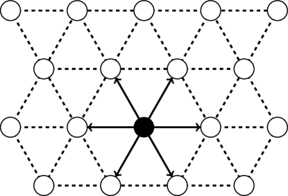
Figure 1. The lattice and its canonical triangulation.

We identify a discrete displacement map $u:\Lambda\rightarrow\mathbb{R}^{m}$, $m=1,2,3$, with its continuous piecewise affine interpolant, with weak derivative $\nabla u$, which is also the pointwise derivative on each element $T\in\mathcal{T}$. For $m=1,2,3$, the spaces of displacements are defined as

$$\mathcal{U}_{0} :=\big{\{}u\,|\,\Lambda\rightarrow\mathbb{R}^{m}:{\rm supp}(\nabla u)\text{ is compact}\big{\}},\quad\text{and}$$

$$\dot{\mathcal{U}}^{1,2} :=\big{\{}u\,|\,\Lambda\rightarrow\mathbb{R}^{m}:\nabla u\in L^{2}\big{\}}.$$

We equip $\dot{\mathcal{U}}^{1,2}$ with the $H^{1}$-seminorm, $\|u\|_{\mathcal{U}^{1,2}}:=\|\nabla u\|_{L^{2}(\mathbb{R}^{2})}$. From [8] we know that $\mathcal{U}_{0}$ is dense in $\dot{\mathcal{U}}^{1,2}$ in the sense that, if $u\in\dot{\mathcal{U}}^{1,2}$, then there exist $u_{j}\in\mathcal{U}_{0}$ such that $\nabla u_{j}\rightarrow\nabla u$ strongly in $L^{2}$.

A homogeneous displacement is a map $u_{\sf F}:\Lambda\rightarrow\mathbb{R}^{m},u_{\sf F}(x):={\sf F}x$, where ${\sf F}\in\mathbb{R}^{m\times 2}$.

For a map $u:\Lambda\rightarrow\mathbb{R}^{m}$, we define the finite difference operator

$$D_{j}u(x) :=u(x+a_{j})-u(x),\quad x\in\Lambda,j\in\{1,2,...,6\},\quad\text{and}$$ (2.1)

$$Du(x) :=(D_{j}u(x))_{j=1}^{6}.$$

Note that $Du_{{\sf F}}(x)={\sf F}{\bm{a}}$.

2.1. 2D many-body nearest neighbour interactions

We assume that the atomistic interaction is described by a nearest-neighbour many-body site energy potential $V\in C^{r}(\mathbb{R}^{m\times 6})$,$r\geq 5$, with $V(\mathbf{0})=0$. Furthermore, we assume that $V$ satisfies the point symmetry

$$V((-g_{j+3})_{j=1}^{6})=V({\bm{g}})\quad\forall{\bm{g}}\in\mathbb{R}^{m\times 6}.$$

The energy of a displacement $u\in\mathcal{U}_{0}$, given by

$$\mathcal{E}^{\rm a}(u):=\sum_{\ell\in\Lambda}V(Du(\ell)),$$

is well-defined since the infinite sum becomes finite. To formulate a variational problem in the energy space $\dot{\mathcal{U}}^{1,2}$, we need the following lemma to extend $\mathcal{E}^{\rm a}$ to $\dot{\mathcal{U}}^{1,2}$.

Lemma 2.1. $\mathcal{E}^{\rm a}:(\mathcal{U}_{0},\|\nabla\cdot\|_{L^{2}})\rightarrow\mathbb{R}$ is continuous and has a unique continuous extension to $\dot{\mathcal{U}}^{1,2}$, which we still denote by $\mathcal{E}^{\rm a}$. Furthermore, the extended $\mathcal{E}^{\rm a}:(\dot{\mathcal{U}}^{1,2},\|\nabla\cdot\|_{L^{2}})\rightarrow\mathbb{R}$ is $r$-times continuously Fréchet differentiable.

Proof.

See Lemma 2.1 in [4]. ∎

We model a point defect by adding an external potential $f\in C^{r}(\dot{\mathcal{U}}^{1,2})$ with $\partial_{u(\ell)}f(u)=0$ for all $|\ell|\geq R_{f}$, where $R_{f}$ is some given radius (the defect core radius), and $f(u+c)=f(u)$ for all constants $c$. For example, we can think of $f$ modelling a substitutional impurity. See also [5, 7] for similar approaches.

We then seek the solution to

$$u^{\rm a}\in\arg\min\big{\{}\mathcal{E}^{\rm a}(u)-f(u)\,|\,u\in\dot{\mathcal{U}}^{1,2}\big{\}}.$$ (2.2)

For $u,\varphi,\psi\in\dot{\mathcal{U}}^{1,2}$ we define the first and second variations of $\mathcal{E}^{\rm a}$ by

$$\langle\delta\mathcal{E}^{\rm a}(u),\varphi\rangle :=\lim_{t\rightarrow 0}t^{-1}\left(\mathcal{E}^{\rm a}(u+t\varphi)-\mathcal{E}^{\rm a}(u)\right),$$

$$\langle\delta^{2}\mathcal{E}^{\rm a}(u)\varphi,\psi\rangle :=\lim_{t\rightarrow 0}t^{-1}\left(\langle\delta\mathcal{E}^{\rm a}(u+t\varphi),\psi\rangle-\langle\delta\mathcal{E}^{\rm a}(u),\psi\rangle\right).$$

We use analogous definitions for all energy functionals introduced in later sections.

2.2. The Cauchy–Born Approximation

The Cauchy–Born strain energy function, corresponding to the interatomic potential $V$ is

$$W(\mathsf{F}):=\frac{1}{\Omega_{0}}V(\mathsf{F}{\bm{a}}),\qquad\text{for }\mathsf{F}\in\mathbb{R}^{m\times 2},$$

where $\Omega_{0}:=\sqrt{3}/2$ is the volume of a unit cell of the lattice $\Lambda$. Thus $W(\mathsf{F})$ is the energy per volume of the homogeneous lattice $\mathsf{F}\Lambda$.

2.3. The G23 coupling method

Let $\mathcal{A}\subset\Lambda$ denote the set of all lattices sites for which we want to maintain full atomistic accuracy. We denote the set of interface lattice sites by

$$\mathcal{I}:=\big{\{}\ell\in\Lambda\setminus\mathcal{A}\,\big{|}\,\ell+a_{j}\in\mathcal{A}\text{ for some }j\in\{1,\dots,6\}\big{\}}$$

and we denote the remaining lattice sites by $\mathcal{C}:=\Lambda\setminus(\mathcal{A}\cup\mathcal{I})$. Let $\Omega_{\ell}$ be the Voronoi cell associated with site $\ell$. We define the continuum region $\Omega^{\rm c}:=\mathbb{R}^{2}\setminus\bigcup_{\ell\in\mathcal{A}\cup\mathcal{I}}\Omega_{\ell}$; see Figure 2.

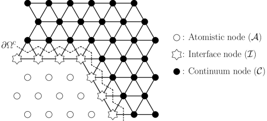
Figure 2. The domain decomposition with a layer of interface atoms.

A general form for the GRAC-type a/c coupling energy [3, 12] is

$$\mathcal{E}^{\rm ac}(u)=\sum_{\ell\in\mathcal{A}}V(Du(\ell))+\sum_{\ell\in\mathcal{I}}V\left((\mathcal{R}_{\ell}D_{j}u(\ell))_{j=1}^{6}\right)+\int_{\Omega^{\rm c}}W(\nabla u(x))\,{\rm d}x,$$

where $\mathcal{R}_{\ell}D_{j}u(\ell):=\sum_{i=1}^{6}C_{\ell,j,i}D_{i}u(\ell)$. The parameters $C_{\ell,j,i}$ are to be determined in order for the coupling scheme to satisfy the “patch tests”:

$\mathcal{E}^{\rm ac}$ is locally energy consistent if, for all ${\sf F}\in\mathbb{R}^{m\times 2}$,

$$V_{\ell}^{i}({\sf F}{\bm{a}})=V({\sf F}{\bm{a}})\quad\forall\ell\in\mathcal{I}.$$ (2.3)

$\mathcal{E}^{\rm ac}$ is force consistent if, for all ${\sf F}\in\mathbb{R}^{m\times 2}$,

$$\delta\mathcal{E}^{\rm ac}(u_{\sf F})=0,\quad\text{where}\quad u_{\sf F}(x):={\sf F}x.$$ (2.4)

$\mathcal{E}^{\rm ac}$ is patch test consistent if it satisfies both (2.3) and (2.4).

For the sake of brevity of notation we will often write $V^{i}_{\ell}(Du(\ell)):=V\left((\mathcal{R}_{\ell}D_{j}u(\ell))_{j=1}^{6}\right)$. Following [12] we make the following standing assumption (see Figure 3 for examples).

(A0) Each vertex $\ell\in\mathcal{I}$ has exactly two neighbours in $\mathcal{I}$, and at least one neighbour in $\mathcal{C}$.

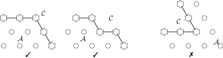
Figure 3. The first two configurations are allowed. The third configuration is not allowed as the interface atom at the corner has no nearest neighbour in the continuum region, and should instead be taken as an atomistic site.

Under this assumption, the geometry reconstruction operator $\mathcal{R}_{\ell}$ is then defined by

$$\mathcal{R}_{\ell}D_{j}y(\ell) :=(1-\lambda_{\ell,j})D_{j-1}y(\ell)+\lambda_{\ell,j}D_{j}y(\ell)+(1-\lambda_{\ell,j})D_{j+1}y(\ell),$$

$$\lambda_{x,j} :=\left\{\begin{array}[]{rl}2/3,&x+a_{j}\in\mathcal{C}\\ 1,&\text{otherwise}\end{array}\right.;$$

see Figure 4. The resulting coupling method is called G23 and the corresponding energy functional $\mathcal{E}^{\rm g23}$. This choice of coefficients (and only this choice) leads to patch test consistency (2.3) and (2.4).

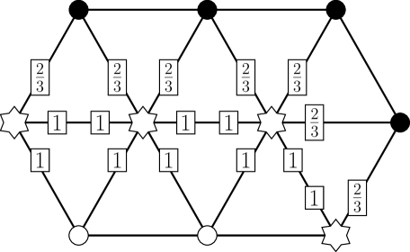
Figure 4. The geometry reconstruction coefficents $\lambda_{x,j}$ at the interface sites.

For future reference we decompose the canonical triangulation $\mathcal{T}$ as follows:

$$\mathcal{T}_{\mathcal{A}}: =\{T\in\mathcal{T}\,|\,T\cap(\mathcal{I}\cup\mathcal{C})=\emptyset,\},$$ (2.5)

$$\mathcal{T}_{\mathcal{C}}: =\{T\in\mathcal{T}\,|\,T\cap(\mathcal{I}\cup\mathcal{A})=\emptyset,\}\quad\text{and}$$

$$\mathcal{T}_{\mathcal{I}}: =\mathcal{T}\setminus(\mathcal{T}_{\mathcal{C}}\cup\mathcal{T}_{\mathcal{A}}).$$

2.4. Notation for a P$2$ finite element scheme

In the atomistic and interface regions, the interactions are represented by discrete displacement maps, which are identified with their linear interpolant. Here, we identify the displacement map with its P1 interpolant. No approximation error is committed.

On the other hand, in the continuum region where the interactions are approximated by the Cauchy–Born energy, we could increase the accuracy by using P$p$-FEM with $p>1$. In later sections we will review that the Cauchy–Born approximation yields a 2nd-order error, whereas employing the P1-FEM in the continuum region would reduce the accuracy to first order. In fact, we will show in that, with optimized mesh grading, P2-FEM is sufficient to obtain a convergence rate that cannot be improved by other choices of continuum discretisations. High-order P$p$-FEM with $p>2$ will increase the computational costs but yield the same error convergence rate (see § 3.5).

Let $K>0$ denote the inner radius of the atomistic region,

$$K:=\sup\big{\{}r>0\,|\,\mathcal{B}_{r}\cap\Lambda\subset\mathcal{A}\big{\}},$$

where $\mathcal{B}_{r}$ denotes the ball of radius $r$ centred at $0$. In order for the defect to be contained in the atomistic region we assume throughout that $K\geq R_{f}$.

Let $\Omega_{h}$ denote the entire computational domain and $N>0$ denote the inner radius of $\Omega_{h}$, i.e.,

$$N:=\sup\big{\{}r>0\,|\,\mathcal{B}_{r}\subset\Omega_{h}\big{\}}.$$

Let $\mathcal{T}_{h}$ be a finite element triangulation of $\Omega_{h}$ which satisfies, for $T\in\mathcal{T}_{h}$,

$$T\cap(\mathcal{A}\cup\mathcal{I})\neq\emptyset\quad\Rightarrow\quad T\in\mathcal{T}.$$

In other words, $\mathcal{T}_{h}$ and $\mathcal{T}$ coincide in the atomistic and interface regions, whereas in the continuum region the mesh size may increase towards the domain boundary. The optimal rate at which the mesh size increases will be determined in later sections.

We note that the concrete construction of $\mathcal{T}_{h}$ will be based on the choice of the domain parameters $K$ and $N$; hence, when emphasizing this dependence, we will write $\mathcal{T}_{h}(K,N)$. We assume throughout that the family $(\mathcal{T}_{h}(K,N))_{K,N}$ is uniformly shape-regular, i.e., there exists $c>0$ such that,

$${\rm diam}(T)^{2}\leq c|T|,\quad\forall T\in\mathcal{T}_{h}(K,N),\forall K\leq N.$$ (2.6)

This assumption eliminates the possibility of extreme angles on elements, which would deteriorate the constants in finite element interpolation error estimates. For the most part we will again drop the parameters from the notation by writing $\mathcal{T}_{h}\equiv\mathcal{T}_{h}(K,N)$ but implicitly will always keep the dependence.

Similar to (2.5), we define the atomistic, interface and continuum elements as $\mathcal{T}_{h}^{a},\mathcal{T}_{h}^{i}$ and $\mathcal{T}_{h}^{c}$, respectively. Note that $\mathcal{T}_{h}^{a}=\mathcal{T}_{\mathcal{A}}$ and $\mathcal{T}_{h}^{i}=\mathcal{T}_{\mathcal{I}}$. We also let $\mathcal{N}_{h}$ denote the number of degrees of freedom of $\mathcal{T}_{h}$.

We define the finite element space of admissible displacements as

$$\mathcal{U}_{h}:=\big{\{}u\in C(\mathbb{R}^{2};\mathbb{R}^{m})\,| {\rm{supp}}(u)\subset\Omega_{h},u|_{T}\in\mathbb{P}^{1}(T)\text{ for }T\subset\mathcal{T}_{h}^{a}\cup\mathcal{T}_{h}^{i}\,\text{ and}$$ (2.7)

$$u|_{T}\in\mathbb{P}^{2}(T)\text{ for }T\subset\mathcal{T}_{h}^{c}\big{\}}.$$

In defining $\mathcal{U}_{h}$ we have made two approximations to the class of admissible displacements: (1) truncation to a finite computational domain and (2) finite element coarse-graining.

The computational scheme is to find

$$u^{\rm g23}_{h}\in\arg\min\big{\{}\mathcal{E}^{\rm g23}(u_{h})-f(u_{h})\,|\,u_{h}\in\mathcal{U}_{h}\big{\}}.$$ (2.8)

Remark 2.2. $\mathcal{U}_{h}$ is embedded in $\mathcal{U}_{0}$ via point evaluation. Through this identification, $f(u_{h})$ is well-defined for all $u_{h}\in\mathcal{U}_{h}$.

We will make this identification only when we evaluate $f(u_{h})$. The reason for this is a conflict when interpreting elements $u_{h}$ as lattice functions is that we identify lattice functions with their continuous interpolants with respect to the canonical triangulation $\mathcal{T}$, which would be different from the function $u_{h}$ itself. However, for the evaluation of $f(u_{h})$ this issue does not arise. ∎

3. Summary of results

3.1. Regularity of $u^{\rm a}$

The approximation error analysis in later sections requires estimates on the decay of the elastic fields away from the defect core. These results follow from a natural stability assumption:

(A1) The atomistic solution is strongly stable, that is, there exists $C_{0}>0$,

$$\langle\delta^{2}\mathcal{E}^{{\rm a}}(u^{\rm a})\varphi,\varphi\rangle\geq C_{0}\|\nabla\varphi\|^{2}_{L^{2}},\quad\forall\varphi\in\dot{\mathcal{U}}^{1,2},$$ (3.1)

where $u^{\rm a}$ is a solution to (2.2).

Corollary 3.1. Suppose that (A1) is satisfied, then there exists a constant $C>0$ such that, for $1\leq j\leq r-2$,

$$|D^{j}u^{\rm a}(\ell)|\leq C|\ell|^{-1-j}.$$

Proof.

See Theorem 2.3 in [4]. ∎

3.2. Stability

In [9] it is shown that there is a “universal” instability in 2D interfaces for QNL-type a/c couplings: it is impossible to prove in full generality that $\delta^{2}\mathcal{E}^{\rm g23}(u^{\rm a})$ is a positive definite operator, even if we assume (3.1). Indeed, this potential instability is universal to a wide class of generalized geometric reconstruction methods. However, it is rarely observed in practice. To circumvent this difficulty, we make the following standing assumption:

(A2) The homogeneous lattice is strongly stable under the G23 approximation, that is, there exists $C^{\rm g23}_{0}>0$ which is independent of $K$ such that, for $K$ sufficiently large,

$$\langle\delta^{2}\mathcal{E}^{\rm g23}(0)\varphi_{h},\varphi_{h}\rangle\geq C^{\rm g23}_{0}\|\nabla\varphi_{h}\|^{2}_{L^{2}},\quad\forall\varphi_{h}\in\mathcal{U}_{h}.$$ (3.2)

Since (3.2) does not depend on the solution it can be tested numerically. But a precise understanding under which conditions (3.2) is satisfied is still missing. In [9] a method of stabilizing 2D QNL-type schemes with flat interfaces is introduced, which could replace this assumption, however we are not yet able to extend this stabilizing method for interfaces with corners, such as the configurations discussed in this paper.

3.3. Main results

To state the main results it is convenient to employ a smooth interpolant to measure the regularity of lattice functions. In Lemma 6.1, we define such an interpolant $\tilde{u}\in C^{2,1}(\mathbb{R}^{2})$ for $u\in\mathcal{U}_{0}$, for which there exists a universal constant $\tilde{C}$ such that, for all $q\in[1,\infty]$, $0\leq j\leq 3$,

$$|D^{j}u(\ell)|\leq\tilde{C}\|\nabla^{j}\tilde{u}\|_{L^{1}(\omega_{\ell})}\quad\text{and}\quad\|\nabla^{j}\tilde{u}\|_{L^{q}(T)}\leq\tilde{C}\|D^{j}u\|_{\ell^{q}(\Lambda\cap T)}$$

where $\omega_{\ell}:=\ell+{\sf A}(-1,1)^{2}$.

3.3.1. Consistency error estimate

In (5.6) we define a quasi-best approximation operator $\Pi_{h}:\mathcal{U}_{0}\rightarrow\mathcal{U}_{h}$, which truncates an atomistic displacement to enforce the homogeneous Dirichlet boundary condition, and then interpolates it onto the finite element mesh.

Our main result is the following consistency error estimate.

Theorem 3.2. If $u^{\rm a}$ is a solution to (2.2) then we have, for all $\varphi_{h}\in\mathcal{U}_{h}$,

$$\langle\delta\mathcal{E}^{\rm g23}(\Pi_{h}u^{\rm a}),\varphi_{h}\rangle\lesssim \bigg{(}\|\nabla^{2}\tilde{u}^{{\rm a}}\|_{L^{2}(\Omega^{\rm i})}+\|\nabla^{3}\tilde{u}^{{\rm a}}\|_{L^{2}(\Omega^{\rm c})}+\|\nabla^{2}\tilde{u}^{{\rm a}}\|^{2}_{L^{4}(\Omega^{\rm c})}$$ (3.3)

$$+\|h^{2}\nabla^{3}\tilde{u}^{{\rm a}}\|_{L^{2}(\Omega_{h}^{\rm c})}+\|\nabla\tilde{u}^{{\rm a}}\|_{L^{2}(\mathbb{R}^{2}\setminus\mathcal{B}_{N/2})}$$

$$+N^{-1}\|h^{2}\nabla^{2}\tilde{u}\|_{L^{2}(\mathcal{B}_{N}\setminus B_{N/2})}\bigg{)}\|\nabla\varphi_{h}\|_{L^{2}(\mathbb{R}^{2}\setminus\Omega^{\rm a})},$$

where $\Omega_{h}^{{\rm c}}$ corresponds to the continuum region of $\Omega_{h}$, and $h(x):=\text{\rm diam}(T)$ with $x\in T\in\mathcal{T}_{h}$.

3.3.2. Optimizing the approximation parameters

Before we estimate the error $\|\nabla u^{\rm a}-\nabla u_{h}\|_{L^{2}}$, we optimize the approximation parameters in the computational scheme. This means that the radius $K$ of the atomistic region, the radius $N$ of the entire computational domain and the mesh size $h$ should satisfy certain balancing relations. We only outline the result of this optimisation and refer to § 6.7 for the details.

Due to the decay estimates on $\tilde{u}^{\rm a}$ the dominating terms in (3.3) turn out to be

$$\|\nabla^{2}\tilde{u}^{{\rm a}}\|_{L^{2}(\Omega^{\rm i})}\qquad\text{and}\qquad\|\nabla\tilde{u}^{{\rm a}}\|_{L^{2}(\mathbb{R}^{2}\setminus\mathcal{B}_{N/2})}.$$ (3.4)

(We will see momentarily that the mesh size plays a minor role.) These two terms result from the nature of the coupling scheme and the far-field truncation error. In particular, both of these cannot be improved by the choice of discretisation of the Cauchy–Born model, e.g., order of the FEM. We also note that, if we had employed a P1-FEM, then the limiting factor would have been $\|h\nabla^{2}\tilde{u}^{\rm a}\|_{L^{2}(\Omega^{\rm c})}$.

We can balance the two terms in (3.4) by choosing $N\approx K^{5/2}$. It then remains to determine a mesh-size so that the finite element error contribution,

$$\|h^{2}\nabla^{3}\tilde{u}^{{\rm a}}\|_{L^{2}(\Omega^{\rm c}_{h})}\qquad\text{and}\qquad N^{-1}\|h^{2}\nabla^{2}\tilde{u}\|_{L^{2}(\mathcal{B}_{N}\setminus B_{N/2})}$$

remains small in comparison. We show that the scaling $h(x)\approx\left(\frac{|x|}{K}\right)^{\beta}$ is a suitable choice, with $1<\beta<3/2$, under which both terms become of order $O(K^{-3})$.

Thus, we have determined the approximation parameters $(K,N,h)$ in terms of a single parameter $K$. The quasi-optimal relations for P2-FEM discretisatino of the Cauchy–Born model are summarised in Table 1.

	$\beta$	$N$	$\mathcal{N}_{h}$	consistency error
P2-FEM	$\left(1,\frac{3}{2}\right)$	$K^{5/2}$	$K^{2}$	$K^{-5/2}$
P1-FEM	$\left(1,\frac{3}{2}\right)$	$K^{2}$	$K^{2}$	$K^{-2}$

Table 1. Quasi-optimal relations between approximation parameters for P2-GR23 and, for comparision, for P1-GR23.

Corollary 3.3. Suppose that $N,h$ satisfy the relations of Table 1, the consistency error estimate (3.3) in terms of the number of degrees of freedom $\mathcal{N}_{h}$ can be written as

$$\|\delta\mathcal{E}^{\rm g23}(\Pi_{h}u^{\rm a})\|_{\mathcal{U}^{-1,2}}\lesssim\mathcal{N}_{h}^{-5/4}.$$ (3.5)

3.3.3. Error estimate

To complete our summary of results, we now use the Inverse Function Theorem to obtain error estimates for the strains and the energy.

Theorem 3.4. Suppose that (A0), (A1) and (A2) are satisfied and that the quasi-optimal scaling of $N,h$ from Table 1 is satisfied. Then, for sufficiently large atomistic region size $K$, a solution $u^{\rm g23}_{h}$ to (2.8) exists which satisfies the error estimates

$$\|\nabla u^{\rm a}-\nabla u^{\rm g23}_{h}\|_{L^{2}} \lesssim\mathcal{N}_{h}^{-5/4},\quad\text{and}$$ (3.6)

$$\big{|}[\mathcal{E}^{\rm a}(u^{\rm a})-f(u^{\rm a})]-[\mathcal{E}^{\rm g23}(u^{\rm g23}_{h})-f(u^{\rm g23})]\big{|} \lesssim\mathcal{N}_{h}^{-7/4},$$ (3.7)

where $\mathcal{N}_{h}$ is the number of degrees of freedom.

3.4. Setup of the numerical tests

For our numerical tests, we consider an anti-plane displacement $u:\Lambda\rightarrow\mathbb{R}$. We choose a hexagonal atomistic region $\Omega^{\rm a}$ with side length $K$ and one layer of atomistic sites outside $\Omega^{\rm a}$ as the interface. To construct the finite element mesh, we add hexagonal layers of elements such that, for each layer $j$, $h(\text{layer }j)=(h(\text{layer }j-1)/K)^{\beta}$, with $\beta=1.4$; see Figure 5. The procedure is terminated once the radius of the domain exceeds $N=\lceil K^{5/2}\rceil$. This construction guarantees the quasi-optimal approximation parameter balance to optimise the P2-FEM error. The derivation is given in Section 6.7.

In our tests we compare the P2-G23 method against

• a pure atomistic model with clamped boundary condition: the construction of the domain is as in the P2-G23 method, but without continuum region;

• a P1-G23 method: the construction is again identical to that of the P2-G23 method, but the P2-FEM in the definition of $\mathcal{U}_{h}$ is replaced by a P1-FEM. The same mesh scaling as for P2 is used (see also [3] where this is shown to be quasi-optimal).

The site potential is given by a nearest-neighbour embedded atom toy model,

$$V(Du):=G\left(\sum_{i=1}^{6}\rho(D_{i}u(\ell))\right)$$

with $G(s):=s+\frac{1}{2}s^{2}$ and $\rho(r):=\sin^{2}(r\pi)$. This is the anti-plane toy model as the one used in [4].

The external potential is defined by $\langle f,u\rangle=10(u(0,0)-u(1,0))$, which can be thought of as an elastic di-pole. A steepest descent method, preconditioned with a finite element Laplacian and fixed (manually tuned) step-size, is used to find a minimizer $u^{\rm g23}_{h}$ of $\mathcal{E}^{g23}(u)-f(u)$, using $u_{h}=0$ as the starting guess.

In order to compare the errors, we use a comparison solution with atomistic region size $3K$ and other computational parameters scaled as above.

The numerical results, with brief discussions, are shown in Figures 6–9. The two most important observations are the following:

• the numerical tests confirm the analytical predictions for the energy-norm error, but the experimental rates for the energy error are better than the analytical rates. Similar observations were also made in [4].

• With our specific setup, the improvement of the P2-GR23 over P1-GR23 is clearly observed when plotting the error against $\#\mathcal{A}\propto\mathcal{N}_{h}$, but when plotted against $\mathcal{N}_{h}$ the improvement is only seen in the asymptotic regime. This indicates that further work is required, such as a posteriori adaption, to optimise the P2-GR23 in the pre-asymptotic regime as well.

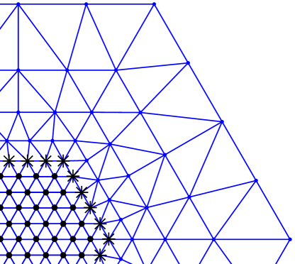
Figure 5. An example of the computatioanl mesh. The the vertices marked by ”•” are the atomistic sites; the vertices marked by ”$\ast$” are the interface sites.

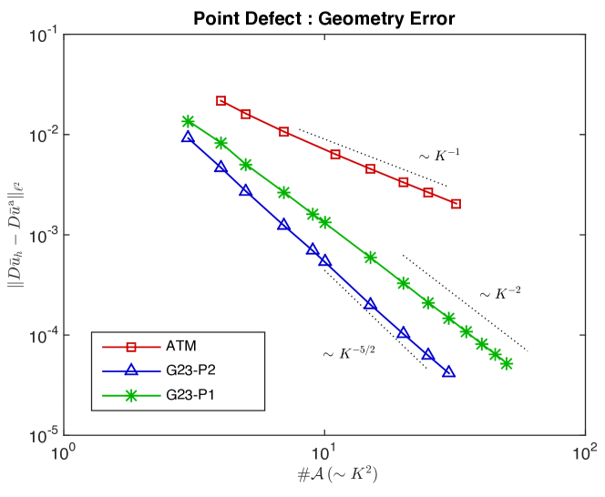
Figure 6. Error in energy norm plotted against $\#\mathcal{A}$. We clearly observe the predicted rate of convergence.

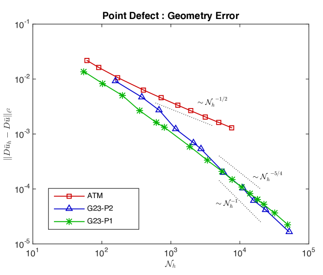
Figure 7. Error in energy norm plotted against the number of degrees of freedom. The improvement of P2-FEM is now only seen asymptotically.

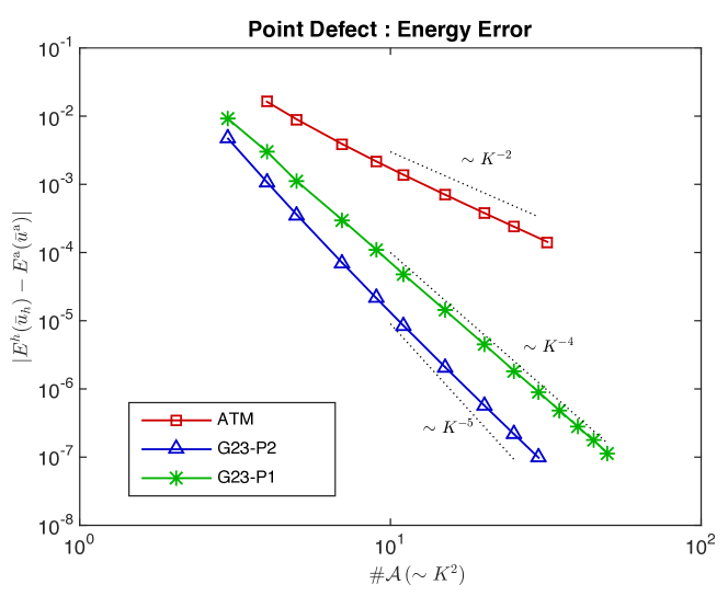
Figure 8. The energy error plotted against $\#\mathcal{A}$. The observed rate of convergence is better than the rate predicted in Theorem 3.3.3.

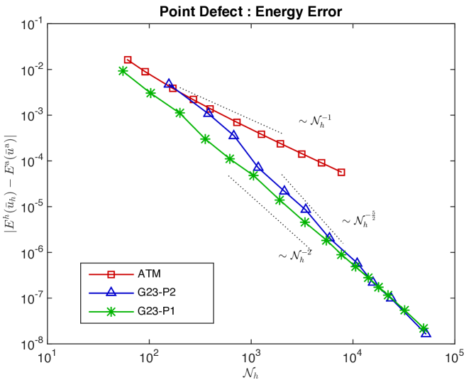
Figure 9. The energy error plotted against the number of degrees of freedom. The improvement of P2-FEM over P1-FEM can again only be observed asymptotically.

3.5. Extension to high-order FEM

If we apply higher-order FEM in the continuum region, then to extend our error analysis we would need a smooth interpolant of $u\in\mathcal{U}_{0}$ with higher regularity than $\tilde{u}\in C^{2,1}(\mathbb{R}^{2})$. A suitable extension given in [5] is, for arbitrary $n$, a $C^{n,1}$ piecewise polynomial of degree $2n+1$ with properties analogous to those stated in Lemma 6.1. The resulting higher-order decay rate $|\nabla^{j}\tilde{u}^{\rm a}(x)|\lesssim|x|^{-j-1}$ indicates that the use of high-order FEM could be beneficial.

However, as we have pointed out in § 3.3.2, if we employ the mesh grading $h(x)=(|x|/K)^{\beta}$ with $1<\beta<3/2$ in the continuum region, the total approximation error cannot be improved by using P$p$-FEM with $p>2$, since the dominating term is the interface error $\|\nabla^{2}\tilde{u}^{\rm a}\|_{L^{2}(\Omega^{\rm i})}$ for $p\geq 2$, which results from the construction of G23 coupling and is not affected by the choice of FEM.

If we consider a coarser mesh for high-order FEM in hopes of reducing the number of degrees of freedom, i.e., choosing $\beta\geq 3/2$, then applying analogous calculations to those in §6.7 gives us the following result:

Employing P$p$-FEM with $p>2$, in order to match the convergence rate of the Cauchy–Born error term $\|\nabla^{3}\tilde{u}^{\rm a}\|_{L^{2}(\Omega^{\rm c})}\sim K^{-3}$, the highest mesh coarsening rate is

$$\beta=\frac{5}{3}-\frac{1}{3p}.$$

This means that the optimal mesh grading that P$p$-FEM can achieve without compromising accuracy is no greater than $\frac{5}{3}$. However, in that case, the number of degrees of freedom is always $\mathcal{O}(K^{2})$.

In summary, despite the possibility of (slightly) reducing the number of degrees of freedom, considering its computational complexity, we conclude that higher-order FEM is not worthwhile to pursue. However, we emphasize that this conclusion would need to be revisited if a coupling method with higher-order interface error as well as continuum model error could be devised.

4. Conclusion

We obtained a sharp energy-norm error estimate for the G23 coupling method with P2-FEM discretisation of the continuum model. Furthermore, we demonstrated that, with P1-FEM discretisation the FEM coarsening error is the dominating term in the consistency error estimate, whereas for P2-FEM discretisation the interface error becomes the dominating term. In particular, a P2-FEM discretisation yields a more rapid decay of the error. Crucially though, since for P$p$-FEM with $p\geq 2$ the interface contribution dominates the total error the P2-FEM is already optimal. That is, increasing to $p>2$ will not improve the rate of convergence, but increase the computational cost and algorithmic complexity.

Numerically, we observe that the improvement of P2-GR23 over P1-GR23 is only modest at low $\mathcal{N}_{h}$, hence a P2-GR23 scheme would be primarily of interest if high accuracy of the solution is required. However, our numerical results indicate that there is scope for further optimisation, using a posteriori type techniques.

While our estimates for the error in energy-norm are sharp, our numerical results show the estimates for the energy errors are suboptimal. We hightlight the leading term in the error analysis which overestimate the error in Section 7.2. We are unable, at present, to obtain an optimal energy error estimate. This appears to be an open problem throughout the literature on hybrid atomistic multi-scale schemes; see e.g. [4].

In summary we conclude that using P2-FEM is a promising improvement to the efficiency of a/c coupling methods, but that some further work, both theoretical and for its implementation may be need to exploit its full potential.

5. Reduction to consistency

Assuming the existence of an atomistic solution $u^{\rm a}$, we seek to prove the existence of $u_{h}^{\rm g23}\in\mathcal{U}_{h}$ satisfying

$$\langle\delta\mathcal{E}^{\rm g23}(u^{\rm g23}_{h}),\varphi_{h}\rangle=\langle\delta f(u_{h}^{\rm g23}),\varphi_{h}\rangle,\quad\text{for all }\varphi_{h}\in\mathcal{U}_{h},$$ (5.1)

and to estimate the $\|u^{\rm a}-u^{\rm g23}_{h}\|$ in a suitable norm.

The error analysis consists of consistency and stability estimates. Once these are established we apply the following theorem to obtain the existence of a solution $u_{h}^{\rm g23}$ and the error estimate. The proof of this theorem is standard and can be found in various references, e.g. [13, Lemma 2.2].

Theorem 5.1 (The inverse function theorem). Let $\mathcal{U}_{h}$ be a subspace of $\mathcal{U}$, equipped with $\|\nabla\cdot\|_{L^{2}}$, and let $\mathcal{G}_{h}\in C^{1}(\mathcal{U}_{h},\mathcal{U}_{h}^{*})$ with Lipschitz-continuous derivative $\delta\mathcal{G}_{h}$:

$$\|\delta\mathcal{G}_{h}(u_{h})-\delta\mathcal{G}_{h}(v_{h})\|_{\mathcal{L}}\leq M\|\nabla u_{h}-\nabla v_{h}\|_{L^{2}}\quad\text{for all }u_{h},v_{h}\in\mathcal{U}_{h},$$

where $\|\cdot\|_{\mathcal{L}}$ denotes the $\mathcal{L}(\mathcal{U}_{h},\mathcal{U}_{h}^{*})$-operator norm.

Let $\bar{u}_{h}\in\mathcal{U}_{h}$ satisfy

$$\|\mathcal{G}_{h}(\bar{u}_{h})\|_{\mathcal{U}_{h}^{*}} \leq\eta,$$ (5.2)

$$\langle\delta\mathcal{G}_{h}(\bar{u}_{h})v_{h},v_{h}\rangle \geq\gamma\|\nabla v_{h}\|^{2}_{L^{2}}\quad\text{ for all }v_{h}\in\mathcal{U}_{h},$$ (5.3)

such that $M,\eta,\gamma$ satisfy the relation

$$\frac{2M\eta}{\gamma^{2}}<1.$$

Then there exists a (locally unique) $u_{h}\in\mathcal{U}_{h}$ such that $\mathcal{G}_{h}(u_{h})=0$,

$$\|\nabla u_{h}-\nabla\bar{u}_{h}\|_{L^{2}} \leq 2\frac{\eta}{\gamma},\quad\text{and}$$

$$\langle\delta\mathcal{G}_{h}(u_{h})v_{h},v_{h}\rangle \geq\left(1-\frac{2M\eta}{\gamma^{2}}\right)\gamma\|\nabla v_{h}\|^{2}_{L^{2}}\quad\text{for all }v_{h}\in\mathcal{U}_{h}.$$

To ensure Dirichlet boundary conditions, we adapt the approximation map defined in [4]. Let $\mu\in C^{1}(\mathbb{R}^{2})$ be a cut-off function such that

$$\mu(x)=\left\{\begin{array}[]{l l}1&0\leq x\leq\frac{1}{2},\\ 0&x\geq 1.\end{array}\right.$$

For $u:\Lambda\rightarrow\mathbb{R}^{m}$, define

$$\mathcal{L}u(x):=\mu\left(\frac{|x|}{N}\right)\left(\tilde{u}(x)-a_{u}\right),\text{ where }a_{u}:=\frac{1}{|B_{N}\setminus B_{N/2}|}\int_{B_{N}\setminus B_{N/2}}\tilde{u}(y)\,{\rm d}y.$$ (5.4)

Let $\nu_{T,i},i=1,2,3$ be the vertices of $T$ and $m_{e}$ be the mid-point of an edge $e$. Then, the set of all active P2 finite element nodes is given by

$$\mathcal{N}_{h}:=\{\nu_{T,i}\,|\,T\in\mathcal{T}_{h},i=1,2,3\}\cup\{m_{e}\,|\,e=T_{1}\cap T_{2},T_{1},T_{2}\in\mathcal{T}^{c}_{h}\}.$$

This includes all P1 nodes as well as the P2 nodes (edge midpoints) associatd with edges entirely in the P2 region.

Furthermore, let $I^{2}_{h}:C(\mathbb{R}^{2};\mathbb{R}^{m})\rightarrow\mathcal{U}_{h}$ be the interpolation operator such that, for $g\in C(\mathbb{R}^{2};\mathbb{R}^{m})$, $I^{2}_{h}(g)|_{T}\in\mathbb{P}^{1}(T)$ for $T\subset\mathcal{T}_{h}^{a}\cup\mathcal{T}_{h}^{i}$, $I^{2}_{h}(g)|_{T}\in\mathbb{P}^{2}(T)\text{ for }T\subset\mathcal{T}_{h}^{c}$, and

$$I^{2}_{h}(g)(x)=g(x)\qquad\text{ for all $x\in\mathcal{N}_{h}$}.$$

Remark 5.2. We also introduce ghost nodes on the edges shared by interface and continuum elements:

$$\mathcal{N}_{h}^{g}:=\{m_{e}\,|\,e=T_{1}\cap T_{2},T_{1}\in\mathcal{T}^{i}_{h},T_{2}\in\mathcal{T}^{c}_{h}\}.$$ (5.5)

Then, for $x\in\mathcal{N}_{h}^{g}$, $I^{2}_{h}(g)(x)=(g(\nu_{x}^{1})+g(\nu_{x}^{2}))/2$, where $\nu_{x}^{1}$ and $\nu_{x}^{2}$ are the vertices of the edge on which $x$ lies. Hence, the $P^{1}$ and $P^{2}$ interpolants coincide on $\mathcal{N}_{h}^{g}$. ∎

We can now define the projection map (quasi-best approximation operator) $\Pi_{h}:\mathcal{U}_{0}\rightarrow\mathcal{U}_{h}$ as

$$\Pi_{h}:=I^{2}_{h}\circ\mathcal{L}.$$ (5.6)

5.1. Stability

To put Theorem 5 (Inverse Function Theorem) into our context, let

$$\mathcal{G}_{h}(v):=\delta\mathcal{E}^{\rm g23}(v)-\delta f(v)\quad\text{and}\quad\bar{u}_{h}:=\Pi_{h}u^{\rm a}.$$

To make (5.2) and (5.3) concrete we will show that there exist $\eta,\gamma>0$ such that, for all $\varphi_{h}\in\mathcal{U}_{h}$,

$$\langle\delta\mathcal{E}^{\rm g23}(\Pi_{h}u^{\rm a}),\varphi_{h}\rangle-\langle\delta f(\Pi_{h}u^{\rm a}),\varphi_{h}\rangle \leq\eta\|\nabla\varphi_{h}\|_{L^{2}},\quad(consistency)$$

$$\langle\delta^{2}\mathcal{E}^{\rm g23}(\Pi_{h}u^{\rm a})\varphi_{h},\varphi_{h}\rangle-\langle\delta^{2}f(\Pi_{h}u^{\rm a})\varphi_{h},\varphi_{h}\rangle \geq\gamma\|\nabla\varphi_{h}\|^{2}_{L^{2}}.\quad(stability)$$

Ignoring some technical requirements, the inverse function theorem implies that, if $\eta/\gamma$ is sufficiently small, then there exists $u^{\rm g23}_{h}\in\mathcal{U}_{h}$ such that

$$\langle\delta\mathcal{E}^{\rm g23}(u_{h}^{\rm g23}),\varphi_{h}\rangle-\langle\delta f(u_{h}^{\rm g23}),\varphi_{h}\rangle=0,\quad\forall\varphi_{h}\in\mathcal{U}_{h},\quad\text{and}$$

$$\|\nabla u^{\rm g23}_{h}-\nabla\Pi_{h}u^{\rm a}\|_{L^{2}}\leq 2\frac{\eta}{\gamma}.$$

Finally adding the best approximation error $\|\nabla\Pi_{h}u^{\rm a}-\nabla u^{\rm a}\|_{L^{2}}$ gives the error estimate

$$\|\nabla u^{\rm g23}_{h}-\nabla u^{\rm a}\|_{L^{2}}\leq\|\nabla\Pi_{h}u^{\rm a}-\nabla u^{\rm a}\|_{L^{2}}+2\frac{\eta}{\gamma}$$

The Lipschitz and consistency estimates require assumptions on the boundedness of partial derivatives of $V$. For ${\bm{g}}\in\mathbb{R}^{m\times 6}$, define the first and second partial derivatives, for $i,j=1,\dots,6$, by

$$\partial_{j}V({\bm{g}}):=\frac{\partial V({\bm{g}})}{\partial g_{j}}\in\mathbb{R}^{m},\quad\text{and}\quad\partial_{i,j}V({\bm{g}}):=\frac{\partial^{2}V({\bm{g}})}{\partial g_{i}\partial g_{j}}\in\mathbb{R}^{m\times m},$$

and similarly for the third derivatives $\partial_{i,j,k}V({\bm{g}})\in\mathbb{R}^{m\times m\times m}$. We assume that the second and third derivatives are bounded

$$M_{2}: =\sum_{i,j=1}^{6}\sup_{{\bm{g}}\in\mathbb{R}^{m\times 6}}\sup_{\begin{subarray}{c}h_{1},h_{2}\in\mathbb{R}^{2},\\ |h_{1}|=|h_{2}|=1\end{subarray}}\partial_{i,j}V({\bm{g}})[h_{1},h_{2}]<\infty,\quad\text{and}$$ (5.7)

$$M_{3}: =\sum_{i,j,k=1}^{6}\sup_{{\bm{g}}\in\mathbb{R}^{m\times 6}}\sup_{\begin{subarray}{c}h_{1},h_{2},h_{3}\in\mathbb{R}^{2},\\ |h_{1}|=|h_{2}|=|h_{3}|=1\end{subarray}}\partial_{i,j,k}V({\bm{g}})[h_{1},h_{2},h_{3}]<\infty.$$ (5.8)

With the above bounds it is easy to show that

$$\sum_{i=1}^{6}|\partial_{i}V({\bm{g}})-\partial_{i}V({\bm{h}})|\leq M_{2}\max_{j=1,\dotsc,6}|g_{j}-h_{j}|,\quad\text{for }{\bm{g}},{\bm{h}}\in\mathbb{R}^{m\times 6}.$$ (5.9)

From the bounds above we can obtain the following Lipschitz continuity and stability results.

Lemma 5.3. There exists $M>0$ such that

$$\|\delta\mathcal{G}_{h}(u_{h})-\delta\mathcal{G}_{h}(v_{h})\|_{\mathcal{L}}\leq M\|\nabla u_{h}-\nabla v_{h}\|_{L^{2}}\quad\text{for all }u_{h},v_{h}\in\mathcal{U}_{h}.$$ (5.10)

Proof.

The result follows directly from the global bounds of derivatives of $V$ and the fact that $f\in C^{k}(\dot{\mathcal{U}}^{1,2})$ and that $\delta f$ is compactly supported hence $\delta^{2}f$ is also Lipschitz. ∎

Lemma 5.4. Under the assumptions (A1) and (A2), if $\mathcal{G}_{h}(v):=\delta\mathcal{E}^{\rm g23}(v)-\delta f(v)$, then there exits $\gamma>0$ such that, when $K$ is sufficiently large,

$$\langle\delta\mathcal{G}_{h}(\Pi_{h}u^{\rm a})\varphi_{h},\varphi_{h}\rangle\geq\gamma\|\nabla\varphi_{h}\|^{2}_{L^{2}}\quad\text{ for all }\varphi_{h}\in\mathcal{U}_{h}.$$ (5.11)

Proof.

The proof of this result is a straightforward adaption of the proof of [5, Lemma 4.9], which is an analogous result for blending-type a/c coupling. ∎

6. Consistency estimate with a P2-FEM

6.1. Outline of the consistency estimate

We begin by decomposing the consistency error into

$$\langle\delta\mathcal{E}^{\rm g23}(\Pi_{h}u^{\rm a}),\varphi_{h}\rangle-\langle\delta f(\Pi_{h}u^{\rm a}),\varphi_{h}\rangle =\left\{\langle\delta\mathcal{E}^{\rm g23}(\Pi_{h}u^{\rm a}),\varphi_{h}\rangle-\langle\delta\mathcal{E}^{{\rm a}}(u^{\rm a}),\varphi\rangle\right\}$$

$$\quad+\left\{\langle\delta f(\Pi_{h}u^{\rm a}),\varphi_{h}\rangle-\langle\delta f(u^{\rm a}),\varphi\rangle\right\}$$

$$=:\eta_{\rm int}+\eta_{\rm ext},$$ (6.1)

where $\varphi_{h}\in\mathcal{U}_{h}$ is given and we can choose $\varphi\in\mathcal{U}_{0}$ arbitrarily.

For $\varphi_{h}\in\mathcal{U}_{h}$, $\varphi_{h}|_{T}\in\mathbb{P}^{2}(T)$ for $T\in\mathcal{T}_{h}^{c}$. But the test function $\varphi$ in $\langle\delta\mathcal{E}^{\rm a}(u^{\rm a}),\varphi\rangle$ is a piecewise linear lattice function. While we postpone the construction of $\varphi$, we will ensure that it is defined in such a way that $\varphi(\ell)=\varphi_{h}(\ell)$ for all $\ell\in\mathcal{A}\cup\mathcal{I}\cup\mathcal{I}^{+}$, where $\mathcal{I}^{+}$ is an extra layer of atomistic sites outside $\mathcal{I}$. With this assumption in place, we can further decompose $\eta_{\rm int}$ into the following parts,

$$\eta_{\rm int} =\int_{\Omega^{\rm c}}\partial_{\mathsf{F}}W(\nabla\tilde{u}^{\rm a}):(\nabla\varphi_{h}-\nabla\varphi)$$ (6.2)

$$\quad+\int_{\Omega^{\rm c}}(\partial_{\sf F}W(\nabla\Pi_{h}u^{\rm a})-\partial_{\mathsf{F}}W(\nabla\tilde{u}^{\rm a})):\nabla\varphi_{h}$$

$$\quad+\int_{\Omega^{\rm c}}\big{[}\partial_{\sf F}W(\nabla\tilde{u}^{\rm a})-\partial_{\sf F}W(\nabla{u}^{\rm a})\big{]}:\nabla\varphi$$

$$\quad+\langle\delta\mathcal{E}^{\rm g23}(u^{\rm a})-\delta\mathcal{E}^{\rm a}(u^{\rm a}),\varphi\rangle$$

$$=:\delta_{1}+\delta_{2}+\delta_{3}+\delta_{4},$$

where $\tilde{u}^{\rm a}$ is the smooth interpolant of $u^{\rm a}$ defined in Lemma 6.1 below. By $\nabla\varphi$ in $\delta_{1}$ we mean the gradient of the canonical linear interpolant of $\varphi$. To estimate $\delta_{2}$ we require an approximation error estimate for $\Pi_{h}u-u$. To estimate $\delta_{3}$ we will exploit the fact that the atomistic triangulation $\mathcal{T}$ is uniform to prove a super-convergence estimate. Finally, for the modelling error, $\delta_{4}$, we employ the techniques developed in [12].

To define the smooth interpolant $\tilde{u}^{\rm a}$, we use the construction from [5], namely a $C^{2,1}$-conforming multi-quintic interpolant. Although the interpolant defined in [5] is for lattice functions on $\mathbb{Z}^{2}$, we can use the linear transformation from $\mathbb{Z}^{2}$ to $\Lambda={\sf A}\mathbb{Z}^{2}$ to obtain a modified interpolant.

Lemma 6.1. (a) For each $u:\Lambda\rightarrow\mathbb{R}^{m}$, there exists a unique $\tilde{u}\in C^{2,1}(\mathbb{R}^{2};\mathbb{R}^{m})$ such that, for all $\ell\in\Lambda$,

$$\left.\tilde{u}\right|_{\ell+{\sf A}(0,1)^{2}} \text{ is a polynomial of degree 5},$$

$$\tilde{u}(\ell) =u(\ell),$$

$$\partial_{a_{i}}\tilde{u}(\ell) =\tfrac{1}{2}\left(u(\ell+a_{i})-u(\ell-a_{i})\right),$$

$$\partial_{a_{i}}^{2}\tilde{u}(\ell) =u(\ell+a_{i})-2u(\ell)+u(\ell-a_{i}),$$

where $i\in\{1,2\}$ and $\partial_{a_{i}}$ is the derivative in the direction of $a_{i}$.

(b) Moreover, for $q\in[1,\infty]$, $0\leq j\leq 3$,

$$\|\nabla^{j}\tilde{u}\|_{L^{q}(\ell+{\sf A}(1,0)^{2})}\lesssim\|D^{j}u\|_{\ell^{q}\left(\ell+{\sf A}\{-1,0,1,2\}^{2}\right)}\quad\text{and }\quad|D^{j}u(\ell)|\lesssim\|\nabla^{j}\tilde{u}\|_{L^{1}(\ell+{\sf A}(-1,1)^{2})},$$ (6.3)

where $D$ is the difference operator defined in (2.1). In particular,

$$\|\nabla\tilde{u}\|_{L^{q}}\lesssim\|\nabla u\|_{L^{q}}\lesssim\|\nabla\tilde{u}\|_{L^{q}},$$

where $u$ is identified with its piecewise affine interpolant.

Proof.

Let $v:\mathbb{Z}^{2}\rightarrow\mathbb{R}^{m}$ and $v(\xi):=u({\sf A}\xi)$ for all $\xi\in\mathbb{Z}$. Then [5, Lemma 1] shows that there exists a unique $\tilde{v}\in C^{2,1}(\mathbb{R}^{2};\mathbb{R}^{m})$ such that, for $\xi\in\mathbb{Z}^{2}$,

$$\left.\tilde{v}\right|_{\xi+(0,1)^{2}} \text{ is a polynomial of degree 5},$$

$$\tilde{v}(\xi) =v(\xi),$$

$$\partial_{e_{i}}\tilde{v}(\xi) =\tfrac{1}{2}\left(v(\xi+e_{i})-v(\xi-e_{i})\right),$$

$$\partial_{e_{i}}^{2}\tilde{v}(\xi) =v(\xi+e_{i})-2v(\xi)+v(\xi-e_{i})\quad i=1,2,$$

Defining $\tilde{u}(x):=\tilde{v}({\sf A}^{-1}x)$ for all $x\in\mathbb{R}^{2}$ proves part(a).

For part (b), [5, Lemma 1] establishes also that there exists a constant $C^{\prime}_{j}$ such that, for $\xi\in\mathbb{Z}^{2}$, $1\leq j\leq 3$, $q\in[1,\infty]$,

$$\|\nabla^{j}\tilde{v}\|_{L^{q}(\xi+(1,0)^{2})}\leq C^{\prime}_{j}\|\hat{D}^{j}v\|_{\ell^{q}\left(\xi+\{-1,0,1,2\}^{2}\right)},$$

where $\hat{D}$ represents the 4-stencil difference operator in $\mathbb{Z}^{2}$: let $\mathcal{R}:=\{\rho\in\mathbb{Z}^{2}\,|\,|\rho|=1\}$, then $\hat{D}v(\ell):=(\hat{D}_{\rho}v(\ell))_{\rho\in\mathcal{R}}$ with $\hat{D}_{\rho}v(\ell):=v(\ell+\rho)-v(\ell)$. After transformation, we have, for $\xi={\sf A}\ell\in\Lambda$,

$$\hat{D}v(\ell)=(D_{i}u(\xi))_{i=1,2,4,5}.$$

By adding the additional stencil elements $D_{3},D_{6}$ we obtain

$$C^{\prime\prime}_{j}\|\nabla^{j}\tilde{u}\|_{L^{q}(\xi+{\sf A}(1,0)^{2})} \leq\|\nabla^{j}\tilde{v}\|_{L^{q}(\ell+(1,0)^{2})}$$

$$\leq C^{\prime}_{{j}}\|\hat{D}^{j}v\|_{\ell^{q}\left(\ell+\{-1,0,1,2\}^{2}\right)}\leq C^{\prime\prime\prime}_{j}\|D^{j}u\|_{\ell^{q}\left(\xi+{\sf A}\{-1,0,1,2\}^{2}\right)},$$

where $C^{\prime\prime}_{j}$ and $C^{\prime\prime\prime}_{j}$ only depend on $j$. Writing $C:=\max_{1\leq j\leq 3}\left(\frac{C^{\prime\prime\prime}_{j}}{C^{\prime\prime}_{j}}\right)$ yields the first inequality of (6.3). Following a similar argument the second inequality also holds. ∎

6.2. Construction of $\varphi$ and estimation of $\delta_{1}$

Recall that

$$\delta_{1}:=\int_{\Omega^{\rm c}}\partial_{\mathsf{F}}W(\nabla\tilde{u}^{\rm a}):(\nabla\varphi_{h}-\nabla\varphi).$$

We adapt the modified quasi-interpolation operator introduced in [2] to approximate a test function $\varphi_{h}\in\mathcal{U}_{h}$. The advantage of this interpolation operator is that by using the setting of a partition of unity the approximation error has a local average zero. Consequently we can apply Poincaré inequality on patches to obtain local estimates.

We think of the construction of $\varphi$ as a Dirichlet boundary problem with the outer boundary $\partial\Omega_{h}$ and the inner boundary $\partial\Omega^{\rm c}$. Let $\phi_{\ell}$ be the piecewise linear hat-functions on the canonical triangulation $\mathcal{T}$ associated with $\ell\in\Lambda$. Define

$$\phi^{\rm PU}_{\ell}:=\frac{\phi_{\ell}}{\sum_{k\in\mathcal{C}\cap\Omega_{h}}\phi_{k}},\quad\forall\ell\in\mathcal{C},$$

where $\mathcal{C}$ is the continuum lattice sites as defined in §2.3. It is clear that $\{\phi^{\rm PU}_{\ell}\}_{\ell\in\mathcal{C}\cap\Omega_{h}}$ is a partition of unity.

Now we refer to [2] for the contruction of a linear interpolant of $\varphi_{h}\in\mathcal{U}_{h}$ . We shall define the interpolant as follows:

$$\Pi_{h}^{*}\varphi_{h}(x):=\varphi(x):=\varphi_{1}(x)+\varphi_{2}(x),\quad\forall x\in\mathbb{R}^{2},$$ (6.4)

where

$$\varphi_{1}(\ell) :=\left\{\begin{array}[]{rl}\varphi_{h}(\ell),&\ell\in\mathcal{A}\cup\mathcal{I}\cup\mathcal{I}^{+},\\ \frac{\int_{\mathbb{R}^{2}}\phi_{\ell}\varphi_{h}}{\int_{\mathbb{R}^{2}}\phi_{\ell}},&\ell\in\mathcal{C}\setminus\mathcal{I}^{+},\end{array}\right.$$

$$\varphi_{1}(x) :=\sum_{\ell\in\Lambda}\varphi_{1}(\ell)\phi_{\ell}(x),\quad\forall x\in\mathbb{R}^{2},$$

$$\varphi_{2}(\ell) :=\left\{\begin{array}[]{rl}\frac{\int_{\mathbb{R}^{2}}(\varphi_{h}-\varphi_{1})\phi_{\ell}^{\rm PU}}{\int_{\mathbb{R}^{2}}\phi_{\ell}},&\ell\in\mathcal{C}\setminus\mathcal{I}^{+},\\ 0,&\ell\in\mathcal{A}\cup\mathcal{I}\cup\mathcal{I}^{+},\end{array}\right.$$

$$\varphi_{2}(x) :=\sum_{\ell\in\Lambda}\varphi_{2}(\ell)\phi_{\ell}(x),\quad\forall x\in\mathbb{R}^{2}.$$

Observe that $\varphi_{h}$ and $\varphi$ both are supported on a finite domain, hence we can use Theorem 3.1 in [2] to conclude that

$$\|\nabla\varphi\|_{L^{2}(\mathbb{R}^{2})}\lesssim\|\nabla\varphi_{h}\|_{L^{2}(\mathbb{R}^{2})},\quad\forall\varphi_{h}\in\mathcal{U}_{h}.$$

Let $g:=-{\rm div}\,[\partial_{{\sf F}}W(\nabla\tilde{u}^{\rm a})]$. Then

$$\delta_{1}=\int_{\Omega^{\rm c}}g\cdot(\varphi_{h}-\varphi)\,{\rm d}x=\int_{\Omega^{\rm c}}g\cdot\left((\varphi_{h}-\varphi_{1})-\varphi_{2}\right)\,{\rm d}x$$

Since $\varphi_{2}$ is a piecewise-linear quasi-interpolant of $\varphi_{h}-\varphi_{1}$ as defined in [2], a direct consequence of Theorem 3.1 in [2] is that there exists $C>0$ such that, recalling $\Omega_{h}^{\rm a}:=\bigcup\mathcal{T}_{h}^{\rm a}$,

$$\delta_{1}\leq C\|\nabla(\varphi_{h}-\varphi_{1})\|_{L^{2}(\mathbb{R}^{2}\setminus\Omega_{h}^{\rm a})}\left(\sum_{\ell\in\mathcal{C}\cap\Omega_{h}}d_{\ell}^{2}\int_{w_{\ell}}\phi^{\rm PU}_{\ell}|g-\langle g\rangle_{\ell}|^{2}\,{\rm d}x\right)^{1/2},$$

where $w_{\ell}:={\rm supp}(\phi_{\ell})$, $\langle g\rangle_{\ell}:=1/|w_{\ell}|\int_{w_{\ell}}g(x)\,{\rm d}x$ and $d_{\ell}:={\rm diam}(w_{\ell})=1$. With the sharp Poincaré constant derived by [1] , we have

$$\int_{w_{\ell}}\phi^{\rm PU}_{\ell}|g-\langle g\rangle_{\ell}|^{2}\,{\rm d}x\leq\int_{w_{\ell}}|g-\langle g\rangle_{\ell}|^{2}\,{\rm d}x\leq\tfrac{1}{4}d^{2}_{\ell}\|\nabla g\|^{2}_{L^{2}(w_{\ell})}.$$

On the other hand, $\varphi_{1}$ is a standard quasi-interpolant of $\varphi_{h}$ in $\bigcup{\mathcal{T}_{h}^{c}}$, which implies that there exists $C^{\prime}>0$ such that

$$\|\nabla(\varphi_{h}-\varphi_{1})\|_{L^{2}(\mathbb{R}^{2}\setminus\Omega_{h}^{\rm a})}\leq C^{\prime}\|\nabla\varphi_{h}\|_{L^{2}(\mathbb{R}^{2}\setminus\Omega_{h}^{\rm a})}.$$ (6.5)

Due to the fact that $d_{\ell}=1$ and that each point in $\mathbb{R}^{2}\setminus\Omega^{\rm a}_{h}$ is covered by at most three $w_{\ell}$, we have

$$\delta_{1} \leq C\max_{\ell}d_{\ell}^{2}\|\nabla g\|_{L^{2}(\mathbb{R}^{2}\setminus\Omega_{h}^{\rm a})}\|\nabla\varphi_{h}\|_{L^{2}(\mathbb{R}^{2}\setminus\Omega_{h}^{\rm a})}$$

$$\leq C\left(M_{2}\|\nabla^{3}\tilde{u}^{\rm a}\|_{L^{2}(\mathbb{R}^{2}\setminus\Omega_{h}^{\rm a})}+M_{3}\|\nabla^{2}\tilde{u}^{\rm a}\|^{2}_{L^{4}(\mathbb{R}^{2}\setminus\Omega_{h}^{\rm a})}\right)\|\nabla\varphi_{h}\|_{L^{2}(\mathbb{R}^{2}\setminus\Omega_{h}^{\rm a})},$$ (6.6)

where we used the following estimate, for some $c>0$,

$$\|\nabla g\|_{L^{2}(\Omega_{h})} =\|\nabla{\rm div}[\partial_{\sf F}W(\nabla\tilde{u}^{\rm a})]\|_{L^{2}(\mathbb{R}^{2}\setminus\Omega_{h}^{\rm a})}$$

$$=\|\nabla\left(\partial_{\sf F}^{2}W(\nabla\tilde{u}^{\rm a})\nabla^{2}\tilde{u}^{\rm a}\right)\|_{L^{2}(\mathbb{R}^{2}\setminus\Omega_{h}^{\rm a})}$$

$$=\left\|\partial_{\sf F}^{2}W(\nabla\tilde{u}^{\rm a})\nabla^{3}\tilde{u}^{\rm a}+\partial_{\sf F}^{3}W(\nabla\tilde{u}^{\rm a})\left(\nabla^{2}\tilde{u}^{\rm a}\right)^{2}\right\|_{L^{2}(\mathbb{R}^{2}\setminus\Omega_{h}^{\rm a})}$$

$$\leq c\left(M_{2}\|\nabla^{3}\tilde{u}^{\rm a}\|_{L^{2}(\mathbb{R}^{2}\setminus\Omega_{h}^{\rm a})}+M_{3}\|\nabla^{2}\tilde{u}^{\rm a}\|^{2}_{L^{4}(\mathbb{R}^{2}\setminus\Omega_{h}^{\rm a})}\right),$$

employing the global bounds (5.7) and (5.8). This completes the estimate for $\delta_{1}$.

6.3. Estimation of $\delta_{2}$

Recall that

$$\delta_{2}:=\int_{\Omega^{\rm c}}(\partial_{\sf F}W(\nabla\Pi_{h}u^{\rm a})-\partial_{\mathsf{F}}W(\nabla\tilde{u}^{\rm a})):\nabla\varphi_{h}.$$

We start with estimating the best approximation error.

Lemma 6.2. Let $T\in\mathcal{T}^{c}_{h}$, $u\in\dot{\mathcal{U}}^{1,2}$ and $v\in W^{3,2}(\mathbb{R}^{2})$. Then we have the following estimates.

1. Denote $h_{T}:={\rm diam}(T)$, then

   $$\|\nabla v-\nabla I^{2}_{h}v\|_{L^{2}(T)}\lesssim h^{2}_{T}\|\nabla^{3}v\|_{L^{2}(T)}.$$

2. There exists a constant $C>0$ such that, for any domain $S\supset\mathcal{B}_{N}$,

   $$\|\nabla\mathcal{L}u-\nabla\tilde{u}\|_{L^{2}(S)}\leq C\|\nabla\tilde{u}\|_{L^{2}\left(S\setminus\mathcal{B}_{N/2}\right)},$$

   where $\mathcal{L}$ is the cut-off function defined by (5.4).

3. Furthermore, we have the best approximation error estimate

   $$\|\nabla\Pi_{h}u-\nabla\tilde{u}\|_{L^{2}(\Omega^{\rm c})}\lesssim \|h^{2}\nabla^{3}\tilde{u}^{\rm a}\|_{L^{2}(\Omega^{\rm c}_{h})}+\|\nabla\tilde{u}^{\rm a}\|_{L^{2}\left(\mathbb{R}^{2}\setminus\mathcal{B}_{N/2}\right)}$$ (6.7)

   $$+N^{-1}\|h^{2}\nabla^{2}\tilde{u}\|_{L^{2}(\mathcal{B}_{N}\setminus\mathcal{B}_{N/2})},$$

   where $h(x):={\rm diam}(T)$ with $x\in T$.

Proof.

Recall the uniform shape regularity assumption (2.6).

Part (a) follows directly from the Bramble–Hilbert Lemma.

For Part (b), we use a variation of [10] Theorem 2.1. Applying Poincaré’s inequality gives

$$\|\nabla\mathcal{L}(u)-\nabla\tilde{u}\|_{L^{2}(S)} =\big{\|}N^{-1}\mu^{\prime}(\tilde{u}-a)+(\mu-1)\nabla\tilde{u}\big{\|}_{L^{2}(S)}$$

$$\leq N^{-1}C_{\mu}\|\tilde{u}-a\|_{L^{2}(S)}+\|(1-\mu)\nabla\tilde{u}\|_{L^{2}(S\setminus B_{N/2})}$$

$$\leq C_{p}C_{\mu}\|\nabla\tilde{u}\|_{L^{2}(\mathcal{B}_{N}\setminus\mathcal{B}_{N/2})}+\|(1-\mu)\nabla\tilde{u}\|_{L^{2}(S\setminus\mathcal{B}_{N/2})}$$

$$\leq C\|\nabla\tilde{u}\|_{L^{2}(S\setminus\mathcal{B}_{N/2})}.$$

For Part (c), we combine Part (a) and (b), that is

$$\|\nabla\Pi_{h}u-\nabla\tilde{u}\|_{L^{2}(\Omega^{\rm c})} \leq\|(I^{2}_{h}\circ\mathcal{L})(u)-\mathcal{L}(u)\|_{L^{2}(\Omega^{\rm c})}+\|\mathcal{L}(u)-\tilde{u}\|_{L^{2}(\Omega^{\rm c})}$$

$$\lesssim\|h^{2}\nabla^{3}\mathcal{L}(u)\|_{L^{2}(\Omega^{\rm c})}+\|\nabla\tilde{u}\|_{L^{2}(\Omega^{\rm c}\setminus\mathcal{B}_{N/2})}$$

$$=\left\|h^{2}\sum_{n=0}^{3}\frac{1}{N^{n}}\nabla^{n}\mu\nabla^{3-n}(\tilde{u}-a)\right\|_{L^{2}(\mathcal{B}_{N}\setminus\Omega^{\rm a})}+\|\nabla\tilde{u}\|_{L^{2}(\mathbb{R}^{2}\setminus\mathcal{B}_{N/2})}$$

$$\lesssim\|h^{2}\nabla^{3}\tilde{u}\|_{L^{2}(\Omega^{\rm c}_{h})}+\|\nabla\tilde{u}\|_{L^{2}(\mathbb{R}^{2}\setminus\mathcal{B}_{N/2})}+\frac{1}{N}\|h^{2}\nabla^{2}\tilde{u}\|_{L^{2}(\mathcal{B}_{N}\setminus B_{N/2})}.$$

The last line only contains the terms with $n=0,1$. The term for $n=2$ is $N^{-2}\|h^{2}\nabla\tilde{u}\|_{L^{2}(\mathcal{B}_{N}\setminus B_{N/2})}$, but since $N^{-2}h^{2}\lesssim 1$ this is absorved into $\|\nabla\tilde{u}\|_{L^{2}(\mathbb{R}^{2}\setminus\mathcal{B}_{N/2})}$. For $n=3$, using Poincaré’s inequality a similar argument applies. ∎

The estimate for $\delta_{2}$ is now a consequence of the best approximation error estimate:

$$\delta_{2} \leq\|\partial_{\sf F}W(\nabla\Pi_{h}u^{\rm a})-\partial_{\mathsf{F}}W(\nabla\tilde{u}^{\rm a})\|_{L^{2}(\Omega^{\rm c})}\|\nabla\varphi_{h}\|_{L^{2}(\Omega^{\rm c})}$$

$$\leq M_{2}\|\nabla\Pi_{h}u^{\rm a}-\nabla\tilde{u}^{\rm a}\|_{L^{2}(\Omega^{\rm c})}\|\nabla\varphi_{h}\|_{L^{2}(\Omega^{\rm c})}$$

$$\lesssim\left(\|h^{2}\nabla^{3}\tilde{u}^{\rm a}\|_{L^{2}(\Omega^{\rm c}_{h})}+\|\nabla\tilde{u}^{\rm a}\|_{L^{2}\left(\mathbb{R}^{2}\setminus\mathcal{B}_{N/2}\right)}+N^{-1}\|h^{2}\nabla^{2}\tilde{u}\|_{L^{2}(\mathcal{B}_{N}\setminus B_{N/2})}\right)\|\nabla\varphi_{h}\|_{L^{2}(\Omega^{\rm c})}.$$ (6.8)

6.4. Estimation of $\delta_{3}$

Recall that

$$\delta_{3}=\int_{\Omega^{\rm c}}\big{[}\partial_{\sf F}W(\nabla\tilde{u}^{\rm a})-\partial_{\sf F}W(\nabla{u}^{\rm a})\big{]}:\nabla\varphi,$$

where $\varphi$ is a lattice function with compact support and $\nabla\varphi$ denotes the gradient of its piecwise linear interpolant. To estimate this term we observe that $u^{\rm a}$ can be interpreted as the P1 nodal interpolant of $\tilde{u}^{\rm a}$. Although this indicates a first-order estimate only, we can exploit mesh regularity to obtain a second-order superconvergence estimate.

To that end, we rewrite the integral domain as a summation of elements. Let $\mathring{E}$ be the union of edges that are shared by two continuum elements, and $\omega_{e}$ be the union of said elements, i.e.,

$$\mathring{E}: =\{e=T_{1}\cap T_{2}\,|\,T_{1},T_{2}\in\mathcal{T}_{\mathcal{C}}\}.$$

$$\omega_{e}: =T_{1}\cup T_{2},\quad\text{where }T_{1}\cap T_{2}=e.$$

Recall that $W({\sf F})\equiv\frac{1}{\Omega_{0}}V({\sf F}\cdot\mathbf{a})$. Observe that for a pair of $T_{1},T_{2}$ sharing a common edge $e$ which has the direction of $a_{j}$, $\nabla_{a_{j}}\varphi(T_{1})=\nabla_{a_{j}}\varphi(T_{2})$, which allows us to re-group integration over elements as integration of patches $\omega_{e}$ except for elements near the interface. After simplifying the notation by writing $\tilde{V}_{j}:=\partial_{j}V(\nabla\tilde{u}\cdot{{\bm{a}}})$ and $V_{j}:=\partial_{j}V(\nabla u\cdot{\bf a})$, we can rewrite $\delta_{3}$ as follows:

$$\delta_{3} =\frac{1}{\Omega_{0}}\sum_{T\in\mathcal{T}_{\mathcal{C}}\cup\mathcal{T}_{\mathcal{I}}}\sum_{j=1}^{6}\int_{T\cap\Omega^{\rm c}}\big{[}\tilde{V}_{j}-V_{j}\big{]}\cdot\nabla_{a_{j}}\varphi(T)$$

$$=\frac{1}{\Omega_{0}}\sum_{j=1}^{6}\sum_{\begin{subarray}{c}e\in\mathring{E}_{j}\end{subarray}}\int_{\omega_{e}}\big{[}\tilde{V}_{j}-V_{j}\big{]}\cdot\nabla_{a_{j}}\varphi$$

$$\qquad+\frac{1}{\Omega_{0}}\sum_{T\in\mathcal{T}_{\mathcal{C}}\cup\mathcal{T}_{\mathcal{I}}}\sum_{j=1}^{6}c_{T,j}\int_{T\cap\Omega^{\rm c}}\big{[}\tilde{V}_{j}-V_{j}\big{]}\cdot\nabla_{a_{j}}\varphi(T)$$

$$=:\tau_{1}+\tau_{2},$$

where $\mathring{E}_{j}:=\{e\in\mathring{E}\,|\,e\text{ is in the direction of }a_{j}\}$ and $c_{T,j}$ is defined as follows,

$$c_{T,j}=\left\{\begin{array}[]{rl}0,&\exists e\in\mathring{E}_{j}\cap T,\\ 1,&\text{otherwise}.\end{array}\right.$$

Observe that for $T\in\mathcal{T}_{\mathcal{C}}$, $c_{T,j}$ is only non-zero near the interface. So we have

$$\tau_{2}\leq\frac{1}{\Omega_{0}}\int_{\Omega^{i}_{+}}M_{2}|\nabla\tilde{u}^{\rm a}-\nabla u^{\rm a}|\,|\nabla\varphi|\lesssim\|\nabla^{2}\tilde{u}^{\rm a}\|_{L^{2}(\Omega^{i}_{+})}\|\nabla\varphi\|_{L^{2}(\Omega^{i}_{+})},$$ (6.9)

where $\Omega^{i}_{+}:=\bigcup\{T\in\mathcal{T}_{\mathcal{C}}\,|\,\text{dist}(T,\Omega^{i})\leq 1/2\}$. Note that the second-order error $\nabla^{2}\tilde{u}^{\rm a}$ results from the fact that $u^{\rm a}$ is a piecewise linear nodal interpolant of $\tilde{u}^{\rm a}$ on a uniform mesh.

To estimate $\tau_{1}$, we employ the following second-order mid-point estimate.

Lemma 6.3. Suppose $f\in W^{2,\infty}(T_{1}\cup T_{2};\mathbb{R})$ where $T_{1},T_{2}\in\mathcal{T}$ such that they share an edge $e$ and let $m_{e}$ be the mid-point of $e$, then

$$\left|\int_{T_{1}\cup T_{2}}f(\xi)-f(m_{e})\,{\rm d\xi}\right|\lesssim\|\nabla^{2}f\|_{L^{\infty}(T_{1}\cup T_{2})}.$$

Then we can write

$$\tau_{1}=\frac{1}{\Omega_{0}}\sum_{j=1}^{6}\sum_{\begin{subarray}{c}e\in\mathring{E}_{j}\end{subarray}}\int_{\omega_{e}}\Big{[}(\tilde{V}_{j}-\tilde{V}_{j}(m_{e}))-(V_{j}-\tilde{V}_{j}(m_{e}))\Big{]}\cdot\nabla_{a_{j}}\varphi.$$ (6.10)

By Lemma 6.4 we have

$$\left|\int_{\omega_{e}}\big{(}\tilde{V}_{j}-\tilde{V}_{j}(m_{e})\big{)}\right| \lesssim\|\nabla^{2}\partial_{j}V(\nabla\tilde{u}^{\rm a}\cdot\mathbf{a}))\|_{L^{\infty}(\omega_{e})}$$

$$\lesssim\left(M_{3}\|\nabla^{2}\tilde{u}^{\rm a}\|^{2}_{L^{\infty}(\omega_{e})}+M_{2}\|\nabla^{3}\tilde{u}^{\rm a}\|_{L^{\infty}(\omega_{e})}\right)$$

$$\lesssim\|\nabla^{2}\tilde{u}^{\rm a}\|^{2}_{L^{4}(\omega_{e})}+\|\nabla^{3}\tilde{u}^{\rm a}\|_{L^{2}(\omega_{e})},$$ (6.11)

where the last line comes from the fact that $\tilde{u}^{\rm a}$ is a polynomial of degree $5$ on each $T$, hence on each patch $\omega_{e}$ the norms are equivalent.

On the other hand, for $i=1,...6$ we denote $\nu_{T,i}$ and $\nu_{T,i^{\prime}}$ as the vertices of $T$ with $\nu_{T,i}+a_{i}=\nu_{T,i^{\prime}}$. Then on $T\supset e$, we have, using Taylor expansion,

$$\nabla u^{\rm a}|_{T}\cdot a_{i}-\nabla\tilde{u}^{\rm a}(m_{e})\cdot a_{i} =\tilde{u}^{\rm a}(\nu_{T,i^{\prime}})-\tilde{u}^{\rm a}(\nu_{T,i})-\nabla\tilde{u}^{\rm a}(m_{e})\cdot a_{i}=\tau_{e},\qquad$$

$\text{where }|\tau_{e}|\lesssim\|\nabla^{3}\tilde{u}^{\rm a}\|_{L^{\infty}(\omega_{e})}$. Then for $T_{1}$ and $T_{2}$ with $T_{1}\cap T_{2}=e=[\nu_{T,i},\nu_{T,i^{\prime}}]$, we have

$$[\nabla u^{\rm a}(T_{1})\cdot a_{i}-\nabla\tilde{u}^{\rm a}(m_{e})\cdot a_{i}]+[\nabla u^{\rm a}(T_{2})\cdot a_{i}-\nabla\tilde{u}^{\rm a}(m_{e})\cdot a_{i}]=2\tau_{e}.$$

(See also Figure 10.)

Figure 10.

Hence, we can estimate

$$\int_{\omega_{e}}{V}_{j}-\tilde{V}_{j}(m_{e})$$

$$= |T_{1}|(V_{j}|_{T_{1}}-\tilde{V}_{j}(m_{e}))+|T_{2}|(V_{j}|_{T_{2}}-\tilde{V}_{j}(m_{e}))$$

$$= |T_{1}|\Bigg{\{}\sum_{i=1}^{6}\partial_{j,i}V(\nabla\tilde{u}^{a}(m_{e})\cdot\mathbf{a})\Big{[}\nabla u^{\rm a}|_{T_{1}}\cdot a_{i}-\nabla\tilde{u}^{\rm a}(m_{e})\cdot a_{i}$$

$$\hskip 156.49014pt+\nabla u^{\rm a}|_{T_{2}}\cdot a_{i}-\nabla\tilde{u}^{\rm a}(m_{e})\cdot a_{i}\Big{]}$$

$$\hskip 56.9055pt+\mathcal{O}\big{(}M_{3}\|\nabla^{2}\tilde{u}^{\rm a}\|^{2}_{L^{\infty}(\omega_{e})}\big{)}\Bigg{\}}$$

$$\lesssim M_{3}\|\nabla^{3}\tilde{u}^{\rm a}\|_{L^{\infty}(\omega_{e})}+M_{2}\|\nabla^{2}\tilde{u}^{\rm a}\|^{2}_{L^{\infty}(\omega_{2})}.$$

Combining this estimate with (6.11), we have

$$\tau_{1}\lesssim\Big{\{}\|\nabla^{2}\tilde{u}^{\rm a}\|^{2}_{L^{4}(\Omega^{\rm c})}+\|\nabla^{3}\tilde{u}^{\rm a}\|_{L^{2}(\Omega^{\rm c})}\Big{\}}\|\nabla\varphi\|_{L^{2}(\Omega^{\rm c})}.$$

Finally, combining the last estimate with (6.9) we obtain

$$\delta_{3}\lesssim\Big{\{}\|\nabla^{2}\tilde{u}^{\rm a}\|_{L^{2}(\Omega^{i}_{+})}+\|\nabla^{2}\tilde{u}^{\rm a}\|^{2}_{L^{4}(\Omega^{\rm c})}+\|\nabla^{3}\tilde{u}^{\rm a}\|_{L^{2}(\Omega^{\rm c})}\Big{\}}\|\nabla\varphi\|_{L^{2}(\Omega^{\rm c})}.$$ (6.12)

6.5. Estimation of $\delta_{4}$

We observe that $\delta_{4}$ requires the estimation of pure modelling errors regardless of the choice of finite element approximation or domain truncation. This term was the main focus of [12], where the following result was proven.

Theorem 6.4 (Theorem 5.1 [12]). Let $u:\Lambda\to\mathbb{R}^{m}$ and let $\varphi:\Lambda\to\mathbb{R}^{m}$ with compact support, then

$$\langle\delta\mathcal{E}^{\rm g23}(u^{\rm a})-\delta\mathcal{E}^{\rm a}(u^{\rm a}),\varphi\rangle$$

$$\lesssim\Big{(}M_{2}\|D^{2}u^{\rm a}\|_{\ell^{2}(\mathcal{I}^{\rm ext})}+M_{2}\|D^{3}u^{\rm a}\|_{\ell^{2}(\mathcal{C})}+M_{3}\|D^{2}u^{\rm a}\|^{2}_{\ell^{4}(\mathcal{C})}\Big{)}\|D\varphi\|_{\ell^{2}(\Lambda\setminus\mathcal{A})},$$

where $\mathcal{I}^{\rm ext}:=\{\ell\in\Lambda\,|\,\text{\rm dist}(\ell,\mathcal{I})\leq 1\}$.

By the construction of the smooth interpolant $\tilde{u}$ in Lemma 6.1 we therefore conclude that

$$\delta_{4}\lesssim(\|\nabla^{2}\tilde{u}^{\rm a}\|_{L^{2}(\Omega^{\rm i})}+\|\nabla^{3}\tilde{u}^{\rm a}\|_{L^{2}(\Omega^{\rm c})}+\|\nabla^{2}\tilde{u}^{\rm a}\|^{2}_{L^{4}(\Omega^{\rm c})})\|\nabla\varphi\|_{L^{2}(\mathbb{R}^{2}\setminus\Omega^{\rm a})}.$$ (6.13)

6.6. Proof of Theorem 3.3.1

Recall from (6.1) the splitting of the consistency error into $\eta_{\rm ext}$ and $\eta_{\rm int}$. From the definition of $\varphi$ in (6.4) it follows that $\eta_{\rm ext}=0$.

In (6.2) the term $\eta_{\rm int}$ is further split into $\delta_{1},\dots,\delta_{4}$ which are respectively estimated in (6.6), (6.8), (6.12) and (6.13). Combining these four estimates, the stated result (3.3) follows.

6.7. Proof of the work estimate (3.5)

A key aspect of our analysis is the optimisation of the approximation parameters: First, we determine a mesh size $h$ so that the finite element error is balanced with the modelling error. Secondly, the domain radius $N$ and the atomistic radius $K$ will be balanced. Finally, in order to compare the efficiency against different methods, we will express the convergence rate of the total error in terms of numbers of degree of freedom only.

We first estimate the decay rate of each term in the consistency estimate (3.3). Recall that Corollary 3.1 implies $|\nabla^{j}\tilde{u}^{\rm a}(x)|\lesssim|x|^{-1-j}$. Hence, we can estimate the interface error by

$$\|\nabla^{2}\tilde{u}^{\rm a}\|_{L^{2}(\Omega^{{\rm i}})}\lesssim\left(\int_{\Omega^{\rm i}}|x|^{-6}\right)^{\frac{1}{2}}\lesssim(K\cdot K^{-6})^{\frac{1}{2}}\lesssim K^{-5/2}.$$ (6.14)

Similarly, we have

$$\|\nabla^{3}\tilde{u}^{\rm a}\|_{L^{2}(\Omega^{\rm c})} \lesssim\left(\int_{\Omega^{\rm c}}|x|^{-8}\,{\rm d}x\right)^{\frac{1}{2}}\lesssim\left(\int_{K}^{\infty}r\cdot r^{-8}\,{\rm d}r\right)^{\frac{1}{2}}\lesssim K^{-3},$$

$$\|\nabla^{2}\tilde{u}^{\rm a}\|^{2}_{L^{4}(\Omega^{\rm c})} \lesssim\left(\int_{\Omega^{\rm c}}|x|^{-12}\,{\rm d}x\right)^{\frac{1}{2}}\lesssim\left(\int_{K}^{\infty}r\cdot r^{-12}\,{\rm d}r\right)^{\frac{1}{2}}\lesssim K^{-5},$$

$$\|\nabla\tilde{u}^{\rm a}\|_{L^{2}(\mathbb{R}\setminus\mathcal{B}_{N/2})} \lesssim\left(\int_{\mathbb{R}^{2}\setminus\mathcal{B}_{N/2}}|x|^{-4}\,{\rm d}x\right)^{\frac{1}{2}}\lesssim\left(\int_{N/2}^{\infty}r\cdot r^{-4}\,{\rm d}r\right)^{\frac{1}{2}}\lesssim N^{-1}.$$ (6.15)

We observe that the interface term (6.14) dominates the consistency error. Balancing this with the far-field term (6.15) gives

$$N^{-1}\approx K^{-5/2},\quad\text{i.e.,}\quad N\approx K^{5/2}.$$

To determine the mesh size $h$, we write $h(x):=\left(\frac{|x|}{K}\right)^{\beta}$. Then we have

$$\|h^{2}\nabla^{3}\tilde{u}^{\rm a}\|_{L^{2}(\Omega_{h}^{\rm c})} \lesssim\left(\int_{\Omega_{h}^{\rm c}}\frac{|x|^{4\beta}}{K^{4\beta}}|x|^{-8}\,{\rm d}x\right)^{1/2}$$

$$=\frac{1}{K^{2\beta}}\left(\int_{K}^{N}r\cdot r^{4\beta-8}\,{\rm d}r\right)^{1/2}$$

$$=\frac{1}{K^{2\beta}}\left(\left[r^{4\beta-6}\right]_{r=K}^{r=N}\right)^{1/2}$$

$$\approx K^{-3},\quad\text{provided that }4\beta-6<0.$$

The final remaining term is

$$N^{-1}\|h^{2}\nabla^{2}\tilde{u}^{\rm a}\|_{L^{2}(\mathcal{B}_{N}\setminus B_{N/2})} \lesssim N^{-1}\left(\int_{\mathcal{B}_{N}\setminus B_{N/2}}\frac{|x|^{4\beta}}{K^{4\beta}}|x|^{-6}\,{\rm d}x\right)^{1/2}$$

$$\lesssim N^{2\beta-3}K^{-2\beta}\lesssim K^{3\beta-\frac{15}{2}}.$$

Since we chose $\beta<3/2$, it follows that $K^{-3}$ dominates $K^{3\beta-\frac{15}{2}}$.

Therefore, the optimal rate for the finite element coarsening is $K^{-3}$ and to attain it we must choose

$$h(x)\approx\left(\frac{|x|}{K}\right)^{\beta},\quad\text{where }\beta<\frac{3}{2}.$$

Finally, we estimate the relationship between the number of degrees of freedom $\mathcal{N}_{h}$ and the atomistic radius $K$. It is easy to see that the number of degrees of freedom in the atomistic domain satisfies $\mathcal{N}_{\rm a}\approx K^{2}$. Next, one can estimate the degrees of freedom in the continuum domain $\mathcal{N}_{\rm c}$ by considering each hexagonal layer of the mesh. On each layer with radius $r$, $\mathcal{N}_{\rm layer}\approx\frac{r}{h(r)}$. Summing over all layers in the continuum region gives

$$\mathcal{N}_{\rm c} \approx\sum_{\text{\rm layers in }\Omega_{\rm c}}\left(h\frac{1}{h}\right)\frac{r}{h}$$

$$\approx\int_{K}^{N}\frac{r}{h(r)^{2}}\,{\rm d}r$$

$$\approx\int_{K}^{N}r^{1-2\beta}K^{2\beta}\,{\rm d}r$$

$$\approx(-N^{2-2\beta}+K^{2-2\beta})K^{2\beta},\qquad\text{provided that }2-2\beta<0,$$

$$\approx K^{2}.$$

Therefore, we deduce that the mesh grading should satisfy $1<\beta<\frac{3}{2}$ to obtain the optimal cost/accuracy ratio for the error in the energy-norm, $K^{-5/2}\approx\mathcal{N}_{h}^{-5/4}$. The table in § 3.3.2 summarises the derivation of this section.

7. Proof of Theorem 3.3.3

7.1. Existence and error in energy norm

We refer to the inverse function theorem, Theorem 5. Let $\delta\mathcal{G}_{h}:=\delta\mathcal{E}^{\rm g23}-\delta f$ and $\bar{u}_{h}:=\Pi_{h}u^{\rm a}$. We have already shown in Theorem 3.3.1 and Lemma 5.1 that

$$\|\mathcal{G}_{h}(\bar{u}_{h})\|_{\mathcal{U}_{h}^{*}} \leq\eta,$$

$$\langle\delta\mathcal{G}_{h}(\bar{u}_{h})v_{h},v_{h}\rangle \geq\gamma\|\nabla v_{h}\|^{2}_{L^{2}}\quad\text{ for all }v_{h}\in\mathcal{U}_{h},$$

with $\eta=\eta_{\rm int}+\eta_{\rm ext}$ and

$$\eta_{\rm int} \lesssim\|\nabla^{2}\tilde{u}^{{\rm a}}\|_{L^{2}(\Omega^{\rm i})}+\|\nabla^{3}\tilde{u}^{\rm a}\|_{L^{2}(\Omega^{\rm c})}+\|\nabla^{2}\tilde{u}^{\rm a}\|^{2}_{L^{4}(\Omega^{\rm c})}$$

$$\qquad+\|h^{2}\nabla^{3}\tilde{u}^{\rm a}\|_{L^{2}(\Omega_{h}^{\rm c})}+\|\nabla\tilde{u}^{\rm a}\|_{L^{2}(\mathbb{R}^{2}\setminus\mathcal{B}_{N/2})}+N^{-1}\|h^{2}\nabla^{2}\tilde{u}^{\rm a}\|_{L^{2}(\mathcal{B}_{N}\setminus B_{N/2})}$$

$$\lesssim\mathcal{N}_{h}^{-5/4}.$$

For $\eta_{\rm ext}$, recall that $\partial_{u(\ell)}f(u)=0$ for all $|\ell|\geq R_{f}$, and that $K\geq R_{f}$. We have, on ${\rm supp}(\partial_{u(\ell)}f(u))$, $\nabla\Pi_{h}u^{\rm a}=\nabla u^{\rm a}$ and $\nabla\varphi_{h}=\nabla\varphi$. Thus $\eta_{\rm ext}=0$ and

$$\eta=\eta_{\rm int}\lesssim\mathcal{N}_{h}^{-5/4}.$$

Using also the Lipscthiz bound from Lemma 5.1 Theorem 5 implies, for $K$ sufficiently large, that there exists a strongly stable minimizer $u^{\rm g23}_{h}\in\mathcal{U}_{h}$ such that

$$\langle\delta\mathcal{E}^{\rm g23}(u_{h}^{\rm g23}),\varphi_{h}\rangle-\langle\delta f(u_{h}^{\rm g23}),\varphi_{h}\rangle=0,\quad\forall\varphi_{h}\in\mathcal{U}_{h},$$

and

$$\|\nabla u^{\rm g23}_{h}-\nabla\Pi_{h}u^{\rm a}\|_{L^{2}} \leq 2\frac{\eta}{\gamma}$$

$$\lesssim\|\nabla^{2}\tilde{u}^{{\rm a}}\|_{L^{2}(\Omega^{\rm i})}+\|\nabla^{3}\tilde{u}^{\rm a}\|_{L^{2}(\Omega^{\rm c})}+\|\nabla^{2}\tilde{u}^{\rm a}\|^{2}_{L^{4}(\Omega^{\rm c})}$$

$$\quad+\|h^{2}\nabla^{3}\tilde{u}^{\rm a}\|_{L^{2}(\Omega^{\rm c})}+\|\nabla\tilde{u}^{\rm a}\|_{L^{2}(\mathbb{R}^{2}\setminus\mathcal{B}_{N/2})}$$

$$\lesssim\mathcal{N}_{h}^{-5/4}.$$

Adding the best approximation error (6.7) gives

$$\|\nabla u^{\rm g23}_{h}-\nabla u^{\rm a}\|_{L^{2}} \leq\|\nabla u^{\rm g23}_{h}-\nabla\Pi_{h}u^{\rm a}\|_{L^{2}}+\|\nabla\Pi_{h}u^{\rm a}-\nabla u^{\rm a}\|_{L^{2}}$$

$$\lesssim\mathcal{N}_{h}^{-5/4}+\|h^{2}\nabla^{3}\tilde{u}\|_{L^{2}(\bigcup{\mathcal{T}_{h}^{c}})}+\|\nabla\tilde{u}\|_{L^{2}\left(\mathbb{R}^{2}\setminus\mathcal{B}_{N/2}\right)}$$

$$\lesssim\mathcal{N}_{h}^{-5/4}.$$

This completes the proof of Theorem 3.3.3.

7.2. The energy error

In this section we prove the energy error estimates stated in Theorem 3.3.3. For the sake of notational simplicity we define $\mathcal{E}^{\rm a}_{f}:=\mathcal{E}^{\rm a}-f$ and $\mathcal{E}^{\rm g23}_{f}:=\mathcal{E}^{\rm g23}-f$.

First, we observe that

$$|\mathcal{E}^{\rm g23}_{f}(u^{\rm g23}_{h})-\mathcal{E}^{\rm a}_{f}(u^{\rm a})| \leq|\mathcal{E}^{\rm g23}_{f}(u_{h}^{\rm g23})-\mathcal{E}^{\rm g23}_{f}(\Pi_{h}u^{\rm a})|+|\mathcal{E}^{\rm g23}_{f}(\Pi_{h}u^{\rm a})-\mathcal{E}^{\rm a}_{f}(u^{\rm a})|$$

$$=:e_{1}+e_{2}.$$

The first term can be estimated by (3.6) and the fact that $\langle\delta\mathcal{E}^{\rm g23}_{f}(u_{h}^{\rm g23}),\varphi_{h}\rangle=0$ for all $\varphi_{h}\in\mathcal{U}_{h}$:

$$e_{1} \leq\left|\langle\delta\mathcal{E}^{\rm g23}_{f}(u_{h}^{\rm g23}),\Pi_{h}u^{\rm a}-u_{h}^{\rm g23}\rangle\right|$$

$$\quad+\left|\int_{0}^{1}(1-t)\langle\delta^{2}\mathcal{E}^{\rm g23}_{f}(u_{h}^{\rm g23}+t(\Pi_{h}u^{\rm a}-u_{h}^{\rm g23}))(\Pi_{h}u^{\rm a}-u_{h}^{\rm g23}),(\Pi_{h}u^{\rm a}-u_{h}^{\rm g23})\rangle\,dt\right|$$

$$\lesssim\|\nabla\Pi_{h}u^{\rm a}-\nabla u_{h}^{\rm g23}\|^{2}_{L^{2}}\lesssim K^{-5}\lesssim\mathcal{N}_{h}^{-5/2}.$$ (7.1)

For the second term we use the fact that $\mathcal{E}^{\rm g23}(0)=\mathcal{E}^{\rm a}(0)$, and hence $\mathcal{E}^{\rm g23}_{f}(0)=\mathcal{E}^{\rm a}_{f}(0)$, to estimate

$$e_{2} \leq|\mathcal{E}^{\rm g23}_{f}(0)-\mathcal{E}^{\rm a}_{f}(0)|+\left|\int_{0}^{1}\langle\delta\mathcal{E}^{\rm g23}_{f}(t\Pi_{h}u^{\rm a}),\Pi_{h}u^{\rm a}\rangle\,dt-\int_{0}^{1}\langle\delta\mathcal{E}^{\rm a}_{f}(tu^{\rm a}),u^{\rm a}\rangle\,dt\right|$$

$$\leq\left|\int_{0}^{1}\langle\delta\mathcal{E}^{\rm g23}_{f}(t\Pi_{h}u^{\rm a}),\Pi_{h}u^{\rm a}\rangle-\langle\delta\mathcal{E}^{\rm a}_{f}(tu^{\rm a}),v\rangle\,\,{\rm d}t\right|+\left|\int_{0}^{1}\langle\delta\mathcal{E}^{\rm a}_{f}(tu^{\rm a}),v-u^{\rm a}\rangle\,\,{\rm d}t\right|$$

$$=:e_{21}+e_{22},$$

where $v:\Lambda\to\mathbb{R}^{m}$ is an arbitrary test function.

7.2.1. Estimate for $e_{21}$

To exploit the consistency error estimate we choose $v:=\Pi_{h}^{*}\Pi_{h}u^{\rm a}$ defined in (6.4). In this case, we obtain

$$e_{21} \lesssim\int_{0}^{1}\tilde{\eta}_{\rm int}(t)\,\,{\rm d}t\,\|\nabla\Pi_{h}u^{\rm a}\|_{L^{2}(\mathbb{R}^{2}\setminus\Omega_{h}^{\rm a})},\qquad\text{where}$$

$$\tilde{\eta}_{\rm int}(t) =\|\nabla^{2}t\tilde{u}^{{\rm a}}\|_{L^{2}(\Omega^{\rm i})}+\|\nabla^{3}t\tilde{u}^{{\rm a}}\|_{L^{2}(\Omega^{\rm c})}+\|\nabla^{2}t\tilde{u}^{{\rm a}}\|^{2}_{L^{4}(\Omega^{\rm c})}+\|h^{2}\nabla^{3}t\tilde{u}^{{\rm a}}\|_{L^{2}(\Omega_{h}^{\rm c})}$$

$$\qquad+\|\nabla t\tilde{u}^{{\rm a}}\|_{L^{2}(\mathbb{R}^{2}\setminus\mathcal{B}_{N/2})}+N^{-1}\|h^{2}\nabla^{2}t\tilde{u}\|_{L^{2}(\mathcal{B}_{N}\setminus B_{N/2})}$$

$$\lesssim tK^{-5/2}.$$

From Corollary 3.1 and 6.3 it follows that $|\nabla\Pi_{h}v^{\rm a}(x)|\lesssim|x|^{-2}$ hence we can deduce that

$$e_{21}\lesssim K^{-5/2}K^{-1}=K^{-7/2}\lesssim\mathcal{N}_{h}^{-7/4}.$$ (7.2)

7.2.2. Estimate for $e_{22}$

First we observe that by Trapezoidal rule, if $\zeta\in C^{2}(\mathbb{R})$ and $\zeta(0)=\zeta(1)=0$, then we have， for some $\theta\in[0,1]$,

$$\int_{0}^{1}\zeta(t)\,{\rm d}t=-\frac{1}{12}\zeta^{\prime\prime}(\theta).$$

Let $\zeta(t):=\langle\delta\mathcal{E}^{\rm a}_{f}(tu^{\rm a}),v-u^{\rm a}\rangle$. Then $\zeta(1)=0$ since $\delta\mathcal{E}^{\rm a}_{f}(u^{\rm a})=0$ and $\zeta(0)=0$ since $\delta\mathcal{E}^{\rm a}(0)=0$ and $\partial_{u(\ell)}f(u)=0$ outside defect core while $v=u^{\rm a}$ in the defect core.

Having $e_{22}=\int_{0}^{1}\zeta(t)\,{\rm d}t$ we obtain

$$e_{22} \lesssim\delta^{3}\mathcal{E}^{\rm a}(\theta u^{\rm a})[u^{\rm a},u^{\rm a},v-u^{\rm a}]$$

$$\lesssim M_{3}\sum_{\ell\in\Lambda\setminus\mathcal{A}}|Du^{\rm a}(\ell)|^{2}|Dv(\ell)-Du^{\rm a}(\ell)|$$

$$\lesssim\int_{R^{2}\setminus\Omega^{\rm a}}|\nabla\tilde{u}^{\rm a}|^{2}|\nabla v-\nabla u^{\rm a}|,$$

where we recall that $v:=\Pi_{h}^{*}\Pi_{h}u^{\rm a}$. Using the stability (6.5) we obtain

$$e_{22} \lesssim\|\nabla\tilde{u}^{\rm a}\|_{L^{3}(\mathbb{R}^{2}\setminus\Omega^{\rm a})}^{3}+\|\nabla\tilde{u}^{\rm a}\|_{L^{4}(\mathbb{R}^{2}\setminus\Omega^{\rm a})}^{2}\|\nabla\Pi_{h}u^{\rm a}\|_{L^{2}(\mathbb{R}^{2}\setminus\Omega^{\rm a})}$$

$$\lesssim\int_{K}^{\infty}rr^{-6}\,\,{\rm d}r+\bigg{(}\int_{K}^{\infty}rr^{-8}\,\,{\rm d}r\bigg{)}^{1/2}\bigg{(}\int_{K}^{\infty}rr^{-4}\,\,{\rm d}r\bigg{)}^{1/2}$$

$$\lesssim K^{-4}+K^{-3}K^{-1}=K^{-4}.$$ (7.3)

Combining (7.1), (7.2) and (7.3) completes the proof of the energy error estimate (3.7) and therefore of our main result, Theorem 3.3.3.

References

• [1] G. Acosta and R. G. Duran. An optimal poincaré inequality in l1 for convex domains. Proc. AMS 132(1), 195-202, 2003.
• [2] C. Carstensen. Quasi-interpolation and a posteriori error analysis in finite element methods. M2AN Math. Model. Numer. Anal., 33:1187–1202, 1999.
• [3] W. E, J. Lu, and J. Z. Yang. Uniform accuracy of the quasicontinuum method. Phys. Rev. B, 74(21):214115, 2006.
• [4] V. Ehrlacher, C. Ortner, and A. V. Shapeev. Analysis of boundary conditions for crystal defect atomistic simulations, 2013.
• [5] X. H. Li, C. Ortner, A. Shapeev, and B. Van Koten. Analysis of blended atomistic/continuum hybrid methods. ArXiv e-prints, 1404.4878, 2014.
• [6] M. Luskin and C. Ortner. Atomstic-to-continuum coupling. Acta Numerica, 22:397 – 508, 2013.
• [7] C. Ortner. The role of the patch test in 2D atomistic-to-continuum coupling methods. ESAIM Math. Model. Numer. Anal., 46, 2012.
• [8] C. Ortner and A. Shapeev. Interpolation of lattice functions and applications to atomistic/continuum multiscale methods. manuscript.
• [9] C. Ortner, A. Shapeev, and L. Zhang. (in-)stability and stabilisation of qnl-type atomistic-to-continuum coupling methods, 2014.
• [10] C. Ortner and E. Süli. A note on linear elliptic systems on $\mathbb{R}^{d}$. ArXiv e-prints, 1202.3970, 2012.
• [11] C. Ortner and L. Zhang. Atomistic/continuum blending with ghost force correction. ArXiv:1407.0053, to appear in SISC.
• [12] C. Ortner and L. Zhang. Construction and sharp consistency estimates for atomistic/continuum coupling methods with general interfaces: a 2D model problem. SIAM J. Numer. Anal., 50, 2012.
• [13] Christoph Ortner. A priori and a posteriori analysis of the quasinonlocal quasicontinuum method in 1D. Math. Comp., 80(275):1265–1285, 2011.
• [14] C. Schwab. p- and hp- finite element methods: theory and applications in solid and fluid mechanics. Oxford Universiy Press, Oxford, 1998.
• [15] T. Shimokawa, J. J. Mortensen, J. Schiotz, and K. W. Jacobsen. Matching conditions in the quasicontinuum method: Removal of the error introduced at the interface between the coarse-grained and fully atomistic region. Phys. Rev. B, 69(21):214104, 2004.