60D05 Geometric probability and stochastic geometry, 68U05 Computer graphics; computational geometry
Expected Sizes of Poisson–Delaunay Mosaics and Their Discrete Morse Functions111This work is partially supported by the Toposys project FP7-ICT-318493-STREP, by ESF under the ACAT Research Network Programme, and by the FWF and DFG within the SFB-Transregio Programme 109 in Discrete Differential Geometry, grant no. I2979.
Abstract.
Mapping every simplex in the Delaunay mosaic of a discrete point set to the radius of the smallest empty circumsphere gives a generalized discrete Morse function. Choosing the points from a Poisson point process in , we study the expected number of simplices in the Delaunay mosaic as well as the expected number of critical simplices and non-singular intervals in the corresponding generalized discrete gradient. Observing connections with other probabilistic models, we obtain precise expressions for the expected numbers in low dimensions. In particular, we get the expected numbers of simplices in the Poisson–Delaunay mosaic in dimensions .
Key words and phrases:
Poisson point process, Delaunay mosaic, discrete Morse theory, critical simplices, intervals, stochastic geometry, integral geometry, typical simplex.1991 Mathematics Subject Classification:
I.3.5 Computational Geometry and Object Modeling, G.3 Probability and Statistics, G.2 Discrete Mathematics1. Introduction
One motivation for the work reported in this paper is the desire to reconstruct surfaces from point sets; see [9] and in particular the Wrap algorithm described in [11]. While the points usually describe a distinctive shape and are therefore not random, they are affected by noise and display random features locally. To effectively cope with local noise is a necessary component of every high quality surface reconstruction software. Another motivation derives from the work in topological data analysis; see [6]. The understanding of random data sets provides the necessary background against which we can assess possibly non-random features. The most natural and accessible model in this direction is to choose points randomly according to a Poisson point process. This set of random points gives rise to the Poisson–Delaunay mosaic, which generically is a simplicial complex tessellating the space. This tessellation is a well investigated classical mosaic; see e.g. Miles [20, 21] and Chapter 10 in the book of Schneider and Weil [25] on stochastic geometry. Yet many questions are still open. For example, the expected number of simplices in a set of volume one was only known in dimensions two and three.
More interesting from a topological point of view is the Alpha complex or Delaunay complex for radius — the subcomplex consisting of all Delaunay simplices with circumradius at most ; see [13]. Its simplices do not cover the entire Euclidean space and can therefore form cycles are other topological features. Random simplicial complexes have recently found considerable attention. In particular, topological characteristics of Čech and Rips complexes over Poisson point processes have been investigated in work of Kahle [16, 17], Bobrowski and Weinberger [5], Bobrowski and Adler [3], and Decreusefond et al. [8]. We add to this direction by calculating the expected number of simplices in Delaunay complexes as well as the expected number of critical simplices and non-singular intervals of the corresponding radius function. In an equivalent formulation, this yields the distribution function of the circumradius of the typical -dimensional simplex of the Poisson–Delaunay mosaic. The distribution of the circumradius for the top-dimensional case is due to Miles [22], see also Møller [23], but the general cases have been unknown so far.
Results. We introduce a few concepts to formally state our results. Letting be sampled from a Poisson point process with density in , we consider the Delaunay triangulation or Delaunay mosaic, , which consists of simplices of dimensions . To each simplex we assign the smallest ball containing no points of in the interior and all vertices of the simplex on its boundary. We denote by the function that maps each simplex to the radius of this circumball and observe that whenever . With probability one, is a simplicial complex and is a generalized discrete Morse function. In other words, there is a partition of into intervals, where an interval is a maximal set of simplices with common lower bound and upper bound, , such that for any two simplices in the interval, and there is no further simplex contained in or containing with the same radius. We call singular if and non-singular if is a proper subset of . In the former case, the unique simplex in the singular interval is referred to as a critical simplex of . Given integers and a radius , we are interested in the number of intervals with , , , and center in a Borel set of -dimensional volume . Here, the center of an interval is the center of the circumball of its simplices.
Our main result is given in terms of a certain expected volume of a random simplex. Denote by a sequence of random points chosen according to the uniform distribution on the unit sphere in , and write for the -dimensional volume of the -simplex spanned by the . The essential ingredient in the following is the expected volume , in which
| (3) |
Theorem 1.1 (Main Result).
Let be sampled from a Poisson point process with density in . For any , the expected number of intervals of the Poisson–Delaunay mosaic with center in a Borel set and radius at most is given by the lower incomplete Gamma function,
| (4) |
in which is the volume of the -dimensional unit ball, is the -dimensional surface area of the unit sphere, and the constant is explicitly given by
| (5) |
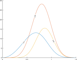
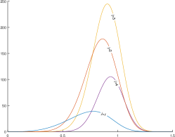
For dimension , the expectation can be computed explicitly, and the resulting numerical values for are given in Table 1.
Recall that the lower incomplete Gamma function is defined as . Its better known complete version, , evaluates to for every positive integer . For half-integers, we have . The -dimensional volume of the unit ball in is , and the -dimensional volume of its boundary is .
Let us make Theorem 1.1 more precise by introducing some notation. The centers of the circumballs of the simplices form a point process in , which in general is not simple. Yet if we restrict this to the centers of intervals — and thus merge the centers of the circumballs of all its simplices into one — we obtain a simple point process. The expected number of centers of intervals in a region is the intensity measure of the interval process. Since the underlying Poisson point process is translation invariant, so is the intensity measure. This shows that the expected number of intervals with , , , and center in factorizes into , with some constant called the intensity of the interval process, and where is an increasing function with . Hence, is a probability distribution function, and we call the distribution of the radius of a typical interval. Theorem 1.1 shows that the radius of the typical interval is Gamma distributed. Clearly, the expected total number of intervals in the Poisson–Delaunay mosaic with center in is . More interestingly, the centers of the circumballs of the -dimensional simplices in the Poisson–Delaunay mosaic in is again a point process. Its intensity is
| (6) |
which can be evaluated explicitly for ; see Table 2. This extends the result of Miles mentioned in [25] to . By Theorem 1.1, we can also get the expected number of simplices with circumradius at most and center in . This seems to be one of the rare examples in the theory of random complexes, in which the precise distribution can be computed.
Corollary 1.2 (Delaunay Simplices).
Let be sampled from a Poisson point process with density in . The expected number of -dimensional simplices of the Poisson–Delaunay mosaic with circumradius at most and center in is
| (7) |
Hence, the distribution of the circumradius of the typical -dimensional simplex is a mixed Gamma distribution:
| (8) |
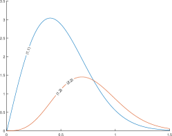
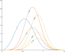
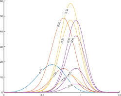
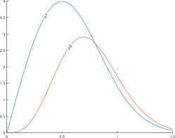
For dimension , the constants can be computed explicitly, with values given in Table 2; see also Figure 1.
As an application we obtain that the expected number of -dimensional simplices in the Delaunay complex for radius with center in is given by (7). For , this is a consequence of the Complementary Theorem due to Miles [22], and we mention the close relation to Gamma type results by Baumstark and Last [2] and Chenavier [7]. It should also be pointed out that Corollary 1.2 can be converted to results for the dual tessellation, the Poisson–Voronoi tessellation. Then (7) gives the intensity of the -dimensional face process of the Poisson–Voronoi tessellation, and (8) the distance of the typical -face to the closest point of the Poisson point process.
The main technical tool used to prove Theorem 1.1 is a Blaschke–Petkantschin type formula that integrates over spheres. Let , write for the Grassmannian consisting of all -planes passing through the origin in , let be the -dimensional unit sphere inside , let be a sequence of points, and write for the -dimensional volume of the -simplex spanned by the . Then for every non-negative function on points, we have
| (9) |
This equation generalizes Theorem 7.3.1 in [25, page 287] to .
While Theorem 1.1 makes a statement about expectations in a fixed region , a standard ergodic argument implies that for a sequence of regions covering the entire space, the numbers of intervals inside , normalized by , converge to the corresponding constants almost surely as random variables, see [20] for details.
Outline. Section 2 introduces the background on discrete Morse theory and Poisson–Delaunay mosaics. Section 3 explains the essential integral geometric tools used to prove Theorem 1.1. Section 4 presents combinatorial and probabilistic results on inscribed simplices. Section 5 uses these results to compute the constants given in Tables 1 and 2. Section 6 concludes the paper.
2. Poisson–Delaunay Complexes
In this section, we introduce the necessary background on Poisson point processes and the radius function on Delaunay mosaics.
Poisson point processes. We study properties of randomly generated discrete point sets in using a Poisson point process with density , which can be characterized by the following two properties:
-
1.
The numbers of points sampled within a finite collection of pairwise disjoint Borel sets are independent random variables;
-
2.
The expected number of points sampled within a Borel set is times the Lebesgue measure of the set.
See [18] for a good introduction to Poisson point processes. Writing for the set sampled from the process, we can express Condition 2 more succinctly as . The two conditions imply that the number of points sampled in a Borel set has a Poisson distribution with parameter . In particular, the probability of having no point in is . Another property that will be important in this paper is the following.
Lemma 2.1 (General Position).
Let be sampled from a Poisson point process in . With probability , is a countable set of points such that for every ,
-
1.
no points belong to a common -plane,
-
2.
no points belong to a common -sphere,
-
3.
considering the unique -sphere that passes through points, no of these points belong to a -plane that passes through the center of the -sphere.
It is not difficult to prove the above lemma, and we refer to [20] and [25] for further information. We say that is in general position if it satisfies the conditions stated in Lemma 2.1. Since it happens with probability , we will assume that is in general position throughout this paper.
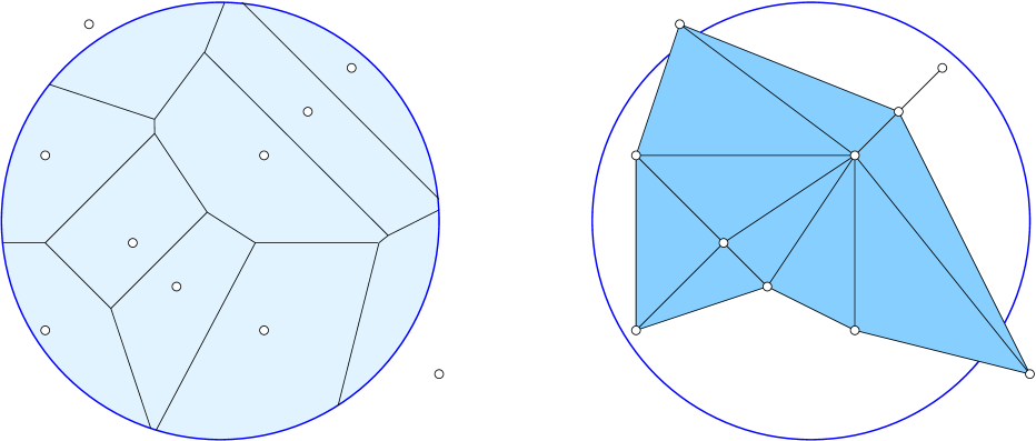
Radius function on Delaunay mosaic. The Voronoi domain of a point consists of all points for which minimizes the Euclidean distance: . With probability , every Voronoi domain is a bounded convex polyhedron [25]. The Voronoi diagram is the collection of Voronoi domains, and the Delaunay mosaic is the nerve of the Voronoi domains; that is: the collection of simplices with non-empty common intersection of Voronoi domains, . The Delaunay mosaic is a simplicial complex iff the Voronoi diagram is primitive, that is: the intersection of any Voronoi domains is either empty or -dimensional. In particular, the intersection of any domains is necessarily empty. Since is in general position with probability , the Voronoi diagram is primitive with probability , and the Delaunay mosaic is a simplicial complex, again with probability .
By construction, every point is equally far from all points in and at least as far from all points in . We call the sphere with center and radius , , a circumsphere because all points of lie on the sphere, and we call it empty because all points of lie on or outside the sphere. The radius function, , maps every simplex to the smallest radius of all its empty circumspheres. As proved in [1], the radius function satisfies the conditions of a generalized discrete Morse function. We refer to [14] for an introduction to discrete Morse theory and to [15] for the generalization needed here. Aiming at a geometric characterization of the intervals, we note that every simplex has a unique smallest circumsphere, namely the unique circumsphere whose center, , lies in the affine hull of . This circumsphere may or may not be empty. Writing in terms of barycentric coordinates, with , we note that the are unique and assuming general position they are also non-zero. Interpreting the barycentric coordinates geometrically, we note that iff the facet is visible from ; that is: there is a ray emanating from that first intersects the interior of the facet before it intersects the interior of the -simplex.
Lemma 2.2 (Geometric Characterization of Intervals).
Letting be in general position, a pair of simplices in defines an interval of iff the smallest circumsphere of is empty and is the largest face of common to all facets that are visible from the center of the sphere.
We refer to [1] for a proof of this characterization. Recall the special case of a critical simplex, , which is characterized by containing inside the convex hull. In this case, the smallest circumsphere is also the smallest sphere that encloses .
Euler characteristic. Letting be a finite subset of , we write for the number of -simplices, for . The sum of these numbers is the size and the alternating sum is the Euler characteristic: and . Importantly, if is a complex, then the Euler characteristic is determined by its homotopy type. For example, if is contractible, then . Now suppose that is a union of intervals of the radius function, and let be the number of -dimensional critical simplices of restricted to . The discrete version of the Morse Relation asserts that the Euler characteristic is also the alternating sum of the :
Lemma 2.3 (Discrete Morse Relation).
Letting be in general position, and a finite subset of the Delaunay mosaic that is a union of intervals of the radius function, the Euler characteristic satisfies .
Proof 2.4.
Consider an interval , and assume that . For each , the number of -simplices in the interval is the number of subsets of size of . The contribution of the interval to the Euler characteristic is therefore . It follows that the non-singular intervals have no effect on the Euler characteristic, which implies the claimed relation.
Subsets and subcomplexes. Assuming is in general position, we use to specify two subsets of the Delaunay mosaic.
- •
-
•
The subset of consists of all simplices in whose smallest empty circumspheres have the center in . We can construct by removing one simplex at a time from . Each removed simplex changes the Euler characteristic by , which gives
(10) We will work with throughout this paper, in particular Theorem 1.1 is proved for .
is interesting for nice sets: in the appendix we prove that if is a ball, then the difference between the number of simplices in and is . This is so because the simplices in correspond to common intersections of Voronoi domains that touch the boundary of , and there are not too many of them. Together with (10), this property implies ; see Appendix A for details. The proof straightforwardly extends from balls to any region with -boundary. It implies that Theorem 1.1 also holds for for smooth after adding .
Theorem 1.1 has the same constant for any Borel set , so it suffices to obtain them for a ball. We can therefore use the aforementioned relation, , which implies the Euler relation for the constants: . Similarly, we have because of Lemma 2.3. Later we will also use the fact that , which is clear for for balls and hence also always holds for .
3. Integral Geometry
We obtain all our results by combining relations from discrete geometry with equations from integral geometry. This section introduces the latter.
Spherical Blaschke–Petkantschin Formula. In its basic form, the Blaschke–Petkantschin Formula decomposes an integral over into an integral over the Grassmannian, , times an integral over a -plane and its orthogonal -plane. We start with the form given in [21, Equation (27)]:
| (11) |
in which , each is a point in , is the -dimensional volume of the simplex spanned by , and is a non-negative function on points. The -th power of the volume compensates for the biased measure on introduced by the Grassmannian. Using Theorem 7.3.1 in [25, page 287], we expand the innermost integral into
| (12) |
in which is the unit -sphere in , and , with each a point on . Note that , so we get as the final power of the radius. Plugging (12) into (11) and joining the integration over and , we get
| (13) |
which is Equation (9) stated in the Introduction. Not surprisingly, for this is the equation in Theorem 7.3.1 of [25].
Slivnyak–Mecke Formula. In a nutshell, the Slivnyak–Mecke Formula writes the expectation of a random variable of a Poisson point process as an integral over the space on which the process is defined; see [25, page 68]. Motivated by the characterization of intervals in Lemma 2.2, we are interested in the expected number of -simplices with empty smallest circumsphere. Writing for the probability that the smallest circumsphere of the simplex spanned by is empty, we get the expected number of -simplices with empty smallest circumspheres as . This integral is, of course, infinite, but it can be made finite by introducing geometric constraints, which can be either understood as restrictions of the integration domain, or as the corresponding indicator functions as multipliers at . For example, to get the number of critical -simplices, we would multiply with , which we set to if the center of the smallest circumsphere lies inside the -simplex spanned by , and to otherwise. More generally, we define
| (16) |
Similarly, we let be the indicator function that the center of this sphere is in , and we let be the indicator function that this sphere has radius at most . We then get the expected number of -simplices whose smallest circumsphere is empty, whose radius is at most , and whose center lies in such facets are visible as
| (17) |
We refer to (17) as a corollary of the Slivnyak–Mecke Formula. Using the Spherical Blaschke–Petkantschin Formula (13), we will rewrite this integral and absorb the latter two indicator functions by limiting the domain. The indicator functions that distinguish between different numbers of visible facets will remain and require further attention.
Counting intervals. We combine the Spherical Blaschke–Petkantschin Formula (13) with the corollary of the Slivnyak–Mecke Formula (17) to get a general expression for the expected number of intervals. Before following up, we recall that the measure of the Grassmannian is , in which is the -dimensional volume of the unit -sphere. For example, may be identified with the set of normal directions and , half the volume of the -dimensional sphere.
The expression for the expected number of intervals will contain the lower incomplete Gamma function, , as a factor. We prefer to explain how this comes about before stating the formula. Write for the -dimensional volume of the ball with radius in , and note that . Hence,
| (18) |
We use (18) to substitute and get the integral into the form of the Gamma function. Specifically,
| (19) |
in which . With this introduction, we are ready to state and prove the general formula for the expected number of intervals.
Lemma 3.1 (Counting Intervals).
Let be chosen from a Poisson point process with density in . For any and , the expected number of -simplices whose smallest circumsphere is empty, whose radius is at most , and whose center lies in such that facets are visible from the center is
| (20) |
Proof 3.2.
Constants. Note that Lemma 3.1 implies Theorem 1.1. The integral in (20) can be interpreted as a scaled expectation of the volume of a -simplex spanned by points uniformly chosen on the unit sphere . With this in mind, we can split (20) into a monstrous but explicit constant factor and this expectation:
| (25) |
which is over the -multivariate uniform distribution on the sphere, and the factor being
| (26) |
in which we use to derive it from the form in (20). To compute the coefficient for small values of and , it is helpful to recall that the measures of the unit spheres are , , , ; see Table 3.
If we ignore the indicator function, this expectation is the -st moment of the -dimensional volume of a random inscribed -simplex. This allows us to write the number of -simplices that are upper bounds of intervals as
| (27) |
The value of this expectation was computed by Miles. For , this gives the number of top-dimensional Delaunay simplices:
| (28) |
see [21]. Since every -simplex has facets, and every -simplex in belongs to two -simplices, we get . This simple relation is perhaps more subtle than it appears. It relies on Lemma 3.1, which writes the expected number of -simplices in the Poisson–Delaunay mosaic as a constant times – without lower order terms – and on Lemma A.3, which implies that the difference between and is of lower order. In dimension , we thus get
| (29) | ||||
| (30) |
4. Inscribed Simplices
In this section, we study the integral in (20) in more detail, reducing it further to cones from the origin over the facets of the simplex.
Volume decomposition. As before, we write for a sequence of distinct points in or, alternatively, for the implied inscribed -simplex. For each , let be the -simplex obtained by substituting for , and write for its -dimensional volume. Expressing the origin in terms of the points, with , we recall that the facet opposite to is visible from iff . Writing for the sign of the -th barycentric coordinate, we therefore have
| (31) |
The multiplicative group acts on the unit sphere by reflection. This action is naturally extended to the action of on -tuples of points: for any vector , with for , we call the reflection with signature of , and we write for the number of indices with . Importantly, the reflection of a vertex does not affect the volume of any cone. We write for the sum of positive and negative cone volumes. Assuming is contained in the interior of the -simplex , the following lemma shows that it is the signed volume of .
Lemma 4.1 (Volume Decomposition).
Let such that is contained in the interior of the -simplex. Then , for every .
Proof 4.2.
We reflect the vertices one by one to obtain from and argue by induction on . By assumption, no facet of is visible from , so , which settles the base case. Assume without loss of generality that with , and with . By induction, the volume of is , i.e., either or , depending on which of the two expressions is positive. Reflecting either changes the orientation of the inscribed -simplex, or it does not. In case the orientation is changed, the reflection changes the visibility of exactly one facet, namely the one opposite to , and by (31) we get either or . In case the orientation is preserved, the reflection changes the visibility of every facet but one, namely the one opposite to , and again by (31) we get either or . Summing up, in all cases we have .
Visibility. There are several useful consequences of Lemma 4.1, which we now state. For example, for almost every inscribed -simplex, there are precisely two signatures for which the corresponding reflections produce a -simplex that contain the origin. To produce one, we reflect every vertex opposite a facet visible from , and to produce the other, we reflect every vertex opposite a facet that is not visible from . If the first simplex corresponds to , then the second corresponds to , which we refer to as the complementary signature.
Corollary 4.3 (Reflections and Visibility).
Let such that is contained in the interior of the -simplex, and let .
-
1.
After reflecting a subset of the vertices, the visible facets are either the ones opposite to the reflected vertices, or all others. Specifically, if , then there are visible facets, each one opposite a reflected vertex, and if , then there are visible facets, each one opposite a non-reflected vertex.
-
2.
The simplices and are central reflections of each other; in particular, they have the same volume and corresponding facets are visible from .
Fact 1 in Corollary 4.3 is a direct consequence of (31) and Lemma 4.1, and Fact 2 is clear for geometric reasons. The following simple facts will be useful in our computations.
Lemma 4.4 (Visibility of Facets).
Let such that is contained in the interior of the -simplex, and let .
-
1.
The origin, , is contained in the interior of the -simplex iff or .
-
2.
implies and, equivalently, implies .
-
3.
If a set of facets is visible from for , then there is no signature such that the complementary set of facets is visible from for .
-
4.
implies and, equivalently, implies .
Proof 4.5.
By assumption on , the only signatures for which all terms have the same sign are the ones for which or . Fact 1 follows and implies Fact 2.
To see Fact 3, we express using (31), getting a negative coefficient for every visible facet. Nevertheless, the sum of signed cone volumes is positive. If the visibility of all facets could be reversed, (31) would give a negative volume, which is a contradiction. Fact 4 follows: it is possible to see every single facet of the simplex, while seeing none of the others, hence it is impossible to see the complementary facets together from .
Fact 1 of Lemma 4.4 appears already in Wendel [26], who generalized it to compute the probability that all points of a finite set sampled independently and uniformly on a sphere lie inside a hemisphere.
Spherical expectations. We now return to (25). The probability space for it is , in which is the uniform measure on the sphere, and the random variables are just the projections. Note that every inscribed simplex, , corresponds to a unique point configuration obtained by projecting from the sphere to the projective space. Likewise, every -simplex with vertices in corresponds to -simplices inscribed in . It allows us to decompose the probability space as , in which is the uniform measure on the projective space and is the uniform measure on . In other words, we decompose the uniform measure on the sphere as the measure on orbits under the action of times the Haar measure on the group. Write for the expectation taken over the sphere, for the expectation over the projective space and for the expectation over the projective space and the group. We use the probabilistic formalism only locally, to decompose the expectation in (25) further into expectations involving volumes of cones. We recall that the volume of is either or . For each , we write the expectation in (25) as
| (32) | ||||
| (33) | ||||
| (34) | ||||
| (35) | ||||
| (36) |
in which in (36) is an arbitrary signature with . The transition to (33) is possible because for a fixed , is the same for all simplices in an orbit, and the transition to (34) is justified by the first fact in Corollary 4.3. We get (35) by observing that the two sums in (34) are over complementary signatures, and we get (36) because relabeling the vertices does not change the expected volume. We can remove the bar in the last transition again because is the same along the orbits. Combining (25) with (36), we finally get the expected number of intervals of each type in terms of the spherical expectations.
Lemma 4.6 (Reduction to Spherical Expectations).
For every , we have .
Moments. We present results on random simplices and their volumes needed to derive the desired expectations. The first result gives the moments of the cone volumes; see [19, Equation 2.11] and with a minor correction [21, Equation (23)]. Let be independently and uniformly distributed on , and write for the corresponding cone, which is a -simplex. Then for any integer , the expectation of is
| (37) |
Besides these moments, we also need the mixed moments to get our results. At the time of writing, we have these only for pairs of cones. Given , we recall that is the cone obtained by substituting for .
Lemma 4.7 (Pairwise Mixed Moments).
Let be a sequence of independently and uniformly distributed points on . Then for any and integers , the expectation of is
| (38) |
Proof 4.8.
Note that and , in which is the -dimensional volume of the shared facet of and , and are the distances of the points from the hyperplane spanned by the shared facet. For geometric reasons, it is clear that are independent; see [19] for details. Hence, we get
| (39) |
with by (37). The value for given in [19], right before Formula (2.11), is times . Substituting the analogous expression for gives the claimed relation.
We illustrate (37) and (38) by computing and for a selected set of small values of , chosen so the results will be useful in Section 5.
5. Constants
Being done with the general facts, we apply them to give concrete expressions for the expected numbers of intervals of the radius function in dimensions up to four. We will mainly compute expectations by integrations – using Equation (20) and Lemma 4.6 – and rarely resort to the linear relations that connect the expectations.
5.1. Two Dimensions
As a warm-up exercise, we begin with a Poisson point process in . We have and for because all vertices are critical. To compute the remaining constants, we need the spherical expectations given in (36):
| (40) |
in which we get the right-hand side because expectations do not change under re-indexing. The expectation is with respect to the uniform distribution on , which is a pair of points. We have and therefore . We also need
| (41) | ||||
| (42) |
which both satisfy , as did (40), so Lemma 4.4 applies and we can remove the indications, which we did. These two expectations are with respect to the uniform distribution on . Using (37) to compute , we get , and similarly . Retrieving and from Table 4, we can now use Lemma 4.6 to get the corresponding constants:
| (43) | ||||
| (44) | ||||
| (45) |
This justifies the entries of the left matrix in Table 1. Note that , which agrees with the discrete Morse relation stated as Lemma 2.3. Indeed, it makes sense to use this relation as a check of correctness as we have refrained from using it during the derivation of the constants.
Remark. As pointed out by Günter Rote, the computations for the critical edges generalize to dimensions. Indeed, and , which gives
| (46) |
Simplices in the Poisson–Delaunay mosaic. For completeness, we also compute the expected numbers of simplices in the -dimensional Poisson–Delaunay mosaic, which are of course known:
| (47) | ||||
| (48) | ||||
| (49) |
We have , which is consistent with the Euler relation in the plane. Note that (45) and (49) imply that about half the Delaunay triangles are critical. The geometric reason behind this fact is an observation by Miles [20] that a Delaunay triangle is acute with probability .
5.2. Three Dimensions
We have and for because every vertex is critical, and we know for the critical edges from (46). To compute the remaining constants in , we need some spherical expectations:
| (50) | ||||
| (51) |
in which the expectations are with respect to the uniform distribution on the circle. We get from (37) and from (38); see also Table 4. Using again Lemma 4.4 to omit indicators, we furthermore have
| (52) | ||||
| (53) |
in which the expectations are with respect to the uniform distribution on the -dimensional sphere. For the moment we skip the computation of . We get from (37). Multiplying the spherical expectation with the corresponding factors in Lemma 4.6, we get the corresponding entries of the middle matrix in Table 1:
| (54) | ||||
| (55) | ||||
| (56) | ||||
| (57) |
We can compute the remaining either by Euler formula or from (27), which gives the constant in the number of -simplices in the Poisson–Delaunay mosaic as ; see also [25]. This gives
| (58) |
which completes the justification of the entries of the middle matrix in Table 1. We use Lemma 2.3 to check the numbers of critical simplices and get , as required.
Simplices in the Poisson–Delaunay mosaic. While the expected numbers of simplices in the Poisson–Delaunay mosaic in are known [25], it is easy to compute them from the above constants:
| (59) | ||||
| (60) | ||||
| (61) | ||||
| (62) |
This completes the entries in the second row of Table 2. As a final check of correctness, we compute the alternating sum, which gives , as required.
5.3. Four Dimensions
In four dimensions, we compute most of the constants directly, but use knowledge of and to get and . We have and for because every vertex is critical, and by (46), so we proceed to the remaining constants.
Triangles as upper bounds. Here we count the critical triangles and edge-triangle pairs. Starting with , we have reflection, and by Lemma 4.4 this implies . We therefore get
| (63) | ||||
| (64) | ||||
| (65) |
From (37) and (38) we get and . Note that and are independent in two dimensions, so we also have , which gives the same result. For the remaining term, we need a convenient description of the three points uniformly chosen on the unit circle. Fixing , we parametrize and by the angles they form with . In this setup, we have , , , where and are uniformly distributed over . We notice that this also implies that and are independent whenever . The moment can now be computed as
| (66) | ||||
| (67) | ||||
| (68) |
in which (68) is true because the expression does not change under transformations and . Computing the integral either by splitting cases or using any mathematical software, we see that the moment evaluates to . Next, we proceed to the critical triangles, computing . For this, we need
| (69) |
Plugging these results into Lemma 4.6, we get
| (70) | ||||
| (71) |
Tetrahedra as upper bounds. Here we count the critical tetrahedra, triangle-tetrahedron pairs, and edge-tetrahedron quadruplets. Starting with , we need the second moment of the volumes of cones with two visible facets. Setting and recalling that , we get
| (72) | ||||
| (73) | ||||
| (74) | ||||
| (75) | ||||
| (76) |
We get from (37), and from (38). Moving on to and to , we need
| (77) | ||||
| (78) |
Plugging these results into Lemma 4.6, we get
| (79) | ||||
| (80) | ||||
| (81) |
-simplices as upper bounds. Here we count the critical -simplices and the intervals they form with tetrahedra, triangles, and edges as lower bounds. For and , we need
| (82) | ||||
| (83) |
We get from (37), and using Lemma 4.6, we get
| (84) | ||||
| (85) |
To avoid the complications that arise from having more than one reflection, we compute and using the linear relations connecting the Delaunay simplices with the intervals. In particular, we get the number of tetrahedra and -simplices in the Poisson–Delaunay mosaic from the intervals as mentioned in Section 1; see also (91) and (92). Since all constants other than the two sought after ones are known, either from the above calculations or from (29) and (30), this leads to a system of two linear equations: and . Solving them, we get
| (86) | ||||
| (87) |
We use Lemma 2.3 to check the number of critical simplices and get , as required.
Simplices in the Poisson–Delaunay mosaic. Finally, we count the simplices in the Poisson–Delaunay mosaic. Using the linear relations that connect the Delaunay simplices with the intervals, we get
| (88) | ||||
| (89) | ||||
| (90) | ||||
| (91) | ||||
| (92) |
This completes the justification of the numbers in Tables 1 and 2. We note that we did not use the Euler Relations to derive any of the constants. We can therefore use it to check whether the computations are possibly correct. Indeed, we get , as required.
6. Discussion
Using a Poisson point process to sample a random set of points in , we study the radius function on the Poisson–Delaunay mosaic [1]. Our main result are integral expressions for the expected numbers of critical simplices and intervals of this generalized discrete Morse function that depend on the maximum allowed radius. This work suggests a number of open questions.
-
1.
We have concrete expressions for the constants that show up in the expectations in dimensions . With the exception of dimensions [25], even the expected numbers of simplices in the Poisson–Delaunay mosaic are currently not known beyond four dimensions. What is the asymptotic behavior of the constants and as goes to infinity?
-
2.
Can the results be extended to weighted Delaunay mosaic as defined in [10]? We suggest that a natural model of such a mosaic is the nerve of an affine slice of a Poisson-Voronoi diagram in . Observe however that the implied distribution of the radii depends on the co-dimension of the slice.
-
3.
Can the results be extended to the Betti numbers and the framework of persistent homology; see e.g. [4]? Indeed, the intervals of size larger than correspond to -persistent pairs, and it is natural to ask similar questions about the pairs with positive persistence.
We finally mention that it is interesting to ask the same questions for the Čech complexes of a Poisson point process in . Mapping each simplex to the radius of the smallest enclosing sphere, we get again a generalized discrete Morse function; see [1]. The critical simplices are the same as for the radius function of the Poisson–Delaunay mosaic, but there is a much richer structure of intervals, which can be analyzed with the methods of this paper.
References
- [1] U. Bauer and H. Edelsbrunner. The Morse theory of Čech and Delaunay complexes. Trans. Amer. Math. Soc., to appear.
- [2] V. Baumstark and G. Last. Gamma distributions for stationary Poisson flat processes. Adv. Appl. Prob. 41 (2009), 911–939.
- [3] O. Bobrowski and R. Adler. Distance functions, critical points, and topology for some random complexes. Homology, Homotopy and Applications 16 (2014), 311–344.
- [4] O. Bobrowski, M. Kahle and P. Skraba. Maximally persistent cycles in random geometric complexes. arXiv:1509.04347, 2015.
- [5] O. Bobrowski and S. Weinberger. On the vanishing of homology in random Čech complexes. arXiv:1507.06945v1, 2015.
- [6] G. Carlsson. Topology and data. Bull. Amer. Math. 46 (2009), 255–308.
- [7] N. Chenavier. A general study of extremes of stationary tessellations with applications. Stoch. Process. Appl. 124 (2014), 2917–2953.
- [8] L. Decreusefond, E. Ferraz, H. Randriam and A. Vergne. Simplicial homology of random configurations. Adv. Appl. Prob. 46 (2014), 1–23.
- [9] T.K. Dey. Curve and Surface Reconstruction. Algorithms with Mathematical Analysis. Cambridge Univ. Press, Cambridge, England, 2011.
- [10] H. Edelsbrunner. Geometry and Topology for Mesh Generation. Cambridge Univ. Press, Cambridge, England, 2001.
- [11] H. Edelsbrunner. Surface reconstruction by wrapping finite sets of points in space. Discrete and Computational Geometry. The Goodman-Pollack Festschrift, 379–404, eds. B. Aronov, S. Basu, J. Pack and M. Sharir, Springer-Verlag, 2003.
- [12] H. Edelsbrunner and J.L. Harer. Computational Topology. An Introduction. Amer. Math. Soc., Providence, Rhode Island, 2010.
- [13] H. Edelsbrunner and E.P. Mücke. Three-dimensional alpha shapes. ACM Trans. Graphics 13 (1994), 43–72.
- [14] R. Forman. Morse theory for cell complexes. Adv. Math. 134 (1998), 90–145.
- [15] R. Freij. Equivariant discrete Morse theory. Discrete Math. 309 (2009), 3821–3829.
- [16] M. Kahle. Random geometric complexes. Discrete Comput. Geom. 45 (2011), 553–573.
- [17] M. Kahle. Topology of random simplicial complexes: a survey. AMS Contemp. Math. 620 (2014), 201–222.
- [18] J.F.C. Kingman. Poisson Processes. Oxford Univ. Press, Oxford, England, 1993.
- [19] R.E. Miles. Poisson flats in Euclidean spaces. Part I: a finite number of random uniform flats. Adv. Appl. Prob. 1 (1969), 211–237.
- [20] R.E. Miles. On the homogeneous planar Poisson point process. Math. Biosci. 6 (1970), 85–127.
- [21] R.E. Miles. Isotropic random simplices. Adv. Appl. Prob. 3 (1971), 353–382.
- [22] R.E. Miles. A synopsis of ‘Poisson flats in Euclidean spaces’. In Stochastic Geometry, eds.: E.F. Harding and D.G. Kendall, John Wiley, New York, 202–227, 1974.
- [23] J. Møller. Random tessellations in . Adv. Appl. Prob. 21 (1989), 37–73.
- [24] F.W.J. Olver. Asymptotics and Special Functions. A.K. Peters, Wellesley, Massachusetts, 1997.
- [25] R. Schneider and W. Weil. Stochastic and Integral Geometry. Springer, Berlin, Germany, 2008.
- [26] J.G. Wendel. A problem in geometric probability. Math. Scand. 11 (1962), 109–111.
Appendix A Boundary Effect
Recall that is the nerve of the Voronoi diagram restricted to , and contains all Delaunay simplices whose smallest empty circumspheres have the center inside . In this appendix, we show that the difference between and is small when is a ball.
Big spheres. We need an auxiliary lemma implying that only a vanishing fraction of the -simplices in the Poisson–Delaunay mosaic have circumspheres with radii larger than some positive threshold. To simplify the discussion, we call the closed ball bounded by the circumsphere of an -simplex its circumball. Letting be bounded and , we write for the number of -simplices in the Poisson–Delaunay mosaic whose circumspheres have the center in and the radius exceeding .
Lemma A.1 (Big Spheres).
There exist positive constants , all depending only on , such that for any bounded Borel region and any fixed , .
Proof A.2.
Size of boundary. We are now ready to give an upper bound on the number of simplices in that are not in , which we need for bound (10) on the Euler characteristic of . Every simplex corresponds to an intersection of Voronoi domains, , that has points inside as well as outside . Let and . We argue that both points are contained in the union of circumballs of the -simplices that share . Indeed, all these circumballs contain all points of , and for each there is a vertex of that is closer to than to , so the circumball centered at this vertex contains . The same argument applies to . Since the union contains points on both sides of , at least one of these circumballs has a non-empty intersection with .
Writing for the number of -simplices whose circumballs have a non-empty intersection with , we prove that it grows slower than the number of -simplices whose circumballs are centered inside . The discussion above implies that , so to have , it is enough to prove the following.
Lemma A.3 (Boundary Size).
Let be a Poisson point process with density in . Let be a ball of radius centered at the origin. Then .
Proof A.4.
Without loss of generality assume . It suffices to count the -simplices with circumcenters outside and to prove that the number of such -simplices whose circumballs intersect is . Assume , fix and let be the set of points at distance at most from . For a ball with center outside to intersect , one of the following must happen:
-
1.
;
-
2.
and its radius exceeds ;
-
3.
and its radius exceeds .
As proved in [25] and reproved in this paper, the expected number of -simplices in with center in is . This settles Case 1. Applying Lemma A.1, we see that the expected number of -simplices with center in and radius larger than is , in which and are positive constants. This settles Case 2. Finally, we decompose the complement of into annuli of the form , for . To intersect , a ball centered inside must have radius exceeding . Writing for the union of annuli and for the number of -simplices with circumcenter in whose circumball intersects , we get an upper bound on the expected number:
| (94) | ||||
| (95) | ||||
| (96) |
where we use Lemma A.1 to get (95), and as well as to get (96). Since the last sum converges, we get , which settles Case 3.
Remarks. Besides , Lemma A.3 implies that the number of vertices of outside is .
Actually, we have proved that for any , . Also, one can apply the Markov’s inequality to show that the convergence happens in probability.