Electron dynamics in graphene with spin-orbit couplings and periodic potentials

Abstract

We use both continuum and lattice models to study the energy-momentum dispersion and the dynamics of a wave packet for an electron moving in graphene in the presence of spin-orbit couplings and either a single potential barrier or a periodic array of potential barriers. Both Kane-Mele and Rashba spin-orbit couplings are considered. A number of special things occur when the Kane-Mele and Rashba couplings are equal in magnitude. In the absence of a potential, the dispersion then consists of both massless Dirac and massive Dirac states. A periodic potential is known to generate additional Dirac points; we show that spin-orbit couplings generally open gaps at all those points, but if the two spin-orbit couplings are equal, some of the Dirac points remain gapless. We show that the massless and massive states respond differently to a potential barrier; the massless states transmit perfectly through the barrier at normal incidence while the massive states reflect from it. In the presence of a single potential barrier, we show that there are states localized along the barrier. Finally, we study the time evolution of a wave packet in the presence of a periodic potential. We discover special points in momentum space where there is almost no spreading of a wave packet; there are six such points in graphene when the spin-orbit couplings are absent.

I Introduction

Graphene has been the arena for an enormous amount of experimental and theoretical research for several years been08 ; neto09 ; rev3 ; rev4 ; rev5 . Graphene consists of a two-dimensional hexagonal lattice of $sp^{2}$ hybridized carbon atoms in which the $\pi$ electrons hop between nearest neighbors. The energy spectrum is gapless at two points in the Brillouin zone; these points are labeled as $K$ and $K^{\prime}$ (this is called the valley degree of freedom), and the energy-momentum dispersion around those points has the Dirac form $E_{{\vec{k}}}=\hbar v|{\vec{k}}|$, where $v\simeq 10^{6}~{}m/s$ is the Fermi velocity. The Dirac nature of the electrons is responsible for many interesting properties of graphene, such as the quantum Hall effect novoselov05 ; zhang05 , Klein tunneling through a barrier katsnelson06 , effects of crossed electric and magnetic fields lukose07 , unusual transport properties of superconducting graphene junctions beenakker1 ; bhattacharjee06 ; bhattacharjee07 ; beenakker2 ; maiti07 , multichannel Kondo physics ksen3 ; kond1 ; kond2 ; kond3 ; kond4 , interesting power laws in the local density of states near an impurity cheianov06 ; mariani07 ; bena08 ; bena09 , and atomic collapse in the presence of charged impurities levitov07 ; wang13 . The effects of Kane-Mele and Rashba spin-orbit (SO) interactions kane1 ; kane2 ; rashba ; zarea09 ; bena14 on the impurity-induced local density of states and on transport across barriers have been examined seshadri1 , and the effect of Rashba SO couplings on tunneling through $pn$ and $pnp$ junctions has been studied liu12 . SO couplings may be induced in graphene in various ways, such as a transverse electric field gmitra09 , adatom deposition weeks11 , or proximity to a three-dimensional topological insulator such as $\rm Bi_{2}Se_{3}$ kou13 ; zhang14 , or functionalizing with methyl zollner15 . (We note that the Kane-Mele and Rashba SO couplings are respectively referred to as intrinsic and extrinsic SO couplings in the literature; however, in this paper we will refer to them as Kane-Mele and Rashba couplings for convenience). The dynamics of wave packets in graphene has been studied in a number of papers using both the microscopic lattice model of graphene costa and a continuum theory which is valid close to the Dirac points maksi ; singh14 ; singh15 .

Recently it has been analytically shown that applying a potential in graphene which is periodic in one or both coordinates can produce additional Dirac points park ; brey ; barbier2 ; barbier3 ; experimental evidence for this in transport measurements has been presented in Ref. dubey, although an alternative explanation has been proposed in Ref. drienovsky, . On the other hand, a potential which is independent of one coordinate and is a random function of the other coordinate is known to give rise to supercollimation, namely, a wave packet moves only in the direction in which the potential varies randomly choi .

In this paper, we study the energy dispersion and wave packet dynamics in graphene in the presence of a periodic potential and SO couplings. The plan of the paper is as follows. In Sec. II, we use a continuum theory near the Dirac points (labeled $K$ and $K^{\prime}$) to study the energy dispersion in the presence of SO couplings and a periodic array of $\delta$-function potentials. In the absence of a periodic potential, a Kane-Mele SO coupling produces a gap at the Dirac points which is doubly degenerate (for a given momentum) due to the spin and valley degrees of freedom. A combination of Kane-Mele and Rashba SO couplings produces four non-degenerate states. When the two SO couplings are equal, two of the states have a gapless Dirac form while the other two have a gapped Dirac form. The presence of a periodic potential generates additional Dirac points as known in the literature; we show that spin-orbit couplings generally open gaps at those points unless the two couplings are equal. (A related study was carried out in Ref. shakouri, ). In Sec. III, we use the microscopic lattice model of graphene to study the energy dispersion in the presence of SO couplings and a single potential barrier. This confirms the results obtained using continuum theory in Sec. II. In addition, we show that there are states which are localized along the barrier and whose energies lie in the bulk gap seshadri2 . In Sec. IV, we use the lattice model to study wave packet dynamics in the presence of a periodic potential and SO couplings. The wave packets are be taken to be Gaussians. For graphene without any SO couplings, we analytically find six special points in the Brillouin zone where there is negligible spreading of a wave packet. When the Kane-Mele and Rashba SO couplings are non-zero but equal, we show that wave packets constructed from the two kinds of states (the gapless Dirac and the gapped Dirac states discussed in Sec. II) respond quite differently to the barriers. We conclude in Sec. V with a summary of our main results.

II Continuum theory around Dirac points

In this section, we will use a continuum theory around the Dirac points (which lie at two momenta called $K$ and $K^{\prime}$) to study the energy spectrum in the presence of SO couplings and a potential which is periodic in one direction. We will consider both a Kane-Mele SO coupling kane1 ; kane2 called $\Delta_{KM}$ and a Rashba SO coupling rashba ; zarea09 ; bena14 called $\lambda_{R}$. Further, a periodic potential which only depends on the $y$-coordinate is applied; the precise form of this potential will be specified below, and we will assume that it has the symmetry $V(y)=V(-y)$. Since the system has translational symmetry along the $x$ direction, the momentum $k_{x}$ along this direction is a good quantum number. The complete Hamiltonian close to the Dirac points is then given by

$$H = \hbar v_{F}(\tau^{z}\sigma^{x}k_{x}+i\sigma^{y}\frac{\partial}{\partial y})~{}+~{}\Delta_{KM}\tau^{z}\sigma^{z}s^{z}$$ (1)

$$+~{}\lambda_{R}(\tau^{z}\sigma^{x}s^{y}-\sigma^{y}s^{x})~{}+~{}V(y),$$

where $\sigma^{a}$, $\tau^{a}$ and $s^{a}$ are Pauli matrices corresponding to sublattice ($\sigma^{z}=+(-)~{}1$ for $A(B)$), valley ($\tau^{z}=+(-)~{}1$ for $K(K^{\prime})$) and spin ($s^{z}=+(-)~{}1$ for up (down) spin) respectively. The Fermi velocity $v_{F}\simeq 10^{6}~{}m/s$ and $k_{x}$ is the deviation from the Dirac point. (Henceforth we will set $\hbar=1$ unless otherwise mentioned).

We first look at the various symmetries of the Hamiltonian in Eq. (1); these will imply certain symmetries of the energy spectrum and eigenstates.

1. For a given value of $\tau^{z}$, we have

$$H(k_{x},y,\tau^{z})~{}=~{}\sigma^{x}s^{y}~{}H(k_{x},-y,\tau^{z})~{}\sigma^{x}s^{y}.$$ (2)

2. The Hamiltonians at $K$ and $K^{\prime}$ are related by

$$H(k_{x},y,\tau^{z})~{}=~{}\tau^{x}\sigma^{x}s^{z}~{}H(k_{x},-y,-\tau^{z})~{}\tau^{x}\sigma^{x}s^{z}.$$ (3)

3. $\tau^{x}\sigma^{y}$, $\tau^{y}\sigma^{y}$ and $\tau^{z}$ all commute with $H$ and anticommute with one another. As a result, the $\tau^{z}=\pm 1$ sectors are degenerate.

4. If $\lambda_{R}=0$, the Hamiltonian has the symmetry

$$H(k_{x},y,\tau^{z})=\sigma^{x}s^{x}~{}H(k_{x},-y,\tau^{z})~{}\sigma^{x}s^{x}.$$ (4)

5. For a given value of $\tau^{z}$, the Hamiltonian has the symmetry

$$H(k_{x},y,\tau^{z})=\sigma^{y}s^{x}~{}H(-k_{x},y,\tau^{z})~{}\sigma^{y}s^{x}.$$ (5)

This implies that the energy spectrum is invariant under $k_{x}\to-k_{x}$.

We observe that the symmetries in Eqs. (2) and (3) flip the spin $s^{z}\to-s^{z}$; we therefore get a double degeneracy of all energy levels due to spin.

At the Dirac point $K$, i.e. $\tau^{z}=+1$, Eq. (1) reduces to a $4\times 4$ matrix given by

$$H = v_{F}(\sigma^{x}k_{x}+i\sigma^{y}\frac{\partial}{\partial y})~{}+~{}\Delta_{KM}\sigma^{z}s^{z}$$ (6)

$$+~{}\lambda_{R}(\sigma^{x}s^{y}-\sigma^{y}s^{x})~{}+~{}V(y).$$

For a periodic potential satisfying $V(y)=V(y+d)$, the eigenstates can be labeled by a Bloch momentum $\chi_{y}$ (which lies in the range $[-\pi/d,\pi/d]$), namely, $\psi(k_{x},y+d)=e^{i\chi_{y}d}\psi(k_{x},y)$. The symmetry $\sigma^{x}s^{y}H(k_{x},-y)\sigma^{x}s^{y}=H(k_{x},y)$ then implies that the spectrum is symmetric about $\chi_{y}=0$ for all $k_{x}$.

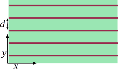
Figure 1: Schematic diagram of a $\delta$-function potential which repeats periodically in the $y$ direction with a spacing $d$.

We will numerically compute the energy spectrum for a periodic $\delta$-function potential which is independent of the $x$ coordinate, i.e.,

$$V(x,y)~{}=~{}C~{}\sum_{n=-\infty}^{\infty}\delta(y-nd),$$ (7)

where $C$ is the strength of the $\delta$-function. ($C$ has the dimensions of energy times length). The unit cell size of the periodic potential in the $y$ direction is $d$. A schematic picture of the periodic potential is shown in Fig. 1.

One way of studying the effect of a $\delta$-function potential in a Dirac Hamiltonian is to note that it induces a discontinuity in the wave function of the form $\psi(x,y=d+)=\exp[i(C/\hbar v_{F})\sigma^{y}]\psi(x,y=d-)$ for a $\delta$-function of strength $C$ located at $y=d$. deb12 Using this along with the Bloch theorem which states that $\psi(x,y=d+)=\exp(i\chi_{y}d)\psi(x,y=0+)$, where $\chi_{y}$ is the Bloch momentum, we can reduce the problem of finding the energies and eigenstates as a function of $k_{x}$ and $\chi_{y}$ to solving a differential equation within a single unit cell of the periodic potential. Namely, if we write $\psi(x,y)=e^{ik_{x}x}f(y)$, then the four-component spinor $f(y)$ must satisfy

$$[v_{F}(\sigma^{x}k_{x}+i\sigma^{y}\frac{\partial}{\partial y})~{}+~{}\Delta_{KM}\sigma^{z}s^{z}$$

$$+~{}\lambda_{R}(\sigma^{x}s^{y}-\sigma^{y}s^{x})]~{}f~{}=~{}E~{}f$$ (8)

in the region $0<y<d$, subject to the boundary condition $e^{i\chi_{y}d}f(0+)=e^{i(C/\hbar v_{F})\sigma^{y}}f(d-)$. However we found that this method is numerically not convenient for finding the energy dispersion.

We have therefore used a different numerical method for finding the dispersion. Given a value of $k_{x}$ and $\chi_{y}$, the general wave function consistent with the Bloch theorem is given by

$$\psi(x,y)=e^{ik_{x}x}~{}\sum_{m=-\infty}^{\infty}~{}e^{i(\chi_{y}+2\pi m/d)y}f_{m}(y).$$ (9)

Let us truncate the range of $m$ in Eq. (9) to go from $-q$ to $+q$; this gives a total of $2q+1$ bands. The Hamiltonian in this basis is then a $4(2q+1)$- dimensional matrix with blocks of matrix elements as follows. First, there are $2q+1$ blocks on the diagonal which are given by $4\times 4$ matrices of the form

$$v_{F}[\sigma^{x}k_{x}-\sigma^{y}(\chi_{y}+\frac{2\pi m}{d})]+\Delta_{KM}\sigma^{z}s^{z}+\lambda_{R}(\sigma^{x}s^{y}-\sigma^{y}s^{x}).$$ (10)

Second, the identity

$$C\sum_{n=-\infty}^{\infty}~{}\delta(y-nd)~{}=~{}\frac{C}{d}~{}\sum_{m=-\infty}^{\infty}~{}e^{i2\pi my/d},$$ (11)

implies that between any two blocks labeled by $m$ and $m^{\prime}$ (each label runs from $-q$ to $+q$, and $m,~{}m^{\prime}$ may or may not be equal), there will be a coupling given by $(C/d)I_{4}$, where $I_{4}$ is the $4\times 4$ identity matrix. Putting these together we get the total Hamiltonian from which we can obtain $4(2q+1)$ energy levels.

In Fig. 2, we show the energy spectrum $E$ versus the Bloch momentum $\chi_{y}$ (lying in the range $[-\pi/d,\pi/d]$) for $\tau^{z}=1$, $k_{x}=0$ and $d=200$, and various values of the $\delta$-function strength $C$ and SO couplings $\Delta_{KM}$ and $\lambda_{R}$. (In these calculations, we have kept 41 bands, namely, $q=20$. We have checked that the results do not change noticeably if we consider more than 41 bands). To see the effects of the periodic potential clearly, we have shown the spectra without the potential in Figs. 2 (a), (c), (e) and (g), and with the potential in Figs.  2 (b), (d), (f) and (h). Fig. 2 (b) shows that for graphene without any SO couplings ($\Delta_{KM}=\lambda_{R}=0$), additional gapless Dirac points appear at the center ($\chi_{y}=0$) and the ends of the reduced Brillouin zone ($\chi_{y}=\pm\pi/d$) when a periodic potential is present. We can understand the appearance of these gapless Dirac points as follows. For normal incidence on a barrier (i.e., for $k_{x}=0$), a gapless Dirac particle transmits perfectly (this is called Klein tunneling). The absence of reflection implies that the periodic potential does not lead to any mixing between modes with momenta $k_{y}=+m\pi/d$ and $-m\pi/d$. (Recall that a potential with periodicity $d$ can only produce scattering between pairs of states whose $y$-momenta differ by an integer multiple of $2\pi/d$). Hence the energy degeneracy between the modes at $k_{y}=\pm m\pi/d$ remains unbroken, and no gap is produced. Next, Figs. 2 (d) and (f) show the effects of Kane-Mele and Rashba SO couplings separately; we see that these couplings generally open gaps at the additional Dirac points. Finally, Fig. 2 (h) shows that when both SO couplings are present with $\Delta_{KM}=\lambda_{R}$, some of the gapless Dirac points are restored; these gapless points are particularly easy to see at the ends of Brillouin zone ($\chi_{y}=\pm\pi/d$). We will now see why $\Delta_{KM}=\pm\lambda_{R}$ is special.

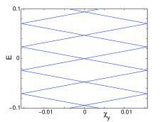
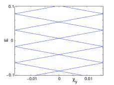
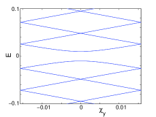
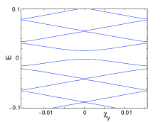
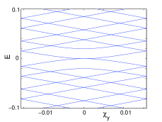
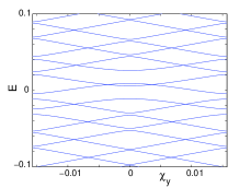
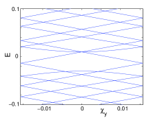
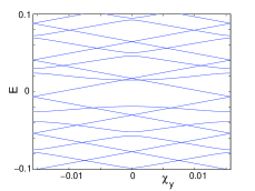
Figure 2: $E$ vs $\chi_{y}$ for $k_{x}=0$ and $d=200$. ($d$ is in units of the lattice spacing, while $E$ is in units of $\gamma$). The figures on the left ((a),(c),(e),(g)) are in the absence of the $\delta$-function periodic potential ($C=0$), while the ones on the right ((b),(d),(f),(h)) are with $C=\pi\gamma/2$ times the lattice spacing. In (a) and (b), $\Delta_{KM}=\lambda_{R}=0$; in (c) and (d), $\Delta_{KM}=0.01~{}\gamma$, $\lambda_{R}=0$; in (e) and (f), $\Delta_{KM}=0$, $\lambda_{R}=0.01~{}\gamma$; in (g) and (h), $\Delta_{KM}=\lambda_{R}=0.01~{}\gamma$.

When the potential $V(y)=0$, the momenta $k_{x}$ and $k_{y}$ are both good quantum numbers. The energy spectrum of the Hamiltonian in Eq. (1) is then given by seshadri1

$$\Big{[}E^{2}~{}-~{}v_{F}^{2}{\vec{k}}^{2}~{}-~{}\Delta_{KM}^{2}\Big{]}^{2}~{}=~{}4\lambda_{R}^{2}~{}(E-\Delta_{KM})^{2},~{}~{}~{}~{}~{}~{}~{}~{}~{}~{}~{}$$ (12)

where ${\vec{k}}^{2}=k^{2}_{x}+k^{2}_{y}$. This can be solved to give four branches of solutions for $E$,

$$E = \lambda_{R}~{}\pm~{}\sqrt{v_{F}^{2}{\vec{k}}^{2}~{}+~{}(\Delta_{KM}-\lambda_{R})^{2}},~{}~{}~{}\text{and}$$

$$E = -\lambda_{R}~{}\pm~{}\sqrt{v_{F}^{2}{\vec{k}}^{2}~{}+~{}(\Delta_{KM}+\lambda_{R})^{2}}.$$ (13)

We therefore see that if $\Delta_{KM}=\pm\lambda_{R}$, the dispersion in the region around $(k_{x},k_{y})=(0,0)$ has the massless Dirac form in two of the branches ($E=\pm v_{F}|\vec{k}|$ plus a constant) and the massive Dirac form in the other two branches ($E=\pm\sqrt{v_{F}^{2}{\vec{k}}^{2}+4\Delta_{KM}^{2}}$ plus a constant). Depending on which branch we consider, we expect two different kinds of behaviors when a periodic potential $V(y)$ is turned on: additional gapless Dirac points and perfect Klein tunneling at normal incidence ($k_{x}=0$) from the massless Dirac branches, and gaps at the additional Dirac points and a non-zero reflection from the massive Dirac branches. This can be shown as follows.

For $k_{x}=0$, Eq. (1) takes the form

$$H = iv_{F}\sigma^{y}\frac{\partial}{\partial y}+\Delta_{KM}\tau^{z}\sigma^{z}s^{z}+\lambda_{R}(\tau^{z}\sigma^{x}s^{y}-\sigma^{y}s^{x})$$ (14)

$$+~{}V(y).$$

This Hamiltonian commutes with $\tau^{z}$ and $\sigma^{y}s^{x}$; we can therefore work in a particular sector of eigenstates of $\tau^{z}$ and $\sigma^{y}s^{x}$ with eigenvalues equal to $+1$ or $-1$. Since $(\tau^{z}\sigma^{z}s^{z})(\tau^{z}\sigma^{x}s^{y})=\sigma^{y}s^{x}$, we see that the combination $\Delta_{KM}\tau^{z}\sigma^{z}s^{z}+\lambda_{R}\tau^{z}\sigma^{x}s^{y}$ vanishes in the sector $\sigma^{y}s^{x}=-1$ if $\Delta_{KM}=\lambda_{R}$ and in the sector $\sigma^{y}s^{x}=+1$ if $\Delta_{KM}=-\lambda_{R}$. In these sectors, therefore, the Hamiltonian in (14) reduces to

$$H~{}=~{}iv_{F}\sigma^{y}\frac{\partial}{\partial y}~{}\pm~{}\lambda_{R}~{}+~{}V(y),$$ (15)

where the $\pm$ signs in front of $\lambda_{R}$ are for the cases $\Delta_{KM}=\pm\lambda_{R}$ respectively; these are the sectors which contain the massless Dirac modes if $k_{x}=0$ and $V(y)=0$. Next, we find that for an arbitrary potential $V(y)$, the eigenstates and spectrum of Eq. (15) are given by

$$\psi_{k_{y},s}(y) = \exp[ik_{y}y+(is/v_{F})\int_{0}^{y}dy^{\prime}V(y^{\prime})]~{}u_{k_{y},s},$$

$$E_{k_{y}} = \pm\lambda_{R}~{}-~{}v_{F}sk_{y},$$ (16)

where the spinor $u_{k_{y},s}$ is an eigenstate of $\sigma^{y}$ with eigenvalue $s=\pm 1$ and an eigenstate of $\sigma^{y}s^{x}$ with eigenvalue $\pm 1$. We thus see that there is perfect transmission through any potential $V(y)$, and the spectrum varies linearly with $k_{y}$. For a periodic potential, the perfect transmission and hence the absence of reflection for the massless Dirac modes implies that the degeneracy between states at $k_{y}=\pm m\pi/d$ remains unbroken, and no gap is produced at the additional Dirac points. In Sec. IV, we will see directly that the massless and massive Dirac states indeed show different transmission and reflection properties.

III Lattice model

In this section we use the microscopic lattice model to study the energy spectrum in the presence of a periodic potential and SO couplings. We will consider the honeycomb lattice shown in Fig. 3 with periodic boundary conditions in both directions. (We will usually set the nearest-neighbor lattice spacing $a=0.142$ nm equal to 1). The zigzag rows run parallel to the $x$ direction. Each unit cell consists of an $a$ site and a $b$ site; the cells are labeled by two integers $(n_{x},n_{y})$ as shown. (The size of a unit cell in the $y$ direction is $3a/2$). Since the system has translational symmetry along the $x$ direction, the momentum $k_{x}$ in that direction is a good quantum number. The plane wave factors depending on $k_{x}$ are shown at the top of Fig. 3.

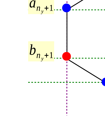
Figure 3: Schematic diagram of the honeycomb lattice used to calculate the spectra shown in Fig. 4. The $x$ coordinate increases from left to right while the $y$ coordinate increases from top to bottom. The plane wave factors shown at the top are dependent on the momentum $k_{x}$. The unit cells are denoted by ellipses and consist of one $a$ site and one $b$ site.

In second quantized notation, the complete Hamiltonian $H$ of the lattice model is the sum of four terms,

$$H_{0} = -\gamma~{}\sum_{\langle ij\rangle,s}~{}f^{\dagger}_{is}f_{js},$$ (17a)

$$H_{KM} = it_{2}~{}\sum_{\langle\langle ij\rangle\rangle,s}~{}\nu_{ij}~{}s^{z}_{ss}f^{\dagger}_{is}f_{js},$$ (17b)

$$H_{R} = i\lambda_{R}~{}\sum_{\langle ij\rangle,ss^{\prime}}~{}\hat{z}\cdot(\vec{d}_{ij}\times\vec{s})_{ss^{\prime}}~{}f^{\dagger}_{is}f_{js^{\prime}},$$ (17c)

$$H_{V} = \sum_{i}~{}V_{i}~{}f^{\dagger}_{i}f_{i},$$ (17d)

$$H = H_{0}~{}+~{}H_{KM}~{}+~{}H_{R}~{}+~{}H_{V},$$ (17e)

where $\langle ij\rangle$ denotes nearest neighbors ($i$ and $j$ are labeled by $n_{x},n_{y}$), $\langle\langle ij\rangle\rangle$ denotes next-nearest neighbors, and the subscripts $s,s^{\prime}$ denote the spin component $s^{z}=\pm 1$. Eqs. (17a), (17b) and (17c) describe graphene without any SO couplings, with Kane-Mele kane1 ; kane2 and with Rashba SO terms respectively rashba ; zarea09 ; bena14 . In (17a), $\gamma\simeq 2.8$  eV denotes the nearest-neighbor hopping amplitude; the Fermi velocity in Sec. II is given by $v_{F}=(3/2)\gamma a$. In (17b), $\nu_{ij}=\pm 1$ depending on the relative orientation of the two successive nearest-neighbor vectors which join site $j$ to its next-nearest-neighbor site $i$. In (17c), $\vec{d}_{ij}$ denotes the vector joining the nearest-neighbor sites $i$ and $j$. In the continuum theory near the Dirac points, Eq. (17b) reduces to the Kane-Mele term in Eq. (1) with $\Delta_{KM}=3\sqrt{3}t_{2}$, while Eq. (17c) reduces to the Rashba term in Eq. (1). Finally, we will take the potential $V_{i}$ in (17d) to be a periodic function of $n_{y}$ and independent of $n_{x}$. More specifically, we will choose the periodic potential $V_{i}$ to be composed of Gaussians, rather than the $\delta$-function potentials that we considered in Sec. II. Namely, we will take

$$V(n_{y})~{}=~{}\frac{C}{\sigma\sqrt{2\pi}}~{}\sum_{n=-\infty}^{\infty}~{}e^{-[(3a/2)n_{y}-nd]^{2}/(2\sigma^{2})},$$ (18)

where $d$ is the periodicity of the potential; in our calculations we have chosen the width of the Gaussians to be $\sigma=4a$.

From the Hamiltonian in Eq. (17e), we can write down the eigenvalue equations for an energy $E$. For a given momentum $k_{x}$ we can effectively reduce the system to a one-dimensional chain which runs along the $y$-direction. The unit cells of the chain are labeled by an integer $n_{y}$; each unit cell has four variables labeled $a_{n_{y}\uparrow},~{}a_{n_{y}\downarrow},~{}b_{n_{y}\uparrow}$ and $b_{n_{y}\downarrow}$. Using the plane wave factors shown in Fig. 3, we find the following equations.

$$E~{}a_{n_{y}\uparrow} = -~{}\gamma~{}\Big{\{}b_{n_{y}\uparrow}~{}+~{}2\cos(\frac{\sqrt{3}k_{x}}{2})b_{n_{y}-1\uparrow}\Big{\}}~{}+~{}2t_{2}~{}\Big{\{}\sin(\sqrt{3}k_{x})a_{n_{y}\uparrow}~{}-~{}\sin(\frac{\sqrt{3}k_{x}}{2})(a_{n_{y}-1\uparrow}~{}+~{}a_{n_{y}+1\uparrow})\Big{\}}$$

$$+~{}i\lambda_{R}~{}\Big{\{}\Big{(}\cos(\frac{\sqrt{3}k_{x}}{2})~{}+~{}\sqrt{3}\sin(\frac{\sqrt{3}k_{x}}{2})\Big{)}b_{n_{y}-1\downarrow}-b_{n_{y}\downarrow}\Big{\}}~{}+~{}V_{n_{y}}~{}a_{n_{y}\uparrow},$$

$$E~{}a_{n_{y}\downarrow} = -~{}\gamma~{}\Big{\{}b_{n_{y}\downarrow}~{}+~{}2\cos(\frac{\sqrt{3}k_{x}}{2})b_{n_{y}-1\downarrow}\Big{\}}~{}-~{}2t_{2}~{}\Big{\{}\sin(\sqrt{3}k_{x})a_{n_{y}\downarrow}~{}-~{}\sin(\frac{\sqrt{3}k_{x}}{2})(a_{n_{y}-1\downarrow}~{}+~{}a_{n_{y}+1\downarrow})\Big{\}}$$

$$+~{}i\lambda_{R}~{}\Big{\{}\Big{(}\cos(\frac{\sqrt{3}k_{x}}{2})~{}-~{}\sqrt{3}\sin(\frac{\sqrt{3}k_{x}}{2})\Big{)}b_{n_{y}-1\uparrow}~{}-~{}b_{n_{y}\uparrow}\Big{\}}~{}+~{}V_{n_{y}}~{}a_{n_{y}\downarrow},$$

$$E~{}b_{n_{y}\uparrow} = -~{}\gamma~{}\Big{\{}a_{n_{y}\uparrow}~{}+~{}2\cos(\frac{\sqrt{3}k_{x}}{2})a_{n_{y}+1\uparrow}\Big{\}}~{}-~{}2t_{2}~{}\Big{\{}\sin(\sqrt{3}k_{x})b_{n_{y}\uparrow}~{}-~{}\sin(\frac{\sqrt{3}k_{x}}{2})(b_{n_{y}-1\uparrow}~{}+~{}b_{n_{y}+1\uparrow})\Big{\}}$$

$$-~{}i\lambda_{R}~{}\Big{\{}\Big{(}\cos(\frac{\sqrt{3}k_{x}}{2})~{}-~{}\sqrt{3}\sin(\frac{\sqrt{3}k_{x}}{2})\Big{)}a_{n_{y}+1\downarrow}~{}-~{}a_{n_{y}\downarrow}\Big{\}}~{}+~{}V_{n_{y}}~{}b_{n_{y}\uparrow},$$

$$E~{}b_{n_{y}\downarrow} = -~{}\gamma~{}\Big{\{}a_{n_{y}\downarrow}~{}+~{}2\cos(\frac{\sqrt{3}k_{x}}{2})a_{n_{y}+1\downarrow}\Big{\}}~{}+~{}2t_{2}~{}\Big{\{}\sin(\sqrt{3}k_{x})b_{n_{y}\downarrow}~{}-~{}\sin(\frac{\sqrt{3}k_{x}}{2})(b_{n_{y}-1\downarrow}~{}+~{}b_{n_{y}+1\downarrow})\Big{\}}$$ (19)

$$-~{}i\lambda_{R}~{}\Big{\{}\Big{(}\cos(\frac{\sqrt{3}k_{x}}{2})~{}+~{}\sqrt{3}\sin(\frac{\sqrt{3}k_{x}}{2})\Big{)}a_{n_{y}+1\uparrow}~{}-~{}a_{n_{y}\uparrow}\Big{\}}~{}+~{}V_{n_{y}}~{}b_{n_{y}\downarrow}.$$

Note that we have absorbed the lattice spacing $a$ into the definition of $k_{x}$ thereby making it a dimensionless quantity. By solving the above equations numerically, we can obtain $E$ as a function of $k_{x}$.

In Fig. 4, we show $E$ versus $k_{x}$ for various cases. (In our calculations, we have taken $N_{y}=200$ unit cells in the $y$-direction. Hence the Hamiltonian is an $800\times 800$ matrix due to the sublattice and spin degrees of freedom. We will also set $\gamma=1$ and the lattice spacing $a=1$). Figs. 4 (a), (b) and (c) show the energy spectrum when there is no potential ($V_{n_{y}}=0$), while Figs. 4 (d), (e) and (f) show the spectrum in the presence of a single potential barrier which has a Gaussian shape. The width of the barrier is $4a$ and its peak value is $C=\gamma/3$, where $\gamma$ is the nearest-neighbor hopping amplitude. Figures 4 (a) and (d) are for graphene without any SO couplings, i.e., $t_{2}=\lambda_{R}=0$. In Figs. 4 (b) and (e), $t_{2}=0.02~{}\gamma$ and $\lambda_{R}=0$, while in Figs. 4 (c) and (f), $t_{2}=\lambda_{R}=0.02~{}\gamma$. The blue shaded regions denote bulk states. The red dashed lines show states which are localized along the barrier; their wave functions decay exponentially as we go away from the barrier but are plane waves along the barrier. These one-dimensional states occur in a variety of systems described by the Dirac equation, such as graphene seshadri2 and surfaces of three-dimensional topological insulators deb12 .

We note that the modes localized along the barrier (shown by red dashed lines in Figs. 4 (d,e,f)) are not topologically protected. The modes in Figs. 4 (d,f) are not topologically protected because the system is gapless and therefore in a non-topological phase on both sides of the barrier. The modes in Fig. 4 (e) are not topologically protected because the system is in the same topological phase on both sides of the barrier.

The states localized along the barrier have an interesting spin and sublattice structure. In Fig. 5, we show the probabilities of $a\uparrow$, $a\downarrow$, $b\uparrow$ and $b\downarrow$ as a function of the unit cell index $n_{y}$ for two states produced by a barrier of width $4a$ and peak value $\gamma/3$; we have taken $t_{2}=0.02~{}\gamma$ and $\lambda_{R}=0$. The two states are degenerate in energy, and we see from the figure that the various probabilities in the two states are related to each other by a simultaneous interchange of sublattice and spin. This symmetry follows from the observation that for $\lambda_{R}=0$, Eqs. (19) are invariant under the interchanges $a_{n_{y}\uparrow}\leftrightarrow b_{-n_{y}\downarrow}$ and $a_{n_{y}\downarrow}\leftrightarrow b_{-n_{y}\uparrow}$, assuming that $V_{n_{y}}=V_{-n_{y}}$. (We note that this is the lattice version of the symmetry of the continuum theory that was pointed out in Eq. (4)).

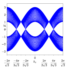
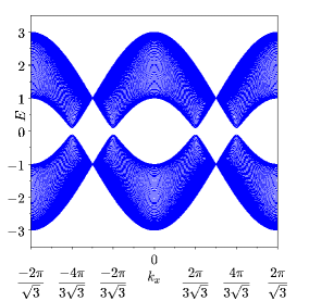
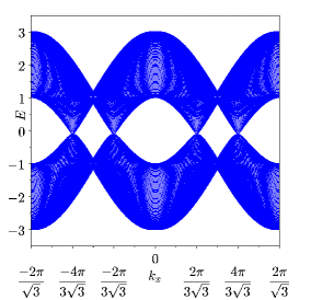
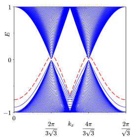
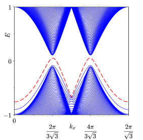
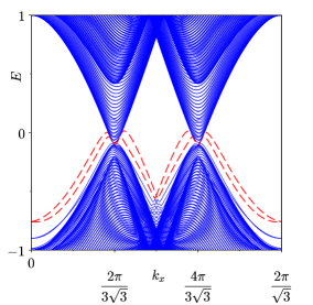
Figure 4: $E$ vs $k_{x}$ for various systems. ($k_{x}$ is in units of $1/a$ while $E$ is in units of $\gamma$). Figures (a,b,c) and (d,e,f) show the spectrum without and with a single potential barrier respectively. The width of the barrier is $4a$ and its peak value is $C=\gamma/3$. In Figs. (a) and (d), $\Delta_{KM}=\lambda_{R}=0$; in Figs. (b) and (e), $\Delta_{KM}=0.1~{}\gamma$ and $\lambda_{R}=0$; in Figs. (c) and (f), $\Delta_{KM}=\lambda_{R}=0.1~{}\gamma$. The blue shaded regions denote bulk states while the red dashed lines in Figs. (d), (e) and (f) show states which are localized along the barrier. In Figs. (d) and (e), the states localized along the barrier are doubly degenerate due to spin; this degeneracy is broken in Fig. (f) due to the Rashba SO coupling.

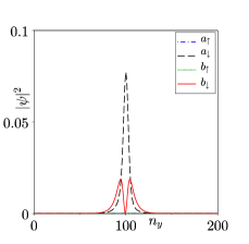
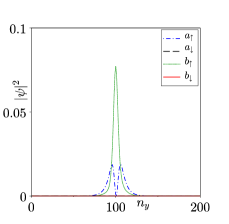
Figure 5: $|\psi|^{2}$ vs $n_{y}$ for two degenerate states localized along a barrier of width $4a$ and peak value $\gamma/3$. The SO couplings are given by $\Delta_{KM}=0.1~{}\gamma$ and $\lambda_{R}=0$. The probabilities on sites $a\uparrow$, $a\downarrow$, $b\uparrow$ and $b\downarrow$ are shown by blue dot dash, black dashed, green dot and red solid lines respectively.

IV Wave packet dynamics

To numerically study the time evolution of a Gaussian wave packet on a honeycomb lattice, we take the rows of zigzag bonds to be parallel to the $x-$axis. Since our system has translational symmetry in the $x$ direction, $k_{x}$ is a good quantum number. However, periodic barriers parallel to the zigzag rows (Fig. 1), break the translational invariance in the $y$ direction. We therefore consider a real space lattice with $N_{y}=360$ unit cells in the $y$-direction. Hence, for every $k_{x}$, the Hamiltonian $H(k_{x})$ is a $4N_{y}\times 4N_{y}$ matrix (accounting for the spin and sublattice degrees of freedom) and has periodic boundary condition in the $y$ direction. We denote the eigenvalues and eigenvectors of $H(k_{x})$ by $E_{k_{x}}^{(n)}$ and $\phi_{k_{x}}^{(n)}$ respectively.

We take the initial wave packet $\Psi(t=0)$ to be a Gaussian constructed such that it has a peak momentum ${\vec{k}}_{0}$, peak position $\vec{r_{0}}$ and width $(W_{x},W_{y})$ of our choice. It is constructed out of the eigenvectors of the $4\times 4$ lattice Hamiltonian $H(k_{x},k_{y})$ that we would get if both $k_{x}$ and $k_{y}$ were good quantum numbers; we choose the eigenvectors to lie within the positive energy band, $E_{k_{x},k_{y}}\geq 0$. The width of the wave packet in momentum space is inversely proportional to the width in real space. Hence a Gaussian which is narrow in real space has a large contribution from momenta far away from ${\vec{k}}_{0}$, while a Gaussian which is wide in real space has contributions only from momenta which lie close to ${\vec{k}}_{0}$.

We incorporate periodic boundary conditions in the $x$ direction by taking $k_{x}$ in integer multiples of $2\pi/(N_{x}\sqrt{3}a)$; we have chosen $N_{x}=312$. We study the evolution of the wave packet by letting each of the momentum components $k_{x}$ evolve independently in time and then superposing them with suitable coefficients to form a Gaussian.

To summarize, let $\phi^{(n)}_{k_{x}}$ denote the $n$-th eigenvector of the $4N_{y}\times 4N_{y}$ Hamiltonian $H(k_{x})$, i.e.,

$$H(k_{x})\phi^{(n)}_{k_{x}}~{}=~{}E^{(n)}_{k_{x}}\phi^{(n)}_{k_{x}}.$$ (20)

Next, $\phi^{(n)}_{k_{x}}$ consists of $N_{y}$ four-component spinors each of which is labeled by the site index $n_{y}$; we denote these spinors by $|\phi^{(n)}_{k_{x},n_{y}}\rangle$. The four-component spinor $|\Psi_{n_{x},n_{y}}\rangle=(a_{n_{x}n_{y}\uparrow},a_{n_{x}n_{y}\downarrow},b_{n_{x}n_{y}\uparrow},b_{n_{x}n_{y}\downarrow})^{T}$ is then given by

$$|\Psi_{n_{x},n_{y}}(t)\rangle = \sum_{k_{x}}e^{ik_{x}n_{x}}|{\tilde{\Psi}}_{k_{x},n_{y}}(t)\rangle,~{}~{}~{}\text{and}$$

$$|{\tilde{\Psi}}_{k_{x},n_{y}}(t)\rangle = \sum_{n}e^{-iE^{(n)}_{k_{x}}t}|\phi^{(n)}_{k_{x},n_{y}}\rangle\langle\phi^{(n)}_{k_{x},n_{y}}|{\tilde{\Psi}}_{k_{x},n_{y}}(0)\rangle.$$

Using this formulation we study the propagation of a wave packet through the lattice.

IV.1 Graphene with no spin-orbit couplings

In this section, we study the time evolution of a Gaussian wave packet in graphene without any SO couplings and without any potential barriers. We will show that there some special points in the Brillouin zone such that a wave packet centered around those points does not spread significantly. However, wave packets centered around other momenta spread in time.

For graphene without any SO couplings, we can analytically find the following expressions for the energy and its derivatives; these are useful for understanding the time evolution of a wave packet.

$$E = \sqrt{3+2\cos{(\sqrt{3}k_{x})}+4\cos{(\frac{\sqrt{3}k_{x}}{2})}\cos{(\frac{3k_{y}}{2})}},$$

$$\frac{\partial E}{\partial k_{x}} = -\frac{\sqrt{3}}{E}\Big{[}\sin(\sqrt{3}k_{x})+\sin(\frac{\sqrt{3}k_{x}}{2})\cos(\frac{3k_{y}}{2})\Big{]},$$

$$\frac{\partial E}{\partial k_{y}} = -\frac{3}{E}\cos(\frac{\sqrt{3}k_{x}}{2})\sin(\frac{3k_{y}}{2}),$$

$$\frac{\partial^{2}E}{\partial k_{x}^{2}} = -\frac{1}{2E}\Big{[}3\cos(\sqrt{3}k_{x})+2(\frac{\partial E}{\partial k_{x}})^{2}+3\cos(\frac{\sqrt{3}k_{x}}{2})\cos(\frac{3k_{y}}{2})\Big{]},$$

$$\frac{\partial^{2}E}{\partial k_{x}\partial k_{y}} = \frac{3}{E}\sin(\frac{3k_{y}}{2})\Big{[}\frac{\sqrt{3}E}{2}\sin(\frac{\sqrt{3}k_{x}}{2})+\cos(\frac{\sqrt{3}k_{x}}{2})\frac{\partial E}{\partial k_{x}}\Big{]},$$

$$\frac{\partial^{2}E}{\partial k_{y}^{2}} = -\frac{3}{E^{2}}\cos(\frac{\sqrt{3}k_{x}}{2})\Big{[}\frac{3E}{2}\cos(\frac{3k_{y}}{2})-\sin(\frac{3k_{y}}{2})\frac{\partial E}{\partial k_{y}}\Big{]}.$$ (22)

While the first derivatives represent the group velocities in the $x$ and $y$ directions, the second derivatives give an estimate of the rate at which the width of the wave packet changes. This can be qualitatively understood as follows. Given a wave packet centered around $(k_{x},k_{y})$, the group velocity is $\vec{v}_{g}=(\partial E/\partial k_{x},\partial E/\partial k_{y})$. However, since the wave packet has momentum components lying in a finite range $(k_{x}\pm\delta k_{x},k_{y}\pm\delta k_{y})$, the group velocity itself will have a spread given by $\delta k_{x}\partial\vec{v}_{g}/\partial k_{x}$ and $\delta k_{y}\partial\vec{v}_{g}/\partial k_{y}$ which involve the second derivatives of $E$. The spread in the group velocity determines the rate at which the width of the wave packet changes. More quantitatively, let us consider a wave packet moving in one dimension which, at time $t=0$, is centered at $k_{0}$ and $x_{0}$ in momentum and real space and has width $W_{x}$ in real space. The momentum component of such an object is given by

$${\tilde{\psi}}(k_{x},0)~{}\sim~{}\exp[ik_{x}(x-x_{0})-W_{x}^{2}~{}(k_{x}-k_{0})^{2}].$$ (23)

When this is evolved in time with energy

$$E~{}=~{}E_{0}~{}+~{}(k_{x}-k_{0})E^{\prime}_{0}~{}+~{}\frac{1}{2}(k_{x}-k_{0})^{2}E^{\prime\prime}_{0},$$ (24)

where $E^{\prime}_{0}$ and $E^{\prime\prime}_{0}$ denote the first and second derivatives of $E$ with respect to $k_{x}$ evaluated at $k_{x}=k_{0}$, we obtain

$${\tilde{\psi}}(k_{x},t) \sim \exp\Big{[}ik_{x}(x-x_{0})-iE_{0}t-i(k_{x}-k_{0})E^{\prime}_{0}t$$

$$~{}~{}~{}~{}~{}-(W_{x}^{2}+iE^{\prime\prime}_{0}t/2)(k_{x}-k_{0})^{2}\Big{]}.$$

Fourier transforming this and taking the modulus squared gives the probability density in real space

$$|\psi(x,t)|^{2}~{}\sim~{}\exp\left[-\frac{(x-x_{0}-E^{\prime}_{0}t)^{2}}{2(W_{x}^{2}+(E^{\prime\prime}_{0}t/(2W_{x}))^{2})}\right].$$ (26)

This shows that the width in real space evolves as

$$W(t)~{}=~{}\sqrt{W_{x}^{2}+\left(\frac{E^{\prime\prime}_{0}t}{2W_{x}}\right)^{2}}.$$ (27)

Thus at long times (when $t\gg 2W_{x}^{2}/E^{\prime\prime}_{0}$), the width increases linearly with time at a rate given by $(1/2W_{x})(\partial^{2}E/\partial k_{x}^{2})_{k_{x}=k_{0}}$.

While it is not unusual to have points in a one-dimensional Brillouin zone where the second derivative of $E$ with respect to the momentum vanishes, it is not common to find two-dimensional models in which all the three second derivatives of $E$ (namely, $\partial^{2}E/\partial k_{x}^{2}$, $\partial^{2}E/\partial k_{y}^{2}$ and $\partial^{2}E/\partial k_{x}\partial k_{y}$) vanish at certain points. For instance, all three second derivatives do not vanish simultaneously even for the Dirac dispersion $E=v_{F}\sqrt{k_{x}^{2}+k_{y}^{2}}$. Thus graphene is a rare example of a system with a number of no-spreading points where all the second derivatives vanish.

Figure 6 shows the level curves for the positive energy (conduction) band of graphene. The Dirac points, where $E=0$, lie at $(\pm 4\pi/(3\sqrt{3}a),0)$, $(\pm 2\pi/(3\sqrt{3}a),\pm 2\pi/(3a))$ and are shown as red stars. The figure also shows six points where the second derivatives of $E$ vanish. Within the first Brillouin zone these are located at $(\pm\pi/(\sqrt{3}a),0)$ and $(\pm\pi/(2\sqrt{3}a),\pm\pi/(2a))$ and are marked as black dots. (The blue diamond marks denote the corresponding points in the neighboring Brillouin zones and are related to the former set of points by the reciprocal lattice vectors). A wave packet whose momentum components are centered around any of these points should move through the lattice without any significant spreading. We will therefore call these the “no-spreading points”. The distances of these points from the center of the Brillouin zone is $3/4$ of the distances of the Dirac points. Interestingly, the no-spreading points lie on the lines with $E=\gamma$ which is the energy at which the density of states has a Van Hove singularity neto09 . [We note that the existence of no-spreading points is specific to a lattice model. A continuum model of either massless or massive Dirac fermions (with $E=\pm v_{F}|\vec{k}|$ or $\pm\sqrt{v_{F}^{2}{\vec{k}}^{2}+M^{2}}$) does not have any points in momentum space where all the second derivatives of $E$ vanish].

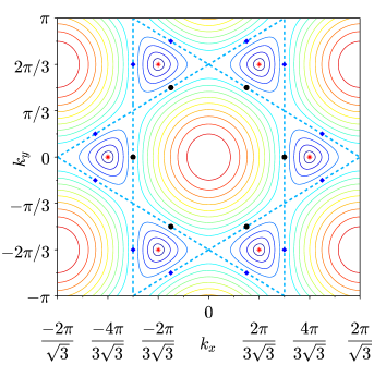
Figure 6: Level curves for the positive energy band of graphene without any SO couplings. ($k_{x},~{}k_{y}$ are in units of $1/a$). The figure shows an area equal to three Brillouin zones and six Dirac points (red stars). The blue dashed line is the locus of points with $E=\gamma$. The six black dots at $(k_{x},k_{y})=(\pm\pi/(\sqrt{3}a),0)$ and $(\pm\pi/(2\sqrt{3}a),\pm\pi/(2a))$ are the no-spreading points in the first Brillouin zone where the second derivatives of $E(k_{x},k_{y})$ vanish. The blue diamonds denote the corresponding points in the neighboring Brillouin zones and are related to the former set of points by reciprocal lattice vectors.

In Figs. 7(a) and 7(b), we show the time evolution of wave packets centered at two different points in momentum $(k_{x},k_{y})$, namely, the origin $(0,0)$ and a no-spreading point $(-\pi/(2\sqrt{3}a),-\pi/(2a))$; at $t=0$, the wave packets are taken to have real space width $W_{x}=W_{y}=8$ in units of the lattice spacing $a$. At $(k_{x},k_{y})=(0,0)$, the energy spectrum is flat; hence the group velocity $\vec{v}_{g}$ is zero along both $x$ and $y$ directions. Thus a wave packet with a peak momentum at $(0,0)$ which is centered around a point in real space continues to be centered around the same point as it evolves in time. However, it spreads uniformly in all directions as $\partial^{2}E/\partial k_{x}^{2}$ and $\partial^{2}E/\partial k_{x}^{2}$ are non-zero and equal, while $\partial^{2}E/\partial k_{x}\partial k_{y}=0$. The behavior of such a wave packet is shown in Fig. 7(a). We find that the wave packet spreads out isotropically; the spread increases linearly with time at long times (Fig. 8). In contrast to this, at $(k_{x},k_{y})=(-\pi/(2\sqrt{3}a),-\pi/(2a))$, the group velocity is non-zero but the second derivatives of $E$ are zero. As Fig. 7(b) shows, a wave packet centered around this momentum moves but does not spread.

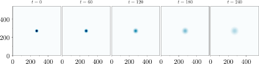
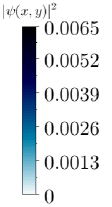
(a)  Wave packet with peak momentum ${\vec{k}}_{0}=(0,0).$

(b)  Wave packet with peak momentum ${\vec{k}}_{0}=(-\pi/(2\sqrt{3}a),-\pi/(2a)).$

Figure 7: Evolution of a Gaussian wave packet created in graphene without any SO couplings at $t=0$ with width $W_{x}=8a$ and $W_{y}=8a$. The $x$ and $y$ coordinates (horizontal and vertical directions respectively) are in units of $a$ while $t$ is in units of $\hbar/\gamma$. In (a), since the group velocity $\vec{v}_{g}(k_{x}=0,k_{y}=0)=\nabla_{{\vec{k}}}{E}|_{(0,0)}=(0,0)$, the wave packet does not move. But it spreads as $\partial^{2}E/\partial k_{x}^{2}$ and $\partial^{2}E/\partial k_{y}^{2}$ are non-zero. In (b), $\vec{v}_{g}(k_{x}=-\pi/(2\sqrt{3}a),k_{y}=-\pi/(2a))\neq 0$ but the second derivatives of $E$ vanish; this momentum is one of the no-spreading points shown in Fig. 6. Hence this wave packet moves but does not spread.

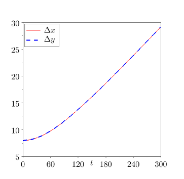
Figure 8: Spreads $\Delta x$ and $\Delta y$ in the $x$ and $y$ directions of the wave packet with peak momentum ${\vec{k}}_{0}=(0,0)$ as a function of time. (Both $\Delta x$ and $\Delta y$ are in units of $a$ while $t$ is in units of $\hbar/\gamma$). The time evolution of the wave packet is shown in Fig. 7(a).

IV.2 Periodic potential barriers

Next we look at the behavior of a wave packet when periodic potential barriers of the form shown in Fig. 1 are present. We first consider a wave packet whose momentum components are centered around one of the no-spreading points ${\vec{k}}_{0}=(-\pi/(2\sqrt{3}a),-\pi/(2a))$. Since each barrier is quite high ($C=\gamma$) and the wave packet has no components close to any of the Dirac points, there is almost no Klein tunneling and the reflection probability is close to 1. Hence the wave packet just reflects back and forth and stays between two successive barriers. This is shown in Fig. 9(a). The wave packet becomes narrower at the instant when it hits a barrier and is about to reflect back; this is visible in the second and fourth panels of Fig. 9(a). However, the width of the wave packet does not change when it is far from the barriers.

In contrast, when a wave packet is built with momenta centered around ${\vec{k}}_{0}=(4\pi/(3\sqrt{3}a),\pi/(5a))$ which lies close to a Dirac point, we see in Fig. 9(b) that it Klein tunnels through the barriers, each of height $C=(2/3)\gamma$. Since a narrower wave packet spreads faster, we have chosen a larger width $W_{x}=W_{y}=16a$ in order to clearly show the Klein tunneling near the Dirac point. Note that we have not taken the wave packet to be centered around a Dirac point exactly since the group velocity is not well defined at those points.

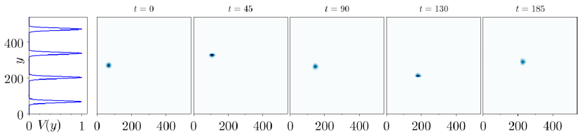
(a)  Wave packet with peak momentum ${\vec{k}}_{0}=(-\pi/(2\sqrt{3}a),-\pi/(2a))$.

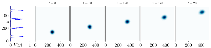
(b)  Wave packet with peak momentum ${\vec{k}}_{0}=(4\pi/(3\sqrt{3}a),\pi/(5a))$.

Figure 9: Evolution of a Gaussian wave packet in graphene without any SO couplings in the presence of equally spaced barriers of strength $C=\gamma$; the spacing between the barriers is $d=135a$, i.e., 90 unit cells. The $x$ and $y$ coordinates (horizontal and vertical directions respectively) are in units of $a$ while $t$ is in units of $\hbar/\gamma$. The leftmost panels show the positions of the barriers. In (a) the wave packet has width $W_{x}=W_{y}=8a$ at $t=0$. Due to the large barrier height, it almost completely reflects back and forth between two barriers. However it does not spread as it is centered around the no-spreading point $(-\pi/(2\sqrt{3}a),-\pi/(2a))$ in momentum space. In (b) the wave packet has initial width $W_{x}=W_{y}=16a$ and is centered around $(4\pi/(3\sqrt{3}a),\pi/(5a))$ which is close to a Dirac point. It almost completely Klein tunnels through the barriers, each of strength $C=(2/3)\gamma$.

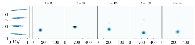
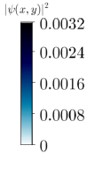
(a)  Gapped mode

(b)  Gapless mode

Figure 10: Evolution of a Gaussian wave packet in graphene with $\Delta_{KM}=\lambda_{R}=0.1\gamma$, and equally spaced barriers with strengths $C=\gamma$ and spacing $d=135a$. The $x$ and $y$ coordinates (horizontal and vertical directions respectively) are in units of $a$ while $t$ is in units of $\hbar/\gamma$. In momentum space the wave packet is centered around ${\vec{k}}_{0}=(4\pi/(3\sqrt{3}a),\pi/(5a))$, i.e., close to a Dirac point. Since $\Delta_{KM}=\lambda_{R}$, we have both gapless and gapped Dirac states. In (a) we see that the gapped mode almost completely reflects back and forth between two successive barriers (a small amount of transmission is faintly visible), whereas in (b) the gapless mode Klein tunnels through the barriers (a small amount of reflection is visible).

IV.3 Effect of spin-orbit couplings

We finally consider the case when both Kane-Mele and Rashba SO couplings are present and are of equal strength, i.e., $\Delta_{KM}=\lambda_{R}$. As discussed in Sec. II and shown in Fig. 2, the dispersion in this case has both gapped and gapless states close to the Dirac point. We look at these two kinds of states separately. In both cases we start with a wave packet with width $W_{x}=W_{y}=16a$ and peak momentum ${\vec{k}}_{0}=(4\pi/(3\sqrt{3}a),\pi/(5a))$. If the initial wave packet is constructed from the gapped states which have a non-relativistic dispersion, we find that there is almost complete reflection from the barriers. As shown in Fig. 10(a) the wave packet is trapped between two barriers, each of height $C=1$. The gapless mode however has a massless relativistic dispersion and just Klein tunnels through these barriers. Figure 10(b) depicts this case. We see that a small amount of reflection occurs when the wave packet crosses the barrier. This is because, as in Fig. 10(a), we have taken the peak momentum to be at ${\vec{k}}_{0}=(4\pi/(3\sqrt{3}a),\pi/(5a))$ which is slightly away from the Dirac point lying at $K=(4\pi/(3\sqrt{3}a),0)$; hence the Klein tunneling is not perfect. (Note that this wave packet is at normal incidence in the continuum language because the deviation of ${\vec{k}}_{0}$ from $K$ is zero in the $x$-direction).

V Discussion

In this paper we have studied the effects of SO couplings and a periodic potential on the dispersion and wave packet dynamics of electrons in graphene. We have considered both Kane-Mele and Rashba SO couplings and have shown that they have interesting effects, particularly when their magnitudes are equal.

We have first considered the continuum theory around the Dirac points to study the effects of a periodic potential. While a periodic potential is known to generate new Dirac points, we have shown that SO couplings generally open gaps at those points. However, when the Kane-Mele and Rashba SO couplings are equal in magnitude, some of the gapless Dirac points are restored. We have shown analytically that this occurs because equal Kane-Mele and Rashba SO couplings produce two kinds of states, with massless Dirac and massive Dirac forms respectively; at normal incidence, the massless states transmit perfectly through an arbitrary potential, and therefore no gaps are generated at the ends of the Brillouin zone when a periodic potential is present. Next, we have used a lattice model to study the effect of a single potential barrier. Using the momentum along the barrier as a good quantum number effectively reduces the system to a one-dimensional lattice. We have shown that the energy spectrum obtained using the lattice model reproduces those found with the continuum theory. In addition, we find some additional states which are localized along the barrier. These states have an interesting spin and sublattice structure arising from the SO couplings. Finally, we have used the lattice model to study the time evolution of a wave packet; the wave packet is taken to be a Gaussian. Without the SO couplings, we discover that there are six points in the momentum space such that a wave packet centered around these points shows almost no spreading; we call these the no-spreading points and we identify them by the condition that all the second derivatives of the energy with respect to the momenta should be zero. In the absence of SO couplings, we show that a wave packet centered around a Dirac point Klein tunnels through a barrier at normal incidence as expected. In the presence of equal Kane-Mele and Rashba SO couplings, we show that the massless Dirac states Klein tunnels at normal incidence while the massive Dirac states reflect when the barrier is high.

The no-spreading points lie at an energy of $\gamma\simeq 2.8$  eV which is quite far from the Dirac points (i.e., the Fermi energy of undoped graphene). It is therefore not easy to access them experimentally. One way of studying the dynamics at such points may be to inject an electron with that energy at one point of the system and then measure the probability of detecting it at another point. However, such an experiment may be difficult to perform because the large distance from the Fermi energy implies that the lifetime of the electron would be small. Even if it is difficult to study the no-spreading points in the immediate future, we have discussed them in this paper because they are so unusual. While no-spreading points are not uncommon in one-dimensional systems, graphene is the only example of a two-dimensional system that we know of which has such no-spreading points.

Our results can be tested experimentally by preparing samples of graphene with strong SO couplings. While the intrinsic SO coupling in graphene is very weak, one can induce SO couplings in a variety of ways weeks11 ; kou13 ; zhang14 ; zollner15 , and the strength of the induced SO couplings can be tuned experimentally. For instance, Ref. gmitra09, shows using a first principles calculation that the Kane-Mele and Rashba SO couplings can be made equal by applying a transverse electric field equal to $2.44$ V/nm. Finally, our work may also be applicable to other two-dimensional materials like silicene, germanene and stanene whose lattice structures are similar to graphene but with intrinsic spin-orbit couplings which are much stronger than in graphene liu11 ; rachel14 .

References

- (1)
- (2) C. W. J. Beenakker, Rev. Mod. Phys. 80, 1337 (2008).
- (3) A. H. Castro Neto, F. Guinea, N. M. R. Peres, K. S. Novoselov, and A. K. Geim, Rev. Mod. Phys. 81, 109 (2009).
- (4) S. Das Sarma, S. Adam, E. H. Hwang, and E. Rossi, Rev. Mod. Phys. 83, 407 (2011).
- (5) M. O. Goerbig, Rev. Mod. Phys. 83, 1193 (2011).
- (6) D. N. Basov, M. M. Fogler, A. Lanzara, F. Wang, and Y. Zhang, Rev. Mod. Phys. 86, 959 (2014).
- (7) K. S. Novoselov, A. K. Geim, S. V. Morozov, D. Jiang, M. I. Katsnelson, I. V. Grigorieva, S. V. Dubonos, and A. A. Firsov, Nature 438, 197 (2005).
- (8) Y. Zhang, Y.-W. Tan, H. L. Stormer, and P. Kim, Nature 438, 201 (2005).
- (9) M. I. Katsnelson, K. S. Novoselov, and A. K. Geim, Nature Phys. 2, 620 (2006).
- (10) V. Lukose, R. Shankar, and G. Baskaran, Phys. Rev. Lett. 98, 116802 (2007).
- (11) C. W. J. Beenakker, Phys. Rev. Lett. 97, 067007 (2006).
- (12) S. Bhattacharjee and K. Sengupta, Phys. Rev. Lett. 97, 217001 (2006).
- (13) S. Bhattacharjee, M. Maiti, and K. Sengupta, Phys. Rev. B 76, 184514 (2007).
- (14) M. Titov and C. W. J. Beenakker, Phys. Rev. B 74, 041401(R) (2006).
- (15) M. Maiti and K. Sengupta, Phys. Rev. B 76, 054513 (2007).
- (16) K. Sengupta and G. Baskaran, Phys. Rev. B 77, 045417 (2008).
- (17) M. Hentschel and F. Guinea, Phys. Rev. B 76, 115407 (2007).
- (18) T. O. Wehling, A. V. Balatsky, M. I. Katsnelson, A. I. Lichtenstein, and A. Rosch, Phys. Rev. B 81, 115427 (2010).
- (19) J.-H. Chen, L. Li, W. G. Cullen, E. D. Williams, and M. S. Fuhrer, Nature Phys. 7, 535 (2011).
- (20) B. Uchoa, T. G. Rappoport, and A. H. Castro Neto, Phys. Rev. Lett. 106, 016801 (2011).
- (21) V. V. Cheianov and V. I. Fal’ko, Phys. Rev. Lett. 97, 226801 (2006).
- (22) E. Mariani, L. I. Glazman, A. Kamenev, and F. von Oppen, Phys. Rev. B 76, 165402 (2007).
- (23) C. Bena, Phys. Rev. Lett. 100, 076601 (2008).
- (24) C. Bena, Phys. Rev. B 79, 125427 (2009).
- (25) A. V. Shytov, M. I. Katsnelson, and L. S. Levitov, Phys. Rev. Lett. 99, 246802 (2007).
- (26) Y. Wang, D. Wong, A. V. Shytov, V. W. Brar, S. Choi, Q. Wu, H. Z. Tsai, W. Regan, A. Zettl, R. K. Kawakami, S. G. Louie, L. S. Levitov, M. F. Crommie, Science 340, 734 (2013).
- (27) C. L. Kane and E. J. Mele, Phys. Rev. Lett. 95, 146802 (2005).
- (28) C. L. Kane and E. J. Mele, Phys. Rev. Lett. 95, 226801 (2005).
- (29) E. I. Rashba, Phys. Rev. B 79, 161409(R) (2009).
- (30) M. Zarea and N. Sandler, Phys. Rev. B 79, 165442 (2009).
- (31) C. Dutreix, M. Guigou, D. Chevallier, and C. Bena, Eur. Phys. J. B 87, 296 (2014).
- (32) R. Seshadri, K. Sengupta, and D. Sen, Phys. Rev. B 93, 035431 (2016).
- (33) M.-H. Liu, J. Bundesmann, and K. Richter, Phys. Rev. B 85, 085406 (2012).
- (34) M. Gmitra, S. Konschuh, C. Ertler, C. Ambrosch-Draxl, and J. Fabian, Phys. Rev. B 80, 235431 (2009).
- (35) C. Weeks, J. Hu, J. Alicea, M. Franz, and R. Wu, Phys. Rev. X 1, 021001 (2011).
- (36) L. Kou, B. Yan, F. Hu, S.-C. Wu, T. O. Wehling, C. Felser, C. Chen, and T. Frauenheim, Nano Letters 13, 6251 (2013).
- (37) J. Zhang, C. Triola, and E. Rossi, Phys. Rev. Lett. 112, 096802 (2014).
- (38) K. Zollner, T. Frank, S. Irmer, M. Gmitra, D. Kochan, and J. Fabian, Phys. Rev. B 93, 045423 (2016).
- (39) D. R. da Costa, A. Chaves, G. A. Farias, L. Covaci, and F. M. Peeters, Phys. Rev. B 86, 115434 (2012).
- (40) G. M. Maksimova, V. Ya. Demikhovskii, and E. V. Frolova, Phys. Rev. B 78, 235321 (2008).
- (41) A. Singh, T. Biswas, T. K. Ghosh, and A. Agarwal, Eur. Phys. J. B 87, 275 (2014).
- (42) A. Singh, T. Biswas, T. K. Ghosh, and A. Agarwal, Annals of Physics 354, 274 (2015).
- (43) C.-H. Park, L. Yang, Y.-W. Son, M. L. Cohen, and S. G. Louie Phys. Rev. Lett. 101, 126804 (2008).
- (44) L. Brey and H. A. Fertig, Phys. Rev. Lett. 103, 046809 (2009).
- (45) M. Barbier, P. Vasilopoulos, and F. M. Peeters, Phys. Rev. B 81, 075438 (2010).
- (46) M. Barbier, P. Vasilopoulos, and F. M. Peeters, Phil. Trans. R. Soc. A 368, 5499 (2010).
- (47) S. Dubey, V. Singh, A. K. Bhat, P. Parikh, S. Grover, R. Sensarma, V. Tripathi, K. Sengupta, and M. M. Deshmukh, Nano Lett. 13, 3990 (2013).
- (48) M. Drienovsky, F.-X. Schrettenbrunner, A. Sandner, D. Weiss, J. Eroms, M.-H. Liu, F. Tkatschenko, and K. Richter, Phys. Rev. B 89, 115421 (2014).
- (49) S.-K. Choi, C.-H. Park, and S. G. Louie, Phys. Rev. Lett. 113, 026802 (2014).
- (50) Kh. Shakouri, M. R. Masir, A. Jellal, E. B. Choubabi, and F. M. Peeters, Phys. Rev. B 88, 115408 (2013).
- (51) R. Seshadri and D. Sen, Phys. Rev. B 89, 235415 (2014).
- (52) D. Sen and O. Deb, Phys. Rev. B 85, 245402 (2012); Erratum, Phys. Rev. B 86, 039902(E) (2012).
- (53) C.-C. Liu, H. Jiang, and Y. Yao, Phys. Rev. B 84, 195430 (2011).
- (54) S. Rachel and M. Ezawa, Phys. Rev. B 89, 195303 (2014).