De-noising the galaxies in the Hubble XDF with EMPCA

Abstract

We present a method to model optical images of galaxies using Expectation Maximization Principal Components Analysis (EMPCA). The method relies on the data alone and does not assume any pre-established model or fitting formula. It preserves the statistical properties of the sample, minimizing possible biases.

The precision of the reconstructions appears to be suited for photometric, morphological and weak lensing analysis, as well as the realization of mock astronomical images. Here, we put some emphasis on the latter because weak gravitational lensing is entering a new phase in which systematics are becoming the major source of uncertainty. Accurate simulations are necessary to perform a reliable calibration of the ellipticity measurements on which the final bias depends.

As a test case, we process $7038$ galaxies observed with the ACS/WFC stacked images of the Hubble eXtreme Deep Field (XDF) and measure the accuracy of the reconstructions in terms of their moments of brightness, which turn out to be comparable to what can be achieved with well-established weak-lensing algorithms.

1 Introduction

Optical imaging is without any doubt one of the main tools to investigate galaxies and dark matter through weak and strong gravitational lensing. Because of the large available data sets, it is crucial to extract all information available in noisy data and to simulate images precisely to calibrate the various methods and properly deal with possible biases. There is thus a pressing need to extract clean galaxy images from data.

In particular, several studies have shown how all methods used to measure the ellipticity of galaxies require realistic simulations for their calibration (Viola et al., 2011; Bartelmann et al., 2012; Refregier et al., 2012; Melchior & Viola, 2012; Massey et al., 2013; Gurvich & Mandelbaum, 2016; Bruderer et al., 2016). This issue is becoming pressing because of the stringent requirements posed by upcoming wide-field surveys such as the ESA Euclid space mission (Laureijs, 2009) and the Large Synoptic Survey Telescope (Kaiser et al., 2002), among others. Galaxy models based on simple analytical recipes, for example based on the Sersic profile Sersic (1968), have been widely used at this end (Heymans et al., 2006; Bridle et al., 2010; Kitching et al., 2012). These models have proven to well suffice for ground-based observations, but more accurate simulations are now necessary to include complex morphologies to account for spiral, irregular and cuspy galaxies. Also in the strong gravitational lensing regime, accurate galaxy models are now needed to investigate the use of substructures of strongly magnified galaxies to better constrain the mass distribution of lenses such as for example galaxy clusters (Meneghetti et al., 2008; Zitrin et al., 2015).

For these reasons, galaxies observed with HST have been modelled with shapelets (Refregier, 2003; Refregier & Bacon, 2003; Massey et al., 2004; Massey et al., 2007) to achieve noise-free images. Even if this approach deals with complex morphologies, artifacts may arise because of the oscillatory behavior of shapelets. Moreover, also smooth galaxies such as for example ellipticals are not very well reconstructed by this approach because of their slope, which is not well compatible with a Gaussian, which the Hermite polynomials in the shapelets are derived from. Also, image cut-outs have been extracted from HST data (Rowe et al., 2015; Mandelbaum et al., 2015), but these stamps are affected by the instrumental noise limiting their applicability.

In this paper, we present a method to retrieve and reconstruct clean galaxy images in a model-independent way, which also preserves the statistical properties of the reconstructed sample. We do this using Expectation Maximization Principal Components Analysis Bailey (2012), which we use to derive a set of orthonormal basis functions optimized for the specific data set to be processed. Other studies used standard PCA (Jolliffe, 2002) to model elliptical galaxies (Joseph et al., 2014). However, these are galaxies with smooth morphology, and this method cannot deal with weights and missing data. In contrast, the procedure discussed in this work allows us to process astronomical images with masked areas and pixel-dependent variance, and it allows us to introduce regularization terms to be used when deriving the principal components and impose smoothness on the basis.

Figure 1: This schematic representation shows how a postage-stamp of a galaxy image is rearranged in form of a vector, $\mn@boldsymbol{d}_{i}$. All rows of pixels in the matrix composing the image are simply concatenated.

Figure 2: Statistical properties of the sources detected in the simulation and reproducing a Subaru image with 20 minutes of exposure time. A comparison with the real data is provided. From left to right, the panels show the magnitude distribution of the objects, their photometric error as a function of magnitude, and their size versus magnitude relation.

As a test case, we analyzed $7038$ galaxies extracted from the Rafelski et al. (2015) catalog with redshift up to $z<4.0$ and maximum magnitude up to $m_{F775W}<30$. The catalog contains all photometric information including the photometric redshifts of the objects. We modeled these galaxies in all 5 optical bands extracted from the Hubble eXtreme Deep Field (XDF hereafter, Illingworth et al., 2013). We tested the quality of the models by comparing their moment of brightness against those measured with the weak-lensing Shapelens library (Melchior et al., 2011). Moreover we showed how to use these models to construct realistic simulations of astronomical images.

The structure of this paper is a follows: in Sec. (2), we derive the EMPCA which are then used in Sec. (5) to create the models of the galaxy images. The description of the analysis of the XDF data set in Sec. (5), a simple sky simulation based on our models is presented in Sec. (6), and the conclusions are given in Sec. (7).

2 A linear model for galaxy images

In this section, we discuss how to model the images of individual galaxies to obtain a noise-free reconstruction. Let us now consider the case in which we have one single object placed in the center of a postage-stamp. This cut-out can be modeled as

$$d(\mn@boldsymbol{x})=g(\mn@boldsymbol{x})+n(\mn@boldsymbol{x})\;,$$ (1)

where $g(\mn@boldsymbol{x})$ is the object contribution we are interested in, $n(\mn@boldsymbol{x})$ the one of the noise (e.g. photon noise, read-out noise, dark current), and $\mn@boldsymbol{x}\in\mathbb{R}^{2}$ denotes the position in the image. For simplicity, we assume the noise to be uncorrelated with standard deviation $\sigma$, defined by $\langle n_{i}\,n_{j}\rangle=\sigma^{2}\,\delta(i-j)$. This 2-dimensional image $d(\mn@boldsymbol{x})$, consisting of $n=n_{x}\times n_{y}$ pixels, can be represented as a data vector $\mn@boldsymbol{d}\in\mathbb{R}^{n}$ whose elements $d(x_{i})=d_{i}$ are the intensities of the $i_{th}$ pixels. A visual impression of how pixels are rearranged in a vector is shown in Figure (1).

The most general linear model to describe this data element is

$$\tilde{d}(\mn@boldsymbol{x})=\sum_{k=1}^{M}a_{k}\phi_{k}(\mn@boldsymbol{x})\;,$$ (2)

where $\mn@boldsymbol{\phi}_{k}\;$ is a collection of $M$ vectors, $\left\{\mn@boldsymbol{\phi}_{k}\;\in\;\mathbb{R}^{n}\;\mid\;k=1,...,M\right\}$. The goal now is to define an optimal set of vectors $\phi_{k}$ capturing the relevant signal and sort them depending on their information content (power) such that each vector contains more information than the following one.

Once this is achieved, the sm can be split into two terms

$$d(\mn@boldsymbol{x})=\sum_{k=1}^{M}a_{k}\phi_{k}(\mn@boldsymbol{x})+\sum_{M+1}^{n}a_{k}\phi_{k}(\mn@boldsymbol{x})=\tilde{g}(\mn@boldsymbol{x})+\tilde{n}(\mn@boldsymbol{x})\;,$$ (3)

where now $\tilde{g}(\mn@boldsymbol{x})$ is the model of the object we are interested in, and $\tilde{n}(\mn@boldsymbol{x})$ a term containing most of the noise and a small, and hopefully negligible, amount of information. The number of components, $M$, fixes the amount of information which is going to be kept in the model and the amount of noise which is going to be suppressed. Some information loss is inevitable, otherwise one could fully recover the real image of the object which is obviously an impossible task. A common way to achieve this decomposition is provided by the Principal Component Analysis (PCA hereafter, Jolliffe, 2002) which takes advantage of the entire data set, i.e. the postage-stamps of all galaxies in the sample, $\left\{\mn@boldsymbol{d}_{j}\;\in\;\mathbb{R}^{n}\;\mid\;j=1,...,s\right\}$, and consists in finding the set of vectors, $\mn@boldsymbol{\phi}_{k}\;\in\;\mathbb{R}^{n}$, minimizing the quantity

$$\chi^{2}=\sum_{ij}^{n,s}\left(d_{ij}-\sum^{n}_{k=1}a_{kj}\phi_{ki}\right)^{2}\;.$$ (4)

In other words, we are looking for the model based on all coefficients, $a_{jk}$, and vectors, $\mn@boldsymbol{\phi}_{k}$, which best fit all images at once. Here and throughout the paper, the index $i$ runs over the number of pixels, $j$ over the number of galaxies, and $k$ over the number of components which, in the case of the PCA, is equal to the number of pixels. The coefficients of the $j_{th}$ galaxy are derived with the scalar product $a_{kj}=\sum_{i}d_{ji}\phi_{ki}$ or by linear fitting if needed. Equation (4) can be easily generalized to account for correlated noise.

Figure 3: First six principal components, $\mn@boldsymbol{\phi}_{i}$, derived from the noisy simulated image. The components are rearranged as images. From the data emerge the main features related to dipolar and quadrupolar structures as well as radially symmetric ones.

Figure 4: One of the galaxies randomly extracted from the simulation for which we show the signal and noise splitting: in the left panel the original postage-stamps, $\mn@boldsymbol{d}_{j}$, the model, $\mn@boldsymbol{\tilde{g}_{j}}$ in the center and the residuals, $\mn@boldsymbol{\tilde{n}_{j}}$ on the right.

Usually, the principal components are found by diagonalizing the centered covariance matrix of the data and ordering its eigenvectors by decreasing eigenvalues, $\lambda_{k}$. Another way to find the solution for the minimum of Equation (4) is through the Expectation Maximization Principal Components Analysis (EMPCA hereafter). This is an iterative algorithm which consists in finding one basis component at a time. To find the first component $\mn@boldsymbol{\phi}_{1}$, we start with a random vector (all its $n$ components have a random value) with which we compute the first coefficient of all objects through the scalar product previously defined, $a_{1j}=\sum_{i}d_{ji}\phi_{1i}$. These coefficients are then used to update $\mn@boldsymbol{\phi}_{1}$,

$$\phi_{1}^{new}(\mn@boldsymbol{x})=\frac{\sum_{j}^{s}a_{1j}d_{j}(\mn@boldsymbol{x})}{\sum_{j}^{s}a_{1j}^{2}}\;,$$ (5)

which is renormalized for convenience and which now will fit the data set better. The refined $\mn@boldsymbol{\phi}_{1}^{new}$ vector is subsequently used to compute a new set of $a_{1j}$ coefficients necessary for the next iteration, and so on. This procedure is converging toward the only absolute minimum of the $\chi^{2}$ function, as demonstrated by Srebro & Jaakkola (2003). In our case, this iterative process is stopped when the variation in the principal component, $\mn@boldsymbol{\phi}_{1}$, is smaller that a certain value, $|\Delta\phi_{1}|<\epsilon$, which we set to $\epsilon=10^{-6}$. The next principal component, $\mn@boldsymbol{\phi}_{k+1}$, is found by applying the same procedure to that part of the signal which has not been captured by the previous $k$ components,

$$\phi_{k+1}^{new}(\mn@boldsymbol{x})=\frac{\sum_{j}^{s}a_{k+1j}\,\tilde{n}_{j}(\mn@boldsymbol{x})}{\sum_{j}^{s}a_{k+1j}^{2}}\;.$$ (6)

Here, $\tilde{n}_{j}(\mn@boldsymbol{x})=d_{j}(\mn@boldsymbol{x})-\tilde{g}_{j}(\mn@boldsymbol{x})$ is the residual part of the signal for which this component is evaluated, and $\tilde{g}_{j}(\mn@boldsymbol{x})=\sum_{l=1}^{k}a_{lj}\phi_{l}(\mn@boldsymbol{x})$ is the updated model of the $j-th$ galaxy. In analogy to the derivation of the first component, the coefficients of the $j-th$ galaxy, $a_{k+1\,j}=\sum_{i}d_{ji}\phi_{k+1\,i}$, are based on the previous iteration, and $\mn@boldsymbol{\phi}_{k+1}^{new}$ is renormalized each time. With this procedure we compute at the same time the principal components, $\mn@boldsymbol{\phi}_{k}$, the noise, $\tilde{\mn@boldsymbol{n}}_{j}$, and the signal estimate, $\tilde{\mn@boldsymbol{g}}_{j}$, we are aiming at (see Equation 3). The procedure ensures the orthogonality of the principal components. The further advantages of this method with respect to a geometrical interpretation of the principal components are that it allows to take advantage of weights, masks and the noise covariance by including them in the $\chi^{2}$ function, and to impose further conditions on the basis such as for example a regularization term to obtain smooth basis components (Bailey, 2012).

Figure 5: Power of the principal components resulting for the simulation with Sersic galaxies (continuous line) and for the real Subaru image mimicked by the simulation (dashed line). The power has been normalized with respect to the total variance, $\sigma^{2}=\sum_{k}^{n}\lambda_{k}$. In both cases, their amplitude drops rapidly with the order.

Here, we have derived smooth principal components by bilateral smoothing during their construction. This is an edge-preserving algorithm with an adaptive smoothing scale which allows to leave those regions of the basis unaffected which show steep gradients that would be blurred otherwise. The bilateral smoothing implemented is based on the product of two Gaussians, one acting on angular scales as it would do a normal convolution and another based on the local luminosity gradient such that areas with “sharp” features do not get smoothed (if the gradient is small the angular convolution takes the lead, while it is made ineffective otherwise).

Alternatively, we used a different regularization scheme base on a Savitzky–Golay filter and obtained similar results. It is important to introduce this regularization during the basis construction and not thereafter (by smoothing the final basis or the models) to preserve the orthonormality of the basis, the information present in the data, and to make the basis more stable against noise fluctuations.

Additionally, we reduced the scatter in the galaxy morphologies by rotating the input images by multiples of $\pi/2$ such as to have their position angle range between 0 and $90$ degrees. We chose such discrete rotations instead of aligning the galaxies along their major axes to avoid the introduction of any pixel correlations.

Figure 6: Magnitude (left panel) and redshift distributions (right panel) of the sources with a maximum $\chi^{2}_{mod}$ of 4 for the BPZ redshift. The right panel shows the number of galaxies in the bins split according to their F775W magnitude.

In the following, we focus on the caveats of this approach which one should keep in mind to properly use it. First of all, the basis is derived from noisy data, and this will of course impact on them. This is relevant at higher orders where the EMPCA have to deal with smaller and less prominent features approaching the noise regime, as is clear from the discussion of Eq. (3). Second, the number of galaxies to produce the basis is limited, and a small sample will not be representative of the entire population. On the other hand, wide field surveys provide us with large data sets which even allow to split the sample into subsets of galaxies with similar properties (such as for example size or ellipticity) and further reduce the data scatter for a better optimization of the basis.

It is also preferable to compute the basis for the sample which has to be processed and not on another independent set of images even if with compatible size and quality. After all, the basis components are evaluated by finding the optimal model of the specific data at hand. Third, the regularization used to impose smoothness on the basis might decrease the level of high frequency features present in the data, if one wants to use it at all. In any case, one can always decide and adapt the regularization which better suits the case at hands.

One final remark about the point spread function (PSF): The PSF is not an issue for this approach because it aims at the image as it is. However, some care has to be taken if the models are going to be used for weak-lensing purposes because the PSF ellipticity and distortions may leave an imprint on the derived basis and thus on the models based on them. It is easy to cope with this issue with the procedure adopted in this work. In fact, the rotation applied to the postage-stamps prevents any isotropy which my be induced by the PSF.

3 Defining the number of components

As discussed in Section (2), the number of basis components, $M$, defines the amount of noise which is going to be suppressed and the amount of information which is going to be kept in the model. Its value depends on the specific task we have at hands. Various schemes for the definition of $M$ have been proposed in the literature, for instance through the analysis of the scree graph (Cattell, 1966; Cattell & Vogelmann, 1977) or the log-eigenvalue diagram (LEV) (S.A., 1971; Maryon, 1979; Beltrando, 1990). These approaches are not very stable because they largely depend on specific features of these diagrams which may not be well defined in certain cases. Other approaches rely on a $\chi^{2}$ approach,

$$\chi_{j}^{2}=\sum_{i=1}^{n}(d_{ij}-\tilde{g}_{ij})^{2}\,$$ (7)

applied to each individual galaxy (not the overall set!) and which better suits our needs (Ferré, 1990). Below, we discuss two criteria aiming at different goals.

1. Defining $M$ to minimize the model variance: if we search for the model $\tilde{g}$ with the minimum variance, it is necessary to minimize the number of basis components. Here we seek for the smallest $M$, which will be specific for each individual object, by including one component at a time until a certain convergence criteria is reached, for instance until we obtain a reduced $\chi^{2}$ close to unity or until the $\chi^{2}$ is not changing by more than a certain threshold. Formally this criterion reads $\left\{\,\mbox{min}\{k\}\in\mathbb{N}:\chi^{2}_{k}-\chi^{2}_{k+1}\leq t\,\right\}$, where $t$ is the threshold to be set. A note of caution is in order here: by construction, the $\chi^{2}$ is monotonically decreasing with the order (at the order $n$ the $\chi^{2}$ will be zero) and under- or over-fitting might be an issue. Moreover, the basis components are sorted by their information content (the higher the order, the less relevant is the component), but this sorting is based on the statistics of all objects in the sample and may not be proper for a specific object. It may happen that for a specific object, one of the higher-order components is more relevant than lower-order components, and the convergence process may stop before this component is reached.

2. Defining $M$ to maximize model fidelity: for ensuring not to miss any valuable signal, it is necessary to include all components, for instance by visually inspecting the basis or by finding the $M$ for which the expectation value of the global $\chi^{2}$ is the minimum. This $M$ can not be evaluated directly but it can be approximated by

   $$\hat{f}_{q}=\sum_{k=q+1}^{n}\hat{\lambda}_{k}+\sigma^{2}\left[2nq-n^{2}+2(n-q)+4\sum_{l=1}^{q}\sum_{k=q+1}^{n}\frac{\hat{\lambda}_{l}}{\hat{\lambda}_{l}-\hat{\lambda}_{k}}\right]\;,$$ (8)

   under the assumption of uncorrelated noise. Here, $\lambda_{k}$ is the power related to the $k-th$ component. The variance can be estimated as $\sigma^{2}_{q}=1/(n-q)\sum_{k=q+1}^{n}\lambda_{k}$ and $\hat{\lambda}_{k}=\frac{n-1}{n}\lambda_{k}$ (Ferré, 1990). With these criteria, $M$ is the same for all objects because it is based on the statistics of the entire data sample, in contrast to what we discussed in point (i) where the $\chi^{2}$ was evaluated for each individual object. This approach returns the highest “fidelity” because the largest number of sensible components is used.

4 Simulation of ground base observations

To test the quality of the model reconstruction, we produced a set of simulations with EasySky. EasySky allows to use any object contained in a postage-stamp image, Sersic galaxies, galaxies with a single or double Sersic components (bulge plus disc) in the same fashion as the Great08 (Bridle et al., 2010; Kitching et al., 2012) simulations, and stars with a Moffat profile and arbitrary ellipticity (if stars are to be included). The objects can be displaced in various ways: randomly across the whole field-of-view, on a regular grid with stars on one side and galaxies on the other, or on a regular grid but with the stars located equidistantly from the other galaxies. The galaxies can be (1) randomly rotated, (2) kept with their semi-major axes aligned with one direction, (3) within the same quadrant, or (4) produced in pairs with angles rotated by 90 degrees with respect to each other. The latter configuration is a useful feature for weak-lensing calibrations. The fluxes and sizes of both galaxies and stars can be kept fixed or randomly distributed following a given luminosity function to better re-sample the data to be simulated. The image can be convolved with an arbitrary kernel, and a simple shear distortion can be applied to the galaxies.

Figure 7: The first four principal components for three different sets of galaxies. The upper, middle and bottom rows refer to galaxies with semi-major axis, $A$, within the range $5<A<7$, $18<A<20$, $50<A<60$, and $70<A<80$ pixels, respectively. The larger the galaxies are, the larger is the typical size of the principal component and the larger is their morphological complexity.

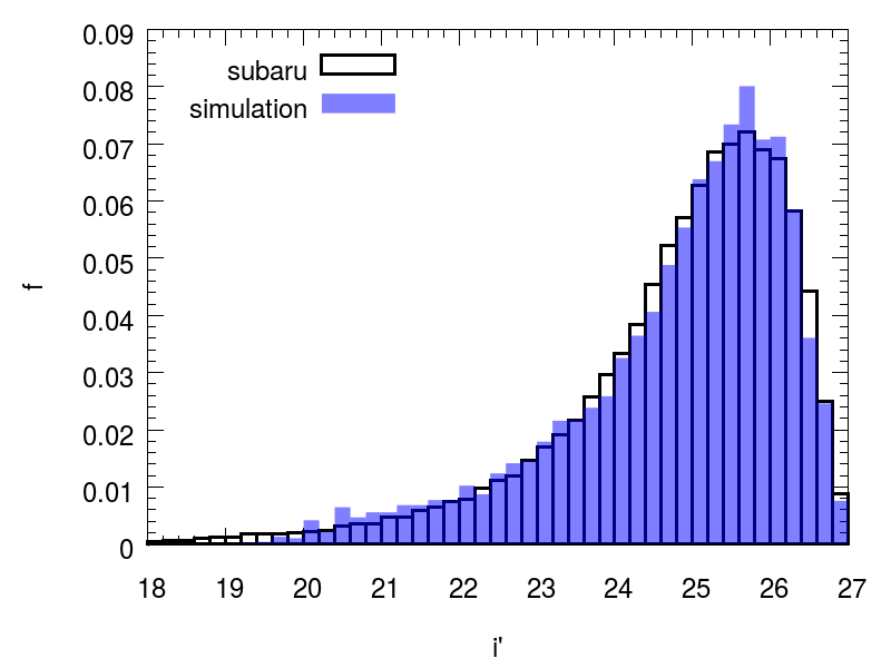
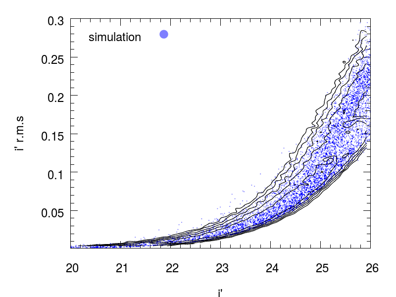
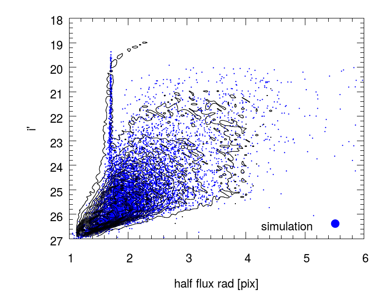
Here, we describe a simple but quite realistic synthetic image which we used to show the signal-to-noise splitting of Eq. (3). We included $10\,000$ galaxies located on a $100\times 100$ regular grid but with the centroid displaced by a random shift within $1.5$ pixels. The galaxies are characterized by a Sersic profile (Sersic, 1968) with a fixed index $n=2$. They are convolved with a PSF described by a Moffat function with $\beta=4.8$, $\mbox{FWHM}=4.45$ pixels (Moffat, 1969), and a complex ellipticity $g_{PSF}=-0.019-i\,0.007$, adapted to the fiducial values adopted in Great08 (Bridle et al., 2010). The noise variance, the source fluxes, scale radii and ellipticities have been randomly distributed such as to resemble those of a stacked image obtained with the OmegaCam mounted on the Subaru telescope and 20 minutes of total exposure time in the $i^{\prime}$ filter. A comparison of the magnitude distribution, the photometric errors and the size-magnitude relation between the simulated images and a real Subaru image is shown in Fig. (2).

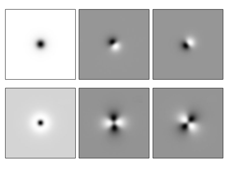
The simulation has been processed as it would be with a real image, i.e. detecting the sources, separating galaxies from stars with SExtractor (Bertin & Arnouts, 1996), and creating postage-stamps sized $60\times 60$ pixels for each object based on the measured astrometry. In this case, we did not apply any rotation to the galaxy images for simplicity. This will be done in the more sophisticated simulation discussed in Sec. (6) below. The principal components, $\mn@boldsymbol{\phi}_{i}$, obtained for this sample are shown in Fig. (3), where for visualization purposes only we inverted the process sketched in Fig. (1) to rearrange the vectors in form of an image.

It is interesting to note how the data deliver principal components with radially symmetric profiles ($w_{1}$ and $w_{4}$), dipolar ($w_{2}$ and $w_{3}$), and quadrupolar ($w_{5}$ and $w_{6}$) structures as well. Higher modes show hexapoles and more complex structures. It is easy to interpret these shapes: for instance the circularly symmetric components take care for the average brightness profile, while the dipolar ones account for a large fraction of the object’s ellipticity.

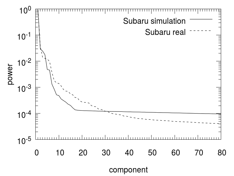
In Fig. (5), we show the power of the principal components normalized by the total variance, $\sigma^{2}=\sum_{k}^{n}\lambda_{k}$. The continuous line represents the simulation, and the dashed line the real SUBARU image mocked by the simulation. In both cases, the power of the components drops rapidly with their order, and the same kinks are visible in the curves. The drop in power is less dramatic for real data because of the more complex morphology of the galaxies. At orders higher than $15$, there is a clear plateau for the simulated images because here we enter the regime of uncorrelated random noise containing no more features. The real image lacks such a plateau because in this case the noise is correlated because the image results from stacking.

Figure 8: Four galaxies extracted from the XDF sample. From left to right, the columns show: the original image (with other objects present in the postage-stamp already removed), the model generated with the EMPCA, the model residuals, and the segmentation of the image we derived from the model. The image of the smaller galaxies has been enlarged for visualization purposes.

An example for the signal-to-noise splitting, $d(\mn@boldsymbol{x})=\tilde{g}(\mn@boldsymbol{x})+\tilde{n}(\mn@boldsymbol{x})$, discussed in Sec. (2), is displayed in Fig. (4) where, from left to right, we show the original data $\tilde{d}(\mn@boldsymbol{x})$, the model $\tilde{g}(\mn@boldsymbol{x})$, and the residuals $\tilde{n}(\mn@boldsymbol{x})$. The maximum order $M$ has been determined with the criterion $\left\{\,\mbox{min}\{k\}\in\mathbb{N}:\chi^{2}_{k}-\chi^{2}_{k+1}\leq t\,\right\}$, setting $t=0.005$. As expected, the galaxy model is compact, i.e. it vanishes at a certain distance form the center of the galaxy, most of the noise is removed from the image, and the residuals are fully uncorrelated.

A more quantitative assessment of the reconstruction quality, based on the brightness moments of the images, is discussed in Sect. (6) where we deal with galaxies with complex morphologies.

5 Modeling the XDF galaxies

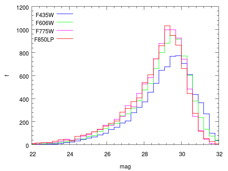
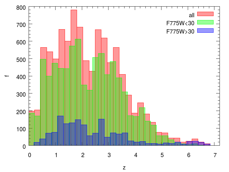
We now come to the full analysis of real data. Here, we processed the ACS/WFC stacked images of the Hubble eXtreme Deep Field (XDF, hereafter, see Illingworth et al., 2013) which covers an area of $10.8$ arcmin² down to the $\sim 30$ AB magnitude ($5\sigma$). The images are drizzled with a scale of $0^{\prime\prime}.03$ pixel^-1 and have been obtained with the F435W, F606W, F775W, F814W, and F850LP filters for a total exposure time of $1177$ks. We used all objects listed in the UVUDF catalog which are classified as galaxies (Rafelski et al., 2015). To avoid artifacts and truncated objects, we discarded those objects in the areas affected by the ghosts and halos of stars or close to the edges of the survey. In this way, we selected 8543 galaxies from an effective area of $9.20$ arcmin². We further cut the sample by rejecting all galaxies with an F775W magnitude larger than $30$, ending up with 7038 objects. The redshift and magnitude distributions of the sources with a maximum $\chi^{2}_{mod}$ of 4 for the BPZ redshift are shown in Fig. (6).

Figure 9: A collection of galaxy models obtained with the EMPCA and based on the F435W, F606W, and F775W filters. The first and second top panels show the same objects displayed in Fig. (8). The size of each box is of $5.4$ arcsec.

Figure 10: Four simulations realized with EasySky displaying a field of $0.65\times 0.65$ arcmin² observed with the F775W filter without noise (upper left panel), with a XDF like noise (upper right panel), a noise equivalent to one HST orbit (bottom left), and a CFHTLens-quality image for a seeing of $0.7$ arcsec (bottom right panel).

When computing the principal components, we split the sample in groups of galaxies with similar size, and evaluate the basis for each of these subsamples separately. This is to obtain a collection of basis sets, one per sub-sample, which is optimized for galaxies with that specific size. If we used all galaxies at once, the features captured by the EMPCAs will be distributed on a larger number of components because then the range of sizes they have to reproduce will be larger.

To further reduce the amount of scatter in the data, we rotated the galaxies by $90$ deg, whenever necessary, to align them within the same quadrant. We did not align the galaxies’ major axes along the same direction to avoid the introduction of additional correlation among the pixels for a marginal improvement that could barely be justified.

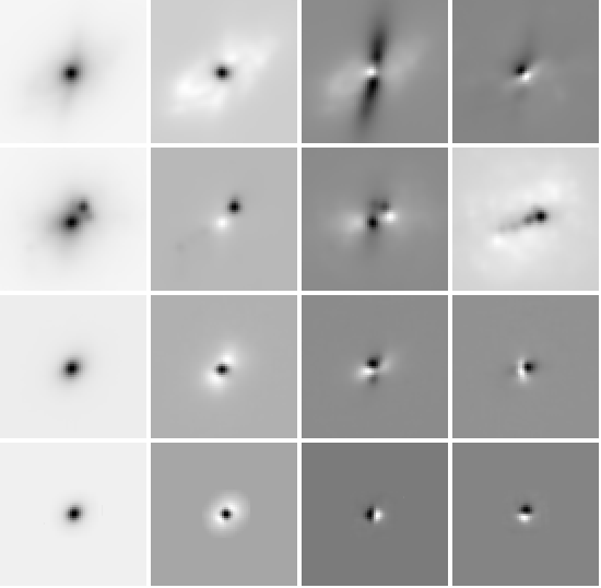
We finally take advantage of all bands by including all of them in the training sets. This further reduces the noise and enriches the number of features which can be reproduce with the same basis set. In Fig. (7), we plot the first four principal components computed for three different sub-sets of galaxies with semi-major axis, $A$, within the ranges $5<A<7$, $18<A<20$, $50<A<60$, and $70<A<80$ pixels for the first, second, third and forth rows, respectively. The semi-major axes, $A=\sqrt{I(1-e)/\pi}$, was derived from the isophotal area, $I$, and the object ellipticity, $e$, which turned out to be a suitable choice for our pourpose. As expected, the larger the galaxies in the training sample are, the larger is the typical scale of the EMPCA. Additionally, one can see that larger galaxies show principal components with more complex features because of their larger variety in morphology and substructure.

Having computed the basis for each sub-sample, we use them to create the galaxy models as discussed in Sec. (2). Since some of the variance due to the noise is still present in the model, which is unavoidable in general, we set all pixels to zero with amplitude less than $t=\sigma/5$, where $\sigma$ is the pixel variance of the original image. This is to avoid such areas of the image which, in fact, do not show any evidence of signal. The code to perform the overall analysis is called EasyEMPCA.

Figure 11: Dispersion around the true value of the brightness moments of the models reconstructed with EMPCA (blue) and as measured with Shapelens (red).

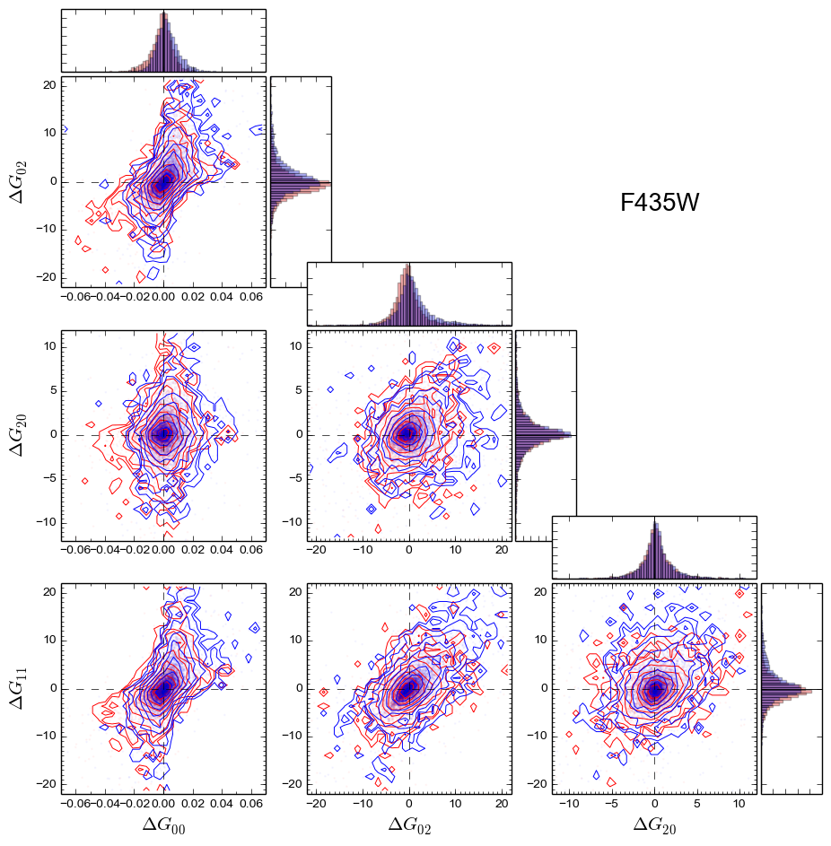
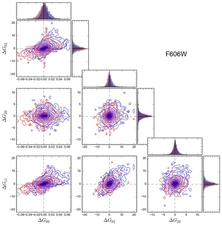
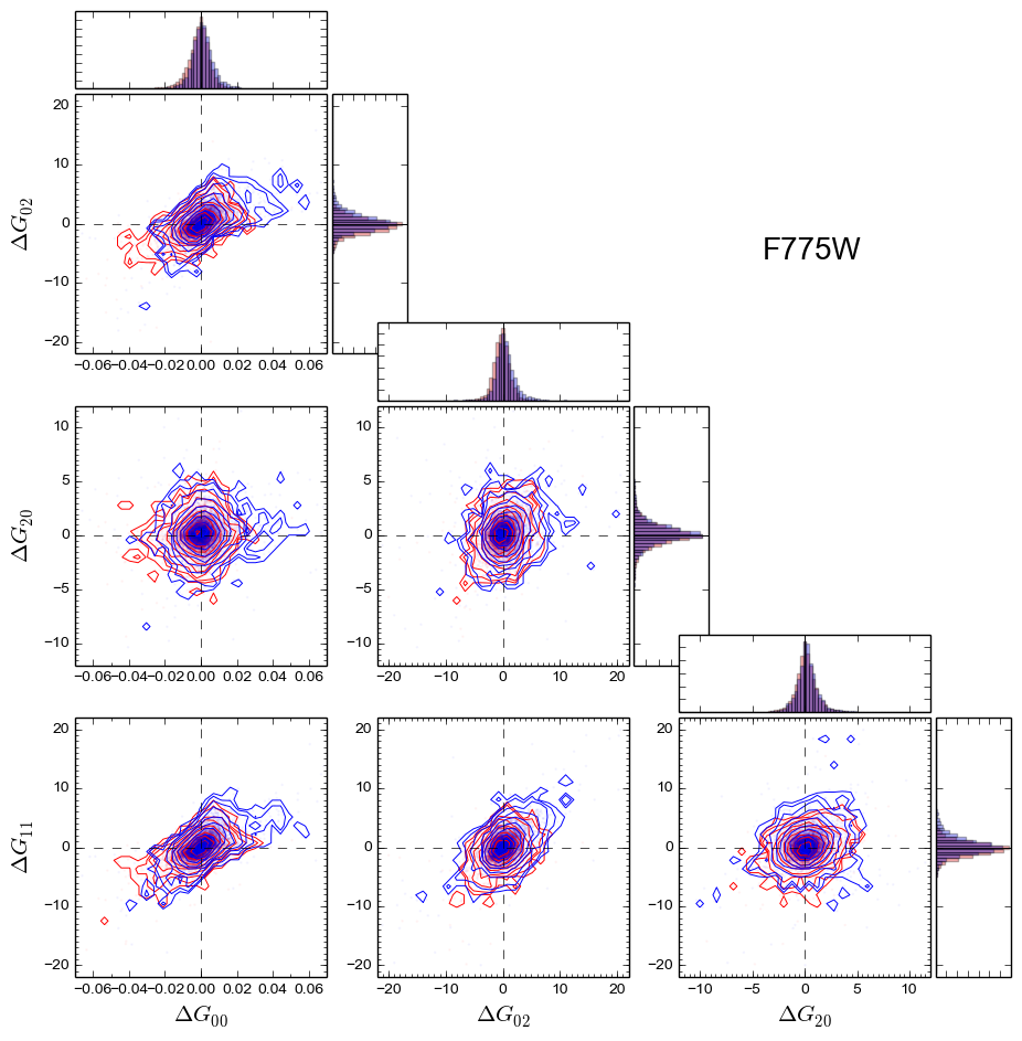
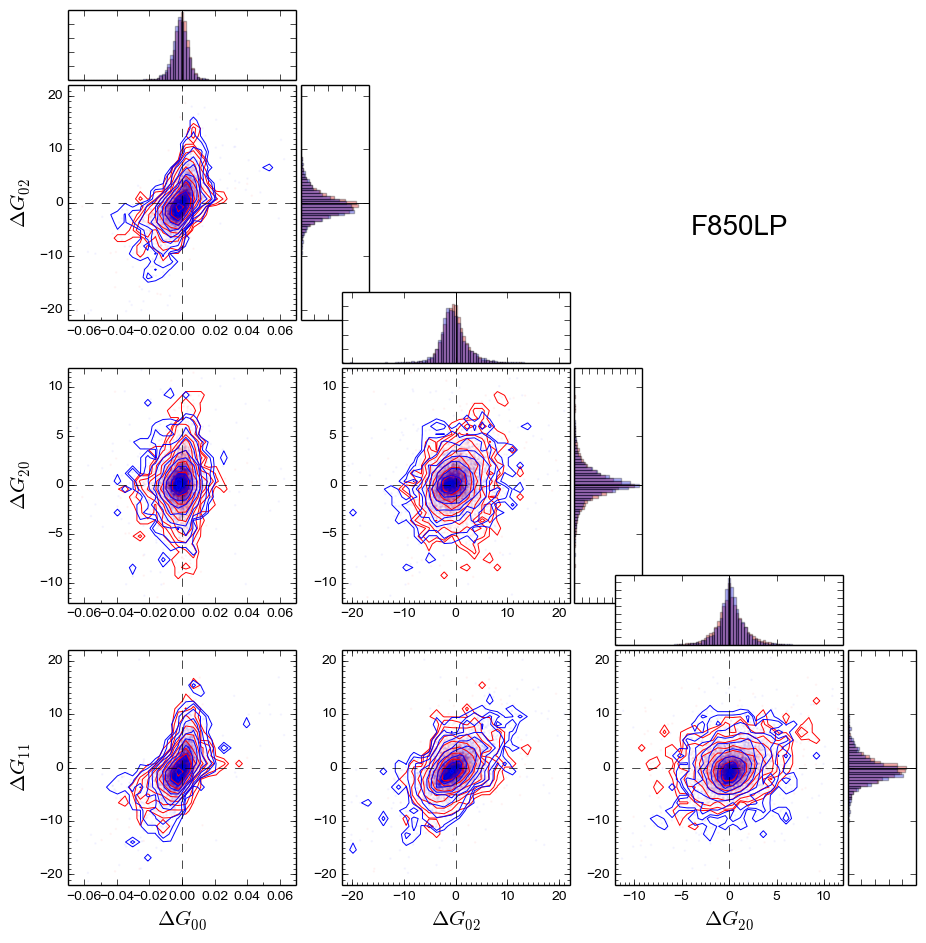
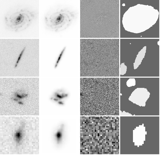
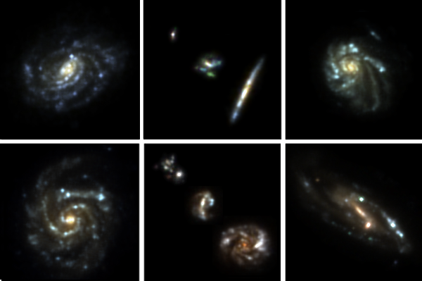
Figure (8) displays four galaxies belonging to the same four samples used to create the basis shown in Fig. (7). The images have been rescaled to better visualize their details. For each object we show, from left to right, the original image, the model, the residuals, and the segmentation used to remove nearby objects. The color images of the same galaxies are shown in the top left and central panels of Fig. (9) together with additional examples. The color stamps have a field size of $5.4$ arcsec, are based on the F435W, F606W, and F775W filters and show once more the range of sizes and morphologies which can be modeled. In this case, the galaxies are visualized without any rescaling. The residuals are compatible with the image noise except for very concentrated features which are slightly missed because of the regularization scheme we adopted when constructing the basis functions which the models are based on (see Fig. 8).

6 Testing the brightness moments

In this section, we “feed” EasySky with the postage-stamps of the galaxy models created in Sec. (5) and extracted from the XDF Survey with EasyEMPCA. In this case, the galaxies have been arranged on a regular grid, randomly flipped, and rotated by multiples of $90$ degrees. Their flux has not been changed to produce an image as close as possible to the original data. Such image permutations do not affect the original quality of the stamps because no interpolation is involved in this process, as it would happen when applying arbitrary rotations.

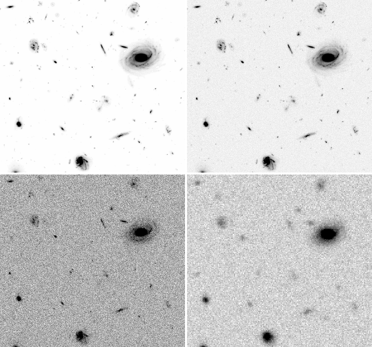
In Fig. (10), we show a realization of a portion of $0.65\times 0.65$ arcmin² field-of-view in the F755W band. The noise-free image is shown in the top left panel, while the other panels show three images with different levels of noise and resolution to resemble the XDF survey (upper right panel), one orbit exposure with HST (bottom left), and a CFHTLens stacked image with a seeing of $0.7$ arcsec (bottom right panel). We can now process these simulations like real images to verify and quantify the accuracy of the galaxy reconstructions. Do do so, we first detect the objects with SExtractor and then apply EasyPCA with the complete procedure to derive the basis and the models (see Sec. 2). It is important to note that even if the mock galaxies used in the simulations have been produced with the EMPCA, we took care to create a sample of galaxies which is as independent as possible from the original sample. This is why the galaxy images have been randomly flipped, rotated and split into training sets differing, in number and components, from the training set used to create the simulations in first place. Further more, the noise in the simulated images is not the same as that in the real data.

To have a quantitative assessment of the reconstruction quality, we measured the brightness moments,

$$G_{ij}=\int_{-\infty}^{\infty}d(\mn@boldsymbol{x})x_{1}^{i}x_{2}^{j}\mathrm{d}x\;,$$ (9)

of all galaxies in the simulation with noise to quantify the deviations with respect to those expected in the noise-free images. In Fig. (11), we plot the scatter in the brightness moments, $\Delta G_{ij}=G_{ij}^{measured}-G_{ij}^{true}$, up to the second order (as required for weak-lensing measurements). The moments except $G_{00}$ have been normalized by flux.

We finally processed the same images with a well-established weak-lensing method to have a direct comparison. At this end, we used the Shapelens library which allows to measure the brightness moments by iteratively matching the data to an elliptical weight function to maximize the signal-to-noise ratio (Melchior et al., 2011). The brightness moments of the models based on the EMPCA (blue contours) are reproduced with an accuracy comparable to that achieved by Shapelens (red contours), proving the quality of the models.

7 Conclusions

We have described how optical images of galaxies can be fitted with an optimized linear model based on the Expectation Maximization Principal Components Analysis (EMPCA). This method relies on the data alone, avoiding any assumptions regarding the morphology of the objects to be modeled even if they have complex or irregular shapes. As a test case, we have analyzed the galaxies listed in the Rafelski et al. (2015) catalog which covers the Hubble eXtreme Deep Field (XDF). We selected those objects with magnitude $m_{W755}<30$, far from the field edges and without overlapping artifacts caused by the few stars present across the field. We collected 7038 postage-stamps of noise-free galaxy images with redshift up to $z=4.0$.

We have shown how the modeled galaxies well represent the entire collection of galaxies, from small to large and from regular to irregular. Two codes have been implemented to this end: EasySky to create the simulations and EasyEMPCA to model the galaxies. The residuals appear uncorrelated except at very sharp features because of the regularization scheme we adopted during the basis construction. To further verify the quality of the reconstructions, we simulated a set of galaxy images, with and without noise, covering the entire spectrum of shapes and luminosities of the objects present in the XDF. We processed the simulations with the same procedure applied to a real data set: we detected the objects with SExtractor, derived the EMPCA basis and fitted the data with the linear model based on this basis. We then measured the brightness moments up to the second order of the model reconstructions and compared them to those of the noise-free simulations. The quality of the reconstructions very well competes with a well-established method to measure galaxy brightness moments such as the iterative adaptive scheme implemented in Shapelens.

The procedure discussed in this paper can be used to derive the properties of galaxies such as their fluxes and shapes, or to create reliable simulations of optical images. In this respect, the accuracy of such simulations is gaining importance for the lensing community. For instance, in the strong-lensing regime, they are necessary to understand how substructures in strongly magnified galaxies can be used to access additional information on the lensing mass distribution, such as galaxy clusters. In the weak-lensing regime, all methods to measure the ellipticites of galaxies require precise simulations for their calibration, on which depends the bias of such measurements and all quantities derived from them. The method we discussed in this work appears as a promising solution to create such simulations.

References

- Bailey (2012) Bailey S., 2012, PASP, 124, 1015
- Bartelmann et al. (2012) Bartelmann M., Viola M., Melchior P., Schäfer B. M., 2012, A&A, 547, A98
- Beltrando (1990) Beltrando G., 1990, J. Climatol., 10, 691
- Bertin & Arnouts (1996) Bertin E., Arnouts S., 1996, A&AS, 117, 393
- Bridle et al. (2010) Bridle S., et al., 2010, MNRAS, 405, 2044
- Bruderer et al. (2016) Bruderer C., Chang C., Refregier A., Amara A., Bergé J., Gamper L., 2016, ApJ, 817, 25
- Cattell (1966) Cattell R., 1966, Multiv. Behav. Res., 1, ,245
- Cattell & Vogelmann (1977) Cattell R., Vogelmann S., 1977, Mult. Behav. Res., 12, 289
- Ferré (1990) Ferré L., 1990, Preprint. Laboratoire de Statistique et Probabilit és
- Gurvich & Mandelbaum (2016) Gurvich A., Mandelbaum R., 2016, MNRAS, 457, 3522
- Heymans et al. (2006) Heymans C., et al., 2006, MNRAS, 368, 1323
- Illingworth et al. (2013) Illingworth G. D., et al., 2013, ApJS, 209, 6
- Jolliffe (2002) Jolliffe I., 2002, Principal Component Analysis. Springer Verlag
- Joseph et al. (2014) Joseph R., et al., 2014, A&A, 566, A63
- Kaiser et al. (2002) Kaiser N., et al., 2002, in Tyson J. A., Wolff S., eds, Proc. SPIEVol. 4836, Survey and Other Telescope Technologies and Discoveries. pp 154–164, doi:10.1117/12.457365
- Kitching et al. (2012) Kitching T. D., et al., 2012, MNRAS, 423, 3163
- Laureijs (2009) Laureijs R., 2009, preprint, (arXiv:0912.0914)
- Mandelbaum et al. (2015) Mandelbaum R., et al., 2015, MNRAS, 450, 2963
- Maryon (1979) Maryon R., 1979, Met O 13 Branch Memorandum, 13
- Massey et al. (2004) Massey R., Refregier A., Conselice C. J., David J., Bacon J., 2004, MNRAS, 348, 214
- Massey et al. (2007) Massey R., et al., 2007, MNRAS, 376, 13
- Massey et al. (2013) Massey R., et al., 2013, MNRAS, 429, 661
- Melchior & Viola (2012) Melchior P., Viola M., 2012, MNRAS, 424, 2757
- Melchior et al. (2011) Melchior P., Viola M., Schäfer B. M., Bartelmann M., 2011, MNRAS, 412, 1552
- Meneghetti et al. (2008) Meneghetti M., et al., 2008, A&A, 482, 403
- Moffat (1969) Moffat A. F. J., 1969, A&A, 3, 455
- Rafelski et al. (2015) Rafelski M., et al., 2015, AJ, 150, 31
- Refregier (2003) Refregier A., 2003, MNRAS, 338, 35
- Refregier & Bacon (2003) Refregier A., Bacon D., 2003, MNRAS, 338, 48
- Refregier et al. (2012) Refregier A., Kacprzak T., Amara A., Bridle S., Rowe B., 2012, MNRAS, 425, 1951
- Rowe et al. (2015) Rowe B. T. P., et al., 2015, Astronomy and Computing, 10, 121
- S.A. (1971) S.A. F., 1971, Statistician, 20, 63
- Sersic (1968) Sersic J. L., 1968, Atlas de galaxias australes. Observatorio Astronomico, Universidad Nacional de Cordoba
- Srebro & Jaakkola (2003) Srebro N., Jaakkola T., 2003, Proc. of the twentieth Intl Conf. on Machine Learning (Washington, DC: AAAI Press), 720, http://www.aaai.org/Press/Proceedings/icml03.php
- Viola et al. (2011) Viola M., Melchior P., Bartelmann M., 2011, MNRAS, 410, 2156
- Zitrin et al. (2015) Zitrin A., et al., 2015, ApJ, 801, 44