Kondo effect in a quantum wire with spin-orbit coupling

Abstract

The influence of spin-orbit interactions on the Kondo effect has been under debate recently. Studies conducted recently on a system composed by an Anderson impurity on a 2DEG with Rashba spin-orbit have been shown that it can enhance or suppress the Kondo temperature ($T_{\rm K}$), depending on the relative energy level position of the impurity with respect to the particle-hole symmetric point. Here we investigate a system composed by a single Anderson impurity side-coupled to a quantum wire with spin-orbit coupling (SOC). We derive an effective Hamiltonian in which the Kondo coupling is modified by the SOC. In addition, the Hamiltonian contains two other scattering terms, the so called Dzaloshinskyi-Moriya interaction, know to appear in these systems, and a new one describing processes similar to the Elliott-Yafet scattering mechanisms. By performing a renormalization group analysis on the effective Hamiltonian, we find that the correction on the Kondo coupling due to the SOC favors and enhancement of the Kondo temperature even in the particle-hole symmetric point of the Anderson model, agreeing with the NRG results. Moreover, away from the particle-hole symmetric point, $T_{\rm K}$ always increases with the SOC, accordingly with the previous renormalization group analysis.

I introduction

The well-known Kondo effect is a many-body dynamical screening of a localized magnetic moment by the spins of itinerant electrons that occurs at temperatures below the so called the Kondo temperature ($T_{\rm K}$).Hewson Originally observed in bulk magnetic alloysKondo with conspicuous transport features, this effect has been extensively studied in few magnetic impurities coupled to oneMadhavan ; Manoharan ; Crommie and twoGiordano ; Webb ; Iye dimensional systems. Recently, a number of studies has discussed the effect spin-orbit coupling (SOC) on the Kondo effect on two dimensional systems. More specifically, the question on how the SOC modifies the Kondo effect in systems with an isolated magnetic impurities has gained more attention.Malecki ; Zarea ; Zitko ; Diego ; Wong ; Isaev ; Avishai ; Andergassen The influence of the effect of SOC on the Kondo physics has gained major interest because the former has become remarkably attractive in condensed matter systems.Winkler ; Manchon For example, SOC is the basic ingredient for many different phenomena, extending from the spin manipulation in the celebrated Datta-Das transistorData-Das to the more fundamental physics as in the quantum spin-hall effectBernevig2 and Majorana Fermions.Read

Since the Kondo effect involves collectively the spins of the itinerant electrons, it is not surprising that SOC—that locks the electron spin with their momenta—will modify it. In fact, while in Ref. Malecki, it was found no change in the Kondo temperature with SOC, recent studiesZarea ; Zitko ; Diego ; Wong have found a change in the Kondo temperature Rashba SOC. Apart from the Ref. Diego, that addresses the Kondo effect in graphene, the other ones report arguable results about similar systems. On the one hand in Ref. Malecki, it was found that the Rashba SOC causes essentially no effect on $T_{\rm K}$. On the other, in Ref Zarea, , by renormalization group analysis (RGA) and in Refs. Zitko, and Wong, , using the numerical renormalization group (NRG), report $T_{\rm K}$ dependent on the SOC. Although, the actual functional dependency obtained by the NRG seems to differ from the RGA approach. This controversy can be attributed to the different regimes in which the analysis were carried out and to some approximations made in the RGA. We should stress that the Malecki’s idea of studying the effect of SOC on $T_{\rm K}$ using a standard Kondo model was incomplete. This became apparent in Ref. Zarea, , in which it was shown that the standard Kondo model does not include all the scattering phenomena in the system.

Figure 1: (Color online) Schematic representation of a quantum dot side-coupled to a quantum wire with spin-orbit interaction. The wire is assumed to lie along the $x$-direction. $V_{k}$ represents the hopping of electrons from the quantum into the wire.

Thanks to the various studies discussed above, the effect of SOC on the Kondo temperature in two-dimensional systems have been quite well elucidated. In one dimensional systems, however, the effect of the SOC in the Kondo effect may be even more important and has not been investigated so far. The expected importance of the SOC on the Kondo effect on 1D systems can be viewed in as simple way. As mentioned above, the Kondo effect is based on scatterings accompanied by spin-flip processes involving the spins of the conduction electrons and that one of the local magnetic moments. At very low temperature, energy conserving scatterings become more relevant as compared to non-conserving ones. Contrasting with the 2D case, in which energy conserving skew scatterings are also allowed, in 1D only forward or backward scattering can occur. In situations in which a backward scattering events suffered by the conduction electrons requires a flip of their spins, it is expectable that the SOC have a much stronger influence in the Kondo effect in 1D systems as compared to the 2D ones. Such a spin-momentum locking is known to occur in strongly spin-orbit coupled 1D system, such as InSb nanowiresWimmer and in 1D edge state of topological insulators.Hasan

Motivated by the aforementioned peculiarities of the SOC in one-dimensional systems, we investigate the Kondo effect of a magnetic impurity side-coupled to a quantum wire with both RashbaRashba and DresselhausDresselhaus SOC. For the impurity, we restrict ourselves to a spin-1/2 magnetic moment and model it as a single level interacting quantum dot that couples to the conduction electrons in the quantum wire through tunneling matrix elements. By projecting the total Hamiltonian of the system onto a singly occupied subspace of the impurity we derive an effective Kondo Hamiltonian, which contains the know Dzyaloshinskii-Moriya interaction terms and an additional term, analogous to the Elliott-Yafet spin-flip scattering mechanism induced by the SOC.Elliott ; Yafet ; Fert ; Batley Once we have obtained our effective Kondo-like Hamiltonian, we perform a renormalization group analysis (similarly to what was done in Ref. Zarea, ) from which we extract the Kondo temperature.

Our results show that the dependence of $T_{\rm K}$ with the SOC strength differs from what was found in Ref. Zarea, . For instance, we find that the Kondo temperature always increases, even when the system is at the particle-hole symmetric point, that contrats with the results reported in Ref. Zarea, but agree with those found in Refs Zitko, and Wong, . The disagreement between our results and those of Ref. Zarea, is attributed to the correction on the effective Kondo coupling due to the SO interaction, neglected in the previous study. It is also noteworthy that the dependence of $T_{\rm K}$ with the SO coupling is particle-hole asymmetric. We show that an extra scattering term in the effective Hamiltonian is the one responsible for breaking the particle-hole symmetry of the RG equation.

The remainder of this paper is organized as follows: In Sec. II we present the model Hamiltonian and derive an effective Kondo-like Hamiltonian and in Sec. III we perform a renormalization group analysis with numerical solution. Finaly, in Sec. IV we summarize our mains results. Some of the details of the calculations are shown in the appendices.

II Hamiltonian model

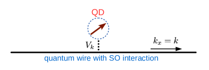
For the sake of clarity, we schematically represent our system in Fig. 1, in which the local magnetic moment is modeled by a sigle-level quantum dot occupied by one electron. The quantum wire is assumed to lie along the $x$-axis and includes both RashbaRashba and linear Dresselhaus SOC.Dresselhaus Because of the dimensionality of the wire, both SOCs are treated in the same footing. More formally, our system is described by an Anderson-like model, $H=H_{\mathrm{wire}}+H_{\mathrm{dot}}+H_{\mathrm{dot-wire}}$, where

$$H_{\mathrm{dot}}=\sum_{s}\varepsilon_{d}d_{s}^{{\dagger}}d_{s}+Un_{\uparrow}n_{\downarrow},$$ (1)

describes the isolated quantum dot, in which $d^{\dagger}_{s}$ ($d_{s}$) creates (annihilates) an electron with energy $\varepsilon_{d}$ and spin $s$ in the dot and $U$ is the on-site Coulomb repulsion in the quantum dot. We also have defined the number operator $n_{s}=d^{\dagger}_{s}d_{s}$. The quantum wire is described by

$$H_{\mathrm{wire}}=\sum_{k}\left[\varepsilon_{k}\delta_{ss^{\prime}}+k\left(\beta\sigma^{x}_{ss^{\prime}}-\alpha\sigma^{y}_{ss^{\prime}}\right)\right]c^{\dagger}_{ks}c_{ks^{\prime}},$$ (2)

where $k$ is the momentum along $x$-axis, $\varepsilon_{k}={\hbar^{2}k^{2}}/{2m^{*}}$ the kinetic energy with $m^{*}$ representing the effective mass of the conduction electrons. The operator $c^{\dagger}_{ks}$ ($c_{ks}$) creates (annihilates) an electron with momentum $k$ and spin $s$ in the wire. The Rashba and the linear Dresselhaus spin-orbit interaction coupling is parametrized by the interaction strength $\alpha$ and $\beta$, respectively, and $\sigma^{\nu}$ (with $\nu=x,y,z$) represents the Pauli matrices. Finally,

$$H_{\mathrm{dot-wire}}=\sum_{ks}\left(V_{k}c_{ks}^{{\dagger}}d_{s}+V_{k}^{*}d_{s}^{{\dagger}}c_{ks}\right)$$ (3)

couples the quantum dot to the wire with overlap matrix element $V_{k}$.

We should keep in mind that we aim to deriving an effective Kondo-like Hamiltonian by projecting out the empty and the doubly occupied states of the quantum dot. Before doing so, we want to bring the full Hamiltonian into the the single impurity Anderson model (SIAM) form. To accomplished this, we diagonalize $H_{\mathrm{wire}}$ by performing the following rotation in the spin space,

$$\begin{pmatrix}c_{k+}\\ c_{k-}\end{pmatrix}={\mathcal{U}}\begin{pmatrix}c_{k\uparrow}\\ c_{k\downarrow}\end{pmatrix},$$ (4)

with

$${\mathcal{U}}=\frac{1}{\sqrt{2}}\begin{pmatrix}1&e^{-i\theta}\\ -ie^{i\theta}&i\end{pmatrix},$$ (5)

where $\theta=\tan^{-1}(\beta/\alpha)$. Under this transformation, the Hamiltonian $H_{\mathrm{wire}}$ acquires the diagonal form

$$\tilde{H}_{\mathrm{wire}}=\sum_{kh}\varepsilon_{kh}c^{\dagger}_{kh}c_{kh},$$ (6)

in which $h=+,-$ is the helical quantum number and $\varepsilon_{kh}=\hbar k^{2}/2m^{*}+h|\gamma|k$ with $\gamma=\alpha-i\beta$. By applying the same transformation to the quantum dot operators we see that the form of $H_{\mathrm{dot}}$ and $H_{\mathrm{dot-wire}}$ remain unchanged. Therefore, in the SO basis, the total Hamiltonian acquires the SIAM form

$$\tilde{H}=\sum_{h}\varepsilon_{d}d_{h}^{{\dagger}}d_{h}+Un_{+}n_{-}+\sum_{kh}\varepsilon_{kh}c^{\dagger}_{kh}c_{kh}$$

$$+\sum_{kh}\left(V_{k}c_{kh}^{{\dagger}}d_{h}+V^{*}_{k}d^{\dagger}_{h}c_{kh}\right),$$

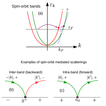
where $\varepsilon_{kh}=\varepsilon_{k}+h|\gamma|k$. These are the SO bands shown in Fig. (2)(a). We are now ready to derive the effective Kondo-like Hamiltonian.

II.1 The effective Hamiltonian

Since we are interested in the Kondo regime of the system in which there is a magnetic moment localized in the quantum dot, we project the Hamiltonian (II) onto the singly occupied subspace of the quantum dot Hilbert space. We follow the same strategy described in Hewson’s bookHewson (for details, see the Appendix A). The resulting effective Hamiltonian can be written in the form

$$H_{\rm eff}=H_{0}+H_{\rm K}+H_{\rm DM}+H_{\rm EY}.$$ (8)

Here,

$$H_{0}=\sum_{k,h}\varepsilon_{kh}c^{\dagger}_{kh}c_{kh}$$ (9)

describes the conduction band on the SO basis,

$$H_{\rm K}=\sum_{kk^{\prime}}J_{kk^{\prime}}\left[\left(c^{\dagger}_{k^{\prime}+}c_{k+}-c^{\dagger}_{k^{\prime}-}c_{k-}\right)S_{z}+c^{\dagger}_{k^{\prime}+}c_{k-}S_{-}+c^{\dagger}_{k^{\prime}-}c_{k+}S_{+}\right]$$

describes the Kondo coupling, in which

$$J_{kk^{\prime}} = V_{k}V^{*}_{k^{\prime}}\frac{A_{k}+A_{k^{\prime}}}{2},$$ (11)

with

$$A_{k}=\frac{\varepsilon_{k}-\varepsilon_{d}}{(\varepsilon_{k}-\varepsilon_{d})^{2}-|\gamma|^{2}k^{2}}+\frac{\varepsilon_{d}+U-\varepsilon_{k}}{(\varepsilon_{d}+U-\varepsilon_{k})^{2}-|\gamma|^{2}k^{2}}.$$ (12)

Observe that $J_{kk^{\prime}}$ depends on the SO coupling $\gamma$. By inspection we see in the absence of the spin-orbit interaction ($\gamma=0$) we recover the conventional Kondo coupling, for which $A_{k}=(\varepsilon_{d}+U-\varepsilon_{k})^{-1}+(\varepsilon_{k}-\varepsilon_{d})^{-1}$.

The last two terms of the Hamiltonian (8) are given by

$$H_{\rm DM}=\sum_{kk^{\prime}}\Gamma_{kk^{\prime}}\left(c^{\dagger}_{k^{\prime}+}c_{k-}S_{-}-c^{\dagger}_{k^{\prime}-}c_{k+}S_{+}\right),$$ (13)

and

$$H_{\rm EY}=H_{\rm EY}^{(1)}+H_{\rm EY}^{(2)}.$$ (14)

In this last expression,

$$H^{(1)}_{\rm EY}=\sum_{kk^{\prime}}\Gamma^{(1)}_{kk^{\prime}}(c^{\dagger}_{k^{\prime}+}c_{k+}+c^{\dagger}_{k^{\prime}-}c_{k-})S_{z},$$

and

$$H^{(2)}_{\rm EY}=\sum_{kk^{\prime}}\Gamma^{(2)}_{kk^{\prime}}\frac{n_{d}}{2}(c^{\dagger}_{k^{\prime}+}c_{k+}-c^{\dagger}_{k^{\prime}-}c_{k-}).$$ (16)

The couplings in the Eqs. (13), (II.1) and (16) can be written as

$$\Gamma_{kk^{\prime}}=V_{k}V^{*}_{k^{\prime}}\frac{B^{(+)}_{k}-B^{(+)}_{k^{\prime}}}{2},$$ (17)

$$\Gamma^{(1)}_{kk^{\prime}}=V_{k}V^{*}_{k^{\prime}}\frac{B^{(+)}_{k}+B^{(+)}_{k^{\prime}}}{2},$$ (18)

and

$$\Gamma^{(2)}_{kk^{\prime}}=V_{k}V^{*}_{k^{\prime}}\frac{B^{(-)}_{k}+B^{(-)}_{k^{\prime}}}{2}.$$ (19)

Here we have defined

$$B^{(\pm)}_{k}=\pm|\gamma|k\left[\frac{1}{(\varepsilon_{k}-\varepsilon_{d})^{2}-|\gamma|^{2}k^{2}}\mp\frac{1}{(\varepsilon_{d}+U-\varepsilon_{k})^{2}-|\gamma|^{2}k^{2}}\right].$$

The Hamiltonian (13) corresponds to the known Dzyaloshinskii-Moriya interaction while (II.1) and (16) describe the Elliott-Yafet like processes,Elliott ; Yafet responsible for spin-flip scatterings of the conduction electrons by the localized magnetic moments.Wernick The spin-flip processes involved in the Hamiltonian (II.1) and (16) are not apparent in the SO basis but is clearly seen when these Hamiltonians are written in the real spin representation (see Appendix B).

Figure 2: (Color online) (a) Spin-orbit bands for the conduction electrons. At low temperature, the allowed processes are those involving energies close to the Fermi level $\varepsilon_{F}$. The magenta and purple arrows exemplify, respectively, the intra-band (forward) and intra-band (backward) scatterings. The panels (b) and (c) are representative scattering diagrams describing typical processes that contained in the Hamiltonians (II.1) and (30), respectively.

At low temperature regime we can assume that the scatterings occurs only for electrons with momenta close to Fermi momentum, $k_{F}$. Moreover, for small SO interaction, such that $|\gamma|k_{F}\ll\hbar k_{F}^{2}/2m^{*}$ (or $|\gamma|\ll\hbar k_{F}/2m^{*}$), we can set $\varepsilon_{k}\approx\varepsilon_{k_{F}}=0$ and $V_{k}=V_{k_{F}}\equiv V$. With this we can make the approximations

$$J_{kk^{\prime}} \approx |V|^{2}\left[\frac{\varepsilon_{d}+U}{(\varepsilon_{d}+U)^{2}-|\gamma_{F}|^{2}}-\frac{\varepsilon_{d}}{\varepsilon_{d}^{2}-|\gamma_{F}|^{2}}\right]\equiv J,$$ (21)

$$\Gamma_{kk^{\prime}} \approx |V|^{2}|\gamma|\frac{k-k^{\prime}}{2}\left[\frac{1}{\varepsilon_{d}^{2}-|\gamma_{F}|^{2}}-\frac{1}{(\varepsilon_{d}+U-\varepsilon_{k})^{2}-|\gamma_{F}|^{2}}\right],$$

$$\Gamma^{(1)}_{kk^{\prime}} \approx |V|^{2}|\gamma|\frac{k+k^{\prime}}{2}\left[\frac{1}{\varepsilon_{d}^{2}-|\gamma_{F}|^{2}}-\frac{1}{(\varepsilon_{d}+U-\varepsilon_{k})^{2}-|\gamma_{F}|^{2}}\right],$$

and

$${\Gamma}^{(2)}_{kk^{\prime}} \approx -|V|^{2}|\gamma|\frac{(k+k^{\prime})}{2}\left[\frac{1}{\varepsilon_{d}^{2}-|\gamma_{F}|^{2}}+\frac{1}{(\varepsilon_{d}+U-\varepsilon_{k})^{2}-|\gamma_{F}|^{2}}\right].$$

In the equations above we have define $\gamma_{F}=\gamma k_{F}$. To obtain the expressions (21)-(II.1) we have replaced $k^{2}$ and $k^{\prime 2}$ by $k_{F}^{2}$ but we were careful with the linear terms, keeping $k$ and $k^{\prime}$ intact. This is because the sums in the Hamiltonian above run for positive and negative momenta. Therefore, considering only scatterings around $k_{F}$ we can replace $|k|$ and $|k^{\prime}|$ by $k_{F}$ in the couplings (II.1)-(II.1). With this, the factor $k-k^{\prime}$ in the Eq. (II.1) or $k+k^{\prime}$ in Eqs. (II.1) and (II.1) can be approximated by zero or $\pm 2k_{F}$, depending on the relative sign between $k$ and $k^{\prime}$. Bearing this in mind, we see that the coupling (II.1) contributes only with backward scatterings whereas the Eqs. (II.1) and (II.1) contribute only with forward scatterings. Explicitly, at $k_{F}$ we can write

$$\Gamma=V|^{2}\gamma_{F}\left[\frac{1}{\varepsilon_{d}^{2}-|\gamma_{F}|^{2}}-\frac{1}{(\varepsilon_{d}+U)^{2}-|\gamma_{F}|^{2}}\right]=-\Gamma_{1},$$ (25)

and

$$\Gamma_{2}=-|V|^{2}\gamma_{F}\left[\frac{1}{\varepsilon_{d}^{2}-|\gamma_{F}|^{2}}+\frac{1}{(\varepsilon_{d}+U)^{2}-|\gamma_{F}|^{2}}\right].$$ (26)

Inserting these expressions into Eqs. (II.1), (13), (II.1), and (16) we obtain

$$H_{\rm K}=J\sum_{kk^{\prime}}\left[\left(c^{\dagger}_{k^{\prime}+}c_{k+}-c^{\dagger}_{k^{\prime}-}c_{k-}\right)S_{z}+c^{\dagger}_{k^{\prime}+}c_{k-}S_{-}+c^{\dagger}_{k^{\prime}-}c_{k+}S_{+}\right],$$

$$H_{\rm DM}=\Gamma\sum_{kk^{\prime}>0}\left(c^{\dagger}_{-k^{\prime}+}c_{k-}S_{-}-c^{\dagger}_{k^{\prime}+}c_{-k-}S_{-}+c^{\dagger}_{k^{\prime}-}c_{-k+}S_{+}\right.$$

$$-\left.c^{\dagger}_{-k^{\prime}-}c_{k+}S_{+}\right),\quad$$ (28)

$$H_{\rm EY}^{(1)} = \Gamma_{1}\sum_{kk^{\prime}>0}\left[S_{z}(c_{k^{\prime}+}^{{\dagger}}c_{k+}-c_{-k^{\prime}+}^{{\dagger}}c_{-k+})\right.$$ (29)

$$\qquad\qquad\qquad\left.+S_{z}(c_{k^{\prime}-}^{{\dagger}}c_{k-}-c_{-k^{\prime}-}^{{\dagger}}c_{-k-})\right]$$

$$H_{EY}^{(2)} = \Gamma_{2}\sum_{kk^{\prime}>0}\left[\frac{n_{d}}{2}(c_{k^{\prime}+}^{{\dagger}}c_{k+}-c_{k^{\prime}-}^{{\dagger}}c_{k-})\right.$$ (30)

$$\qquad\qquad\qquad\left.+\frac{n_{d}}{2}(c_{-k^{\prime}-}^{{\dagger}}c_{-k-}-c_{-k^{\prime}+}^{{\dagger}}c_{-k+})\right].$$

Note that it is now explicit that the processes in the Hamiltonians $H_{\rm DM}$ and in $H_{\rm EY}$ involve only backward and forward scatterings, respectively. Moreover, we see that the backward scatterings occur are inter-band while the forward ones are intra-band scatterings. These backward (inter-band) and forward (intra-band) scatterings are exemplified with the diagrams of Fig. 2(b) and 2(c). Because of this very well defined scattering processes, it is convenient to split the Kondo, likewise. Separating the terms of (II.1) involving definite backward and forward processes as

$$H_{\rm K} = J^{\rm F}_{\parallel}\sum_{kk^{\prime}>0\atop kk^{\prime}<0}\left(c^{\dagger}_{k^{\prime}+}c_{k+}-c^{\dagger}_{k^{\prime}-}c_{k-}\right)S_{z}$$ (31)

$$+J^{\rm B}_{\parallel}\sum_{k>0,k^{\prime}<0\atop k<0,k^{\prime}>0}\left(c^{\dagger}_{k^{\prime}+}c_{k+}-c^{\dagger}_{k^{\prime}-}c_{k-}\right)S_{z}$$

$$+J^{\rm F}_{\perp}\sum_{kk^{\prime}>0\atop kk^{\prime}<0}\left[c^{\dagger}_{k^{\prime}+}c_{k-}S_{-}+c^{\dagger}_{k^{\prime}-}c_{k+}S_{+}\right]$$

$$+J^{\rm B}_{\perp}\sum_{k>0,k^{\prime}<0\atop k<0,k^{\prime}>0}\left[c^{\dagger}_{k^{\prime}+}c_{k-}S_{-}+c^{\dagger}_{k^{\prime}-}c_{k+}S_{+}\right].$$

As we will see below, because of the SOC, the several Kondo couplings in the Eq. (31) will obey different differential equation in the renormalization group analysis.

III Renormalization group analysis

To study the low-temperature regime of the system we perform a poor-man scaling analysis of the effective Hamiltonian (8). We follow the original Anderson’s approachAnderson to obtain the renormalization equations for the effective couplings. After a cumbersome but straightforward calculation (see Appendix C) we find

$$\dot{J}_{\perp B} = -\rho J_{\perp F}J_{\parallel B}-\rho J_{\perp B}J_{\parallel F}+\rho\Gamma\Gamma_{1}-\rho\Gamma\Gamma_{2}$$ (32a)

$$\dot{J}_{\perp F} = -\rho J_{\perp F}J_{\parallel F}-\rho J_{\perp B}J_{\parallel B}$$ (32b)

$$\dot{J}_{\parallel B} = -2\rho J_{\perp F}J_{\perp B}$$ (32c)

$$\dot{J}_{\parallel F} = -\rho J_{\perp F}^{2}-\rho J_{\perp B}^{2}-\rho\Gamma^{2}$$ (32d)

$$\dot{\Gamma} = -\rho J_{\parallel F}\Gamma+\rho J_{\perp B}\Gamma_{1}-\rho J_{\perp B}\Gamma_{2}$$ (32e)

$$\dot{\Gamma}_{1} = \rho J_{\perp B}\Gamma+\rho J_{\parallel F}\Gamma_{2}$$ (32f)

$$\dot{\Gamma}_{2} = \rho J_{\parallel F}\Gamma_{1}.$$ (32g)

Following standard notation, in the equations above we have defined $\dot{X}\equiv dX/d\ln\Lambda$, where $\Lambda$ in the reduced bandwidth. We have also denoted $\rho=\rho(0)$ as the density of states of the conduction electrons calculated and the Fermi level, $\varepsilon_{F}=0$. For this we had to assume that the Fermi level is far away above the bottom of the band. In this limit we can linearize the band about $k=k_{F}$ as schematically shown in Fig (2)(a). We can verify that in the absence of SO interaction we have the solution for $\Gamma=\Gamma_{1}=\Gamma_{2}=0$, provided the condition has $\Gamma(D)=\Gamma_{1}(D)=\Gamma_{2}(D)=0$. With this, by setting $J_{\perp F}=J_{\parallel F}=J_{\perp B}=J_{\parallel B}=J$, the differential equations above reduce to the usual renormalization equation for $J$ in the isotropic Kondo model, $\dot{J}=-2\rho J^{2}$, leading to the known expression for the Kondo temperature, $T_{\rm K}^{0}=D{\rm Exp}(-1/2\rho J)$.

In the presence of SO interaction, an analytical solution for the coupled equations (32) is not available. Fortunately, it can be solved numerically using standard procedures. The numerical solution provides us with the coupling as a function of the reduced bandwidth $\Lambda$. As in the conventional Kondo model, the Kondo couplings diverge as $\Lambda\rightarrow 0$. It is precisely this divergence that provides a definition for the Kondo temperature within the renormalization group analysis. Using the same idea here, in the presence of the SO interaction, we take as $T_{\rm K}$ the value of $\Lambda$ where the numerical solution diverges.

Figure 3: (Color online) (a) Scaled Kondo temperature vs $\gamma_{F}/U$ for different values of $\varepsilon_{d}$ and $U=0.1$. $\varepsilon_{d}=-0.5U$ corresponds exactly to the particle-hole symmetric point of the Anderson model. Note the different behavior of $T_{\rm K}$ for $\varepsilon_{d}$ above and below $0.05$. $T_{\rm K}^{0}$ is the Kondo temperature calculated in the absence of the SO interaction, $\gamma=0$. (b) ${\rm Log}(T_{\rm K}/T_{\rm K}^{0})$ vs $\gamma_{F}/U$ (symbols). The Solid lines show straight lines connecting the first and the last points of each data set, serving as a guide to the eyes. These lines suggest that $T_{K}$ depends on $\gamma_{F}$ exponentially as $T_{\rm K}=T_{\rm K}^{0}\exp{(a\gamma_{F}^{2})}$, in which $a$ is a function of $\varepsilon_{d}$. (c) $a/U^{2}$ vs $\varepsilon_{d}/U$ extracted from the results of panel (b).

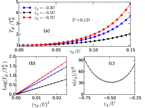
To obtain our results for $T_{\rm K}$, we set $U/\Delta=20$, with $\Delta=\pi V^{2}/2D$. Here, $D$ is an energy cutoff, within which the band is linearized around $k=k_{F}$. In Fig. 3(a) we show the Kondo temperature $T_{\rm K}/T_{\rm K}^{0}$ vs $\gamma_{F}/U$ for three different values of $\varepsilon_{d}$. Here $T_{\rm K}^{0}$ is the Kondo temperature in the absence of the SO interaction. Note that, similarly to what was obtained in Ref. Zarea, , $T_{\rm K}$ always increases with $\gamma_{F}$, but it is more pronounced for $\varepsilon_{d}\neq-U/2$ [squares (blue) and diamonds (red) curves]. The increase of $T_{\rm K}$ with $\gamma_{F}$ for $\varepsilon_{d}=-U/2$ contrasts with the results Ref. Zarea, that predicts a constant $T_{\rm K}$ using the same approach but agrees with those obtained in Refs,Zitko, ; Liang_Chen, ; Wong, . The main reason for the disagreement with the previous RGA is because they neglected corrections of the Kondo coupling $J$ due to the SO interaction. Another compelling point is that for $\varepsilon_{d}=-0.7U$ and $\varepsilon_{d}=-0.3U$ for which the impurity level is placed symmetrically below and above the particle-hole point, respectively, the increasing of $T_{\rm K}$ with $\gamma_{F}$ is not symmetric. This behavior disagree with those of Ref. Zarea, . This asymmetry is, however, quite different from asymmetry observed in the results of Refs. Zitko, ; Liang_Chen, ; Wong, because while they considered the Fermi level close to the bottom of the conduction band, here we assume $\varepsilon_{F}$ far away from it.

In the absence of analytical solution for the set of differential equations (32) we attempt to obtain qualitatively the dependence of $T_{\rm K}$ on $\gamma_{F}$. To do so, in Fig. 3(b) we plot ${\rm Log}(T_{\rm K}/T_{\rm K}^{0})$ vs $(\gamma_{G}/U)^{2}$ for the same three different values of $\varepsilon_{d}$ as in Fig. 3(a). The symbols correspond the numerical results as shown in 3(a) while the solid lines correspond to straight lines connecting the first and the last point of the data. Notably, these linear functions fit quite well all the data. This suggests a dependence of $T_{\rm K}$ on $\gamma_{F}$ as $T_{\rm K}=T_{\rm K}^{0}\exp{(a\gamma_{F}^{2})}$, where $a$ is a positive function of the Anderson model parameters (e. g. $\Delta,U,\varepsilon_{d}$). Here, by keeping all the other parameters fixed, $a$ clearly shows a strong dependence on $\varepsilon_{d}$. To extract a qualitative dependency of $a$ varies with $\varepsilon_{d}$, in Fig. 3(c) we plot $a$ vs $\varepsilon_{d}/U$. Note that the shape of the curve is almost parabolic with a minimum close to the particle-hole symmetry. It is, However, asymmetric about $\varepsilon_{d}=-U/2$ because of the particle-hole asymmetry of the renormalization equation introduced by the term $H_{\rm EY}^{(2)}$ of the effective Hamiltonian.

For a better comprehension of the origin of the particle-hole asymmetry in the results of Fig. 3 let us take a closer look at the renormalization equations (32). We will show that, in fact, the term in the Hamiltonian that breaks particle-hole symmetry of the renormalization equations is $H_{\rm EY}^{(2)}$, given by the Eq. (30). To this end, let us neglect $H_{\rm EY}^{(2)}$ in the renormalization equations Eqs. (32). We then remove the Eq. (32g) and make $\Gamma_{2}=0$ in all the other equations of the set (32). Now, remember that $\Gamma$ and $\Gamma_{1}$ are odd functions of $\varepsilon_{d}$ under the change $\varepsilon_{d}=-U/2+\delta$ to $\varepsilon_{d}=-U/2-\delta$ for any $\delta<U/2$. Therefore, for a given equal initial conditions for $J$’s (which is the case, since $J$ is even) we see that by changing $\varepsilon_{d}=-U/2+\delta$ to $\varepsilon_{d}=-U/2-\delta$ the derivative of both $\Gamma$ and $\Gamma_{1}$ just change their signs. Now, because the derivatives of the $J$’s depends on the product $\Gamma\Gamma_{1}$ or on $\Gamma^{2}$, which are both even, the resulting value of $T_{\rm K}$ extracted from the solution of the Eqs. (32) is particle-hole symmetric, even though $\Gamma$ and $\Gamma_{1}$ are odd. This show that indeed it is the additional term $H^{(2)}_{\rm EY}$ that breaks the particle-hole symmetry of the renormalization equations.

IV Conclusions

Summarizing, we have studied the influence of the Kondo effect of a magnetic impurity side coupled to a quantum wire with spin-orbit interaction. We start by modeling the system with a single impurity Anderson model (SIAM), in which the conduction electrons move under both Rashba and Dresselhaus spin-orbit couplings. We then derive an effective Kondo model that contains the known Dzaloshinskyi-Moriya (DM) interaction and an additional term describing scattering processes of the same type of the Elliott-Yafet (EY) mechanisms responsible for spin relaxation in systems with magnetic impurities. We splitting the total effective 1D Hamiltonian into forward and backward scattering we are able to obtain and then perform a poor-mans scaling to set of renormalization equations for the effective couplings. To obtain a Kondo temperature dependent of the SO coupling strength we solve numerically the coupled equations. We find that the spin-orbit interaction modifies, substantially, the Kondo temperature of the system. Our results show that, even though the DM term vanishes at the particle-hole (ph) symmetry of the SIAM, and is known to change the Kondo temperature only away from the ph symmetry, our study shows that the SOC modifies the Kondo temperature even in the ph symmetry since it modifies the conventional Kondo couplings. Moreover, we find that the contribution from additional EY to the enhancement of the Kondo temperature is asymmetric with respect to the ph symmetry. Our study shows clearly the scattering mechanisms of the conduction electrons by the magnetic impurity introduced by the SOC in the 1D system. More, importantly, we shown how these mechanism change the Kondo temperature of the system. We believe this work provides a step forward in the comprehension of the influence of SOC in the Kondo effect and is important for future studies, specifically in 1D systems.

Appendix A Derivation of the effective Hamiltonian

In order to project the total Hamiltonian (II) onto the singly occupied impurity subspace, we define the projector operators

$$P_{0} = (1-d^{\dagger}_{\uparrow}d_{\uparrow})(1-d^{\dagger}_{\downarrow}d_{\downarrow}),$$ (33)

$$P_{1} = d^{\dagger}_{\uparrow}d_{\uparrow}+d^{\dagger}_{\downarrow}d_{\downarrow}-2d^{\dagger}_{\uparrow}d^{\dagger}_{\downarrow}d_{\downarrow}d_{\uparrow},$$ (34)

$$P_{2} = d^{\dagger}_{\uparrow}d^{\dagger}_{\downarrow}d_{\downarrow}d_{\uparrow}.$$ (35)

The projected Hamiltonian can be written as

$$\!H_{\rm eff}\!=\!H_{11}\!+\!H_{10}\left(E\!-\!H_{11}\right)^{-1}\!H_{01}\!+\!H_{12}\left(E\!-\!H_{22}\right)^{-1}\!H_{21},$$ (36)

where $H_{ij}=P_{i}HP_{j}$. More explicitly, in terms of the creation and annihilation operators, the Hamiltonian (36) can be written as

$$H = H_{0}+\sum_{kk^{\prime}\atop hh^{\prime}}\frac{V_{k^{\prime}}^{*}V_{k}}{2}\Big{\{}\left[G_{h}(\varepsilon_{d},\varepsilon_{k})+G_{h^{\prime}}(\varepsilon_{d},\varepsilon_{k^{\prime}})\right]d_{\bar{h}}d^{\dagger}_{\bar{h}}d_{\bar{h}^{\prime}}d^{\dagger}_{\bar{h}^{\prime}}d^{\dagger}_{h}d_{h^{\prime}}c_{kh}c^{\dagger}_{k^{\prime}h^{\prime}}-\left[G_{h}(\varepsilon_{d}+U,\varepsilon_{k})+G_{h^{\prime}}(\varepsilon_{d}+U,\varepsilon_{k^{\prime}})\right]n_{d\bar{h}^{\prime}}c^{\dagger}_{k^{\prime}h^{\prime}}d_{h^{\prime}}n_{d\bar{h}^{\prime}}d^{\dagger}_{h}c_{kh}\Big{\}},$$

where

$$G_{h}(\varepsilon_{d},\varepsilon_{k})=\frac{1}{\varepsilon_{d}-\varepsilon_{k}}\left[1-\frac{h|\gamma|k}{\varepsilon_{d}-\varepsilon_{k}}\right]^{-1}.$$ (38)

In order to perform the summation on $h$ and $h^{\prime}$ in the Eq. (38) we expand the expression above as a power series of $x=h|\gamma|k(\varepsilon_{d}-\varepsilon_{k})^{-1}$. Summing up the infinite terms of the series we can write

$$G_{h}(\varepsilon_{d},\varepsilon_{k})\! = \!\frac{\varepsilon_{d}-\varepsilon_{k}}{(\varepsilon_{d}-\varepsilon_{k})^{2}-|\gamma|^{2}k^{2}}+\frac{h|\gamma|k}{(\varepsilon_{d}-\varepsilon_{k})^{2}-|\gamma|^{2}k^{2}}$$ (39)

$$= G^{(\rm e)}(\varepsilon_{d},\varepsilon_{k})+hG^{(\rm o)}(\varepsilon_{d},\varepsilon_{k})$$

where the first term corresponds to the even order of the series and the second on corresponds to the odd terms. We also have used the fact that $h^{j}=1$ for $j$ even and $h^{j}=h$ for $j$ odd. It is important to note that the series converges only for $|\gamma|k<(\varepsilon_{d}-\varepsilon_{k})$. This naturally imposes the regime of validity of the expansion, $|\gamma|k_{F}<(\varepsilon_{d}-\varepsilon_{F})$ and $|\gamma|k_{F}<(\varepsilon_{d}+U-\varepsilon_{F})$. We can now insert the expression (39) into the Eq. (A) and perform the summation on $h$ and $h^{\prime}$. After lengthy and cumbersome operator algebra we see that the even terms will renormalize the Kondo coupling while the odd term will provide additional scattering terms in the effective Hamiltonian. The resulting Hamiltonian can be split into three terms, namely, $H=H_{0}+H_{\rm K}+H_{\rm DM}+H_{\rm EY}$. The first describes the free conduction electrons

$$H_{0}=\sum_{k,h}\varepsilon_{kh}c^{\dagger}_{kh}c_{kh},$$ (40)

The second term corresponds to the conventional Kondo Hamiltonian,

$$H_{\rm K}=\sum_{kk^{\prime}}J_{kk^{\prime}}\left[\left(c^{\dagger}_{k^{\prime}+}c_{k+}-c^{\dagger}_{k^{\prime}-}c_{k-}\right)S_{z}+c^{\dagger}_{k^{\prime}+}c_{k-}S_{-}+c^{\dagger}_{k^{\prime}-}c_{k+}S_{+}\right],$$

with a renormalized Kondo coupling,

$$J_{kk^{\prime}} = V_{k}V^{*}_{k^{\prime}}\frac{A_{k}+A_{k^{\prime}}}{2},$$ (42)

where

$$A_{k} \!=\! -G^{(\rm e)}(\varepsilon_{d},\varepsilon_{k})+G^{(\rm e)}(\varepsilon_{d}+U,\varepsilon_{k})$$ (43)

$$\!=\! \frac{\varepsilon_{k}-\varepsilon_{d}}{(\varepsilon_{k}-\varepsilon_{d})^{2}-|\gamma|^{2}k^{2}}+\frac{\varepsilon_{d}+U-\varepsilon_{k}}{(\varepsilon_{d}+U-\varepsilon_{k})^{2}-|\gamma|^{2}k^{2}}.$$

The third term describes the Dzaloshinskyi-Moriya scattering processes and can be written as

$$H_{\rm DM}=\sum_{kk^{\prime}}\Gamma_{kk^{\prime}}\left(c^{\dagger}_{k^{\prime}+}c_{k-}S_{-}-c^{\dagger}_{k^{\prime}-}c_{k+}S_{+}\right),$$ (44)

where the coupling $\Gamma_{kk^{\prime}}$ is given by

$$\Gamma_{kk^{\prime}} = V_{k}V^{*}_{k^{\prime}}\frac{B^{(+)}_{k}-B^{(+)}_{k^{\prime}}}{2},$$ (45)

in which we have defined,

$$B^{\pm}_{k} = \pm G^{(\rm o)}(\varepsilon_{d},\varepsilon_{k})-G^{(\rm o)}(\varepsilon_{d}+U,\varepsilon_{k})$$

$$= \pm|\gamma|k\left[\frac{1}{(\varepsilon_{k}-\varepsilon_{d})^{2}-|\gamma|^{2}k^{2}}\mp\frac{1}{(\varepsilon_{d}+U-\varepsilon_{k})^{2}-|\gamma|^{2}k^{2}}\right].$$

Finally, the fourth term has the form,

$$H_{\rm EY}^{(1)}=\sum_{kk^{\prime}}\Gamma^{(1)}_{kk^{\prime}}(c^{\dagger}_{k^{\prime}+}c_{k+}+c^{\dagger}_{k^{\prime}-}c_{k-})S_{z},$$

$$H_{\rm EY}^{(2)}=\sum_{kk^{\prime}}{\Gamma}^{(2)}_{kk^{\prime}}(c^{\dagger}_{k^{\prime}+}c_{k+}-c^{\dagger}_{k^{\prime}-}c_{k-})\frac{n_{d}}{2}$$ (48)

with

$$\Gamma^{(1)}_{kk^{\prime}}=V_{k}V^{*}_{k^{\prime}}\frac{B^{(+)}_{k}+B^{(+)}_{k^{\prime}}}{2},$$ (49)

and

$${\Gamma}^{(2)}_{kk^{\prime}}=V_{k}V^{*}_{k^{\prime}}\frac{{B}^{(-)}_{k}+{B}^{(-)}_{k^{\prime}}}{2},$$ (50)

This term has can be thought as describing the Elliott-Yafet-like scattering processes in which a electron real spin of the conduction band is flipped upon being scattered by the magnetic impurity. This can be better seen if we write the Hamiltonian (A) in the real spin basis, as shown in the Appendix B.

Appendix B Real spin representation of the spin-orbit scattering terms

It is instructive to see how the effective Hamiltonian looks like in the real spin basis. To represent the Hamiltonian back to the real spin basis, we use the inverse of the transformation (4). Although this transformation the Kondo Hamiltonian (II.1) in invariant, the spin-orbit scattering terms in the effective Hamiltonian acquires a different form. After some algebra the spin orbit scattering terms (44) and (A) acquire, respectively, the form

$$H_{\rm DM} = \frac{i}{2}\sum_{kk^{\prime}}\Gamma_{kk^{\prime}}\left[\left(c^{\dagger}_{k^{\prime}\uparrow}c_{k\uparrow}-c^{\dagger}_{k^{\prime}\downarrow}c_{k\downarrow}\right)\left(e^{-i\theta}d^{\dagger}_{\uparrow}d_{\downarrow}+e^{i\theta}d^{\dagger}_{\downarrow}d_{\uparrow}\right)\right.$$ (51)

$$\left.-\left(d^{\dagger}_{\uparrow}d_{\uparrow}-d^{\dagger}_{\downarrow}d_{\downarrow}\right)\left(e^{-i\theta}c^{\dagger}_{k^{\prime}\uparrow}c_{k\downarrow}+e^{i\theta}c^{\dagger}_{k^{\prime}\downarrow}c_{k\uparrow}\right)\right].$$

and

$$H_{\rm EY} = \frac{i}{2}\sum_{kk^{\prime}}\left[\Gamma^{(1)}_{kk^{\prime}}\left(c^{\dagger}_{k^{\prime}\uparrow}c_{k\uparrow}+c^{\dagger}_{k^{\prime}\downarrow}c_{k\downarrow}\right)\left(e^{-i\theta}d^{\dagger}_{\uparrow}d_{\downarrow}-e^{i\theta}d^{\dagger}_{\downarrow}d_{\uparrow}\right)\right.$$

$$\left.+\Gamma^{(2)}_{kk^{\prime}}\left(e^{-i\theta}c^{\dagger}_{k^{\prime}\uparrow}c_{k\downarrow}-e^{i\theta}c^{\dagger}_{k^{\prime}\downarrow}c_{k\uparrow}\right)\left(d^{\dagger}_{\uparrow}d_{\uparrow}+d^{\dagger}_{\downarrow}d_{\downarrow}\right)\right].$$

The phase factor $e^{\pm\theta}$ appearing in these two last expression can be fully gauged away by the gauge transformation $c_{k\uparrow}\rightarrow e^{-i\theta/2}c_{k\uparrow}$ and $c_{k\downarrow}\rightarrow e^{i\theta/2}c_{k\downarrow}$. By defining,

$${\bf s}_{kk^{\prime}}=\frac{1}{2}\sum_{ss^{\prime}}c^{\dagger}_{k^{\prime}s}{\bm{\tau}}_{ss^{\prime}}c_{ks^{\prime}}\quad\mbox{and }\quad{\bf S}=\frac{1}{2}\sum_{ss^{\prime}}d^{\dagger}_{s}{\bm{\tau}}_{ss^{\prime}}d_{s^{\prime}},$$ (53)

with ${\bm{\tau}}$ being the Pauli matrices including the identity $\tau^{0}$, we can finally write

$$H_{\rm DM} = -2i\sum_{kk^{\prime}}\Gamma_{kk^{\prime}}\left({\bf s}_{k^{\prime}k}\times{\bf S}\right)\cdot\hat{\bf y},$$ (54)

which is of the usual form of the Dzaloshinskyi-Moriya interaction, and

$$H_{\rm EY} = 2\sum_{kk^{\prime}}\left[\Gamma^{(1)}_{kk^{\prime}}s^{0}_{k^{\prime}k}S^{y}+\Gamma^{(2)}_{kk^{\prime}}S^{0}s^{y}_{k^{\prime}k}\right].$$ (55)

This expression is similar to the Elliott-Yafet scattering term studied in spin relaxation processes.Fert ; Batley Note, for instance that the second term contains spin-flip scattering of the conduction electrons without changing the spin of the impurity.

Appendix C Poor-man scaling analysis

In the spirit of the Anderson’s perturbative renormalization group, the renormalization procedures consists of progressively reducing the bandwidth of the conduction electrons ($D$) is reduced step-by-step from its initial values $D$ towards $D=0$. Within this idea, if at a given step the conduction band lies in the interval $[-\Lambda,\Lambda]$ (where $0<\Lambda\leq D$) it is reduced to $[-(\Lambda+\delta\Lambda),(\Lambda+\delta\Lambda)]$ (with $\delta\Lambda<0$) and the part of the Hamiltonian lying within the edges of the conduction bands are integrated out while their effects are taken into account perturbatively up to the second order in the Hamiltonian coupling. Using the $T$-matrix formalism we search for scattering processes involving the edge of the conduction bands that renormalizes the Hamiltonian, leaving it invariant. Anderson Within this idea, if $H_{0}$ in the unperturbed Hamiltonian and $H_{1}$ is the perturbation, then, up to the second order in the perturbation we can write the renormalized interaction by

$$\tilde{H}_{1}=H_{1}+H_{1}\frac{1}{E-{H}_{0}}H_{1}=H_{1}+\Delta{T},$$ (56)

that has the same form of $H_{1}$. Note that $\Delta T$ corresponds to the change in the $T$-matrix due to all the processes involving the edge of the conduction band.

Explicitly, we can write

$$\Delta T = \sum_{kk^{\prime}}\sum_{q\,\mid\,\Lambda-\delta\Lambda<\varepsilon_{q}<\Lambda\atop q^{\prime}\,\mid\,\Lambda-\delta\Lambda<\varepsilon_{q^{\prime}}<\Lambda}V_{k^{\prime}q^{\prime}}\frac{1}{E-H_{0}}V_{qk}$$ (57)

$$+\sum_{kk^{\prime}}\sum_{q\,\mid\,-\Lambda<\varepsilon_{q}<-\Lambda+\delta\Lambda\atop q^{\prime}\,\mid\,-\Lambda<\varepsilon_{q^{\prime}}<-\Lambda+\delta\Lambda}V_{qk}\frac{1}{E-H_{0}}V_{k^{\prime}q^{\prime}},$$

Note that in the sum above, $q$ represents momentum such that $\varepsilon_{q}$ lies within the edge of the conduction bands. The first term is associated with particle states and the second with hole states, removed, respectively, from the top and bottom of conduction band. Even though we follow the standard procedure found in many textbooks, for the sake of completeness, let us illustrate the how term $J_{\parallel B}$ is renormalized by integrating out the degrees of freedom “living” at the edge of the conduction band. Using the expression (57) we see that it rather simple because is not renormalized by the SO terms but only by the Kondo coupling terms of the Hamiltonian. To shown and example of among the many contribution for the Eq. (57), let us calculate product

$$H_{\perp F}^{K}\frac{1}{E-H_{0}}H_{\perp B}^{K}$$ (58)

where $H_{0}$ is given by (9) and $H_{\perp\rm F}^{\rm K}$ and $H_{\perp\rm B}^{\rm K}$ represent the third and fourth terms of the Hamiltonian (31). Although this term involves only the Kondo coupling, it is instructive to show how we deal with the various Kondo couplings split into backward and forward scatterings. For the particle-like scattering processes [first term of the Eq. (57)] we have

$$H_{\perp F}^{K}\frac{1}{E-H_{0}}H_{\perp B}^{K}=J_{\perp F}J_{\perp B}\left[\sum_{q^{\prime}k^{\prime}>0\atop q^{\prime}k^{\prime}<0}\left(c^{\dagger}_{k^{\prime}+}c_{q^{\prime}-}S_{-}+c^{\dagger}_{k^{\prime}-}c_{q^{\prime}+}S_{+}\right)\right.$$

$$\left.\times\sum_{k>0,q<0\atop k<0,q>0}\frac{1}{E-H_{0}}\left(c^{\dagger}_{q+}c_{k-}S_{-}+c^{\dagger}_{q-}c_{k+}S_{+}\right)\right].\qquad$$ (59)

Here, we have dropped the constraints for $q$ and $q^{\prime}$, but recall that $q$ and $q^{\prime}$ run for all momentum such that $\varepsilon_{q}$ and $\varepsilon_{q^{\prime}}$ lie withing the top edge of the conduction band. Since for a $S=1/2$, $S_{-}^{2}$ and $S_{+}^{2}$ acting on any impurity state vanishes, we can write

$$H_{\perp F}^{K}\frac{1}{E-H_{0}}H_{\perp B}^{K}=J_{\perp F}J_{\perp B}\sum_{q^{\prime}k^{\prime}>0\atop q^{\prime}k^{\prime}<0}\sum_{k>0,q<0\atop k<0,q>0}\left(c^{\dagger}_{k^{\prime}+}c_{q^{\prime}-}\frac{1}{E-H_{0}}\right.$$

$$\left.\times c^{\dagger}_{q-}c_{k+}S_{-}S_{+}+c^{\dagger}_{k^{\prime}-}c_{q^{\prime}+}\frac{1}{E-H_{0}}c^{\dagger}_{q+}c_{k-}S_{+}S_{-}\right).\qquad$$ (60)

Using $S_{-}S_{+}=1/2-S_{z}$ e $S_{+}S_{-}=1/2+S_{z}$ and performing the commutations of $c^{\dagger}_{k^{\prime}+}$ and $c_{q^{\prime}-}$ with $(E-H_{0})^{-1}$ we obtain

$$H_{\perp F}^{K}\frac{1}{E-H_{0}}H_{\perp B}^{K}=J_{\perp F}J_{\perp B}\sum_{q^{\prime}k^{\prime}>0\atop q^{\prime}k^{\prime}<0}\sum_{k>0,q<0\atop k<0,q>0}\left(-\frac{c^{\dagger}_{k^{\prime}+}c_{q^{\prime}-}c^{\dagger}_{q-}c_{k+}}{E+\varepsilon_{k^{\prime}+}-\varepsilon_{q^{\prime}-}}\right.$$

$$\left.+\frac{c^{\dagger}_{k^{\prime}-}c_{q^{\prime}+}c^{\dagger}_{q+}c_{k-}}{E+\varepsilon_{k^{\prime}-}-\varepsilon_{q^{\prime}+}}\right)S_{z}.\qquad$$ (61)

In the expression above we have neglected the potential scattering term generated by the commutations and then set $H_{0}$ to zero. Now, for the top edge (particle-like scattering) we assume $c_{ks}c_{k^{\prime}s^{\prime}}^{{\dagger}}=\delta_{ss^{\prime}}\delta_{kk^{\prime}}$, with $s=\pm$. Therefore,

$$H_{\perp F}^{K}\frac{1}{E-H_{0}}H_{\perp B}^{K}=J_{\perp F}J_{\perp B}\sum_{k<0,\,k^{\prime},q>0\atop k>0,\,k^{\prime},q<0}\left(-\frac{c^{\dagger}_{k^{\prime}+}c_{k+}}{E+\varepsilon_{k^{\prime}+}-\varepsilon_{q-}}\right.$$

$$\left.+\frac{c^{\dagger}_{k^{\prime}-}c_{k-}}{E+\varepsilon_{k^{\prime}-}-\varepsilon_{q+}}\right)S_{z}.\qquad$$ (62)

Now, since $\varepsilon_{qs}$ lies within a very narrow energy interval near the edge of the reduced conduction band we can make $\varepsilon_{q+}\sim\varepsilon_{q-}\sim\Lambda$ to obtain

$$H_{\perp F}^{K}\frac{1}{E-H_{0}}H_{\perp B}^{K}=-J_{\perp F}J_{\perp B}\sum_{k<0,\,k^{\prime},q>0\atop k>0,\,k^{\prime},q<0}\frac{1}{E+\varepsilon_{k^{\prime}+}-\Lambda}$$

$$\times\left(c^{\dagger}_{k^{\prime}+}c_{k+}-c^{\dagger}_{k^{\prime}-}c_{k-}\right)S_{z}.\qquad$$ (63)

We now convert the sum in $q$ into integral and assume a constant density of states $\rho$ for the conduction electrons. Noticing that the sum in $q$ is constrained by the sign of $k^{\prime}$, we can write

$$H_{\perp F}^{K}\frac{1}{E-H_{0}}H_{\perp B}^{K}=-J_{\perp F}J_{\perp B}\frac{\rho|\delta\Lambda|}{2}\sum_{k<0,\,k^{\prime}>0\atop k>0,\,k^{\prime}<0}\frac{1}{E+\varepsilon_{k^{\prime}+}-\Lambda}$$

$$\times\left(c^{\dagger}_{k^{\prime}+}c_{k+}-c^{\dagger}_{k^{\prime}-}c_{k-}\right)S_{z}.\qquad$$ (64)

For processes near the Fermi level we can neglect $E$ and $\varepsilon_{k+}$ in the expression, obtaining

$$H_{\perp F}^{K}\frac{1}{E-H_{0}}H_{\perp B}^{K}\!=\!J_{\perp F}J_{\perp B}\frac{\rho|\delta\Lambda|}{2\Lambda}\!\sum_{k<0,\,k^{\prime}>0\atop k>0,\,k^{\prime}<0}\!\left(c^{\dagger}_{k^{\prime}+}c_{k+}-c^{\dagger}_{k^{\prime}-}c_{k-}\right)S_{z}.$$

Comparing the operators in this expression with those in Eq. (31) we see that this is in fact similar to the second term of the Eq. (31). Therefore, it contributes to a renormalization of $J_{\parallel B}$. Another identical contribution is provided by interchanging $H_{\perp F}^{K}$ and $H_{\perp B}^{K}$. Performing the same analysis for the hole-like term in the Eq. (57) one finds equal contribution. Therefore, the total contribution is given by

$$\delta J_{\parallel B}=2J_{\perp F}J_{\perp B}\frac{\rho|\delta\Lambda|}{\Lambda}=-2J_{\perp F}J_{\perp B}\delta\ln\Lambda.$$ (66)

The minor sign in the last step came because $\delta\Lambda<0$. In the limit $|\delta\Lambda|\rightarrow 0$ we finally obtain the traditional form

$$\dot{J}_{\parallel B}=-2J_{\perp F}J_{\perp B}.$$ (67)

In the calculation above we have considered only two terms of the the Kondo Hamiltonian (31). Interestingly, after checking all the calculation we see that for $J_{\parallel B}$ this is the only contribution. Terms involving the SO interaction will renormalize the other Kondo couplings. For example,

$$\dot{J}_{\perp B}=-\rho J_{\parallel F}J_{\perp B}-\rho J_{\parallel B}J_{\perp F}+\rho\Gamma\Gamma_{1}-\rho\Gamma\Gamma_{2}.$$ (68)

The calculation of all the remaining contributions to the set of differential (32) is lengthy but straightforward.

References

- (1) A. C. Hewson, A. C. Hewson, The Kondo Problem to Heavy Fermions (Cambridge University Press, Cambridge, England, 1997).
- (2) J. Kondo, Prog. Theor. Phys. 32 (1), 37 (1964).
- (3) V. Madhavan, W. Chen, T. Jamneala, M.F. Crommie, and N. S. Wingreen, Science 280, 567 (1998).
- (4) K. Nagaoka, T. Jamneala, M. Grobis, and M. F. Crommie, Phys. Rev. Lett. 88, 077205 (2002).
- (5) G. A. Fiete, J. S. Hersch, E. J. Heller, H.C. Manoharan, C. P. Lutz, and D.M. Eigler, Phys. Rev. Lett. 86, 2392 (2001).
- (6) M. A. Blachly and N. Giordano, Phys. Rev. B 51, 12537 (1995).
- (7) P. Mohanty and R. A. Webb, Phys. Rev. Lett. 84, 4481 (2000).
- (8) Masahiro Sato, Hisashi Aikawa, Kensuke Kobayashi, Shingo Katsumoto, and Yasuhiro Iye, Phys. Rev. Lett. 95, 066801 (2005).
- (9) J. Malecki, J. Stat. Phys. 129, 741 (2007).
- (10) M. Zarea, S. E. Ulloa, and N. Sandler, Phys. Rev. Lett. 108, 046601 (2012).
- (11) R. Žitko and J. Bonča, Phys. Rev. B 84, 193411 (2011).
- (12) D. Mastrogiuseppe, A. Wong, K. Ingersent, S. E. Ulloa, and N. Sandler, Phys. Rev. B 90, 035426 (2014).
- (13) A. Wong, S. E. Ulloa, N. Sandler, and K. Ingersent, Phys. Rev. B 93, 075148 (2016).
- (14) L. Isaev, D. F. Agterberg, and I. Vekhter, Phys. Rev. B 85 , 081107(R) (2012).
- (15) K. Kikoin and Y. Avishai, Phys. Rev. B 86, 155129 (2012).
- (16) S. Grap, V. Meden, and S. Andergassen Phys. Rev. B 86, 035143 (2012).
- (17) R. Winkler, Spin-orbit Coupling Effects in Two-Dimensional Electron and Hole Systems. Springer Tracts in Modern Physics (Book 191) (2003).
- (18) A. Manchon, H. C. Koo, J. Nitta, S. M. Frolov R. A. Duine, Nat. Materials 14, 871 (2015).
- (19) S. Datta and B. Das, Appl. Phys. Lett 56, 665 (1990).
- (20) B. Andrei Bernevig, Taylor L. Hughes, Shou-Cheng Zhang, Science 314, 1757 (2006).
- (21) N. Read and Dmitry Green, Phys. Rev. B 61 10267 (2000).
- (22) I. van Weperen, B. Tarasinski, D. Eeltink, V. S. Pribiag, S. R. Plissard, E. P. A. M. Bakkers, L. P. Kouwenhoven, and M. Wimmer, Phys. Rev. B 91 201413 (2015).
- (23) M. Z. Hasan and C. L. Kane, Rev. Mod. Phys. 82, 3045 (2010).
- (24) Y. A. Bychkov and E. I. Rashba, J. Phys. C 17, 6039 (1984).
- (25) G. Dresselhaus, Phys. Rev. 100, 580 (1955).
- (26) R. J. Elliott, Phys. Rev. 96, 266 (1954).
- (27) Y. Yafet, J. Appl. Phys. 39, 853 (1968).
- (28) A. C. Gossard, T. Y. Kometani, and J. H. Wernick, J. of App. Phys. 39, 849 (1968).
- (29) Albert Fert, Jean-Luc Duvail, and Thierry Valet Phys. Rev. B 52, 6513 (1995).
- (30) J. T. Batley, M. C. Rosamond, M. Ali, E. H. Linfield, G. Burnell, and B. J. Hickey Phys. Rev. B 92, 220420(R) (2015).
- (31) Liang Chen, Jinhua Sun, Ho-Kin Tang, Hai-Qing Lin, arXiv:1503.00449 (2015).
- (32) P. W. Anderson, J. Phys. C: Solid State Phys. 3 2436 (1970).