Optimal Water Heater Control in Smart Home Environments

Abstract

In this work, we develop an optimal water heater control method for a smart home environment. It is important to notice that unlike battery storage systems, energy flow in a water heater control system is not reversible. In order to increase the eigen consumption of photovoltaic energy, i.e. direct consumption of generated energy in the house, we propose to employ a dynamic programming approach to optimize heating schedules using forecasted consumption and weather data . Simulation results demonstrate the capability of our proposed system in reducing the overall energy cost while maintaining residents’ comfort.

I Introduction

In modern smart homes, energy produced by a local generator, e.g. photovoltaic (PV) systems, is usually fed into the supply grid directly. This is due to the domestic demand-supply mismatch and the lack of efficient and adequately sized energy storage systems which could store the generated energy until the residents need it. The temporal mismatch between electricity production and consumption occurs as the PV systems generate energy during the day when the residents are mostly leaving the house for work. Additionally, a big amount of the daily energy consumption occurs during late hours for the preparation of dinners or for lighting during night hours. However, feeding the energy directly to the grid increases the difficulty in maintaining its stability and is economically unfavorable for the home owner, since the price that is paid for selling energy to the grid is usually lower than for buying energy from it.

A common approach to solve the problem of temporal mismatch between generated and consumed energy is to schedule the usage of electrical devices in the household, cf. [1], [2]. Unfortunately, due to the scheduling of the household appliances, the residents’ comfort might be reduced. Therefore, the demand-side management has to cope with the trade-off between the two goals of optimizing the energy consumption and ensuring the availability of the electrical devices at all time. As this trade-off prevents finding a convenient solution for both sides, it is often still necessary to use an energy storage device.

Electrical energy storage systems like batteries could solve the problem of the temporal mismatch in domestic energy production and demand. Optimal battery charging strategies have been extensively studied, cf. [3],[4],[5]. However, battery systems are still very expensive and limited in storage capacity.

In this work, we investigate the possibility of using a warm water tank as energy storage. The major difference to batteries is that the energy cannot be converted back into electricity easily and efficiently, once it is stored in thermal form. Thus, other than the classic problem of optimal battery control, our approach considers both optimal water heating schedules and a minimization of energy costs in the smart home. However, both control optimization problems rely on predicted data for energy production, demand and prices. Therefore, adequate optimization algorithms have to be able to cope with uncertainties in forecasts. We apply a Dynamic Programming (DP) algorithm [6] for smart water heater control in our simulated household.

In our setting, the goal of the optimization process is to minimize the energy costs paid to the utility company by finding the optimal control in every possible state, while considering uncertainties of the system. The controlled variable is the power input to the warm water tank. In order to minimize the future costs, predictions of warm water consumption, electrical demand, energy prices and weather data are required as illustrated in Fig. 1.

Figure 1: Information flow in the smart water heater control.

The reliability of the forecasts influences the quality of the optimal control solution significantly. Hence, it is crucial to have reliable data in classical control systems. Existing works such as [7] do not explicitly consider the occurring uncertainties. However, they are adaptively considered in our stochastic DP algorithm. Another distinguishing feature of our implementation compared to the state of the arts, e.g. neural networks [8], is that we do not need to adapt algorithmic parameters like learning rates. Only parameters of the simulation models for the warm water tank and the PV-system have to be determined once for each household. As our system just employs forecasted data, it is hence independent from the choice of prediction model and consequently extendable to use any other prediction method. Additionally, the simulation can be run for different energy price schemes, e.g. constant and real time pricing. For the latter, an additional price forecast can be easily integrated in the optimization process.

The rest of the paper is organized as follows: In Section II, the components of the smart home are presented. Then, a mathematical description of the optimization problem is stated and the algorithm that optimizes the control of the smart water tank in order to minimize the energy costs, is introduced in Section III. In Section IV the experimental setting with its parameters is presented and the compared methods are shortly explained. Subsequently, in Section V the results of the simulation runs are visualized and discussed. Section VI contains the conclusions.

II Model of simulated Smart Home

Fig. 2 depicts an overview of the simulated smart home with its different components and the energy flow between them is depicted. In this model, the smart home contains an energy management system (EMS), whose task is to distribute the produced energy from the PV-generator such that the electrical demand of the residents is always covered and smart water heater control is enforced. If the PV-generator does not deliver enough energy to meet the demand, the EMS is able to utilize energy from the grid, or otherwise to feed energy back into the supply network. In the simulation, there are no restrictions concerning the power exchange with the grid. Thus, it is assumed that it is always possible to exchange an arbitrary amount of energy with the grid supply and that no stability issues occur.

In our simulation, we implement two common price schemes for demonstration. One are constant prices for selling and buying energy, and the other is a real-time price scheme at which the resident operates with the current market prices.

The electricity demand, which has to be satisfied at all time, manifests due to the usage of electrical devices within the smart home. Their utilization cannot be controlled to avoid a reduction of the residents’ comfort. Since a hot water tank serves as thermal energy storage in our current setting, excessively produced electric energy of the PV-generator can be stored for later use by the residents as thermal energy. However, it is only possible to store energy by electrically heating up water in the tank, because in the considered scale, a conversion back to electricity is not efficient and therefore not considered further. Similar to the electrical demand, the demand for warm water supply has to be also achieved at all time.

In the remainder of this section, the model of the PV-generator and the hot water tank are introduced and described.

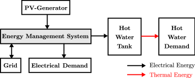
Figure 2: Energy flow in the smart home

II-A PV-Generator

The function that models the power output of the PV-generator dependant on the current irradiation and outside temperature is specified by

$$\begin{split}P^{PV}(t)=P_{PV,STC}\frac{I(t)}{I_{STC}}\Bigl{(}1-\gamma\Bigr{.}&\Bigl{.}\left(T_{j}(t)-T_{j,STC}\right)\Bigr{)}\\ &\cdot N_{PVs}N_{PVp}\ ,\end{split}$$ (1)

which is similar to the description in [7, 1]. In Eq. (1) the cell temperature $T_{j}(t)$ is modeled by

$$T_{j}(t)=T_{amb}(t)+\frac{I(t)}{I_{NOCT}}\left(NOCT-T_{amb,NOCT}\right)\ ,$$ (2)

where the variables and parameters $P_{PV}$, $P_{PV,STC}$, $I$, $I_{STC}$, $\gamma$, $T_{j,STC}$, $N_{PVs}$, $N_{PVp}$, $T_{amb}$, $NOCT$ in Eq. (1) and Eq. (2) describe the current total power output of all PV-modules, the power output of a PV-module under standard test conditions (STC), the current global irradiation on the sloped surface of the modules, the irradiation at STC, the power temperature coefficient at the maximum power point (MPP), the cell temperature at STC, the number of PV-modules in series, the number of PV-modules in parallel, the outside temperature, and the nominal operating cell temperature. According to [7] the parameters of the STC and NOCT measurement conditions are defined as $I_{STC}=1000W/m^{2}$, $T_{j,STC}=25^{\circ}C$, $I_{NOCT}=800W/m^{2}$, $T_{amb,NOCT}=20^{\circ}C$, at a wind speed of $1m/s$. The choices of other parameters will be given in the evaluation section. However, they are quite similar to the ones in [7].

II-B Hot Water Tank

In our simulation, we modified the hot water tank model, used in [9] and [10], in order to keep the complexity low. Specifically, a non-stratifying tank model is used, so that the water temperature can be assumed to be homogeneous. Furthermore, the volume of water in the tank is constant. This implies that the same amount of water, which is withdrawn from the tank is replaced with cold fresh water. In addition, the tank walls are not explicitly modeled. Instead they are implicitly considered with the constant $a$ which influences the speed of heat exchange with the surrounding air. Different from the models described in [9] and [10], we assume that the electrical heating element can take an arbitrary power value in the interval $[0,P_{max}]$. In other models, only discrete switching between maximum heating power and off is possible. Analyzing the thermal energy of the tank leads to the differential equation that models the behavior of the water temperature $T(t)$ in the tank as

$$\begin{split}\frac{d}{dt}T(t)=-\frac{a}{C}\left(T(t)-\right.&\left.T_{room}\right)-\frac{1}{m_{w}}W(t)\\ &\cdot\left(T_{out}-T_{in}\right)+\frac{P_{max}}{C}u(t)\ .\end{split}$$ (3)

with $C=c_{w}m_{w}$, the thermal capacity of the tank, $a$ a constant describing the heat transfer trough the tank walls, $c_{w}$ the specific thermal capacity of water, $m_{w}$ the mass of water in the tank, $W(t)$ the hot water abstraction for the desired temperature at time $t$, $T_{out}$ the desired hot water temperature, $T_{in}$ the cold water inlet temperature, and $P_{max}$ and $u(t)$ being the design heating power of the heating element in watts and the normed input to the heating element which can take values between $\left[0,1\right]$. It is worth mentioning that the specific thermal capacity of water is dependent on the water temperature. However, in this simulation, the specific thermal capacity of water is assumed to be constant to simplify calculations. This simplification introduces comparable small errors as the temperature at which the tank is operating only varies within a certain small interval.

III Smart Water Heater Control

The main goal of smart water heater control is to minimize the residents’ total electricity costs by optimizing the control of the temperature in the heated water tank. Additionally, the comfort of the residents’ should be maintained at all time. For this purpose, knowledge about the future hot water consumption, produced energy, electricity demand, and energy prices is required. As these quantities are unknown, an optimization algorithm has to rely on predictions of these values. Due to the uncertainty of predictions, it is necessary to model the unknown future consumption of hot water, produced power, electricity demand, and energy prices as random variables $\omega_{k}^{w}$, $\omega_{k}^{PV}$, $\omega_{k}^{el}$, and $\omega_{k}^{Pr}$, respectively, with $k$ being the current algorithm time step. In our setting, we assume that the prediction error is Gaussian distributed with zero mean and independent for each discrete simulation time step $k$. For example, the probability density function (PDF) for the random variable of the hot water consumption $f_{\omega_{k}^{w}}(\omega_{k}^{w})$ is $\mathcal{N}(\omega_{k}^{w,pred},{\sigma_{k}^{w}}^{2})$ distributed with $\omega_{k}^{w,pred}$ as outcome of the hot water consumption prediction. The standard deviation $\sigma_{k}^{w}$ is chosen according to the uncertainty of the particular prediction which is also assumed to be known. The PDFs of the other random variables are constructed in a similar way. Using these random variables and the dynamic of the hot water tank from Eq. (3), the DP algorithm seeks an optimal control for a finite horizon in order to minimize the energy costs.

Before the optimization algorithm can be applied, it is necessary to describe the problem in an appropriate mathematical form. First of all, the continuous time $t$ is discretized into equal time steps of length $\Delta t$ and a total simulation time length of $N$ steps. Furthermore, the tank temperature $T(k\cdot\Delta t)$ is also discretized and in the following represented by the discrete state $x_{k}$. The normed input of the hot water heater is also discrete and denoted by $u_{k}$. The system state transition function $f(x_{k},u_{k},\omega_{k})$, required by the DP algorithm, relates the next state $x_{k+1}$ with the current state $x_{k}$, input $u_{k}$, and disturbance $\omega_{k}$. Such a relationship is implicitly given by Eq. (3). However, an analytical solution of this differential equation is not available. Thus, Eq. (3) is integrated over the time step $\Delta t$ using a trapezoidal method and assuming that the hot water consumption and input are constant during that time step. Finally, the equation is solved for $x_{k+1}$, resulting in an approximation of the sought-after explicit relationship

$$\begin{split}x_{k+1}\!=&rd\Biggl{(}\!\!\left(1\!+\!\frac{a\Delta t}{2C}\right)^{\!-1}\!\!\left(\!\left(1-\frac{a\Delta t}{2C}\right)x_{k}\!+\!\frac{a}{C}T_{room}\Delta t\right.\Biggr{.}\\ &\biggl{.}\left.-\frac{1}{m_{w}}\omega_{k}^{w}\left(T_{out}-T_{in}\right)\Delta t+\frac{P_{max}}{C}u_{k}\Delta t\right)\Biggr{)}\ .\end{split}$$ (4)

The rounding operator $rd(\cdot)$ in Eq. (4) is needed due to the discrete modeling of the states $x_{k}$.

In the present case, the amount on the energy bill shall be reduced. Hence, an intuitive choice for the stage costs is the amount of money which is paid for the exchange of energy with the grid during a time step. The exchanged electricity with the grid is the difference between produced and consumed electrical energy in the smart home. Thus, the stage costs for one time step are

$$g_{k}(x_{k},u_{k},\omega_{k})=\left(\left(-\omega_{k}^{PV}+\omega_{k}^{el}+P_{max}u_{k}\right)\Delta t\right)\omega_{k}^{Pr}\,.$$ (5)

Using the definitions from above the mathematical optimization problem can be formulated.

Let us denote by $\Pi$ the space of all admissible policies. The DP algorithm now seeks an optimal policy $\pi^{*}=\{\mu_{0}^{*},\dots,\mu_{N-1}^{*}\}\in\Pi$ which minimizes, given a start state $x_{0}$, the cost-to-go function

$$\!J_{\pi^{*}}(x_{0})\!=\!\min_{\pi\in\Pi}\operatorname*{\mathbb{E}}_{\{\omega_{k}\}}\!\!\left\{g_{N}(x_{N})\!+\!\!\sum_{k=0}^{N-1}g_{k}(x_{k},\mu(x_{k}),\omega_{k})\right\}\,$$ (6)

for the considered horizon $N$. For this purpose, the optimal action $u_{k}^{*}=\mu_{k}^{*}(x_{k})$ for every state at each time step needs to be calculated. This is achieved by applying the DP algorithm which can be stated according to [6] in the following way: The algorithm starts from the terminal state $x_{N}$ by defining the costs of the final step as

$$J_{N}(x_{N})=g_{N}(x_{N})\ .$$ (7)

Afterwards, the algorithm recursively computes the cost-to-go of every state at each time step $k=N-1,N-2,\ldots,1,0$ using

$$\begin{split}J_{k}(x_{k})=\min_{u_{k}\in U_{k}(x_{k})}\operatorname*{\mathbb{E}}_{\{\omega_{k}\}}&\Big{\{}g_{k}(x_{k},u_{k},\omega_{k})\\ &+J_{k+1}\left(f(x_{k},u_{k},\omega_{k})\right)\Big{\}}.\end{split}$$ (8)

The control $u_{k}$ which minimizes the right side of Eq. (8) is the optimal control $u_{k}^{*}$ to apply when the system is in state $x_{k}$. Thus, minimizing the cost-to-go of each state for every time step $k$ will deliver the optimal policy $\pi^{*}$. In order to solve Eq. (8) it is necessary to calculate the included expected value considering the contained random variables $\omega_{k}^{w}$, $\omega_{k}^{PV}$, $\omega_{k}^{el}$, and $\omega_{k}^{Pr}$. For this purpose, we assume that the random variables are both independent of each other and independent among different time steps. Furthermore, we can split the expected value of Eq. (8) by applying the linearity of the expectation operator, i.e.

$$\begin{split}\operatorname*{\mathbb{E}}_{\{\omega_{k}\}}&\left\{g_{k}(x_{k},u_{k},\omega_{k})+J_{k+1}\left(f(x_{k},u_{k},\omega_{k})\right)\right\}=\\ &\operatorname*{\mathbb{E}}_{\{\omega_{k}\}}\!\!\left\{g_{k}(x_{k},u_{k},\omega_{k})\right\}+\!\!\!\!\operatorname*{\mathbb{E}}_{\{\omega_{k}\}}\left\{J_{k+1}\left(f(x_{k},u_{k},\omega_{k})\right)\right\}.\end{split}$$ (9)

As the stage costs defined in Eq. (5) is a linear combination and multiplication of random variables assumed to be independent, the following equality holds for the expected value of the stage costs

$$\begin{split}\operatorname*{\mathbb{E}}_{\{\omega_{k}\}}\!\!\left\{g_{k}(x_{k},u_{k},\omega_{k})\right\}=&\biggl{(}\!\Bigl{(}-\operatorname*{\mathbb{E}}_{\{\omega_{k}\}}\{\omega_{k}^{PV}\}+\operatorname*{\mathbb{E}}_{\{\omega_{k}\}}\{\omega_{k}^{el}\}\Bigr{.}\biggr{.}\\ &\biggl{.}\Bigl{.}+P_{max}u_{k}\Bigr{)}\Delta t\biggr{)}\operatorname*{\mathbb{E}}_{\{\omega_{k}\}}\{\omega_{k}^{Pr}\}\,.\end{split}$$ (10)

In the case of the second summand of Eq. (9), a similar approach is unfortunately not feasible due to the non-linearity of the rounding operator in $f(x_{k},u_{k},\omega_{k})$ and the cost-to-go function $J_{k+1}$. As a sequel, the expected value has to be determined in a different way as

$$\begin{split}\!\!\operatorname*{\mathbb{E}}_{\{\omega_{k}\}}\!\!\left\{J_{k+1}\left(f_{k}(x_{k},u_{k},\omega_{k})\right)\right\}\!=\!\!\int_{-\infty}^{\infty}&\!\!J_{k+1}\left(f(x_{k},u_{k},\omega_{k}^{w})\right)\\ &\cdot f_{\omega_{k}^{w}}(\omega_{k}^{w})\mathrm{d}\omega_{k}^{w}.\end{split}$$ (11)

However, it is not possible to simply integrate over this expression due to the discrete states $x_{k}$ and the rounding operator in $f(x_{k},u_{k},\omega_{k})$. Thus, our method determines first the likelihood that a certain state $x_{k+1}$ appears. For this purpose, the lower and upper bounds $(\omega_{k}^{w,low},\omega_{k}^{w,up})$ of the hot water consumption interval which leads according to Eq. (4) to state $x_{k+1}$ have to be determined. This is done using Eq. (4) without the rounding operator resulting in a modified function $f^{\prime}(x_{k},u_{k},\omega_{k}^{w})$. As the upper and lower bounds $(T_{k}^{up},T_{k}^{low})$ of the tank temperature interval, which is mapped on the discrete state $x_{k+1}$ by the rounding operator, are known, these boundaries can be plugged into the modified Eq. (4) which is solved for $\omega_{k}^{w,low}$ and $\omega_{k}^{w,up}$, respectively. Considering $x_{k}$ and $u_{k}$ as constants during one time step the calculation of the lower and upper limit of the hot water consumption interval which is mapped on the state $x_{k+1}$ can be stated as

$$\omega_{k}^{w,low} =f^{\prime-1}(x_{k},u_{k},T_{k}^{up})$$ (12)

$$\omega_{k}^{w,up} =f^{\prime-1}(x_{k},u_{k},T_{k}^{low})\ ,$$ (13)

with $f^{\prime-1}$ being the inverted function of $f^{\prime}$. Now, as the limits of the interval $\left[\omega_{k}^{w,low},\omega_{k}^{w,up}\right]$, which is mapped for a particular combination of $x_{k}$ and $u_{k}$ to a certain state $x_{k+1}$ are known, the probability that a state $x_{k+1}$ appears can be calculated as

$$\Pr(x_{k+1})=\int_{\omega_{k}^{w,low}}^{\omega_{k}^{w,up}}{f_{\omega_{k}^{w}}(\omega_{k}^{w})\mathrm{d}\omega_{k}^{w}}\ .$$ (14)

Using Eq. (14) it is feasible to rewrite Eq. (11) in a discretized form as

$$\operatorname*{\mathbb{E}}_{\{\omega_{k}\}}\!\!\left\{J_{k+1}\left(f_{k}(x_{k},u_{k},\omega_{k})\right)\right\}\approx\!\!\sum_{\forall x_{k+1}}\!\!{J_{k+1}\left(x_{k+1})\right)\Pr(x_{k+1})}.$$ (15)

As a result, the expected value in Eq. (8) can be computed, and consequently, a DP algorithm can be successfully applied to the Smart Home. Further details about the experimental setting of the Smart Home and the missing variable values are given in the next section.

IV Experimental setting

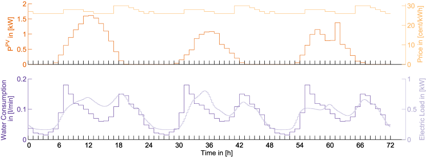
Figure 3: Predicted input data for three days.

In our experiment, we ran the simulation of the water tank along with our control algorithm over the course of several simulated days. For the sake of readability, in the figures only the results for a three day timespan are depicted and effects that only occur in the long run are described alongside if they are of relevance. We assume noisy prediction data to accommodate a broad range of forecasting algorithms. These predictions are generated by assuming consumption and production values for a typical household and are plotted in Fig. 3. The PV-generator output is directly derived using above model together with natural weather data of the city of Munich. The other values are derived from publicly available datasets. Afterwards additive Gaussian noise with a standard deviation of $\sigma_{k}^{w,gen}=\frac{2}{3}\omega_{k}^{w,pred}$, $\sigma_{k}^{PV,gen}=\frac{0.5}{3}\omega_{k}^{PV,pred}$, $\sigma_{k}^{el,gen}=\frac{1}{3}\omega_{k}^{el,pred}$ and $\sigma_{k}^{Pr,gen}=\frac{5}{3}\omega_{k}^{Pr,pred}$ for hot water consumption, PV-generator output, electrical power consumption and energy price is added to the input data for each experiment, respectively. Here, variables with a superscript of $gen$ indicate the standard deviations used in the experiment and variables with a superscript of $pred$ indicate that this value is taken from the input data at time step $k$. To compensate for eventual influences of our additive noise, each experiment is averaged over 20 independent runs.

To make the solution of the DP problem feasible, continuous time, control input to the water tank, and temperatures have to be discretized. As we chose a control time interval of 15 $min$, which is typical for a relatively inert system such as a water tank, the simulation over three days consists of $N=288$ total timesteps. The water tank temperature is discretized with an interval of $\Delta x=0.1^{\circ}C$ and the control input with $\Delta u=0.05$. A more limited classical setting where the heater can only be switched on or off, could be reproduced by discretizing the control input to two steps only.

In order to prevent the growth of harmful microorganisms, the temperature in the hot water circulation of a domestic house should always be above $60^{\circ}C$. Therefore, we set the interval for the ideal water tank temperature to be in $[T_{min}=60^{\circ}C,T_{max}=80^{\circ}C]$. However, these interval bounds are not strictly enforced in the experiment depicted in Fig. 4 and Fig. 5.

The remaining parameters of the model are summarized in Table I, where $N_{PV_{s}}$ denotes the number of solar panels in series and $N_{PV_{p}}$ the number of panels connected in parallel. All model parameters were designed to reflect an average household configuration and were selected in accordance with [9, 7].

TABLE I: Model Parameters

	Name	Value	Unit
PV-	$N_{PVs}$	5	-
Generator	$N_{PVp}$	2	-
	$NOCT$	45.5	${}^{\circ}C$
	$\gamma$	0.00043	$1/^{\circ}C$
	$P_{PV,STC}$	165	$W$
Hot	$a$	128.38	$J/min^{\circ}C$
Water	$c_{w}$	4.1813	$J/g^{\circ}C$
Tank	$m_{w}$	196.82	$kg$
	$C$	$8.22\cdot 10^{5}$	$J/^{\circ}C$
	$T_{in}$	10	${}^{\circ}C$
	$T_{out}$	60	${}^{\circ}C$
	$T_{room}$	22	${}^{\circ}C$
	$P_{max}$	4.5	$kW$

We compared our stochastic DP algorithm to two other state of the art Dynamic Programming algorithms. The first is a shortest path version of optimization for smart home control [7]. In this variant the discretized water heater temperature serves as state in a grid that is spanned on one axis by the time steps and on the other by the temperature values. The algorithm then aims to optimize total cost by searching backwards, finding the shortest path through this fully connected grid of states. The second DP algorithm variant we compared to, is a deterministic variant, cf. [11]. It is similar to our stochastic algorithm but without explicitly considering the effects of prediction and state transition uncertainties. Namely, this algorithm calculates the optimal solution assuming the real system behaves exactly like the model given the predicted input data without noise. This is a significant difference to our approach in that we can consider possible uncertainties about the prediction, in particular the hot water consumption, and take them into account for further upcoming action scheduling.

A simple Proportional Integral (PI) controller, which is most commonly found in classical water heaters with a variably controllable heating element, serves as baseline algorithm. We do not include other algorithms in the field of optimal heater control, as they either do not take the uncertainty of the consumption prediction into account, e.g. [12] or have to be pre-trained extensively involving a tedious parameter tuning, cf. [8].

V Results

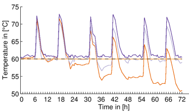
Figure 4: Simulated water tank temperature for three days (dynamic pricing).

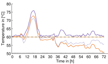
Figure 5: Simulated water tank temperature for three days (fixed price).

In Fig. 4 the water temperature for a three-day simulation is depicted using the dynamic pricing scheme. The setpoint of the hot water tank is $60^{\circ}C$ (horizontal dashed line) and it can be noticed that the temperature curve of the PI controller (yellow line) is constantly holding the desired tank temperature. On the other hand, other algorithms start pre-heating the tank in order to compensate for the upcoming hot water consumption.

All DP based method have similar pre-heating behaviour as they all access the same prediction values. Therefore, at the beginning the behaviour is very similar. As the predictions turn out to be unreliable, the algorithms that do not consider uncertainty start to decrease in their performance (shortest path in orange, deterministic DP in light purple). Violations of the lower temperature bound happen more and more often, while the stochastic DP algorithm (dark purple line) can cope with such unexpected fluctuations. This gap in behaviour amplifies if the runtime of the experiment is increased. Similar behaviour can be observed, when using a fixed pricing scheme, as can be seen in Fig. 5. our proposed Stochastic DP algorithm manages to maintain a temperature at or above the setpoint, while the other two DP algorithms struggle when unforeseen water consumption occurs.

In Table II, the sum of total violations of temperature bounds are summed up for the considered three day period. Clearly, the simple shortest path modelling turns out to be unstable to unforeseen fluctuations as well as deterministic DP. As a low water temperature can cause significant inconvenience for the house residents and can even make harmful microorganisms to grow, we implemented a compensation mechanism.

As soon as the temperature falls below $60^{\circ}C$, the next actions are not determined with the total costs as an optimization target, but to provide a correction. They are called corrective actions. Clearly, those actions increase the total amount of power used. This behaviour can also be observed in Fig. 6 for fixed energy prices. In this graph the total costs that accumulated are plotted. While for the unmodified algorithms, the two deterministic DP algorithms (solid lines) have the advantage of using less energy which has to be bought from the grid, at the same time they perform poorly with respect to temperature stability. If corrective actions are implemented, the total costs of the two deterministic algorithms are more or less the same (dotted lines) as in the stochastic DP case. It is to be noted that all three DP algorithms can achieve the goal of increasing eigen consumption through pre-heating at lower energy costs than the PI controller.

TABLE II: Total Costs and Violation of Temperature Bounds

Method	no corrective action		corrective actions
	Cost/€	# of violations	Cost/€	# of violations
PI-Control	9.0755	-	9.0755	-
shortest Path	8.0080	179	8.7484	21
deterministic DP	8.6612	123	8.7631	30
stochastic DP	8.7712	0	8.7712	0

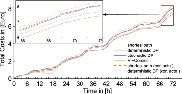
Figure 6: Accumulated costs graph for a fixed pricing scheme.

VI Conclusions

In this paper, we developed a stochastic DP algorithm for controlling water heater in the scenario of smart home. Our algorithm demonstrated its promising capability to ensure that the tank always contains a sufficient amount of hot water to satisfy the demand despite the uncertainty in the warm water consumption prediction. Furthermore, convincing results show the feasibility to reduce the energy costs at the same time. The reason for this is twofold. Firstly, the eigen consumption is increased, enabled by the use of a thermal storage instead of selling to the power grid. Secondly, the algorithm leverages forecasts of the PV-system output, water consumption, electrical demand, and energy prices.

References

- [1] D. Brunelli and L. Tamburini, “Residential load scheduling for energy cost minimization,” in Energy Conference (ENERGYCON), 2014 IEEE International, May 2014, pp. 675–682.
- [2] E. Galvan-Lopez, C. Harris, L. Trujillo, K. Rodriguez-Vazquez, S. Clarke, and V. Cahill, “Autonomous demand-side management system based on monte carlo tree search,” in Energy Conference (ENERGYCON), 2014 IEEE International, May 2014, pp. 1263–1270.
- [3] Q. Wei, D. Liu, G. Shi, Y. Liu, and Q. Guan, “Optimal self-learning battery control in smart residential grids by iterative q-learning algorithm,” in Adaptive Dynamic Programming and Reinforcement Learning, IEEE Symposium on, Dec 2014, pp. 1–7.
- [4] S. Squartini, D. Fuselli, M. Boaro, F. De Angelis, and F. Piazza, “Home energy resource scheduling algorithms and their dependency on the battery model,” in Computational Intelligence Applications In Smart Grid (CIASG), 2013 IEEE Symposium on, April 2013, pp. 122–129.
- [5] R. Welch and G. Venayagamoorthy, “Optimal control of a photovoltaic solar energy system with adaptive critics,” in Neural Networks, 2007. IJCNN 2007. International Joint Conference on, Aug 2007, pp. 985–990.
- [6] D. P. Bertsekas, Dynamic programming and optimal control. Athena Scientific Belmont, MA, 1995.
- [7] Y. Riffonneau, S. Bacha, F. Barruel, and S. Ploix, “Optimal power flow management for grid connected pv systems with batteries,” Sustainable Energy, IEEE Transactions on, vol. 2, no. 3, pp. 309–320, July 2011.
- [8] D. Fuselli, F. De Angelis, M. Boaro, D. Liu, Q. Wei, S. Squartini, and F. Piazza, “Optimal battery management with adhdp in smart home environments,” in Advances in Neural Networks. Springer Berlin Heidelberg, 2012, vol. 7368, pp. 355–364.
- [9] J.-C. Laurent, G. Desaulniers, R. Malhame, and F. Soumis, “A column generation method for optimal load management via control of electric water heaters,” Power Systems, IEEE Transactions on, vol. 10, no. 3, pp. 1389–1400, Aug 1995.
- [10] C. Chong and A. Debs, “Statistical synthesis of power system functional load models,” in Decision and Control including the Symposium on Adaptive Processes, 1979 18th IEEE Conference on, vol. 2, Dec 1979, pp. 264–269.
- [11] H. Tischer and G. Verbic, “Towards a smart home energy management system - a dynamic programming approach,” in Innovative Smart Grid Technologies Asia (ISGT), 2011 IEEE PES, Nov 2011, pp. 1–7.
- [12] P. Du and N. Lu, “Appliance commitment for household load scheduling,” Smart Grid, IEEE Transactions on, vol. 2, no. 2, pp. 411–419, June 2011.