COMPARISON OF CME/SHOCK PROPAGATION MODELS WITH HELIOSPHERIC IMAGING AND IN SITU OBSERVATIONS

Abstract

The prediction of the arrival time for fast coronal mass ejections (CMEs) and their associated shocks is highly desirable in space weather studies. In this paper, we use two shock propagation models, i.e. Data Guided Shock Time Of Arrival (DGSTOA) and Data Guided Shock Propagation Model (DGSPM), to predict the kinematical evolution of interplanetary shocks associated with fast CMEs. DGSTOA is based on the similarity theory of shock waves in the solar wind reference frame, and DGSPM on the non-similarity theory in the stationary reference frame. The inputs are the kinematics of the CME front at the maximum speed moment obtained from the geometric triangulation method applied to STEREO imaging observations together with the Harmonic Mean approximation. The outputs provide the subsequent propagation of the associated shock. We apply these models to the CMEs on 2012 January 19, January 23, and March 7. We find that the shock models predict reasonably well the shock's propagation after the impulsive acceleration. The shock's arrival time and local propagation speed at Earth predicted by these models are consistent with in situ measurements of WIND. We also employ the Drag-Based Model (DBM) as a comparison, and find that it predicts a steeper deceleration than the shock models after the rapid deceleration phase. The predictions of DBM at 1 AU agree with the following ICME or sheath structure, not the preceding shock. These results demonstrate the applicability of the shock models used here for future arrival time prediction of interplanetary shocks associated with fast CMEs.

1 Introduction

Coronal mass ejections (CMEs) are large-scale eruptions of plasma and magnetic field from the Sun into interplanetary (IP) space. Soon after their discovery in the 1970s, CMEs were regarded as major sources for severe space weather events (Sheeley et al., 1985; Gosling, 1993; Dryer, 1994). For example, the geoeffective CME would be a threat for astronauts performing space activity, spacecraft, navigation & communication systems, airplane-passengers at high altitudes, ground power grids & pipelines (e.g., Boteler et al. (1998); Lanzerotti (2005); National Research Council (2008)). Fast CMEs often lead to strong IP shocks ahead of them when propagating in the heliosphere, and the shocks have additional space weather effects, such as producing solar energetic particle (SEP) events (Gopalswamy et al., 2003; Cliver & Ling, 2009), compressing the geo-magnetosphere when colliding with the Earth (Green & Baker, 2015), and even causing a ``tsunami'' throughout the whole heliosphere (Intriligator et al., 2015). Therefore, predicting arrival times of these fast CMEs/shocks at the Earth has become a significant ingredient of space weather forecasting. Various kinds of models in this aspect have been developed during the past decades, such as empirical models, physics-based models, and MHD models. Zhao & Dryer (2014) gave an overall review for these models as well as their current applications.

The models in arrival time prediction usually adopt the observables of CMEs/shocks obtained near the Sun as inputs to predict whether/when they will arrive at the Earth. The in situ observations at L1 spacecraft are then used to verify the prediction results. In other words, the predictions are carried out only at two ends, i.e. inputs on the Sun and outputs near the Earth. A prediction for the CME/shock's propagation could not be checked by observations beyond 30 solar radii ($R_{s}$) in the heliosphere during the SOHO era because the field of view (FOV) of SOHO/LASCO is within this distance. The launch of STEREO in 2006 heralded a new epoch for studies in this area. In contrast to SOHO, the FOV of the imaging telescopes (HI1/HI2) onboard STEREO allows CMEs/shocks to be tracked over much longer distances, even beyond the Earth's orbit. Techniques have been developed to track solar disturbances based on the wide-angle imaging observations of STEREO, e.g., the triangulation technique developed by Liu et al. (2010a) has no free parameters and can determine the CME/shock kinematics as a function of distance. This triangulation technique initially assumes a relatively compact CME structure simultaneously seen by the two STEREO spacecraft. Lugaz et al. (2010) and Liu et al. (2010b) later incorporate into the triangulation concept to a spherical front attached to the Sun for the geometry of wide CMEs (see detailed discussions on the CME geometry assumptions in the triangulation technique by Liu et al. (2010b, 2016)). The triangulation technique with these two CME geometries has been successfully applied to investigate the propagation of CMEs through and their interactions with the inner heliosphere between the Sun and Earth (e.g., Liu et al. (2010a, b, 2013, 2016); Lugaz et al. (2010); Davies et al. (2013); Mishra & Srivastava (2013)).

In this paper, we present our improved shock propagation models that utilize the early kinematics of the CME front as input, and predict the shock's propagation in the subsequent IP space and its arrival time at a given distance from the Sun. In particular, these predictions will be verified not only by the in situ measurements at 1 AU but also by direct imaging of STEREO in IP space. This study attempts to make qualitative comparisons between model predictions and wide-angle imaging observations over long distances in the heliosphere. The investigation will improve our understanding of the kinematics of the CMEs/shocks during their outward propagation in IP space.

2 THEORETICAL MODELS

2.1 Data Guided Shock Time Of Arrival

In the similarity theory of shocks, the similarity variable $\eta=r/R(t)$ was adopted, where $r$ is distance and $R(t)$ is the shock position at time $t$. Then a similarity solution was sought in which the velocity, density, and pressure were rewritten as functions of the non-dimensional similarity variable (Rogers, 1958; Sedov, 1959; Parker, 1961; Dryer, 1974). Such a solution maintains its similarity form. According to the similarity solution, the shock's kinematics can be described in terms of normalized ambient conditions, and are governed by its expansion effect. The shock front keeps its shape when propagating outward. Once a shock is identified in terms of a general limiting condition, then one may note that it ``remembered'' its genesis (Dryer, 1974). In this solution, the propagation speed ($V_{b}$) of a spherically symmetric blast wave (no further energy ejected) in an ambient medium with density decreasing in square of radial distance is (Parker, 1961; Dryer, 1974):

$$V_{b}\sim R^{-0.5}$$ (1)

Here $V_{b}$ is in the reference frame of the ambient medium, $R$ is the radial distance from the wave source. For the case of IP shock, its propagation speed ($V_{s}$) in the stationary frame is computed as $V_{s}=V_{b}+V_{SW}$; $V_{SW}$ is the ambient solar wind speed. As one of the physics-based models in the shock arrival time prediction, the ``Shock Time Of Arrival'' (STOA) model assumes that the shock is initially driven by an ejecta at a constant speed. After this initial driven phase, the shock front propagates outward as a blast wave at the $R^{-0.5}$ deceleration speed (Dryer, 1974; Dryer & Smart, 1984; Smart & Shea, 1984, 1985). The initial shock velocity is derived from the observed Type II radio burst drifting speed, and the driving time duration is estimated from the X-ray flux of the associated flare. Direct observations of STEREO/SECCHI can provide the kinematics of the CME front over long distances in the heliosphere, therefore we use direct observations to replace the constant-speed assumption made in STOA, named a Data Guided Shock Time Of Arrival (DGSTOA). In DGSTOA, the $R^{-0.5}$ speed dependence relation is assumed to be valid for the CME-associated shock after the CME completes its impulsive acceleration and reaches the maximum speed near the Sun. Impulsive accelerations of fast CMEs are found to be common (Zhang et al., 2001; Cheng et al., 2010; Zhao et al., 2010; Liu et al., 2011, 2013). Assuming that the shock has propagated to distance $R_{M}$ when the front of the associated CME reaches its maximum speed $V_{M}$, then the shock's propagation speed $V_{s}$ (in the stationary reference frame) at any subsequent distance $R$ can be computed as:

$$V_{s}=\frac{dR}{dt}=\left(V_{M}-V_{SW}\right)\left(\frac{R}{R_{M}}\right)^{-0.5}+V_{SW}$$ (2)

The numerical integral of $\frac{1}{V_{s}}$ provides the shock's transit time $TT(R)$ from $R_{M}$ to $R$:

$$TT(R)={\int_{R_{M}}}^{R}\frac{1}{V_{s}(R^{\prime})}dR^{\prime}$$ (3)

In order to predict whether the shock can persist to the Earth, we follow the judge index adopted in the STOA model. The ambient solar wind and interplanetary magnetic field (IMF) parameters observed by L1 spacecraft at the start time of the event are used to compute the sound speed $C_{S}$ and Alfvén speed $V_{A}$. Then the shock's magnetoacoustic Mach number $M_{a}$ is derived as a measure of the shock strength:

$$M_{a}=\frac{V_{SE}-V_{SW}}{\sqrt{{C_{S}}^{2}+{V_{A}}^{2}}}$$ (4)

Here $V_{SE}$ is the shock's local speed at Earth computed from Equation (2) (in the stationary reference frame). The background solar wind speed $V_{SW}$ is taken from the in situ measurements of L1 spacecraft at the start time of the event. If $M_{a}>1$, the shock is predicted to reach the Earth; otherwise, it is predicted to decay to become MHD waves before reaching the Earth.

2.2 Data Guided Shock Propagation Model

Different from the similarity theory, Wei (1982) and Wei & Dryer (1991) studied in the stationary reference frame the propagation of blast waves from a point source in a moving, steady-state, medium with variable density. They considered both the expansion effects of the shock and the convection effects of the background flow. In their non-similarity solution, the shape and kinematics of the shock are determined by the balance between the initial blast energy and the background flow. They obtained the following analytical solution to describe the propagation of the blast wave:

$$V_{s}=\frac{dR}{dt}=\left[-2\lambda_{1}+\sqrt{(2\lambda_{1})^{2}+\frac{E_{0}}{J_{0}R}+\frac{1}{2J_{0}}}\right]V_{SW}$$ (5)

Here, $V_{s}$ is shock speed in the stationary reference frame at distance $R$, $t$ is time, $V_{SW}$ is solar wind speed (taken from L1 spacecraft at the start time), and $E_{0}$ is the dimensionless form of the initial total energy ($E_{s}$) that the blast released into the background medium, i.e., $E_{0}=\frac{E_{s}}{AV_{SW}^{2}}$ where $A$ = 300 kg m^-1. $J_{0}=\frac{3}{8}$ and $\lambda_{1}=-0.1808$ are constants of the coefficients of the solution. However, the energy released by a blast cannot be observed directly. Feng & Zhao (2006) and Zhao & Feng (2014) combined the empirical method of estimating the shock's initial energy used in the ISPM model (Smith & Dryer, 1990, 1995), i.e. $E_{s}=C.V_{si}^{3}.\omega.(\tau+D)$, with this non-similarity solution of blast waves and proposed the ``Shock Propagation Model'' (SPM) (Feng & Zhao, 2006) and its second version (SPM2) (Zhao & Feng, 2014). Here $V_{si}$ is the shock initial speed computed from Type II drifting speed. $\tau$ is the piston-driving time duration estimated from the X-ray flux of the associated flare. $\omega$ denotes the solid angular width of the shock and is assumed to be $60^{\circ}$ because it could not be determined accurately. $C$ (=0.283$\times 10^{20}$ erg.m^-3.sec^-2.deg^-1) and $D$ (=0.52 hr) are two constants. Zhao & Feng (2015) continued to incorporate the kinematical parameters (velocity, angular width) of CMEs observed by SOHO/LASCO with characteristics of the accompanied solar flare-Type II events into the initial energy estimation of the associated shock, and put forward a third version of the model (SPM3). In SPM3, the prediction success rate on whether the shock would arrive at Earth had been improved greatly. However, the improvement in the arrival time prediction remained limited. The reasons for this poor improvement mainly came from two aspects. On one hand, the CME velocity used in Zhao & Feng (2015) is the projected speed on the plane of sky (POS) of SOHO, which does not represent the propagation speed of the CME along the Sun-Earth direction. On the other hand, the blast wave theory does not apply to the initial acceleration phase of the CME/shock because there is no additional energy added to the system in the blast wave theory. The impulsive acceleration phase demonstrates that continuous energy is still energy fed into the CME/shock system which leads to the impulsive acceleration. Therefore, we decided to present a Data Guided Shock Propagation Model (DGSPM) that uses the tracking results of STEREO for fast CMEs during their initial acceleration phases as inputs to predict the propagation and arrival time of their associated shocks in the following deceleration phases.

Let us assume that the eruption occurs at $t=0$. The CME front reaches its maximum speed $V_{M}$ when $t=t_{M}$ at the radial distance $R_{M}$. The DGSPM model assumes that the blast wave theory starts to be valid for the CME-associated shock at $R_{M}$. According to Equation (5):

$$V_{M}=\left[-2\lambda_{1}+\sqrt{(2\lambda_{1})^{2}+\frac{E_{0}}{J_{0}R_{M}}+\frac{1}{2J_{0}}}\right]V_{SW}$$ (6)

Therefore,

$$E_{0}=J_{0}R_{M}\left[\left(2\lambda_{1}+\frac{V_{M}}{V_{SW}}\right)^{2}-(2\lambda_{1})^{2}-\frac{1}{2J_{0}}\right]$$ (7)

From this equation we can estimate the initial energy of a shock given $V_{M}$ and $R_{M}$ of the associated CME front. Then, the integral of $\frac{1}{V_{s}}$ from Equation (5) gives the transit time $TT(R)$ of the shock to any subsequent distance $R$:

$$TT(R)=\frac{J_{0}}{V_{SW}}\left\{4\lambda_{1}\left[R+2E_{0}-2E_{0}ln(R+2E_{0})\right]+2\sqrt{\frac{E_{0}}{J_{0}}R+\left(4\lambda_{1}^{2}+\frac{1}{2J_{0}}\right)R^{2}}-\frac{\left(16\lambda_{1}^{2}+\frac{1}{J_{0}}\right)E_{0}}{\sqrt{4\lambda_{1}^{2}+\frac{1}{2J_{0}}}}\right.$$

$$\times ln\left[\sqrt{\frac{E_{0}}{J_{0}}R+\left(4\lambda_{1}^{2}+\frac{1}{2J_{0}}\right)R^{2}}+(R+2E_{0})\sqrt{4\lambda_{1}^{2}+\frac{1}{2J_{0}}}-\frac{\left(16\lambda_{1}^{2}+\frac{1}{J_{0}}\right)E_{0}}{2\sqrt{4\lambda_{1}^{2}+\frac{1}{2J_{0}}}}\right]$$

$$\left.-8\lambda_{1}E_{0}ln\left[\frac{\sqrt{\frac{E_{0}}{J_{0}}R+\left(4\lambda_{1}^{2}+\frac{1}{2J_{0}}\right)R^{2}}+4\lambda_{1}E_{0}}{R+2E_{0}}-\frac{16\lambda_{1}^{2}+\frac{1}{J_{0}}}{8\lambda_{1}}\right]\right\}+TT_{0}~{}~{}~{}~{}~{}~{}~{}~{}~{}~{}~{}~{}$$ (8)

Here, $TT_{0}$ is determined by the restriction of $R=R_{M}$ when $TT=t_{M}$. Accordingly, the propagation speed of the shock at distance $R$ is again computed from Equation (5).

In order to predict whether or not the shock will persist to the Earth, an index suggested by Zhao & Feng (2015) is adopted in the DGSPM. The Equivalent Shock Strength Index (ESSI) is defined as:

$$ESSI=\frac{V_{s}(EL)-V_{SW}}{V_{F}}$$ (9)

Here, $V_{s}(EL)$ is the local speed of shock at Earth, $V_{F}$ is the fast-mode wave speed of the background solar wind at Earth, given by $V_{F}^{2}=0.5[V_{A}^{2}+C_{S}^{2}+\sqrt{(V_{A}^{2}+C_{S}^{2})^{2}-4V_{A}^{2}C_{S}^{2}cos^{2}\theta}]$. $\theta$ is the angle between the shock normal and the local magnetic field. In this study, we use the ambient solar wind and IMF conditions in situ observed by the L1 spacecraft at the start time of the event to compute $V_{A}$, $C_{S}$, and $V_{F}$ ($\theta$ assumed to be 45^∘ or 135^∘). A threshold value (ESSI_tv) needs to be set to predict whether the shock could persist to the Earth. Zhao & Feng (2015) tested 498 events of Solar Cycle 23 and found that ESSI combined with the CME angular width ($AW_{CME}$) could give the maximum successful predictions. Here, $AW_{CME}$ is the angular width of the CME projected onto the POS of SOHO. Zhao & Feng (2015) set the threshold values as ESSI${}_{tv}=1.53$ and $AW_{tv}=121^{\circ}$ by fitting all the 498 events. As a study for case events, we do not need to set new threshold values. We just follow the criteria established in Zhao & Feng (2015), i.e.: if ESSI $\geqslant$ ESSI${}_{tv}=1.53$ and $AW_{CME}\geqslant AW_{tv}=121^{\circ}$, then the shock is predicted to be able to persist to the Earth, and its transit time is predicted based on Equation (2.2); Otherwise, the shock is predicted to miss the Earth.

3 APPLICATION TO THREE EVENTS

Based on the wide-angle imaging observations of COR2, HI1, and HI2 onboard two STEREO spacecraft, Liu et al. (2013) studied the whole Sun-to-Earth propagation of three CME events during 2012, which are 2012 January 19 (Case 1), 2012 January 23 (Case 2), and 2012 March 7 CMEs (Case 3). They are fast CMEs with maximum initial speeds of 1300–2300 km/s. These fast CMEs are not very common during the long-lasting low solar active period, and are interesting subjects to the space weather community. The tracking for these CME fronts was implemented by a combination of the geometric triangulation technique developed by Liu et al. (2010a, b) and the Harmonic Mean (HM) approximation developed by Lugaz et al. (2009, 2010) (this combination is called the HM triangulation for abbreviation in the following). The triangulation results in the near Sun regions obtained by Liu et al. (2013) will be adopted in this study as inputs of prediction models. The corresponding prediction results are also compared with the tracked kinematics of the CME front in the subsequent Sun-to-Earth journey.

3.1 2012 January 19 Event

3.1.1 Model Input

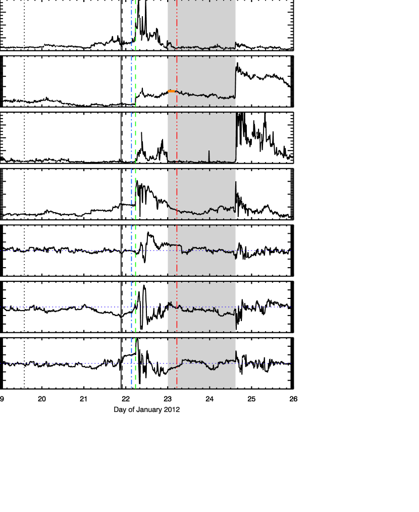
Figure 2: The in situ observations of the WIND spacecraft from 2012 January 19 to 2012 January 25. The panels display the proton density (n_p), bulk speed (v_p), proton temperature (T_p), total magnetic field ($\mid$ B $\mid$) and its three components (B_x, B_y, B_z) in the GSE coordinate system from top to bottom. The vertical dotted line denotes the CME launch time, the vertical green dashed line denotes the shock, and the shaded region denotes the ICME interval. The times of the shock arrival and ICME interval are taken from Liu et al. (2013). The arrival times predicted by DGSPM, DGSTOA, HM, and DBM are indicated by the vertical solid line, dashed line, blue dashed-dotted line, and red dashed-dotted line, respectively. The horizontal pink line in the bulk speed plot represents the average speed across the ICME leading boundary.

The inputs of DGSTOA and DGSPM for this event are as follows. The CME was launched at 13:55:00 UT on 2012 January 19, and it was accelerated to max speed $V_{M}$=1362 km/s at the radial distance $R_{M}$=15.67 $R_{s}$ at 18:45:54 UT ($t_{M}$) (Liu et al., 2013), which is taken to be the start time of model predictions. The projected angular width of this CME ($AW_{CME}$) is $360^{\circ}$ in the POS of SOHO/LASCO. The solar wind speed ($V_{SW}$) at 1 AU is about 350 km/s observed by the WIND spacecraft at the CME launch time, and the following ambient solar wind and IMF parameters at 1 AU are used to compute $C_{S}$, $V_{A}$, and $V_{F}$: proton density $n$ = 5.8 cm^-3, proton temperature $T_{p}=0.7\times 10^{5}$ K, IMF magnetude $B$ = 4.3 nT (see Figure 2). The parameters $V_{M}$, $R_{M}$, $t_{M}$, $V_{SW}$, $C_{S}$, $V_{A}$, $V_{F}$ are input into Equations (2)–(4) for DGSTOA and Equations (5)–(9) for DGSPM. The angular width $AW_{CME}$ is also required by DGSPM in order to predict whether or not the shock will persist to the Earth.

In addition to DGSTOA and DGSPM, we also use the Drag-Based Model (DBM) (Vrs̆nak et al., 2013) to give predictions as a comparison. This model assumes that beyond a certain distance the dynamics of CMEs are governed solely by the interaction between interplanetary CME (ICME) and the ambient solar wind, and the drag acceleration has a quadratic dependence on their relative speed. This DBM model has four free parameters, i.e. ``take-off speed'' $v_{0}$, starting radial distance $r_{0}$, ambient solar wind speed $w$, and drag coefficient $\gamma$. Here, we take $v_{0}$=$V_{M}$, $r_{0}$=$R_{M}$, $w$=$V_{SW}$. We fit the distance-time plot predicted by the DBM with different $\gamma$ to that of the HM triangulations from $R_{M}$ to $R_{M}$+50 $R_{s}$ (see Figure 1) to give the best drag coefficient, which is $\gamma=9.8\times 10^{-8}$ km^-1 for this event. Then the DBM with this finally determined value of $\gamma$ is adopted to predict the propagation of the CME front beyond $R_{M}$+50 $R_{s}$.

3.1.2 Observation and Prediction from the Sun to Earth

Figure 1 shows a comparison between the observations of STEREO for the CME front (HM triangulation) and predictions of the models (DGSPM, DGSTOA, DBM) for the distance-time plot (top) and velocity-distance plot (bottom). In this figure, the blue solid circles are the tracked results of the HM triangulation for the CME front. We can see that this CME underwent an initial impulsive acceleration, and it reached the max speed 1362 km/s ($V_{M}$) at the end of this acceleration phase at $R$ =15.67 $R_{s}$ ($R_{M}$); then, the CME experienced a rapid deceleration from 15.67 $R_{s}$ to about 50 $R_{s}$; finally, it propagated outward with a gradual deceleration (Liu et al., 2013). The application of the triangulation technique requires that the CME front is observed by two STEREO spacecraft simultaneously. For this case, the CME front was tracked by the triangulation method continuously out to about 160 $R_{s}$, and a linear extrapolation to 1 AU gave the predicted arrival time of the shock at 03:11:00 UT on January 22 (Liu et al., 2013). Similarly, the shock's propagation speed at the Earth predicted by the HM triangulation was obtained by computing the average velocity during the time when the CME front keeps nearly a constant speed. This yielded 665 km/s for the shock speed (Liu et al., 2013). DGSPM and DGSTOA are applicable beyond $R_{M}$. The DGSPM prediction is denoted by the solid line, DGSTOA prediction denoted by the dashed line, and DBM prediction denoted by the red dashed-dotted line. The predictions of the two shock models (DGSPM, DGSTOA) are similar, and differences between them are very small for this case. They both roughly agree with the HM triangulation. Specifically speaking, DGSPM predicts that the shock would have reached Earth at 21:14:04 UT on 2012 January 21, and the shock's propagation speed at the Earth would be 653 km/s. DGSTOA predicts that the shock would have encountered Earth at 21:53:12 UT on 2012 January 21 with the local propagation speed of 623 km/s. According to DBM, the arrival time and local speed at 1 AU would be 05:10:02 UT on 2012 January 23 and 383 km/s, respectively.

The in situ measurements of WIND at 1 AU demonstrated that the corresponding shock arrived at Earth at 05:32:58 UT on January 22 (Liu et al., 2013), and the shock's local propagation speed along the Sun-Earth direction was 466 km/s (see section 3.1.3) as shown by green stars in Figure 1. Therefore, the prediction errors of DGSPM for the shock's arrival time and local propagation speed at Earth are 8.31 hours (hr) and -187 km/s, respectively. Similarly, corresponding errors of DGSTOA are 7.66 hr and -157 km/s. As a comparison, prediction errors of the HM triangulation are 2.37 hr and -199 km/s. On the other hand, the kinematics of the CME front beyond 40 $R_{s}$ predicted by DBM are evidently slower than the HM triangulation. As a result, the DBM prediction fits the propagation of the following ICME instead of the preceding shock. The arrival time and local propagation speed of ICME at WIND are shown as green triangles in Figure 1. The ICME speed (455 km/s) at 1 AU is defined as the average speed across the ICME leading boundary (see section 3.1.3). The prediction errors of DBM for ICME arrival time and local speed are -5.17 hr and 72 km/s, respectively.

In contrast with the HM triangulation, both shock models (DGSPM, DGSTOA) did not reproduce the rapid deceleration phase of the CME front between $R_{M}$ and 50 $R_{s}$. Two reasons may be responsible for this deficiency. On one hand, the shock models adopted here are single-fluid models, which ignore the energy loss due to accelerating local particles at the shock front. The energy of the energetic particles can be a large portion of the total kinetic energy of the CME (Mewaldt et al., 2008). As envisioned by Liu et al. (2013, 2016), the energy loss to energetic particles through shock acceleration may partly account for the rapid deceleration. On the other hand, the solar wind speed is assumed to be a constant from the Sun to Earth in these models, which is taken from the in situ measurements of WIND at 1 AU. In fact, the background solar wind should undergo a steady acceleration through most of the distance within 30 $R_{s}$ (Sheeley et al., 1997), and the corresponding solar wind speeds in these regions are definitely slower than the 1 AU speed. The overestimating of the ambient solar wind speed in these regions increased the convection effect of the background flow, and weakened the shock's rapid deceleration as a result. As to DBM, the input parameter $\gamma$ was determined by fitting the predicted distance-time plot to that of the HM triangulations in the range from $R_{M}$ to $R_{M}$+50 $R_{s}$. Therefore, this model successfully reproduced the rapid deceleration of the CME front during this stage. However, DBM continued to predict a fast deceleration of the CME front at large distances, and its prediction lagged both the predictions of the shock models and the HM triangulation results for the CME's leading edge more and more. As a result, the arrival time predicted by DBM agreed better with that of the ICME, rather than with that of the preceding shock. The propagation speed at 1 AU predicted by DBM also agreed reasonably well with the average speed across the ICME leading boundary.

3.1.3 Comparison with In Situ Measurements

Figure 2 displays the in situ observations of the WIND spacecraft from 2012 January 19 to January 25. From top to bottom, the panels in this figure display the proton density (n_p), bulk speed (v_p), proton temperature (T_p), total magnetic field ($\mid$ B $\mid$) and its three components (B_x, B_y, B_z) in the Geocentric Solar Ecliptic (GSE) coordinate system. The vertical dotted line denotes the CME launch time. The green dashed line indicates the shock front. The arrival times predicted by DGSPM, and DGSTOA are represented as the black solid line and black dashed line, respectively. The blue dashed-dotted line is the arrival time predicted by the HM triangulation. The shaded region is the ICME structure following the shock (Liu et al., 2013). We define the ICME local speed as the averaged flow speed across the ICME leading boundary, which is 455 km/s for this event (see the pink line in the bulk speed plot). The red dashed-dotted line represents the arrival time predicted by DBM. This figure shows that the arrival times predicted by DGSPM, DGSTOA, and HM triangulation are close to the shock arrival time detected by WIND. But all predictions are earlier than the real arrival time. The arrival time predicted by DBM is late and falls inside the ICME interval, but close to the ICME leading boundary.

The local propagation speed of the shock can be computed from the upstream and downstream solar wind parameters:

$$\textbf{V}_{sh}=\frac{\rho_{2}\textbf{v}_{2}-\rho_{1}\textbf{v}_{1}}{\rho_{2}-\rho_{1}}$$ (10)

Here $\rho_{1}$, $\rho_{2}$ are the average density in the upstream and downstream regions; $\textbf{v}_{1}$, $\textbf{v}_{2}$ are the corresponding average velocity; $\textbf{V}_{sh}$ is the velocity vector of the shock front. As predictions of all these methods (HM triangulation, DGSPM, DGSTOA) are made along the Sun-Earth line, we compute the shock's propagation speed in the Sun-Earth direction, i.e. $V_{sh}=\textbf{V}_{sh}\textbf{.}\textbf{n}_{SE}$. Here $\textbf{n}_{SE}$ is the unit vector of the Sun-Earth direction.

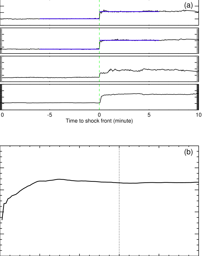
Figure 3: The upstream and downstream solar wind parameters (n_p, v_p, T_p, $\mid$ B $\mid$) of 3-second resolution for the shock at 05:32:58 UT on 2012 January 22 (a) and the shock propagation speed ($V_{sh}$) plotted against the averaging window size in the upstream and downstream regions. In (a), the blue solid lines indicate the averages of solar wind density and velocity in the upstream and downstream regions. In (b), the vertical dotted line corresponds to 6 minutes of the averaging window size finally selected.

As an example, Figure 3 demonstrates how we compute the shock's local speed at 1 AU. We use the high-resolution (3 second) data of the WIND observation to compute the upstream and downstream solar wind parameters. Figure 3(a) displays solar wind parameters (n_p, v_p, T_p, $\mid$ B $\mid$) in the upstream and downstream regions of the shock at 05:32:58 UT on 2012 January 22. Here, time is indicated relative to the shock front (green dashed line). Negative time corresponds to the upstream region, and positive time to the downstream region. The shock jump is very sharp in this case. The solar wind parameters vary smoothly both upstream and downstream. Figure 3(b) shows the computed shock speed $V_{sh}$ for different averaging windows on either side of the shock front. We find that the computed $V_{sh}$ increases gradually with growing size of the averaging window from 0 to 3 minutes, then $V_{sh}$ decreases slightly from 3 to 6 minutes. After 6 minutes, $V_{sh}$ nearly stays constant at 466 km/s. There is no generally valid standard to define the averaging window size. We take the saturation level, here 466 km/s, as the in situ observed shock speed. The blue solid lines in Figure 3(a) indicate the averages of solar wind parameters $\rho_{1}$, $\rho_{2}$, $v_{1}$, $v_{2}$ in the upstream and downstream regions with 6 minutes of averaging interval. The local speed of the shock estimated above is slightly higher than the averaged flow speed (415 km/s) in the sheath region between the shock and ICME, but is closer to the predicted values of models (665 km/s of HM triangulation, 653 km/s of DGSPM, 623 km/s of DGSTOA). For clarity, Table 1 lists the input & output parameters of the models (HM, DGSPM, DGSTOA, DBM) and the in situ observations for this case.

For a brief summary to this case, predictions of the two shock models (DGSPM, DGSTOA) did not reproduce the rapid deceleration phase of the CME front. But they ``kept up'' with the shock in the following journey, and predicted both the arrival time and propagation speed of the shock at Earth reasonably well. Although DBM successfully reproduced the rapid deceleration of the CME, it lagged the shock front more and more in the subsequent propagation. As a result, the prediction of DBM pointed to the ICME behind the shock. The inputs of DGSPM and DGSTOA are the kinematical parameters of the CME front when it was accelerated to maximum speed, while the free input parameter $\gamma$ of DBM needs to be determined by fitting to the propagation process of the CME front during its deceleration phase. Therefore, the prediction results of DGSPM and DGSTOA were obtained earlier than those of DBM. All inputs of these models were obtained from the HM triangulation results based on STEREO observations.

3.2 2012 January 23 Event

3.2.1 Model Input

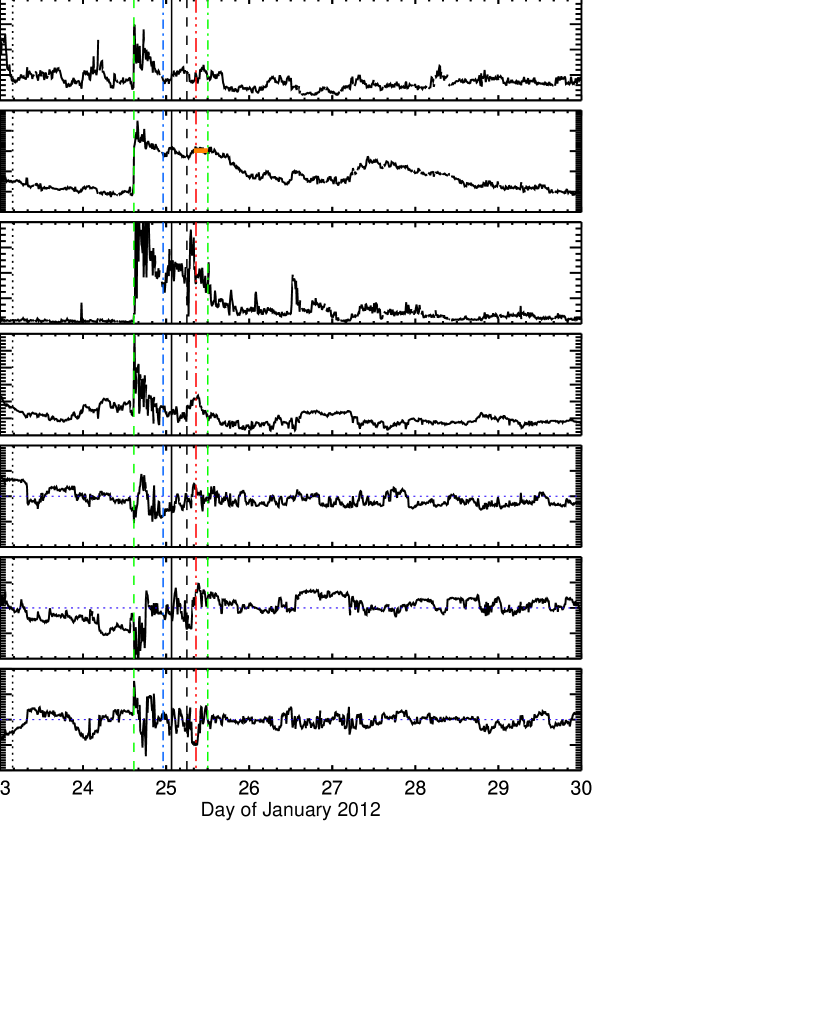
Figure 5: Similar to Figure 2, but for the in situ observations of WIND from 2012 January 23 to January 29, including the 1 AU observations for the 2012 January 23 CME event. No ICME signatures are observed at WIND except the shock (Liu et al., 2013), and the shock arrival time is taken from Liu et al. (2013). The green dashed-dotted line denotes the back boundary of the sheath structure. The pink line in the bulk speed plot represents the average flow speed across the sheath's tail part.

The inputs of DGSTOA and DGSPM for this event are as follows. The CME was launched at 03:40 UT on 2012 January 23, and it was accelerated to max speed $V_{M}$=1542 km/s at the radial distance $R_{M}$=12.24 $R_{s}$ at 05:35:54 UT ($t_{M}$) (Liu et al., 2013), which is the start time of the model predictions. $AW_{CME}$ is $360^{\circ}$ in the POS of SOHO/LASCO. $V_{SW}$ at 1 AU is about 460 km/s detected by the WIND spacecraft at the CME launch time, and the following ambient solar wind and IMF parameters at 1 AU are used to compute $C_{S}$, $V_{A}$, and $V_{F}$: $n$ = 10.0 cm^-3, $T_{p}=0.3\times 10^{5}$ K, $B$ = 11.1 nT (see Figure 5). The parameters $V_{M}$, $R_{M}$, $t_{M}$, $V_{SW}$, $C_{S}$, $V_{A}$, $V_{F}$ are input into Equations (2)–(4) for DGSTOA and Equations (5)–(9) for DGSPM. $AW_{CME}$ is also adopted by DGSPM to predict whether or not the shock will persist to the Earth. We take $v_{0}$=$V_{M}$, $r_{0}$=$R_{M}$, $w$=$V_{SW}$ for the DBM model, and derive the drag coefficient $\gamma=3.4\times 10^{-8}$ km^-1 by fitting the model predictions to STEREO observations for the CME front (HM triangulation results) in the distance range from $R_{M}$ to $R_{M}$+50 $R_{s}$. Then, the DBM with this finally determined value of $\gamma$ is adopted to predict the propagation of the CME beyond $R_{M}$+50 $R_{s}$.

3.2.2 Observation and Prediction from the Sun to Earth

Figure 4 demonstrates a comparison between the observation of STEREO and the predictions of the models (DGSPM, DGSTOA, DBM) for the distance-time plot (top) and velocity-distance plot (bottom) of the CME front. Definitions of lines and symbols in this figure are the same as those in Figure 1. After the impulsive acceleration, this CME underwent a clear deceleration phase from $R_{M}$ to about 70 $R_{s}$. But this deceleration is not as strong as for the 2012 January 19 CME event shown in Figure 1. For example, the propagation speed of the CME decreased from 1542 km/s only to 900 km/s when distance increased from $R_{M}$ to 90 $R_{s}$. The shock models (DGSPM, DGSTOA) match reasonably well the HM triangulation results during this deceleration stage. Beyond 70 $R_{s}$, the HM triangulation yields a nearly constant-speed propagation of the CME front, and the shock models predict a gradual deceleration. The prediction of DGSPM is more consistent with the HM triangulation than DGSTOA during this phase. DBM predicts a weaker deceleration within 70 $R_{s}$ than DGSPM and DGSTOA, but a stronger deceleration beyond 70 $R_{s}$. For this case, the HM triangulation tracked the CME front continuously out from the Sun to beyond the Earth orbit, and it predicted that the shock would have reached Earth at 23:06:00 UT on 2012 January 24 with the local propagation speed of 900 km/s at 1 AU (Liu et al., 2013). DGSPM predicts that the shock would have arrived at Earth at 01:13:15 UT on 2012 January 25 with the local propagation speed of 799 km/s. DGSTOA predicts that the shock would have encountered Earth at 03:40:06 UT on 2012 January 25 with the local speed of 718 km/s. DBM predicts that the ICME would have reached Earth at 06:59:48 UT on 2012 January 25 with the local speed of 604 km/s at 1 AU.

The in situ measurements of WIND at 1 AU demonstrated that the corresponding shock arrived at Earth at 14:40:06 UT on January 24 (Liu et al., 2013), and the shock's local propagation speed along the Sun-Earth direction was 719 km/s (see section 3.2.3), shown as green stars in Figure 4. The shock arrived earlier than all predictions. The best prediction for the arrival time comes from the HM triangulation with the error of -8.43 hr. The prediction errors of the shock arrival time are -10.55 hr and -13.0 hr for DGSPM and DGSTOA, respectively. The fast propagation of the shock for this case might be due to its interaction with an earlier event as pointed out by Liu et al. (2013). Although models predict delayed arrival times, the shock's local propagation speeds at Earth predicted by them are very close to the speed computed from the in situ observations. The predictions errors are -181 km/s for HM, -80 km/s for DGSPM, and 1 km/s for DGSTOA. No ICME structure was found in the WIND observations for this shock event (Liu et al., 2013). But we can see a clear sheath region downstream the shock with high fluctuations in solar wind parameters. The sheath structure ended at about 12:00 UT of January 25, and the average speed across its back boundary was around 602 km/s. If we relate the prediction of DBM to the sheath's back boundary (SBB), then the prediction errors for arrival time and 1 AU local speed are only 5.0 hr and -2 km/s.

3.2.3 Comparison with In Situ Measurements

Figure 5 displays the in situ observations of the WIND spacecraft from 2012 January 23 to January 29. Definition of each line in this figure is the same as in Figure 2. The green dashed-dotted line denotes the back boundary of the sheath structure. The pink line in the bulk speed plot represents the averaged flow speed across the sheath's tail part. The shock arrival time (green dashed line) is earlier than prediction of any model. We need to point out that this shock had propagated into the ICME structure associated with the January 19 CME event, and the interaction should have occurred inside 1 AU. This shock formed the back boundary of the preceding ICME. The former ICME offered a low density and strong magnetic field background medium for the propagation of this shock. Both low density and strong magnetic field increased the Alfvén speed of the ambient medium, which would cause a faster advance of the shock than predicted. A similar analysis can be found in Liu et al. (2013). The arrival time of the ICME predicted by DBM is 5 hours earlier than the ending time of the sheath structure. In the same way as for the 2012 January 19 event, we compute the in situ speed of the shock along the Sun-Earth line based on the WIND observations, which is 719 km/s. Similarly, this local speed of the shock is slightly higher than the averaged flow speed (650 km/s) in the sheath region, and is closer to the predicted values of models (900 km/s of HM triangulation, 799 km/s of DGSPM, 718 km/s of DGSTOA) as well. The detailed input & output parameters of the models (HM, DGSPM, DGSTOA, DBM) as well as the in situ observations for this case are also listed in Table 1.

As a brief summary, this CME decelerated more slowly during the rapid deceleration phase than the 2012 January 19 CME. Shock models (DGSPM, DGSTOA) successfully reproduced this deceleration process for this case. However, the shock propagated faster at larger distances than all model predictions possibly due to the interaction with the earlier ICME. As a result, the actual shock arrival time was earlier than those predicted by DGSPM and DGSTOA. But the shock's local propagation speed at 1 AU computed from the upstream and downstream solar wind parameters matched predictions of the models reasonably well, and this local speed of the shock was faster than the sheath region flow speed. The corresponding ICME associated with this shock was not recorded by WIND at 1 AU. The prediction of DBM pointed to the back boundary of the sheath structure.

3.3 2012 March 7 Event

3.3.1 Model Input

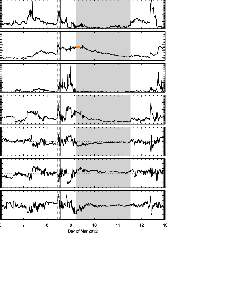
Figure 7: Similar to Figure 2, but for the in situ observations of WIND from 2012 March 6 to March 12, including the 1 AU observations for the 2012 March 7 CME event. The times of the shock arrival and ICME interval are taken from Liu et al. (2013). The pink line in the bulk speed plot represents the average speed across the ICME leading boundary.

This CME was launched at 00:15 UT on 2012 March 7, and it was accelerated to max speed $V_{M}$=2369 km/s at the radial distance $R_{M}$=15.20 $R_{s}$ at 02:36:36 UT ($t_{M}$) (Liu et al., 2013). This time is taken to be the start time of shock models. $AW_{CME}$ is $360^{\circ}$ in the POS of SOHO/LASCO, $V_{SW}$ at 1 AU is about 375 km/s detected by the WIND spacecraft at the CME launch time, and the following ambient solar wind and IMF parameters at 1 AU are used to compute $C_{S}$, $V_{A}$, and $V_{F}$: $n$ = 5.8 cm^-3, $T_{p}=0.3\times 10^{5}$ K, $B$ = 8.3 nT (see Figure 7). The parameters $V_{M}$, $R_{M}$, $t_{M}$, $V_{SW}$, $V_{A}$, $C_{S}$, $V_{F}$ are input into Equations (2)–(4) for DGSTOA and Equations (5)–(9) for DGSPM. $AW_{CME}$ is also required by DGSPM in order to predict whether or not the shock will persist to the Earth. We take $v_{0}$=$V_{M}$, $r_{0}$=$R_{M}$, $w$=$V_{SW}$ for DBM, and derive the drag coefficient $\gamma=6.2\times 10^{-8}$ km^-1 by fitting the model predictions to STEREO observations for the CME front (HM triangulations) in the distance range from $R_{M}$ to $R_{M}$+50 $R_{s}$. Finally, the DBM with this finally determined value of $\gamma$ is used to predict the propagation of the CME beyond $R_{M}$+50 $R_{s}$.

3.3.2 Observation and Prediction from the Sun to Earth

Figure 6 shows observations of STEREO and predictions of the models (DGSPM, DGSTOA, DBM) for the distance-time plot (top) and velocity-distance plot (bottom) of the CME front. Definitions of lines and symbols in this figure are the same as those in Figure 1. Similar to the 2012 January 19 CME event, this CME underwent a rapid deceleration from $R_{M}$ to about 50 $R_{s}$. The deceleration occurred over a distance of only 35 $R_{s}$, but the velocity decreased from 2369 km/s to about 1000 km/s. Again, the shock models (DGSPM, DGSTOA) could not reproduce this rapid deceleration, but the shock velocity evolution predicted by them are consistent with the HM triangulation results during the gradual deceleration phase beyond 100 $R_{s}$. The DBM successfully reproduced the rapid deceleration from $R_{M}$ to 50 $R_{s}$. But it gave a too slow propagation beyond 60 $R_{s}$. For this case, the CME front was tracked by the HM triangulation continuously out only to 150 $R_{s}$; the arrival time of the shock and its propagation speed at 1 AU predicted by HM could be determined by linear extrapolations, which gave 17:55:00 UT on 2012 March 8 and 950 km/s, respectively (Liu et al., 2013). DGSPM predicts that the shock would have arrived at Earth at 13:34:18 UT on 2012 March 8 with the local propagation speed of 873 km/s. DGSTOA predicts that the shock would encountered Earth at 12:12:36 UT on 2012 March 8 with the local speed of 905 km/s. DBM predicts that the ICME would have reached Earth at 17:24:36 UT on 2012 March 9 with the local speed of 444 km/s.

The in situ measurements of WIND at 1 AU demonstrated that the corresponding shock encountered Earth at 10:30:45 UT on March 8 (Liu et al., 2013), and the local propagation speed of the shock along the Sun-Earth direction was 1088 km/s (see section 3.3.3), shown as green stars in Figure 6. The arrival times predicted by the shock models (DGSPM, DGSTOA) are very close to the observed one, and their prediction errors are only -3.06 hr for DGSPM and -1.70 hr for DGSTOA. The corresponding errors in the local shock speed are 215 km/s (DGSPM) and 183 km/s (DGSTOA), respectively. Predictions of the HM triangulation are worse for the arrival time with an error of -7.40 hr but better for the shock speed with an error of 138 km/s. The associated ICME arrived at 1 AU at 05:00 UT on March 9 and lasted until 12:20 UT on March 11 (Liu et al., 2013). The averaged flow speed across the ICME leading boundary was 717 km/s (see section 3.3.3). The predictions of DBM are 12.41 hr late for the arrival time and fall short by 273 km/s for the ICME speed at 1 AU.

3.3.3 Comparison with In Situ Measurements

Figure 7 shows the in situ observations of the WIND spacecraft from 2012 March 6 to March 12. Definition of each line in this figure is the same as that in Figure 2. The shock arrival time (green dashed line) is earlier than the predictions of the models (HM, DGSPM, DGSTOA). But the differences between them are small. The shaded region is the interval of the following ICME structure (Liu et al., 2013), which has a low density and temperature, decreasing velocity, enhanced magnetic field strength, and a smooth rotation of the magnetic field direction. The arrival time predicted by DBM lies within the ICME interval, 12.41 hr later than the arrival of the ICME leading boundary. In the same way, we compute the in situ speed (1088 km/s) of the shock along the Sun-Earth direction based on the WIND observations. Similarly, this shock speed is faster than the averaged flow speed (680 km/s) observed in the sheath region, and is closer to the predicted values of models (950 km/s of HM triangulation, 873 km/s of DGSPM, 905 km/s of DGSTOA). Table 1 summarizes the input & output parameters of the models (HM, DGSPM, DGSTOA, DBM) and the in situ observations for this case.

For a summary, the rapid deceleration of this CME front from $R_{M}$ to 50 $R_{s}$ was successfully reproduced by DBM, but not by the shock models (DGSPM, DGSTOA). The velocity evolutions predicted by DGSPM and DGSTOA matched the HM triangulation results in the subsequent gradual deceleration phase, and they gave reasonably good predictions not only for the shock arrival time but also for the shock's local speed at Earth. The predictions of DBM corresponded to the ICME structure following the shock, but the predicted arrival time lagged the ICME leading boundary by 12.41 hr. The shock speed computed from the upstream and downstream solar wind parameters described better the local propagation speed of the shock at 1 AU than the flow speed in the sheath region. The speeds predicted by the shock models were more consistent with the shock speed thus derived.

4 SUMMARY AND DISCUSSION

In this study we employed two models to predict the propagation of shocks associated with fast CMEs in the heliosphere, i.e. DGSTOA and DGSPM. The former is based on the similarity theory of blast waves in the ambient flow (solar wind) reference frame, and the latter on the non-similarity theory of blast waves in the stationary reference frame. The inputs of these models are kinematical characteristics of the associated CME front when the CME reaches its maximum speed close to the Sun, and these parameters are obtained from a continuous tracking for the white-light feature of a CME viewed in coordinated imaging of STEREO by the HM triangulation (Liu et al., 2013). We applied these models to three cases of the 2012 January 19 (Case 1), January 23 (Case 2), and March 7 (Case 3) CMEs/shocks, and found that the models can give a reasonable prediction for the propagation of the shock associated with fast CMEs after the initial impulsive acceleration phase. The shock's arrival time and local speed at Earth predicted by the models match generally well the in situ observations of WIND. We also used DBM to predict the arrival time and local speed at Earth, and found that its predictions agree better with the following ICME (Case 1 and Case 3) or sheath structure (Case 2) rather than with the preceding shock.

Table 2 summarizes the mean of the absolute prediction errors for the CME/shock arrival times and their local propagation speeds at Earth predicted by the HM triangulation, DGSPM, DGSTOA, and DBM. We can see that the mean of prediction errors for arrival times ranges from 6.0 to 7.6 hr, and the mean error for propagation speeds ranges from 110 to 180 km/s. The prediction accuracies of different models are similar. These predictions are reasonably good as far as we know. For example, Zhao & Dryer (2014) presented a review of current status of the prediction models for the CME/shock arrival time, and found that their prediction errors are about 10-12 hr at present. The prediction accuracies of arrival time derived in this study are improved by about 4-5 hr compared with them. Prediction results of DGSPM and DGSTOA are obtained earlier than those of DBM due to no free input parameter in the formers. The HM triangulation technique can provide a description about the whole propagation process of the CME front, including the impulsive acceleration, rapid deceleration, and slow deceleration phases (Liu et al., 2013). However, we need to point out that the shock models (DGSPM, DGSTOA) provided by this study may not apply to slow CMEs with initial speeds lower than the ambient solar wind speed. This kind of CMEs usually undergoes a gradual acceleration in the beginning, and then propagates outward at nearly a constant speed (Liu et al., 2016).

One reason for the prediction errors of the shock models may come from the uncertainties in the input parameters. For example, the maximum speed $V_{M}$ of the CME front is one of the most important input parameters. This parameter has uncertainties shown as blue error bars in Figure 1, Figure 4, and Figure 6. Specific speaking, the relative uncertainties of $V_{M}$ are 22.4% (305/1362) for Case 1, 11.8% (182/1542) for Case 2, and 14.0% (331/2369) for Case 3, respectively. As a comparison, the relative errors of the shock arrival time predicted by DGSPM are 13.1% (8.31/63.63), 30.1% (10.55/35.0), 8.9% (3.06/34.26), and those of the local shock speed at 1 AU are 40.1% (187/466), 11.1% (80/719), 19.8% (215/1088). The solar wind speed, adopted from 1 AU observations at the CME launch time, also does not represent the real flow speed just upstream of the shock. Considering so many input uncertainties, the prediction errors are acceptable. The shock speed computed from the upstream and downstream solar wind parameters is more consistent with the values predicted by the shock models than the average speed in the sheath.

The propagation processes of all three cases consist of three phases from the Sun to Earth: an initial impulsive acceleration, a rapid deceleration, and finally a gradual deceleration (Liu et al., 2013). The impulsive acceleration is caused by the Lorentz force, and ends up at a distance of 10-20 $R_{s}$. Predictions of DGSPM and DGSTOA start when the CME front reaches its maximum speed. But prediction of DBM starts at 50 $R_{s}$ (set empirically) further out because the drag coefficient ($\gamma$) needs to be determined by fitting. The rapid deceleration occurs over a very short distance from 10-20 $R_{s}$ to about 50 $R_{s}$. The shock models adopted here can not reproduce this rapid deceleration (for Case 1 and Case 3, Case 2 is better). An overestimation of the solar wind speed (taken from 1 AU), and therefore a too large convection of the ambient flow adopted in these models, can be one potential reason. Besides this, the energy loss due to accelerating the local energetic particles by the shock can be another reason (Liu et al., 2013), as this energy loss is not taken into account of in these single-fluid shock models. For example, Mewaldt et al. (2008) estimated that the total content of energy for energetic particles produced by shock can account for 10% of the associated CME's kinetic energy, or even more. As a contrast, DBM successfully reproduces this rapid deceleration as we fit the DBM predictions to the HM triangulation results in these regions to determine its free drag coefficient. The rapid deceleration evolves to a gradual deceleration at a distance around 50 $R_{s}$. Predictions of DGSPM and DGSTOA agree with the kinematics of the CME front tracked by the HM triangulation in this phase. The predicted shock arrival time and local propagation speed at Earth are consistent with the in situ measurements of WIND. However, the DBM predicts a stronger deceleration than the HM triangulation during this gradual deceleration stage, which indicates that a different $\gamma$ value may be needed for the gradual deceleration. This result implies that different physical mechanisms are responsible for the different deceleration processes, which cannot be described by a single drag-based deceleration process. The DBM predicted result lags the shock propagation more and more (see Figure 1, Figure 4, and Figure 6). At 1 AU, it's prediction agrees with the leading boundary of the ICME (Case 1 and Case 3) or the back boundary of the sheath (Case 2) behind the shock for both the arrival time and the local propagation speed. This may indicate that the standoff distance between the ICME and its preceding shock is increasing during their outward propagation.

It will lead to another point to be clarified: what is the nature of the CME front in the wide-angle imaging observations? As pointed out by Liu et al. (2011, 2013), the density within the CME is stronger than that of the preceding shock and sheath close to the Sun, therefore the white-light feature in imaging observations in these regions represents the front boundary of the CME main body; far away from the Sun, the density compression of the shock eventually dominates over that at the CME main body due to fast expansion of the CME, and the white-light feature gradually shifts to the preceding shock structure as a result. More direct evidences on this point will be investigated in future studies.

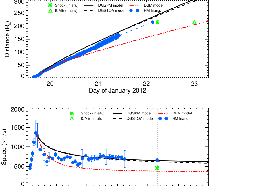
Figure 1: Comparison between imaging observations of STEREO and model predictions for the distance-time plot (up) and velocity-distance plot (bottom) for the 2012 January 19 event. The blue solid circles with error bars represent the HM triangulation results based on imaging observations of STEREO (Liu et al., 2013). The black solid and dashed lines denote the predictions of DGSPM and DGSTOA, respectively. The red dashed-dotted line denotes the prediction of DBM. The green star and triangle stand for the in situ measurements of WIND at 1 AU for the shock and ICME. The dotted lines denote the Earth location.

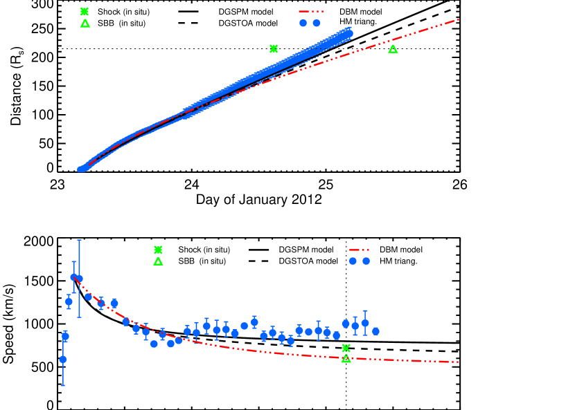
Figure 4: Similar to Figure 1, but for the 2012 January 23 CME event. SBB stands for the sheath's back boundary.

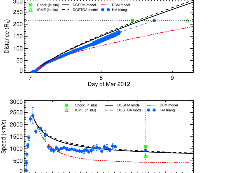
Figure 6: Similar to Figure 1, but for the 2012 March 7 CME event.

Table 1: The inputs & outputs of models, and in situ observations for these three cases.

		Case 1	Case 2	Case 3
CME launch time		2012.1.19 13:55:00 UT	2012.1.23 03:40:00 UT	2012.3.7 00:15:00 UT
Inputs	$t_{M}$	2012.1.19 18:45:54 UT	2012.1.23 05:35:54 UT	2012.3.7 02:36:36 UT
	$R_{M}$	15.67 $R_{s}$	12.24 $R_{s}$	15.20 $R_{s}$
	$V_{M}$	1362 km/s	1542 km/s	2369 km/s
	$AW_{CME}$	$360^{\circ}$	$360^{\circ}$	$360^{\circ}$
	$V_{SW}$	350 km/s	460 km/s	375 km/s
	$V_{A}$	39 km/s	77 km/s	75 km/s
	$C_{S}$	35 km/s	23 km/s	23 km/s
	$V_{F}$	49 km/s	79 km/s	77 km/s
	$\gamma$	$9.8\times 10^{-8}$ km-1	$3.4\times 10^{-8}$ km-1	$6.2\times 10^{-8}$ km-1
In situ	$t_{sh}$	2012.1.22 05:32:58 UT	2012.1.24 14:40:06 UT	2012.3.8 10:30:45 UT
observations	$V_{sh}$	466 km/s	719 km/s	1088 km/s
at	$t_{ICME}$	2012.1.23 00:00:00 UT	2012.1.25 12:00:00 UT	2012.3.9 05:00:00 UT
WIND	$V_{ICME}$	455 km/s	602 km/s	717 km/s
Outputs	$t_{sh,HM}$	2012.1.22 03:11:00 UT	2012.1.24 23:06:00 UT	2012.3.8 17:55:00 UT
	$V_{sh,HM}$	665 km/s	900 km/s	950 km/s
	$\Delta TT_{sh,HM}$	2.37 hr	-8.43 hr	-7.40 hr
	$\Delta V_{sh,HM}$	-199 km/s	-181 km/s	138 km/s
	$t_{sh,DGSPM}$	2012.1.21 21:14:04 UT	2012.1.25 01:13:15 UT	2012.3.8 13:34:18 UT
	$V_{sh,DGSPM}$	653 km/s	799 km/s	873 km/s
	$\Delta TT_{sh,DGSPM}$	8.31 hr	-10.55 hr	-3.06 hr
	$\Delta V_{sh,DGSPM}$	-187 km/s	-80 km/s	215 km/s
	$t_{sh,DGSTOA}$	2012.1.21 21:53:12 UT	2012.1.25 03:40:06 UT	2012.3.8 12:12:36 UT
	$V_{sh,DGSTOA}$	623 km/s	718 km/s	905 km/s
	$\Delta TT_{sh,DGSTOA}$	7.66 hr	-13.0 hr	-1.70 hr
	$\Delta V_{sh,DGSTOA}$	-157 km/s	1 km/s	183 km/s
	$t_{ICME,DBM}$	2012.1.23 05:10:02 UT	2012.1.25 06:59:48 UT	2012.3.9 17:24:36 UT
	$V_{ICME,DBM}$	383 km/s	604 km/s	444 km/s
	$\Delta TT_{ICME,DBM}$	-5.17 hr	5.0 hr	-12.41 hr
	$\Delta V_{ICME,DBM}$	72 km/s	-2 km/s	273 km/s

Note. $t_{M}$, and $R_{M}$ are the time and distance when CME front reaches the maximum speed ($V_{M}$). $AW_{CME}$ is the CME

angular width observed by SOHO/LASCO. $V_{SW}$ is the solar wind speed. $V_{A}$, $C_{S}$, and $V_{F}$ stand for the Alfvén speed,

sound speed, and fast-mode wave speed, respectively. $\gamma$ is the drag coefficient adopted by DBM. $t_{sh}$ and $V_{sh}$ are the

shock arrival time and local speed at WIND. $t_{ICME}$ and $V_{ICME}$ denote the arrival time and local speed of the ICME at

WIND; they correspond to the sheath's back boundary for Case 2. $t_{sh,HM}$ and $V_{sh,HM}$ represent the shock arrival time and

propagation speed at Earth predicted by HM; $\Delta TT_{sh,HM}$ and $\Delta V_{sh,HM}$ are their errors. Similarly, $t_{sh,DGSPM}$, $V_{sh,DGSPM}$,

$\Delta TT_{sh,DGSPM}$,$\Delta V_{sh,DGSPM}$ represent the prediction results and errors of DGSPM for the shock; $t_{sh,DGSTOA}$, $V_{sh,DGSTOA}$,

$\Delta TT_{sh,DGSTOA}$, $\Delta V_{sh,DGSTOA}$ represent those of DGSTOA for the shock; $t_{sh,DBM}$, $V_{sh,DBM}$, $\Delta TT_{sh,DBM}$, $\Delta V_{sh,DBM}$ represent

those of DBM for the ICME. Arrival times of the shock and ICME at WIND and the HM triangulation results are taken from

(Liu et al., 2013).

Table 2: The mean-absolute prediction errors for the CME/shock arrival times and their local propagation speeds at Earth predicted by the HM triangulation, DGSPM, DGSTOA, and DBM.

Prediction	Error of Arrival	Error of local
Method	Time (hr)	speed (km/s)
HM triang.	6.07	173
DGSPM	7.31	161
DGSTOA	7.45	114
DBM	7.53	116

References

- Boteler et al. (1998) Boteler, D. H., Pirjola, R. J., & Nevanlinna, H. 1998, Adv. Space Res., 22, 17
- Cheng et al. (2010) Cheng, X., Zhang, J., Ding, M. D., & Poomvises, W. 2010, ApJ, 712, 752
- Cliver & Ling (2009) Cliver, E. W., & Ling, A. G. 2009, ApJ, 690, 598
- Davies et al. (2013) Davies, J. A., Perry, C. H., Trines, R. M. G. M., et al. 2013, ApJ, 777, 167
- Dryer (1974) Dryer, M. 1974, Space Science Review, 15, 403
- Dryer (1994) Dryer, M. 1994, Space Sci. Rev., 67, 363
- Dryer & Smart (1984) Dryer, M., & Smart, D. F. 1984, Adv. Space Res., 4, 291
- Feng & Zhao (2006) Feng, X. S., & Zhao, X. H. 2006, Sol. Phys., 238, 167
- Gopalswamy et al. (2003) Gopalswamy, N., Yashiro, S., Lara, A., Kaiser, M. L., Thompson, B. J., Gallagher, P. T., & Howard, R. A. 2003, Geophys. Res. Lett., 30, 8015
- Gosling (1993) Gosling, J. T. 1993, J. Geophys. Res., 98(A11), 18937
- Green & Baker (2015) Green, L., & Baker, D. 2015, Weather, 70, 31
- Intriligator et al. (2015) Intriligator, D. S., Sun, W., Dryer, M., Intriligator, J., Deehr, C., Detman, T., & Webber, W. R. 2015, J. Geophys. Res., 120, 8267
- Lanzerotti (2005) Lanzerotti, L. J. 2005, Space Weather, 3, S05002
- Liu et al. (2010a) Liu, Y., Davies, J. A., Luhmann, J. G., et al. 2010a, ApJL, 710, L82
- Liu et al. (2010b) Liu, Y., Thernisien, A., Luhmann, J. G., et al. 2010b, ApJ, 722, 1762
- Liu et al. (2011) Liu, Y., Luhmann, J. G., Bale, S. D., & Lin, R. P. 2011, ApJ, 734, 84
- Liu et al. (2013) Liu, Y. D., Luhmann, J. G., Lugaz, N., Möstl, C., Davies, J. A., Bale, S. D., & Lin, R. P. 2013, ApJ, 769, 45
- Liu et al. (2016) Liu, Y. D., Hu, H., Wang, C., et al. 2016, ApJS, 222, 23
- Lugaz et al. (2009) Lugaz, N., Vourlidas, A., & Roussev, I. I. 2009, AnGeo, 27, 3479
- Lugaz et al. (2010) Lugaz, N., Hernandez-Charpak, J. N., Roussev, I. I., et al. 2010, ApJ, 715, 493
- Mewaldt et al. (2008) Mewaldt, R. A., Cohen, C. M. S., Giacalone, J., et al. 2008, in AIP Conf. Proc. 1039, Particle Acceleration and Transport in the Heliosphere and Beyond, ed. G. Li, Q. Hu, O. Verkhoglyadova et al. (Melville, NY: AIP), 111
- Mishra & Srivastava (2013) Mishra, W., & Srivastava, N. 2013, ApJ, 772, 70
- National Research Council (2008) National Research Council. 2008, Severe Space Weather Events–Understanding Societal and Economic Impacts: A Workshop Report (The National Academies Press).
- Parker (1961) Parker, E. N. 1961, ApJ, 133, 1014
- Rogers (1958) Rogers, M. H. 1958, Quart. J. Mech. Appl. Math., 9, 411
- Sedov (1959) Sedov L. I. 1959, Gostekhizdat, Moscow, 4th edition, 1957. English transl.: (M. Holt, ed.), Academic Press, New York.
- Sheeley et al. (1985) Sheeley Jr., N. R., Howard, R. A., Koomen, M. J., Michels, D. J., Schwenn, R., Mühlhäuser, K. H., & Rosenbauer, H. 1985, J. Geophys. Res., 90(A1), 163
- Sheeley et al. (1997) Sheeley Jr., N. R., Wang, Y.-M., Hawley, S. H., et al. 1997, ApJ, 484, 472
- Smart & Shea (1984) Smart, D. F., & Shea, M. A. 1984, in Proc. STIP Workshop on solar/interplanetary intervals, edited by M. A. Shea, D. F. Smart, and S. McKenna-Lawlor, p.139–256, Publ. Book Crafters, Chelsea, Michigan.
- Smart & Shea (1985) Smart, D. F., & Shea, M. A. 1985, J. Geophys. Res., 90, 183
- Smith & Dryer (1990) Smith, Z., & Dryer, M. 1990, Sol. Phys., 129, 387
- Smith & Dryer (1995) Smith, Z., & Dryer, M. 1995, NOAA Tech. Memo. ERL SEL-89, 123, 453
- Vrs̆nak et al. (2013) Vrs̆nak, B. et al., 2013, Sol. Phys., 285, 295
- Wei (1982) Wei, F. S. 1982, Chinese J. Space Sci., 2(1), 63
- Wei & Dryer (1991) Wei, F. S., & Dryer, M. 1991, Sol. Phys., 132, 373
- Zhang et al. (2001) Zhang, J., Dere, K. P., Howard, R. A., Kundu, M. R., & White, S. M. 2001, ApJ, 559, 452
- Zhao & Dryer (2014) Zhao, X. H., & Dryer, M. 2014,Space Weather, 12, 448
- Zhao et al. (2010) Zhao, X. H., Feng, X. S., Xiang, C. Q., et al. 2010, ApJ, 714, 1133
- Zhao & Feng (2014) Zhao, X. H., & Feng, X. S. 2014, J. Geophys. Res., 119, 1
- Zhao & Feng (2015) Zhao, X. H., & Feng, X. S. 2015, ApJ, 809, 44