Density and metallicity of the Milky-Way circumgalactic gas

Abstract

The halo of the Milky-Way circumgalactic gas extends up to the virial radius of the Galaxy, $\sim 250$ kpc. The halo properties may be deduced from X-ray spectroscopic observations and from studies of the ram-pressure stripping of satellite dwarf galaxies. The former method is more precise but its results depend crucially on the assumed metallicity of the circumgalactic gas; the latter one does not need these assumptions. Here, the information from both approaches is combined to constrain observationally the gas metallicity and density as functions of the galactocentric distance. It is demonstrated that the two kinds of data could be reconciled if the metallicity decreased to $Z\sim 0.1Z_{\odot}$ in the outer parts of the extended halo. The corresponding gas density profile is rather flat, falling as $r^{-(0.45\dots 0.75)}$ at large galactocentric distances $r$.

1 Introduction

Recently, considerable attention has been attracted to studies of gas coronae of galaxies, that is of reservoirs of gas extending up to the galaxies’ virial radii. This circumgalactic gas represents, thanks to the large volume it fills, a substantial contribution to the mass budget of a galaxy. This gaseous corona, or extended halo, of the Milky Way has attracted particular interest because of the “missing-baryon” problem, see e.g. Anderson & Bregman (2010), the apparent lack of baryons in our Galaxy compared to the amount expected, on average, from cosmology. On the other hand, interactions of cosmic rays with this circumgalactic gas have been considered as a possible source of important contributions to the diffuse gamma-ray (Feldmann, Hooper & Gnedin, 2013) and neutrino (Taylor, Gabici & Aharonian, 2014) backgrounds.

In the Milky Way, this reservoir of gas reveals itself in observations in two ways. First, the ram pressure of the gas strips dwarf satellite galaxies, whose orbits lay within the corona, from their own gas (Blitz & Robishaw, 2000). Second, the presence of the hot gas may be seen in X-ray spectra, either as zero-redshift absorption lines for extragalactic sources, or as emission lines in the blank-sky spectrum, see e.g. Gupta et al. (2012); Miller & Bregman (2013, 2015). Taken at face value, the gas density profiles derived by these two methods are inconsistent with each other. However, the spectroscopic approach is based on observations of spectral lines of oxygen, which is only a tracer of the full amount of gas. As a result, the gas density obtained by the spectroscopic method is very sensitive to unknown chemical composition of the gas, usually encoded in its metallicity $Z$. The aim of this work is to depart from simplified ad hoc assumptions about the metallicity of the Galactic corona and to use spectroscopic and ram-pressure results jointly, which allows us to constrain values and profiles of density and metallicity of the circumgalactic gas simultaneously, so that the agreement between all data is maintained.

The rest of the paper is organized as follows. In Sec. 2, observational constraints on the density of circumgalactic gas are discussed in detail. In particular, in Sec. 2.1, X-ray spectroscopic results are discussed and their dependence on the assumptions about metallicity is recalled. Sec. 2.2 discusses constraints from ram-pressure stripping of the Milky-Way satellites; a combined fit of the most precise of these bounds is presented. Other constraints are briefly mentioned in Sec. 2.3. Section 3 contains the main results of the paper and presents a combination of the constraints, allowing to determine both the density and the metallicity of circumgalactic gas in a joint fit by means of statistical marginalization. These results are discussed and compared to previous works in Sec. 4.

2 Observational constraints

2.1 X-ray spectroscopy

Observations of distant extragalactic sources in X rays reveal OVII and OVIII absorption lines which, unlike others, are positioned at the redshift $z\simeq 0$, indicating that they originate from hot absorbing gas near the observer. Similar, but emission, lines were found in spectra of the sky obtained from directions where no sources are present. A large amount of observations were interpreted as an evidence for an extended circumgalactic gas halo. Having high statistical significance, these results suffer however from considerable systematic uncertainties related to the fact that the observed oxygen is only a tracer of the full amount of gas, expected to be mostly hydrogen.

Suppose that the concentrations of heavy chemical elements in the gas follow those in the Sun, so that they are encoded in a single parameter, metallicity. The true total electron density $n_{e}$ of the gas at the galactocentric distance $r$ is related to the value $n_{e}^{\prime}$ obtained in this approach (see Miller & Bregman (2013) for a detailed discussion) as

$$n_{e}(r)=n_{e}^{\prime}(r)\left(\frac{Z(r)f(r)}{Z^{\prime}f^{\prime}}\right)^{-1},$$ (1)

where $Z$ is the metallicity and $f$ is the ionization fraction, while $Z^{\prime}$ and $f^{\prime}$ are their assumed values. Previous works used $Z^{\prime}=0.3Z_{\odot}$, where $Z_{\odot}$ is the solar metallicity, and $f^{\prime}=0.5$. Note that only the product $Zf$ can be studied in our approach. For brevity, we hereafter fix $f=0.5$ and constrain the metallicity profile $Z(r)$ below. However, one should keep in mind that what is really constrained is $Z(r)f(r)/0.5$.

A general parametrization of the density radial dependence, which we adopt in our study as well, is the so-called “beta profile”,

$$n_{\rm e}(r)=n_{0}\left(1+\left(r/r_{\rm c}\right)^{2}\right)^{-3\beta/2}.$$ (2)

It has three parameters, the normalization $n_{0}$, the slope $\beta$ and the inner cutoff radius $r_{c}$. We are primarily interested in the outer parts of the corona (at least, outside the Galaxy), where the dependence on $r_{c}$ is negligible, and the electron density reduces to $n_{\rm e}(r)\simeq n_{0}r_{c}^{3\beta}r^{-3\beta}$, so that the normalization parameter is now $n_{0}r_{c}^{3\beta}$. It is this parameter which is normally constrained by observations, and it is used in what follows. Whenever a particular value of $r_{c}$ is needed, $r_{c}=3$ kpc is used, though a change in this parameter has a negligible impact on the results.

The reader may find the most recent discussion on constraining $n_{\rm e}(r)$ from X-ray spectroscopy in Miller & Bregman (2015), while more details of the approach are presented in Miller & Bregman (2013). Assuming $Z(r)f(r)=\mbox{const}=0.3Z_{\odot}\times 0.5$, Miller & Bregman (2015) obtain best-fit values of $\beta=0.50$ and $n_{0}r_{c}^{3\beta}=0.0135$ cm^-3kpc^3β (note a factor of 100 misprint in their Abstract). The corresponding 68% allowed region in the parameter space, see their Fig. 5, is shown as a dashed contour in Fig. 1.

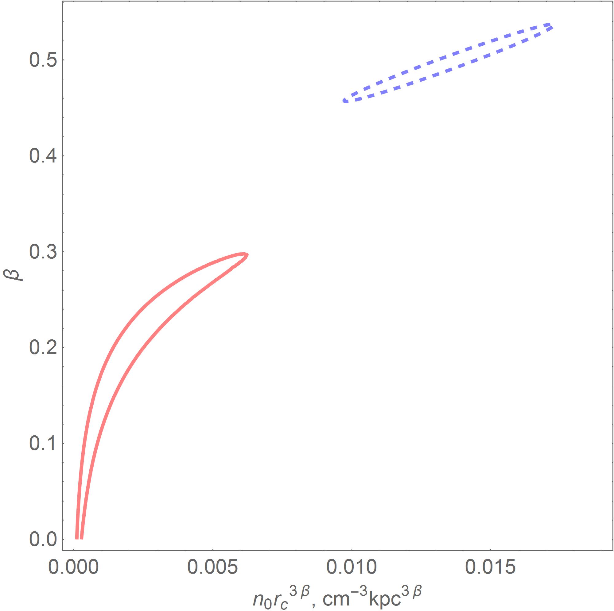
Figure 1: Parameters of the density profile of the circumgalactic gas, Eq. (2), 68% CL contours. Red full line: combination of ram-stripping constraints from nearby Milky-Way satellites (this work, see text). Blue dashed line: combination of X-ray spectroscopic observations assuming $Z=0.3Z_{\odot}$ everywhere (Miller & Bregman, 2015).

2.2 Ram–pressure stripping

Another approach is based on the observation (Blitz & Robishaw, 2000) that the amount of gas in dwarf satellites residing within $\sim 250$ kpc from the centers of the Milky Way and M31 galaxies is much smaller than that observed in more distant dwarfs. This observation is interpreted in terms of the ram-pressure stripping due to travelling of the dwarf galaxies through the circumgalactic gas of their giant companions (see, however, (Emerick et al., 2016), where other potential contributions are discussed). Several constraints on the density of the circumgalactic gas coming from observations of the Milky-Way satellites are collected in Table 1.

	Object	$r$, kpc	$n_{e}$, $10^{-4}$ cm-3	Reference
($+$)	Distant dwarfs	$\langle 0\dots 250\rangle$	$\geq 0.24$	Blitz & Robishaw (2000)
		(volume averaged)
	Carina dwarf	20 (3 …63)	0.85 (0.55 …3.9)	Grcevich & Putman (2009)
	Ursa Minor dwarf	40 (10 …76)	2.1 (0.13 …0.72)
	Sculptor dwarf	68 (31 …83)	2.7 (0.51 …3.9)
(*)	Fornax dwarf	118 (66 …144)	3.1 (0.98 …4.6)
(*)	Sextans dwarf	73.5 (59.8 …90.2)	(1.3 …5)	Gatto et al. (2013)
(*)	Carina dwarf	64.7 (51.2 …81.8)	(1.5 …3.6)
(*)	LMC	48.2$\pm$5	1.1${}^{+0.44}_{-0.45}$	Salem et al. (2015)
($+$)	LMC pulsars	$\langle 0\dots 50\rangle$	$\leq 5$	Anderson & Bregman (2010)
	(dispersion measure)	(line averaged)

Table 1: Direct constraints on the gas density (ram-pressure stripping and pulsar dispersion measures). In the first column, (*) indicates that the constraint was used in the statistical analysis performed in the present work; $(+)$ indicates that this constraint is shown separately in Fig. 4. Round brackets denote uncertainty, angle brackets denote averaging.

The dominant source of uncertainty here is the orbit of a satellite, which determines the pericenter distance, where the stripping is most efficient. To quantify the ensemble of these results, the standard likelihood function, $\mathcal{L}_{s}$, in terms of the two parameters of the gas density distribution, $\beta$ and $n_{0}$, is constructed. Observations with very large uncertainties almost do not affect the result and are not taken into account, see Table 1. The resulting 68% C.L. contour in the parameter space is shown with the full line in Fig. 1. Note that this method constrains the gas density directly, without invoking any assumption on the metallicity. The constraint of Blitz & Robishaw (2000), formulated in a different way (an inequality based on a combined study of a sample of objects, bounding the volume-averaged gas density from below), is not included in the fit. We will return to this constraint in Sec. 3.

2.3 Other constraints

For completeness, recall one more way to constrain the gas density directly. It relies on the observation of pulsar dispersion measures which are related to the column density of electrons along the line of sight. Anderson & Bregman (2010) obtained an upper limit on the electron density integrated up to the LMC, assuming a certain contribution from the inner part of the Milky Way. We will return to this constraint in Sec. 3. Another approach, more robust with respect to assumptions about the inner Galactic gas, was based on individual pulsar studies (Nugaev, Rubtsov & Zhezher, 2016).

3 Combined constraints on the density and metallicity

Figure 1 looks disappointing at first sight since the allowed parameter regions derived in two different approaches do not overlap. However – and this is the main point of the present Letter, – relaxing the assumption of the constant metallicity $Z=0.3Z_{\odot}$ brings them into agreement. Moreover, this opens a possibility to constrain, for the first time, the metallicity profile of the circumgalactic gas from observations.

To proceed further, we determine two likelihood functions corresponding to the two approaches: one is the $\mathcal{L}_{s}(n_{0},\beta)$ determined in Sec. 2.2 and describing constraints from ram-pressure stripping; another one, $\mathcal{L}_{X}$, is responsible for the X-ray constraints. The latter function should depend on parameters of the metallicity profile besides those of the density profile. To quantify this dependence, we assume a similar “beta profile” for the metallicity,

$$Z=A\left(1+\left(r/r_{\rm c}\right)^{2}\right)^{-3B/2}\approx A\left(r/r_{\rm c}\right)^{-3B}.$$ (3)

At large distances from the Galactic Center, a straightforward comparison of Eqs. (1), (2) and (3) results in simple relations between the true $(n_{0},\beta)$ and reported (under assumption of a certain metallicity; $n_{0}^{\prime},\beta^{\prime}$) parameters of the electron densities,

$$n_{0}r_{c}^{3\beta}=\frac{1}{A}n_{0}^{\prime}r_{c}^{3(\beta^{\prime}-B)},$$

$$\beta=\beta^{\prime}-B.$$

This allows one to generalize the likelihood $\mathcal{L}^{\prime}_{X}(n_{0}^{\prime},\beta^{\prime})$ to the more general $\mathcal{L}_{X}(n_{0},\beta,A,B)$. The original $\mathcal{L}^{\prime}_{X}$ function is assumed to be a deformed Gaussian reproducing the 68% C.L. contour of Miller & Bregman (2015), that is the dashed contour in Fig. 1, correctly.

The standard statistical procedure allows one to determine combined constraints on the parameter pairs $(n_{0},\beta)$ and $(A,B)$ by marginalization (see e.g. Cowan (2013)). Let $\mathcal{L}_{e}(n_{0},\beta)$ and $\mathcal{L}_{Z}(A,B)$ be marginalized likelihood functions for the parameters of gas density and metallicity, respectively. Then

$$\mathcal{L}_{Z}(A,B)=\int\!dn_{0}\,d\beta\,\mathcal{L}_{X}(n_{0},\beta,A,B)\mathcal{L}_{s}(n_{0},\beta),$$

$$\mathcal{L}_{e}(n_{0},\beta)=\int\!dA\,dB\,\mathcal{L}_{X}(n_{0},\beta,A,B)\mathcal{L}_{s}(n_{0},\beta).$$

With the help of these new likelihood functions, best-fit values and 68% C.L. contours for combined constraints are easily determined.

Resulting constraints on the metallicity profile, Eq. (3), are shown in Fig. 2.

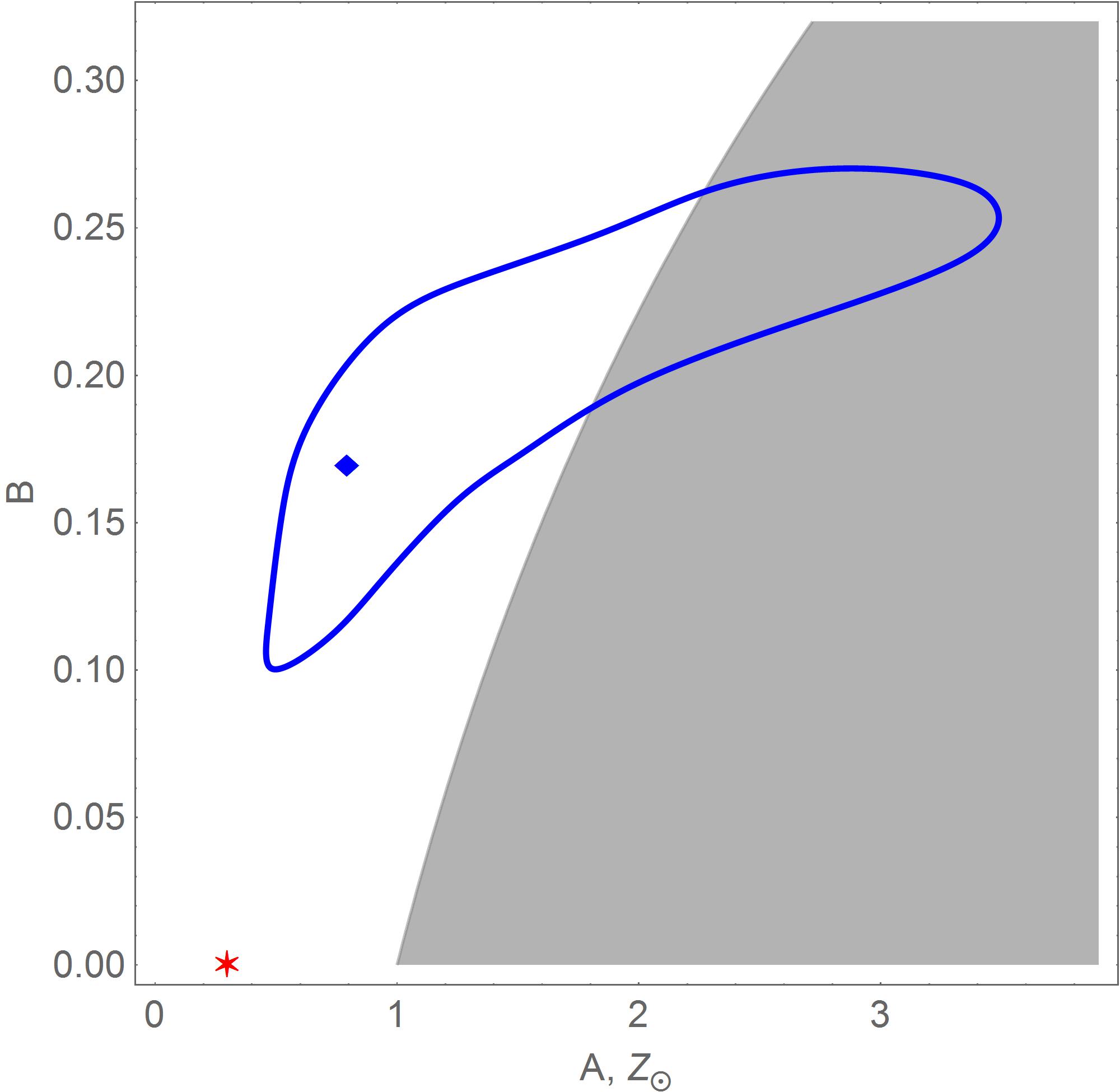
Figure 2: Parameters of the metallicity profile of the circumgalactic gas, Eq. (3). The blue diamond and the blue contour represent, respectively, the best-fit point and the 68% CL contour obtained in this work. The red asterisk gives the values assumed in previous studies. The shaded area corresponds to profiles having $Z(r_{\odot})\geq Z_{\odot}$ for the galactocentric distance of the Sun $r_{\odot}=8.5$ kpc.

The shaded area there corresponds to the parameters resulting in the metallicity at the solar location exceeding $Z_{\odot}$. This information is indicative only since our study deals with the gas at much larger distances from the Galactic Center. The corresponding range of metallicity profiles is shown in Fig. 3.

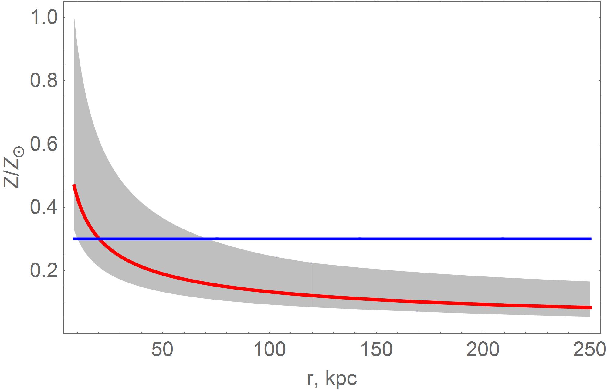
Figure 3: Metallicity profiles of the circumgalactic gas. The red line and the gray shaded area represent, respectively, the best-fit profile and 68% CL allowed range obtained in this work. The blue horizontal line is the constant profile assumed in previous studies.

Figure 4

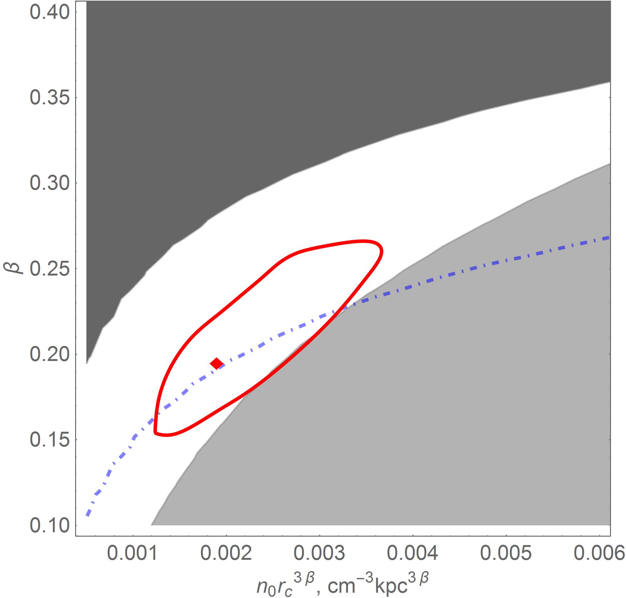
Figure 4: Constraints on the parameters of the density profile of the circumgalactic gas, Eq. (2). The red diamond and the red contour represent, respectively, the best-fit point and the 68% CL contour obtained in this work. The dark shaded area is excluded by Blitz & Robishaw (2000) from studies of the ram-pressure stripping of distant dwarf satellites. The light shaded area is excluded by Anderson & Bregman (2010) from the LMC pulsar dispersion measures. The blue dash-dotted line corresponds to the total mass of the gas of $1.6\times 10^{11}M_{\odot}$ required to explain $\sim 100\%$ of the “missing baryons”.

presents our constraints on the parameters of the density profile, Eq. (2), together with the regions excluded by Blitz & Robishaw (2000) and Anderson & Bregman (2010). Our 68% C.L. allowed region satisfies their constraints. The corresponding range of density profiles is shown in Fig. 5.

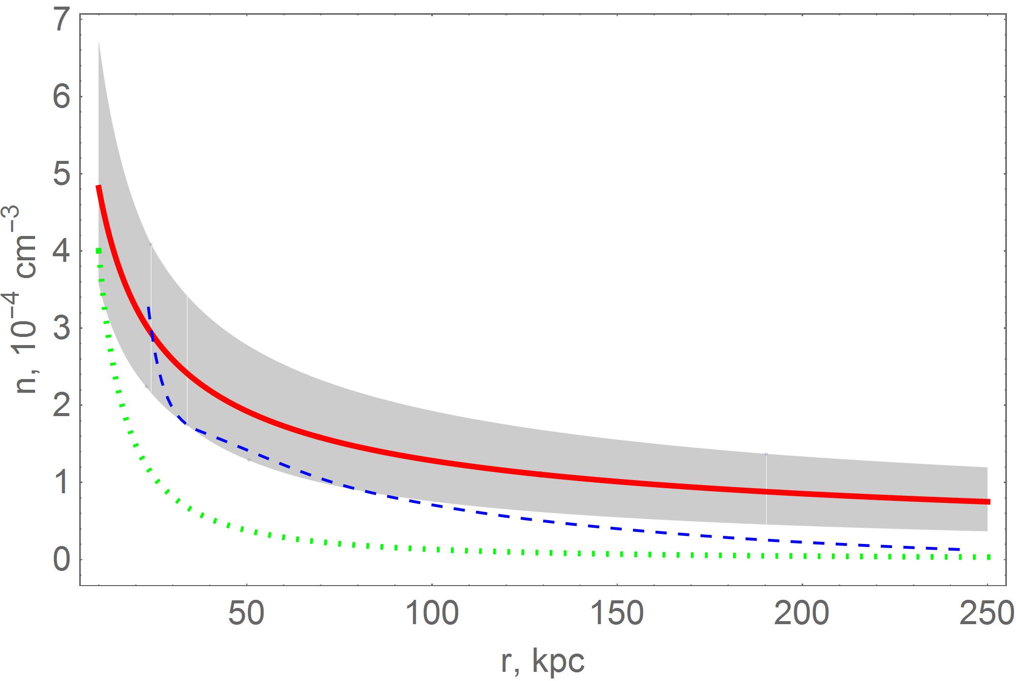
Figure 5: Density profiles of the circumgalactic gas. The red line and the gray shaded area represent, respectively, the best-fit profile and 68% CL allowed range obtained in this work. The green dotted line is the best-fit profile of Miller & Bregman (2015). The blue dashed line is the profile obtained by Feldmann, Hooper & Gnedin (2013) by numerical simulations.

4 Discussion and conclusions

The results of this work eliminate the apparent discrepancy, see Fig. 1, in parameters of the Milky-Way circumgalactic gas estimated from X-ray spectroscopy and from studies of ram-pressure stripping of Galactic dwarf satellites. A combined analysis of the observational constraints, performed here, determines the range of the allowed metallicity profiles of the gas residing up to 250 kpc from the Galactic Center (Figs. 2, 3). Not surprisingly, the metallicity decreases considerably in the outer parts of the halo with respect to the inner part. The profile in the outer part is, however, fairly flat.

Importantly, we obtained constraints on the parameters of the gas density distribution from a combination of all available data (Figs. 4, 5). Compared to the profile of Miller & Bregman (2015), the best-fit one is flatter, resulting in higher gas density in the peripheral parts of the Galactic corona and, consequently, in larger total gas mass. This agrees well with recent simulations (Zheng et al., 2015) and ultraviolet OVI observations (Faerman, Sternberg & McKee, 2016) indicating that the X-ray observations may underestimate the total amount of circumgalactic gas by a factor of two. It is interesting to compare the total gas mass with the “missing baryon” mass of the Galaxy, since the halo of circumgalactic gas was suggested as an explanation of the mismatch between the Milky-Way and cosmological average baryon content (Anderson & Bregman, 2010). One can see from Fig. 4, where a line corresponding to the required “missing-baryon” mass is shown, that our results support this explanation.

It is also interesting to see how our density profile agrees with estimates of the temperature and the luminosity of the Galactic X-ray halo. To this end, we note the relation between the slope parameter $\beta$ in Eq. (2), the velocity dispersion of galactic objects $\sigma$ and the gas temperature $T$,

$$\beta=\frac{\mu m_{p}\sigma^{2}}{kT},$$ (4)

see e.g. Navarro, Frenk & White (1996), where $\mu$ is the mean atomic mass per particle, $m_{p}$ is the proton mass and $k$ is the Boltzmann constant. The velocity dispersion is consistent with $\sigma\sim 100$ km/s in the inner $\sim 80$ kpc (Nesti & Salucii, 2013), but several observations indicate significant decrease of $\sigma$ at large $r$ (Battaglia et. al., 2005; Brown et. al., 2010). We use $\sigma=90$ km/s in the following estimates. The estimated values of $T$ are shown in the right scale of Fig. 6.

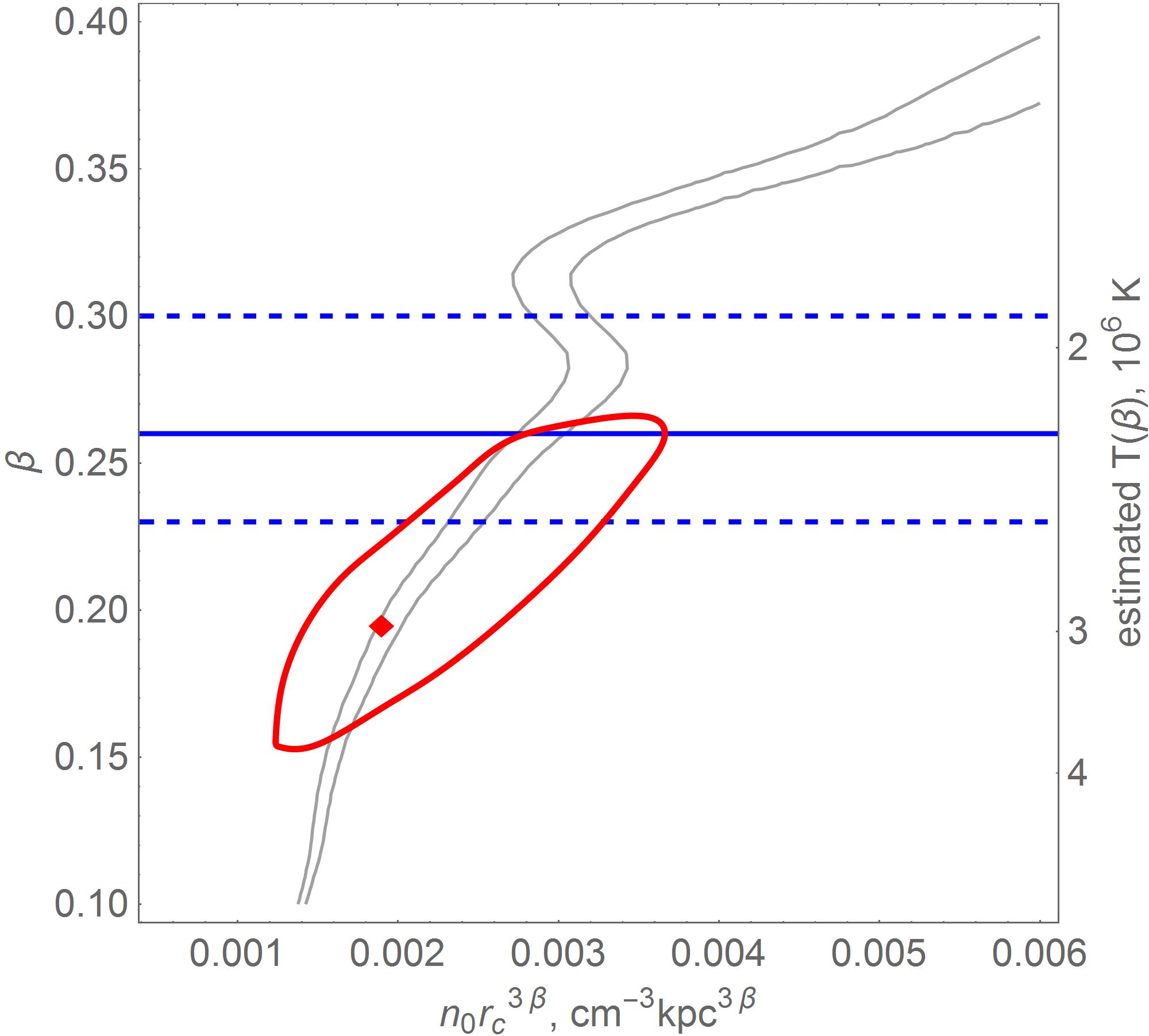
Figure 6: Estimates of the halo temperature $T$ and X-ray luminosity $L_{X}$ versus the density profile parameters. The red diamond and the red contour represent, respectively, the best-fit point and the 68% CL contour obtained in this work. The right scale represents $T$ estimated from $\beta$. Blue horizonthal lines give the $T$ median value (full line, $2.22\times 10^{6}$ K) and interquantile range (dashed lines, $0.63\times 10^{6}$ K) from Henley & Shelton (2013). Thin gray lines bound the range $L_{X}=(2\dots 3)\times 10^{39}$ erg/s favoured by Snowden et al. (1997); Wang (1998). See the text for details and important notes.

Given the approximate nature of these estimates, our density profiles are in a good agreement with observational constraints on the X-ray temperature of the halo gas, for instance, those by Henley & Shelton (2013), shown in Fig. 6. We also calculate the total X-ray luminosity of the halo, $L_{x}$, by making use of Eqns. (17)– (19) of Miller & Bregman (2015). The metallicity enters there through the cooling function (Sutherland & Dopita, 1993) which we take for [Fe/H]$=-1$, corresponding to the most part of the halo, cf. Fig. 3. Observations point to $L_{X}\sim(2\dots 3)\times 10^{39}$ erg/s (Snowden et al., 1997; Wang, 1998), the range shown in Fig. 6 as well, again in a good agreement with our preferred parameters for the density profile.

However, these temperature-related estimates should be considered with caution, because of several reasons. Firstly, the constraints discussed in this paper are relevant for the outer part of the halo, where observational information on X rays is scarce. Secondly, the estimates assume that the halo is isothermal while some studies point to the opposite (Lei, Shelton & Henley, 2009). Thirdly, they assumed constant metallicity and velocity dispersion. Finally, the quantitative values of temperature and luminosity depend on the values of poorly known parameters to which the results of the present paper are insensitive, like $r_{c}$ and $\sigma$, for which we have very little data to work with. Therefore, these considerations and results presented in Fig. 6 should be considered only as a demonstration of the qualitative agreement of our model with observational data on $T$ and $L_{X}$. Indeed, e.g., the replacement of the velocity-dispersion temperature in Eq. (4) by the rotation-curve based temperature estimate would change the gas temperature by a factor of $\sim 2$, indicating a factor of $\sim 2$ higher $\beta$; however, the accuracy of Eq. (4) is of the same order.

Clearly, the beta models themselves might be very crude tools for modelling of the possibly structured circumgalactic gas medium, but relaxing the constant-metallicity assumption and removal of the discrepancies we discuss here are necessary first steps towards understanding of this interesting part of the Galaxy. The gas density profile obtained in this work is considerably flatter than the total mass density profile of the halo, in qualitative agreement with simulations by Feldmann, Hooper & Gnedin (2013). At galactocentric distances $\lesssim 40$ kpc, the profile of Feldmann, Hooper & Gnedin (2013) deviates from the beta profile, Eq. (2), towards higher densities. Unfortunately, this range of distances is not controlled by our approach; therefore, higher densities are not experimentally excluded there.

References

- Anderson & Bregman (2010) Anderson M. E., Bregman J. N., 2010, ApJ, 714, 320
- Battaglia et. al. (2005) Battaglia G. et al., 2005, MNRAS, 364, 433; Erratum: 2006, MNRAS, 370, 1055
- Blitz & Robishaw (2000) Blitz L., Robishaw T., 2000, ApJ, 541, 675
- Brown et. al. (2010) Brown W. R., Geller M. J., Kenyon S. J., Diaferio A., 2010, ApJ, 139, 59.
- Cowan (2013) Cowan G., 2013, arXiv:1307.2487 [hep-ex].
- Emerick et al. (2016) Emerick A., Mac Low M.-M., Grcevich J., Gatto A., 2016, ApJ, 826, 148
- Faerman, Sternberg & McKee (2016) Faerman Y., Sternberg A., McKee C. F., 2016, arXiv:1602.00689.
- Feldmann, Hooper & Gnedin (2013) Feldmann R., Hooper D., Gnedin N. Y., 2013, ApJ, 763, 21
- Gatto et al. (2013) Gatto A., Fraternali F., Read J. I., Marinacci F., Lux H., Walch S., 2013, MNRAS, 433, 2749
- Grcevich & Putman (2009) Grcevich J., Putman M. E., 2009, ApJ, 696, 385; Erratum: 2010, ApJ, 721, 922
- Gupta et al. (2012) Gupta A., Mathur S., Krongold Y., Nicastro F., Galeazzi M., 2012, ApJ, 756, L8
- Henley & Shelton (2013) Henley D. B., Shelton R. L., 2013, ApJ, 773, 92
- Lei, Shelton & Henley (2009) Lei S., Shelton R. L., Henley D. B., 2009, ApJ, 699, 1891
- Miller & Bregman (2013) Miller M. J., Bregman J. N., 2013, ApJ, 770, 118
- Miller & Bregman (2015) Miller M. J., Bregman J. N., 2015, ApJ, 800, 14
- Navarro, Frenk & White (1996) Navarro J. F., Frenk C. S., White S. D. M., 1996, ApJ, 462, 563
- Nesti & Salucii (2013) Nesti F., Salucci P., 2013, JCAP, 1307, 016
- Nugaev, Rubtsov & Zhezher (2016) Nugaev E. Ya., Rubtsov G. I., Zhezher Ya. V., 2016, Astron. Lett., 42, 173
- Salem et al. (2015) Salem M., Besla G., Bryan G., Putman M., van der Marel R. P., Tonnesen, S., 2015, ApJ, 815, 77
- Snowden et al. (1997) Snowden S. L. et al., 1997, ApJ, 485, 125.
- Sutherland & Dopita (1993) Sutherland R. S., Dopita M. A., 1993, ApJS, 88, 253.
- Taylor, Gabici & Aharonian (2014) Taylor A. M., Gabici S. and Aharonian F., 2014, PRD, 89, 103003
- Wang (1998) Wang Q. D., 1998, Lect. Notes Phys., 506, 503
- Zheng et al. (2015) Zheng Y., Putman M. E., Peek J. E. G.. Joung M. R., 2015, ApJ, 807, 103