Collaborative Layer-wise Discriminative Learning in Deep Neural Networks

Abstract

Intermediate features at different layers of a deep neural network are known to be discriminative for visual patterns of different complexities. However, most existing works ignore such cross-layer heterogeneities when classifying samples of different complexities. For example, if a training sample has already been correctly classified at a specific layer with high confidence, we argue that it is unnecessary to enforce rest layers to classify this sample correctly and a better strategy is to encourage those layers to focus on other samples.

In this paper, we propose a layer-wise discriminative learning method to enhance the discriminative capability of a deep network by allowing its layers to work collaboratively for classification. Towards this target, we introduce multiple classifiers on top of multiple layers. Each classifier not only tries to correctly classify the features from its input layer, but also coordinates with other classifiers to jointly maximize the final classification performance. Guided by the other companion classifiers, each classifier learns to concentrate on certain training examples and boosts the overall performance. Allowing for end-to-end training, our method can be conveniently embedded into state-of-the-art deep networks. Experiments with multiple popular deep networks, including Network in Network, GoogLeNet and VGGNet, on scale-various object classification benchmarks, including CIFAR100, MNIST and ImageNet, and scene classification benchmarks, including MIT67, SUN397 and Places205, demonstrate the effectiveness of our method. In addition, we also analyze the relationship between the proposed method and classical conditional random fields models.

1 Introduction

In recent years, deep neural networks (DNNs) have achieved great success in a variety of machine learning tasks [1, 2, 3, 4, 5, 6, 7, 8, 9]. One of the critical advantages contributing to the spectacular achievements of DNNs is their strong capability to automatically learn hierarchical feature representations from a large amount of training data [10, 11, 12, 13], which hence allows the deep models to build sophisticated and highly discriminative features without the harassment of hand-feature engineering. It is well known that deep models learn increasingly abstract and complex concepts from the bottom input layer to the top output layer [14, 15]. Generally, deep models learn low-level features in bottom layers, such as corners, lines and circles, then mid-level features such as textures and object parts in intermediate layers, and finally semantically meaningful concepts in top layers, e.g. the spatial geometry in a scene image [5] and the structure of an object, e.g. a face [16]. In other words, the features learned by deep models, being discriminative for visual patterns of different complexities, are distributed across the whole network.

However, although such a hierarchical property of learned features by deep models has been recognized for a long time, most of existing works [1, 5, 17] only use features from the top output layer and ignore such heterogeneity across different layers. We propose a better policy based on the following consideration: in the task of classifying multiple categories, for many simple input samples, the features represented in bottom or intermediate layers already have sufficient discriminative capability for classification. For example, in the fine-grained classification task, correctly recognizing objects with small intra-class variance like bird species and flower species largely depends on fine-scale and local input features like the color difference and shape distortion, which are easily ignored by top layers because they tend to learn semantic features. Another example is scene classification, where features in the intermediate layer may be sufficiently good for classifying object-centric scene categories, e.g. discriminating a bedroom from other scenes through extracting features around a bed. The top output layer may be inclined to learn the spatial configuration of scenes. Fig. 1 provides more examples. Some recently published works also provide similar observations. Yang et al. [18] showed that different categories of scene images are best classified by features extracted from different layers. In [19], it has been verified that considering mid-level or low-level features increases the segmentation and localization accuracy. However, those works just take features from different layers together and feed the combined features into a single classifier. This strategy may impede the further performance improvement as verified in our experiments due to the introduced redundant information from less discriminative layers.

In this paper, aiming to fully utilize the knowledge distributed in the whole model and boost the discriminative capability of deep networks, we propose a Collaborative Layer-wise Discriminative Learning (CLDL) method that allows classifiers at different layers to work jointly in the classification task. The resulted model trained by CLDL is called CLDL-DNN. Our method is motivated by the following rationale: in training a deep network model, if a sample has already been correctly classified at a specific layer with high confidence, it is unnecessary to enforce the rest layers to focus on classifying this sample correctly and we propose to let them focus on other samples that are not classified correctly yet. More concretely, to implement this idea, we introduce multiple classifiers on top of multiple layers. Each classifier not only tries to correctly classify the features from its input layer, but also coordinates with other classifiers to jointly maximize the final classification performance. Guided by the other companion classifiers, each classifier learns to concentrate on certain training examples. Classifying samples at different layers can boost the performance of the model. Interestingly, we demonstrate that the CLDL method is similar to constructing a conditional random field (CRF) [20] across multiple layers. In practice, the proposed CLDL can be easily incorporated into most neural network architectures trained using back propagation. We experimentally verify the superiority of our method, achieving state-of-the-art performance using various deep models, including NIN, GoogLeNet and VGGNet on six heavily benchmarked datasets for object classification and scene classification tasks.

The rest of this paper is organized as follows. Section 2 reviews the related work. Detailed descriptions of CLDL is given in Section 3. Experiments and discussions are presented in Section 4 and Section 5 concludes the paper.

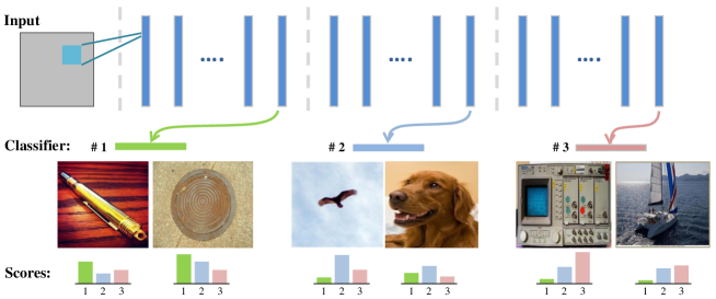
Figure 1: Examples from ImageNet dataset showing that features from different layers in a deep network are good at discriminating images of different complexities. Three collaborative classifiers are introduced at different layers of a deep model using our proposed CLDL method. The input images in the middle row are with increasing complexity from left to right. The bottom row shows the prediction scores of corresponding images on the ground truth category produced by classifiers in CLDL. One can find that classifiers introduced at bottom/top layers of a deep model can correctly classify simple/complex samples. Note that classifiers with a smaller index number lie at lower-level layers. All figures in this paper are best viewed in color.

2 Related Work

Since Krizevsky et al. [1] demonstrated the dramatic performance improvement by deep networks in ImageNet competition, deep networks have achieved exciting success in various computer vision and machine learning tasks. Many factors are thought to contribute to the success of deep learning, such as availability of large-scale training datasets [21, 5], deeper and better network architectures [4, 17, 22], development of fast and affordable parallel computing devices [23], as well as a large number of effective techniques in training large-scale deep networks, such as ReLU [24] and its variants [25, 26], dropout [27], and data augmentation [1]. Here we mainly review existing works that leverage multi-scale features learned at different layers of a deep model and multiple objective functions to improve the classification performance.

Combining Multi-Scale Features It is widely known that different layers in a deep neural network output features with different scales that represent the input data of various abstractness levels. To boost the performance of deep networks, a natural idea is to combine the complementary multi-scale features. Long et al. [3] proposed to combine the features from multiple layers and used the features to train a CRF for semantic segmentation. Based on [3], Xie et al. [28] used multi-scale outputs of a deep network to perform edge detection. Hypercolumn [19] used the activations of CNN units at the same location across all layers as features to boost performance in segmentation and fine-grained localization. Similarly, DAG-CNN [18] proposed to add prediction scores from multiple layers as the final score in image classification. Different from the above methods, our proposed CLDL method not only utilizes multi-scale features by building classifiers on top of different layers, but also encourages each classifier to automatically learn to specialize on training patterns and concepts with certain abstractness during the collaborative training. CLDL thus can effectively improve the overall discriminative capability of the network.

Combining Multiple Objective Functions Some recent works propose to combine multiple objective functions to train a deep model. In [29], several loss functions were appended to the output layer of a deep network as regularizers to reduce its risk of overfitting. DSN [30] proposed to add a “companion” hinge-loss function for each hidden layer. Although the issue of “vanishing gradient” in training can be alleviated, it is hard to evaluate the contributions of the trained classifiers at hidden layers in DSN since only the classifier at the output layer is used in testing. GoogLeNet [22] introduced classifiers at two hidden layers to help speed up convergence when training a large-scale deep network, and only used the classifier at the top output layer to do inference. Different from the above methods, we propose a collaborative objective function for multiple classifiers on different layers, each of which coordinates with others to jointly train a deep model and classify a new testing sample. A recent work of LCNN [31] aimed to improve the discriminability of the late hidden layer by forcing each neuron to be activated for a manually assigned class label. In contrast, our method has a stronger discriminative capability by enabling each hidden layer to automatically learn to be discriminative for certain data without human interference.

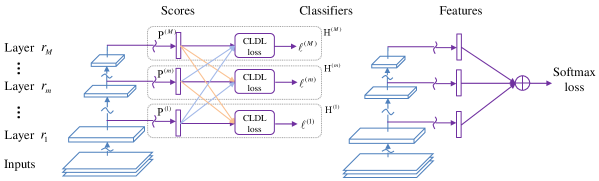
Figure 2: Comparisons on architectures of our proposed CLDL-DNN and related work [18, 19]. The symbol “$\sim$” represents hidden layers. Left: CLDL-DNN. Multiple classifiers ${\rm H}^{(1)},\ldots,{\rm H}^{(M)}$ are introduced at different layers. With the CLDL loss (ref. Eqn. (1)), each classifier is fed with the prediction scores from all other classifiers. We also introduce a simplified version of CLDL, i.e. CLDL- in Section 3.5 by removing the feedback connections (orange lines). Right: The architecture used in Hypercolumn [19] and DAG-CNN [18]. Multi-scale features extracted at multiple layers are simply taken together and fed into a classifier, which has conventional loss functions, e.g. softmax loss. All notations in this figure are defined in the text of Section 3.1.

3 Collaborative Layer-wise Discriminative Learning

In this section, we introduce our proposed CLDL method in details. Firstly, we describe the motivation and definition of CLDL. Secondly, we introduce the training and testing strategies of deep models using CLDL. Thirdly, we explain the rationales for CLDL. Fourthly, we give understanding on CLDL by establishing its relation with classic conditional random fields (CRF) [20]. Finally, we explore variants of CLDL in order to gain a deeper understanding of CLDL.

3.1 Motivation and Definition of CLDL

The proposed collaborative layer-wise discriminative learning (CLDL) method aims to enhance the discriminative capability of deep models by learning complementary discriminative features at different layers such that each layer is specialized for classifying samples of certain complexities. CLDL is motivated by the widely recognized fact that the intermediate features learned at different layers in a deep model are suitable for discriminating visual patterns of different complexities. Therefore, encouraging different layers to focus on categorizing input data of different properties, rather than forcing each of them to address all the data, one can improve layer-level discriminability as well as final performance for a deep model. In other words, with this strategy, the knowledge distributed in different layers of a deep network can be effectively utilized and the discriminative capability of the overall deep model is largely enhanced by taking advantage of those discriminative features learned from multiple layers.

We now give necessary notations to formally explain CLDL. For brevity, we only consider the case of one training sample, and the formulation for the multiple samples case can be derived similarly since samples are independent. We denote a training sample as $(\mathbf{x},y^{*})$ where $\mathbf{x}\in R^{d}$ denotes the raw input data, $y^{*}\in\{1,\ldots,K\}$ is its ground truth category label and $K$ is the number of categories.We consider a deep model consisting of $L$ layers, each of which outputs a feature map denoted as ${\mathbf{X}}^{(l)}$. Here ${\mathbf{X}}^{(0)}$ and ${\mathbf{X}}^{(L)}$ represent the input and final output of the network, respectively. $\mathbf{W}^{(l)}$ denotes the parameter of filters or weights to be learned in the $l$-th layer. Using above notations, the output of a $L$-layer deep network at each layer can be written as

$$\footnotesize\mathbf{X}^{(l)}=f^{(l)}(\mathbf{W}^{(l)}*\mathbf{X}^{(l-1)}),\ \ l=1,\ldots,L\,\ \ \text{and}\ \ \mathbf{X}^{(0)}\triangleq\mathbf{x},\vspace{-2mm}$$

where $f^{(l)}(\cdot)$ is a composite of multiple specific functions including activation function, dropout, pooling and softmax. For succinct notations, the bias term is absorbed into $\mathbf{W}^{(l)}$.

CLDL chooses $M$ layers out of the $L$ layers which are indexed by $S=\{r_{m},m=1,\ldots,M\}$, $r_{m}\in\{1,\ldots,L\}$ and places classifiers on each of the layers. Denote each classifier as ${\rm H}^{(m)}$ and the classifier set excluding ${\rm H}^{(m)}$ as ${\rm\bar{H}}^{(m)}$. ${\rm H}^{(m)}$ outputs categorical probability scores $\mathbf{P}^{(m)}=(\mathbf{P}^{(m)}(1),\ldots,\mathbf{P}^{(m)}(K))$ over all $K$ categories. Note that we have $\left\|{\mathbf{P}^{(m)}}\right\|_{1}=1$ since $\mathbf{P}^{(m)}$ denotes a probability distribution. When the classifier ${\rm H}^{(m)}$ has high confidence in classifying the input data $\mathbf{X}^{(0)}$ to the category $y^{*}$, the value of $\mathbf{P}^{(m)}(y^{*})$ will be close to 1. The CLDL loss function for ${\rm H}^{(m)}$ is defined as

$$\ell^{(m)}(\mathbf{x},y^{*},\mathcal{W}) =-\log\mathbf{P}^{(m)}(y^{*})\prod\limits_{\scriptstyle t=1,\scriptstyle t\neq m}^{M}{[1-\mathbf{P}^{(t)}(y^{*})]^{\frac{1}{{M-1}}}},$$ (1)

$$\footnotesize\mathbf{P}^{(m)}(y^{*}) =h^{(m)}_{y^{*}}(\mathbf{w}^{(m)},\mathbf{X}^{(r_{m})}),$$ (2)

where $h^{(m)}_{y^{*}}(\mathbf{w}^{(m)},\mathbf{X}^{(r_{m})})$ denotes the mapping function of the classifier ${\rm H}^{(m)}$ from input feature $\mathbf{X}^{(r_{m})}$ to category label $y^{*}$, and $\mathbf{w}^{(m)}$ is the parameters associated with ${\rm H}^{(m)}$. $\mathcal{W}$ is defined as all the learnable weights in CLDL:

$$\footnotesize{\mathcal{W}}=({\bf{W}}^{(1)},\ldots,{\bf{W}}^{(L)},{\bf{w}}^{(1)},\ldots,{\bf{w}}^{(M)}).\vspace{-2mm}$$

For better understanding, we further divide the loss function in Eqn. (1) into multiplication of two terms as

$$\footnotesize\ell^{(m)}=T^{(m)}C^{(m)},$$ (3)

$$\footnotesize T^{(m)}=\prod\limits_{\scriptstyle t=1,\scriptstyle t\neq m}^{M}{[1-{\mathbf{P}}^{(t)}(y^{*})]^{\frac{1}{{M-1}}}},\ \ \ \ \ \ C^{(m)}=-\log{\mathbf{P}^{(m)}}(y^{*}).\vspace{-1mm}$$ (4)

Here, $T^{(m)}$ carries modulation message collaborating with the classifier ${\rm H}^{(m)}$, and $C^{(m)}$ is the confidence output by ${\rm H}^{(m)}$ (we discuss the roles of $T^{(m)}$ and $C^{(m)}$ in more details later). Note that ${\rm H}^{(m)}$ employed in our method can be chosen freely from many kinds of conventional classifiers to satisfy the requirements of different tasks, including neural network [32], SVM [33], and logistic regression classifier [34], etc. The architecture of CLDL-DNN is illustrated in Fig. 2.

3.2 Training and Testing Strategies for CLDL

The overall objective function of CLDL is a weighted sum of loss functions from all classifiers, with a weight decay term to control complexity of the model:

$$\footnotesize L^{(\text{Net})}(\mathbf{x},y^{*},\mathcal{W})=\sum\limits_{m=1}^{M}{\lambda_{m}\ell^{(m)}}+\mathbf{\alpha}\left\|{\mathcal{W}}\right\|_{2},\vspace{-1.5mm}$$

where $\mathbf{\alpha}\in R^{+}$ is the penalty factor which is set to be the same for all learnable weights for simplicity, and $\lambda_{m}\in R^{+}$ denotes the weight of each classifier, used to balance the effect of the corresponding classifier in the overall objective function. The goal of training is to optimize all the learnable weights:

$$\footnotesize\mathcal{W}^{*}=\mathop{\arg\min}\limits_{\mathcal{W}}L^{(\text{Net})}(\mathbf{x},y^{*},\mathcal{W}).$$

The network can be trained in an end-to-end manner by standard back-propagation, and the gradient for variables of the $l$-th layer $Q^{(l)}\in\{\mathbf{X}^{(l)},\mathbf{W}^{(l)},\mathbf{w}^{(l)}\}$ is calculated by following the chain rule which leads to

$$\frac{{\partial L^{(\text{Net})}}}{{\partial Q^{(l)}}} =\sum\limits_{m=1}^{M}{\lambda_{m}\frac{{\partial\ell^{(m)}}}{{\partial Q^{(l)}}}}+{\bf{\alpha}}\frac{{\partial\left\|{\mathcal{W}}\right\|_{2}}}{{\partial Q^{(l)}}}=\sum\limits_{m=1}^{M}{\lambda_{m}\frac{{\partial C^{(m)}}}{{\partial Q^{(l)}}}}T^{(m)}+{\bf{\alpha}}\frac{{\partial\left\|{\mathcal{W}}\right\|_{2}}}{{\partial Q^{(l)}}},$$ (5)

$$\frac{{\partial\ell^{(m)}}}{{\partial{\bf{X}}^{(l)}}} =\begin{cases}\frac{-1}{{\mathbf{P}^{(m)}(y^{*})}}\frac{{\partial h_{y^{*}}^{(m)}}}{{\partial\mathbf{X}^{(r_{m})}}}\frac{{\partial f^{(r_{m})}(\mathbf{W}^{(r_{m})}*\mathbf{X}^{(r_{m}-1)})}}{{\partial\mathbf{X}^{(l)}}}{T}^{(m)},&l<r_{m}\\ \frac{-1}{{\mathbf{P}^{(m)}(y^{*})}}\frac{{\partial h_{y^{*}}^{(m)}}}{{\partial\mathbf{X}^{(r_{m})}}}T^{(m)},&l=r_{m}\\ 0,&l>r_{m}.\\ \end{cases}$$ (6)

Recall $r_{m}$ is the index of the input layer for ${\rm H}^{(m)}$. The loss $\ell^{(m)}$ only contributes to optimizing the layers lying on the input layer of ${\rm H}^{(m)}$. Here,

$$\footnotesize\frac{{\partial\ell^{(m)}}}{{\partial\mathbf{W}^{(l)}}} =\frac{{\partial\ell^{(m)}}}{{\partial\mathbf{X}^{(r_{m})}}}\frac{{\partial f^{(r_{m})}(\mathbf{W}^{(r_{m})}*\mathbf{X}^{(r_{m}-1)})}}{{\partial\mathbf{W}^{(l)}}}+2\alpha,l<r_{m},$$ (7)

$$\footnotesize\frac{{\partial\ell^{(m)}}}{{\partial\mathbf{w}^{(l)}}} =\frac{-1}{{\mathbf{P}^{(m)}(y^{*})}}\frac{{\partial h_{y^{*}}^{(m)}}}{{\partial\mathbf{w}^{(l)}}}T^{(m)}+2\alpha.$$ (8)

In gradient calculation, we treat $T^{(m)}$ as independent of $Q^{(l)}$ during the error back-propagation w.r.t. $Q^{(l)}$. Therefore, we set $\frac{{\partial T^{(m)}}}{{\partial Q^{(l)}}}=0$. In this way, $T^{(m)}$ acts as a weight factor which is related with the prediction scores output by classifiers in ${\rm\bar{H}}^{(m)}$ and it controls the scale of the gradients calculated for updating ${\rm H}^{(m)}$. The advantages of such simplification are two-fold. Firstly, calculation of gradients becomes easy and fast, and meanwhile the numerical problem in calculating $\frac{{\partial T^{(m)}}}{{\partial Q^{(l)}}}$ when $\mathbf{P}^{(s)}(y^{*})$ for $s\in\{1,\ldots,M\}$ but $s\neq m$ is close to 1 can be avoided (see Supplementary Materials for further details). Secondly, it reduces the risk of overfitting, which has been empirically verified and can be explained by seeing $\frac{{\partial T^{(m)}}}{{\partial Q^{(l)}}}=0$ as a regularizer. In practice, given the function forms of ${h_{y^{*}}^{(m)}}$ and $f^{(l)}$, it is easy to calculate necessary gradients according to Eqn. (5)-(8).

In the training phase, we in fact optimize learn-able weights through a maximum likelihood estimation (MLE) as follows:

$$\footnotesize{\mathcal{W}}^{*}=\mathop{\arg\max}\limits_{\mathcal{W}}P(y^{*}|\mathbf{x},{\mathcal{W}})=\mathop{\arg\min}\limits_{\mathcal{W}}L^{(\text{Net})}(\mathbf{x},y^{*},\mathcal{W}),$$

where the likelihood distribution is parameterized by a deep network. To be consistent with the training, in the testing phase, we do inference to decide the most probable class label by solving the discrete optimization problem

$$\footnotesize y^{*}=\mathop{\arg\max}\limits_{y}P(y|\mathbf{x},\mathcal{W})=　\mathop{\arg\min}\limits_{y}L^{(\text{Net})}(\mathbf{x},y,\mathcal{W}),$$ (9)

where $y\in\{1,\ldots,K\}$. Similarly, it is easy to predict the top $k$ categories for the input data using Eqn. (9).

3.3 Explanations on CLDL

In the following, we explain how the CLDL enhances the discriminative capability of a deep network.

As shown in Eqn. (3), the loss function of each classifier considers two multiplicative terms, i.e. $T^{(m)}$ and $C^{(m)}$. Here, $C^{(m)}$, taking the form of entropy loss [35], depicts the predicted confidence for the sample belonging to a specific category. Minimizing $C^{(m)}$ pushes the classifier ${\rm H}^{(m)}$ to hit its ground truth category. $T^{(m)}$ is a geometric mean of the prediction scores on the target class output by other classifiers in ${\rm\bar{H}}^{(m)}$. $T^{(m)}$ measures how well those “companion” classifiers perform on classifying the input sample. Here comes the layer-wise collaboration (or competition). When the input sample is correctly classified by all classifiers in $\rm\bar{H}^{(m)}$, the value of $T^{(m)}$ is small; otherwies, $T^{(m)}$ takes a large value. Considering $T^{(m)}$ together with $C^{(m)}$ distinguishes our CLDL loss function from conventional loss functions: in CLDL, each classifier considers performance of other classifiers in the same network when trying to classify a input sample correctly. The classifier will put more efforts on the samples difficult for other classifiers and care less about samples that have been addressed well by other classifiers. As a result, the optimization of CLDL can be deemed as a collaborative learning process. All classifiers share a common goal: maximizing the overall classification performance by paying attention to different subsets of the samples. In more details, by using CLDL we encourage the deep network to act in following ways.

• If all classifiers in ${\rm\bar{H}}^{(m)}$ have correctly classified input data $\mathbf{x}$, we have $\mathbf{P}^{(t)}(y^{*})$ close to 1, for $t=1,\ldots,M$, but $t\neq m$. Hence $T^{(m)}$ takes a small value close to 0. According to Eqn. (5)-(8), the gradients on learnable weights $\mathcal{W}$ that are back propagated from classifier ${\rm H}^{(m)}$ are suppressed by small $T^{(m)}$. In other words, the classifier ${\rm H}^{(m)}$ at layer $r_{m}$ need not correctly predict $\mathbf{x}$ as it is informed that $\mathbf{x}$ has already been classified correctly by other classifiers. Therefore, the risk of overfitting to these samples for ${\rm H}^{(m)}$ is reduced.

• If no classifier in ${\rm\bar{H}}^{(m)}$ correctly predicts the category of the input $\mathbf{x}$, $T^{(m)}$ would have a large value close to 1. According to Eqn. (5)-(8), ${\rm H}^{(m)}$ will be encouraged to focus on learning this sample that is difficult for other classifiers. The hard sample may be well discriminated using the features of ${\rm H}^{(m)}$ at a proper level of feature abstraction.

• If ${\rm\bar{H}}^{(m)}$ is a mixture of classifiers, some of which correctly classify the input and some cannot. Then one can see that the value of $T^{(m)}$ is positively correlated with the prediction score of ${\rm H}^{(m)}$ on the ground truth category (see Supplementary Materials for rigorous derivations). Thus the classifier with the highest prediction score will dominate the updating of the weights. In this way, we encourage the classifier with the best discriminative capability to play the most important role in learning from the input data.

We also note that other methods that add conventional classifiers on multiple layers, e.g. GoogLeNet [22] and DSN [30] can be viewed as special cases of our method by setting $T^{(m)}$ as a constant 1 and the values of $\lambda_{m}$ for classifiers at hidden layers as 0 in testing. In [22, 30], since no classifier stays informed of the output of other classifiers, every classifier is forced to fit all of the training data and ignores the different layer-wise discriminative capabilities to different input data. One disadvantage of such a strategy is that classifiers would be prone to overfitting, thus hampering the discriminability of the overall model. In contrast, by focusing on learning from certain samples, classifiers in CLDL reduce the risk of overfitting over the whole training set and have a better chance to learn more discriminative representations for the data.

3.4 Discussions on Relation Between CLDL and CRF

In this subsection, we demonstrate that CLDL can be viewed as a simplified version (with higher optimization efficiency) of a conditional random field (CRF) model.

CRF is an undirected graphical discriminative model that compactly represents the conditional probability of a label set $Y=\{y^{*}_{1},\ldots,y^{*}_{n}\}$ given a set of observations $X=\{\mathbf{x}_{1},\ldots,\mathbf{x}_{n}\}$, i.e. $P(Y|X)$. In CLDL, we introduce another hidden label set $S=\{s_{1},\ldots,s_{n}\}$ to be the assignment of each $\mathbf{x}_{i}\in X$ to a certain classifier ${\rm H}^{(m)}$. $s_{i}$ takes its value from $\{1,\ldots,M\}$. Recall $M$ is the number of classifiers in CLDL. In our classification scenario, given a training set $\{(\mathbf{x}_{1},y^{*}_{1}),\ldots,(\mathbf{x}_{n},y^{*}_{n})\}$, optimizing $P(Y|X)=\sum_{S}P(Y|X,S)P(S|X)$ w.r.t the weight parameter gives a CRF model that distributes $n$ observations into $M$ classifiers with an optimal configuration in the sense of maximizing the training accuracy.

More concretely, the conditional probability specified in our CRF model can be written as

$$\footnotesize P(S|X)=\frac{1}{Z}\exp(\beta^{\top}f(S,X)),$$

where $Z$ is a partition function and $\beta$ is the weight parameter. Following the notations given in Eqn. (2), the function $f(S,X)$ in our CLDL case is specifically defined as

$$\footnotesize f(S,X)=\left[\log\left(1-h_{y_{i}}^{1}({\bf w}^{(1)},\mathbf{X}^{(r_{1})})\right),\ldots,\log\left(1-h_{y_{i}}^{M}({\bf w}^{(M)},\mathbf{X}^{(r_{M})})\right)\right]^{\top},\vspace{-2mm}$$

and each element of the weight parameter $\beta$ takes a fixed value $\frac{1}{M-1}$.

Then the likelihood $P(Y|X)$ is given by classifiers associated with the layers indicated by $S$. Here, $P(Y|X,S)$ is parameterized by the chosen classifier as indicated in Eqn. (2): $P(y^{*}|\mathbf{x},s)=h^{(s)}_{y^{*}}({\mathbf{w}}^{(s)},\mathbf{X}^{(r_{s})})$. Maximizing $P(Y|X)$ gives the optimal value of the assignment indicator $s$ for $\bf x$ as well as the classifier parameter ${\bf w}^{(s)}$ for each collaborative classifier.

CRF can be solved via a standard message passing algorithm. In CLDL, we simplify the CRF into a chain and apply error back propagation for optimization.

3.5 Variants of CLDL

To further verify the effectiveness of CLDL, we have also explored an alternative method to utilize the layer-level discriminative information and we here compare it with CLDL.

This method we explore is called CLDL- and can be seen as a simplification of CLDL. As indicated in Fig. 2, its only difference from CLDL lies in that there is no feedback connection from classifiers at top layers to classifiers at bottom layers. More concretely, in the definition of $T^{(m)}$ for CLDL-, which is formulated by $T^{(m)}=\prod\limits_{t=1}^{m-1}{(1-{\bf P}^{(t)}(y^{*}))^{\frac{1}{{m-1}}}}$, we can see that the information flow among different classifiers takes a single direction: the classifiers on top layers can get the prediction scores from classifiers on bottom layers, but the reverse does not hold. This is similar to the cascading strategy used in face detection [36]. The advantage of CLDL over CLDL- is that each classifier is able to automatically focus on learning to categorize certain examples by taking all other classifiers’ behavior into optimization. Therefore, CLDL demonstrates better discriminative capability than CLDL-, which is empirically verified in the experiment part.

4 Experiments and Analysis

4.1 Experimental Setting

To evaluate our method thoroughly, we conduct extensive experiments for two classification tasks, i.e. object classification on CIFAR-100 [37], MNIST [38] and ImageNet [21] datasets, and scene classification on MIT67 [39], SUN397 [40] and Places205 [5] datasets. There are overall three state-of-the-art deep neural networks with different architectures tested on these datasets, including NIN [41], GoogLeNet [22] and VGGNet [17]. Specifically, NIN is used on CIFAR-100 and MNIST, GoogLeNet is used on ImageNet and VGGNet is used on scene recognition tasks. All of these deep models have achieved state-of-the-art performance on the datasets we use. We choose Caffe [42] as the platform to train different models and conduct our experiments. To reduce the training time, four NVIDIA TITAN X GPUs are employed in parallel for training.

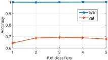
Figure 3: Evaluations of NIN model on CIFAR-100 for investigating the effect of classifier number in CLDL on the classification accuracy for both training and validation sets. Left: classification accuracy curves without data augmentation. Right: classification accuracy curves with data augmentation.

4.2 Deciding Position and Number of Classifiers

Before applying CLDL in practice, an important problem one needs to solve is to determine which layers to put the collaborative classifiers. Analytically solving this problem is hard. Therefore, we propose a simple yet effective heuristic method to determine the proper position and number of classifiers. From top output layer to bottom input layer, we place a classifier every $V$ weight layers and $V$ is calculated by $V=\left\lceil{\left(L/M\right)^{\gamma}}\right\rceil$, in which $L$ and $M$ follow the notations in Section 3.1. Accordingly, indexes of layers to put classifiers are calculated by $r_{m}=L-(M-m)V$, $m\in{1,\ldots,M}$. Throughout our experiments, we set $\gamma<1$ (here $\gamma=0.8$) to suppress the value of $V$. In this way, one can avoid placing classifiers at very bottom layers when the number of classifiers is large, because very bottom layers describe basic concepts and should be shared among all categories. To test the influence of various numbers of collaborative classifiers in CLDL on the final performance, we conduct primitive experiments on CIFAR100 with data augmentation using different numbers of classifiers ($M=1,2,3,4,5$). When $M=1$, we are actually using a single softmax classifier on top of the network. The experimental results are shown in Fig. 3, from which one can observe that the performance increases with more classifiers added (when $M=1,2,3$) at the beginning, and then decreases if we continue adding more classifiers (when $M=4,5$). This phenomenon could be explained as follows: when the number of classifiers is small, the deep network can benefit from various discriminative information in different layers, but the network will gain little from too many classifiers added because neighboring layers often contain redundant information with each other. Finally, the performance on the validation set will drop due to overfitting. Based on the conclusion from this experiment, in the following experiments, we set $M=3$ for all the datasets. Note that more careful tuning on the number of classifiers for different datasets might further improve the performance of CLDL. Nevertheless, we show that state-of-the-art performance has been achieved using the same configuration.

In our experiments, three kinds of deep models including NIN, GoogLeNet and VGGNet are used as base models to evaluate the performance of CLDL on different datasets. We denote those three models trained with CLDL as CLDL-NIN, CLDL-GoogLeNet and CLDL-VGGNet, respectively. The positions of classifiers are in line with the calculation of $r_{m}$. In CLDL-NIN, each classifier consists of a mlpconv layer [41] to output feature maps with the same number of channels as the number of categories, and global averaging pooling layer [41] to transform the size of the feature map into $1\times 1$. In CLDL-GoogLeNet, we just simply replace the softmax loss function in each classifier with CLDL loss function given in Eqn. (1) without changing the rest network structure. By doing so, the results of CLDL-GoogLeNet can show more clearly the effects of CLDL on a deep model. In CLDL-VGGNet, similar to previous methods such as [18, 19], we use two fully connected layers in our classifiers. Throughout experiments, we set $\lambda_{1}=\lambda_{2}=0.3,\lambda_{3}=1$.

Table 1: Classification error rates on CIFAR-100 either when data augmentation is used or not. d.a. represents “data augmentation”. Note since there is no reported result on CIFAR-100 using data augmentation in NIN [41], we refer to the results reimplemented by [43] (denoted by NIN^∗). All tespts are by single model and single crop.

Model	Without d.a. (%)	With d.a. (%)
Maxout [44]	38.57	-
Prob maxout [45]	38.14	-
Tree based priors [46]	36.85	-
CNN + Maxout [47]	-	34.54
dasNet [47]	-	34.50
NIN [41]	35.68	-
NIN∗ [43]	35.96	32.75
APL [43]	34.40	30.83
DSN [30]	34.57	-
$\rm{DSN}^{*}$-NIN (ours)	34.12	32.95
CLDL--NIN (ours)	31.27	30.41
CLDL-NIN (ours)	30.40	29.05

Table 2: Classification error rates on MNIST. All tests are by single model and single crop.

Model	Error rate (%)
Stochastic Pooling [48]	0.47
Maxout [44]	0.47
NIN [41]	0.42
DSN [30]	0.39
CLDL-NIN (ours)	0.28

Table 3: Top-5 classification error rates on ImageNet. Tests for CLDL-GoogLeNet are by single model and single crop.

Model	Top-5 (%)
AlexNet [1]	15.4
ZF [49]	13.51
LCNN [31]	12.91
GoogLeNet [22]	11.1
CLDL-GoogLeNet (ours)	10.21

4.3 Results for Object Classification

We now apply CLDL to object recognition on the following three benchmark datasets. All of our models using CLDL are trained from scratch.

4.3.1 CIFAR-100

The CIFAR-100 dataset contains 50,000 and 10,000 color images with size of $32\times 32$ from 100 classes for training and testing purposes, respectively. Following [44], preprocessing including global contrast normalization and ZCA whitening is applied. The comparison results of CLDL-NIN with other state-of-the-art models with and without data augmentation are shown in Table 1, from which we can see that CLDL-NIN achieves the best performance against all the compared methods.

Specifically, CLDL remarkably outperforms the baseline model (NIN) by reducing the error rates by 5.56%/3.70% with/without data augmentation, demonstrating the effectiveness of CLDL in enhancing the discriminative capability of deep models. Compared with DSN, which imposes independent classifiers on each hidden layer of NIN, CLDL-NIN reduces the error rate by 4.17% when no data augmentation is used. Furthermore, we replace the loss function of each classifier in CLDL-NIN by conventional softmax loss function, which gives $\rm{DSN}^{*}$-NIN. We train $\rm{DSN}^{*}$-NIN using the training methods for DSN. By comparing the performance of CLDL-NIN and $\rm{DSN}^{*}$-NIN, we can see CLDL-NIN achieves lower error rates either when data augmentation is used or not. This clearly proves that our method has superiority on improving the discriminative capability of the deep model and alleviating overfitting (both models achieve nearly 100% accuracy on the training set) through allowing the classifiers to work collaboratively. Besides, compared with CLDL-, CLDL-NIN further reduces the error rates by 0.87%/1.36% with/without data augmentation, proving the advantages of CLDL over CLDL-.

4.3.2 MNIST

MNIST is a heavily benchmarked dataset, which contains 70,000 28$\times$28 gray scale images of numerical digits from 0 to 9, splitting into 60,000 images for training and 10,000 images for testing. On this dataset, we apply neither any preprocessing to the image data nor any data augmentation method, both of which may further improve the performance. A summary of best methods on this dataset is provided in Table 3, from which one can again observe that CLDL-NIN performs better than other methods with a significant margin.

4.3.3 ImageNet

To test the scalability of our method to a large number of classes and deeper networks, we evaluate the CLDL method with a much more challenging and larger-scale 1000-class ImageNet dataset, which contains roughly 1.2 million training images, 50,000 validation images and 100,000 test images. Our baseline model is the GoogLeNet, which has reported the best performance on image classification in the ImageNet competition in 2014 [49]. We train CLDL-GoogLeNet from scratch using the publicly available configurations released by Caffe in Github¹. On this dataset, no additional preprocessing is used except subtracting the image mean from each input raw image.

Table 3 summarizes the performance of CLDL-GoogLeNet and other deep models on the validation set of ImageNet. Compared with the original GoogLeNet model¹ released by Caffe, CLDL-GoogLeNet achieves a 0.89 point boost on this challenging dataset. Particularly, our method significantly surpasses recently proposed LCNN [31] which adds explicit supervision to hidden layers of GoogLeNet. Some examples corretly classified by CLDL-GoogLeNet are illustrated in Fig. 1.

4.4 Results for Scene Classification

Table 4: Classification error rates on SUN397, MIT67 and Places205 datasets. For the former two datasets, top-1 accuracy rates are reported, while for the last dataset, we report the top-5 error rates. For models: VGGNet_ft-(11/16/11) and CLDL-VGGNet-(11/16/11), the three numbers separated by slash in brackets represent the sizes of the VGGNets that are used in training corresponding datasets. Please see text for details.

Model	MIT67 (%)	SUN397 (%)	Places205 (%)
Places [5]	54.32	68.24	50.00
Caffe [18]	59.50	43.50	-
Deep19 [18]	70.80	51.90	-
Places205-AlexNet [5]	68.20	54.30	80.90
Places205-GoogLeNet [50]	76.30	61.10	85.41
Places205-CNDS-8 [51]	76.10	60.70	84.10
DAG-CNN [18]	77.50	56.20	-
Places205-VGGNet-11 [52]	82.00	65.30	87.60
Places205-VGGNet-13 [52]	81.90	66.70	88.10
Places205-VGGNet-16 [52]	81.20	66.90	88.50
VGGNetft-(11/16/11)	83.10	68.47	87.60
CLDL-VGGNet-(11/16/11)(ours)	84.69	70.40	88.67

Compared with object-centric classification tasks, scene classification is more challenging because scene categories have larger degrees of freedom. Recognizing different scenes needs the understanding of the containing objects (object-level) as well as their spatial relationships (context-level). Therefore, to achieve good performance on this task, deep networks are required to have strong discriminative capability on different levels of representations.

In the following experiments, we take advantage of the publicly available pre-trained Places205-VGGNet models in [52] to verify effectiveness of CLDL on various scene classification datasets. We use the strategy of fine-tuning to train deep models after using the collaborative classifiers. Specifically, among all Places205-VGGNet models with different depths ($\#$ of layers: 11, 13 and 16), Places205-VGGNet-11 and Places205-VGGNet-16 models are used as base models in our method as they have achieved the best results on the MIT67 and SUN397 datasets accroding to [52], respectively. Since Places205 is a large-scale dataset and it is time-consuming to train deep models from scratch, we fine-tune the Places205-VGGNet-11 model using CLDL and achieve even better results than deeper models, e.g. Places205-VGGNet-13 and Places205-VGGNet-16. For fair comparison, we also fine-tune the models² on all tested datasets and compare their results with ours. The fine-tuned models are denoted as Places205-VGGNet_ft. Similar to [52], we follow the multi-view classification method by averaging the 10 prediction values from four corners and center of the image and their horizontally flipped version.

4.4.1 SUN397

SUN397 is a large scene recognition dataset with 130K images spanning 397 categories. Seen from table 4, CLDL-VGGNet-11 achieves the best performance among all compared methods. Particularly, compared with DAG-CNN [18], which combines the multi-scale features from multiple hidden layers in VGGNet-19 to perform classification, our method surpasses it significantly (14.2%) with less weight layers, which verifies the effectiveness of enhancing the discriminative capability of a deep model using our method.

4.4.2 MIT67

MIT67 contains 67 indoor categories, with 15k color images. The standard training/testing datasets consist of 5,360/1,340 images. Again, our CLDL-VGGNet-16 achieves the best result vs other methods, establishing a new state-of-the-art for this challenging dataset.

4.4.3 Places205

We also verify our method on Places 205, which is a much more challenging scene recognition dataset compared with MIT67 and SUN397. It contains over 2.4 million images from 205 scene categories as the training set and 20,500 images as the validation set. By comparison, our CLDL-VGGNet-11 not only outperforms the original Places205-VGGNet-11 model by 1.07%, but also achieves even better performance compared to deeper networks, i.e. Places205-VGGNet-13, Places205-VGGNet-16, which demonstrate that our methods can effectively improve the performance of state-of-the-art deep models.

5 Conclusion and Future Work

In this paper, we propose a novel learning method called Collaborative Layer-wise Discriminative Learning (CLDL) to enhance the discriminative capability of a deep model. Multiple collaborative classifiers are introduced at multiple layers of a deep model. Using a novel CLDL-loss function, each classifier takes input not only the features from its input layer in the network, but also the prediction scores from other companion classifiers. All classifiers coordinate with each other to jointly maximize the overall classification performance. In future work, we plan to apply our method to other machine learning tasks, e.g. image captioning.

See pages 1-3 of supplementary

References

- [1] Krizhevsky, A., Sutskever, I., Hinton, G.E.: Imagenet classification with deep convolutional neural networks. In: Advances in neural information processing systems. (2012) 1097–1105
- [2] Girshick, R.B., Donahue, J., Darrell, T., Malik, J.: Rich feature hierarchies for accurate object detection and semantic segmentation. CoRR abs/1311.2524 (2013)
- [3] Long, J., Shelhamer, E., Darrell, T.: Fully convolutional networks for semantic segmentation. In: Proceedings of the IEEE Conference on Computer Vision and Pattern Recognition. (2015) 3431–3440
- [4] He, K., Zhang, X., Ren, S., Sun, J.: Deep residual learning for image recognition. arXiv preprint arXiv:1512.03385 (2015)
- [5] Zhou, B., Lapedriza, A., Xiao, J., Torralba, A., Oliva, A.: Learning deep features for scene recognition using places database. In: Advances in neural information processing systems. (2014) 487–495
- [6] Cireşan, D.C., Meier, U., Gambardella, L.M., Schmidhuber, J.: Convolutional neural network committees for handwritten character classification. In: Document Analysis and Recognition (ICDAR), 2011 International Conference on, IEEE (2011) 1135–1139
- [7] Karpathy, A., Fei-Fei, L.: Deep visual-semantic alignments for generating image descriptions. In: Proceedings of the IEEE Conference on Computer Vision and Pattern Recognition. (2015) 3128–3137
- [8] Xie, G., Zhang, X., Yan, S., Liu, C.: Hybrid CNN and dictionary-based models for scene recognition and domain adaptation. CoRR abs/1601.07977 (2016)
- [9] Wei, Y., Xia, W., Lin, M., Huang, J., Ni, B., Dong, J., Zhao, Y., Yan, S.: Hcp: A flexible cnn framework for multi-label image classification. IEEE transactions on pattern analysis and machine intelligence (2016)
- [10] Bengio, Y.: Learning deep architectures for ai. Foundations and trends® in Machine Learning 2(1) (2009) 1–127
- [11] Hinton, G.E., Salakhutdinov, R.R.: Reducing the dimensionality of data with neural networks. Science 313(5786) (2006) 504–507
- [12] Farabet, C., Couprie, C., Najman, L., LeCun, Y.: Learning hierarchical features for scene labeling. Pattern Analysis and Machine Intelligence, IEEE Transactions on 35(8) (2013) 1915–1929
- [13] Lee, H., Grosse, R., Ranganath, R., Ng, A.Y.: Convolutional deep belief networks for scalable unsupervised learning of hierarchical representations. In: Proceedings of the 26th Annual International Conference on Machine Learning, ACM (2009) 609–616
- [14] Zeiler, M.D., Fergus, R.: Visualizing and understanding convolutional networks. In: Computer vision–ECCV 2014. Springer (2014) 818–833
- [15] Ian Goodfellow, Y.B., Courville, A.: Deep learning. Book in preparation for MIT Press (2016)
- [16] Taigman, Y., Yang, M., Ranzato, M., Wolf, L.: Deepface: Closing the gap to human-level performance in face verification. In: Proceedings of the IEEE Conference on Computer Vision and Pattern Recognition. (2014) 1701–1708
- [17] Simonyan, K., Zisserman, A.: Very deep convolutional networks for large-scale image recognition. arXiv preprint arXiv:1409.1556 (2014)
- [18] Yang, S., Ramanan, D.: Multi-scale recognition with dag-cnns. In: Proceedings of the IEEE International Conference on Computer Vision. (2015) 1215–1223
- [19] Hariharan, B., Arbeláez, P., Girshick, R., Malik, J.: Hypercolumns for object segmentation and fine-grained localization. In: Proceedings of the IEEE Conference on Computer Vision and Pattern Recognition. (2015) 447–456
- [20] Lafferty, J., McCallum, A., Pereira, F.C.: Conditional random fields: Probabilistic models for segmenting and labeling sequence data. (2001)
- [21] Deng, J., Dong, W., Socher, R., Li, L.J., Li, K., Fei-Fei, L.: Imagenet: A large-scale hierarchical image database. In: Computer Vision and Pattern Recognition, 2009. CVPR 2009. IEEE Conference on, IEEE (2009) 248–255
- [22] Szegedy, C., Liu, W., Jia, Y., Sermanet, P., Reed, S., Anguelov, D., Erhan, D., Vanhoucke, V., Rabinovich, A.: Going deeper with convolutions. arXiv preprint arXiv:1409.4842 (2014)
- [23] Nickolls, J., Dally, W.J.: The gpu computing era. IEEE micro (2) (2010) 56–69
- [24] Nair, V., Hinton, G.E.: Rectified linear units improve restricted boltzmann machines. In: Proceedings of the 27th International Conference on Machine Learning (ICML-10). (2010) 807–814
- [25] He, K., Zhang, X., Ren, S., Sun, J.: Delving deep into rectifiers: Surpassing human-level performance on imagenet classification. CoRR abs/1502.01852 (2015)
- [26] Jin, X., Xu, C., Feng, J., Wei, Y., Xiong, J., Yan, S.: Deep learning with s-shaped rectified linear activation units. CoRR abs/1512.07030 (2015)
- [27] Srivastava, N., Hinton, G., Krizhevsky, A., Sutskever, I., Salakhutdinov, R.: Dropout: A simple way to prevent neural networks from overfitting. The Journal of Machine Learning Research 15(1) (2014) 1929–1958
- [28] Xie, S., Tu, Z.: Holistically-nested edge detection. CoRR abs/1504.06375 (2015)
- [29] Xu, C., Lu, C., Liang, X., Gao, J., Zheng, W., Wang, T., Yan, S.: Multi-loss regularized deep neural network
- [30] Lee, C.Y., Xie, S., Gallagher, P., Zhang, Z., Tu, Z.: Deeply-supervised nets. arXiv preprint arXiv:1409.5185 (2014)
- [31] Jiang, Z., Wang, Y., Davis, L.S., Andrews, W., Rozgic, V.: Learning discriminative features via label consistent neural network. CoRR abs/1602.01168 (2016)
- [32] Haykin, S.S., Haykin, S.S., Haykin, S.S., Haykin, S.S.: Neural networks and learning machines. Volume 3. Pearson Education Upper Saddle River (2009)
- [33] Cortes, C., Vapnik, V.: Support-vector networks. Machine learning 20(3) (1995) 273–297
- [34] Cox, D.R.: The regression analysis of binary sequences. Journal of the Royal Statistical Society. Series B (Methodological) (1958) 215–242
- [35] Duda, R.O., Hart, P.E., Stork, D.G.: Pattern classification. John Wiley & Sons (2012)
- [36] Viola, P., Jones, M.J.: Robust real-time face detection. International journal of computer vision 57(2) (2004) 137–154
- [37] Krizhevsky, A., Hinton, G.: Learning multiple layers of features from tiny images (2009)
- [38] LeCun, Y., Bottou, L., Bengio, Y., Haffner, P.: Gradient-based learning applied to document recognition. Proceedings of the IEEE 86(11) (1998) 2278–2324
- [39] Quattoni, A., Torralba, A.: Recognizing indoor scenes. In: Computer Vision and Pattern Recognition, 2009. CVPR 2009. IEEE Conference on, IEEE (2009) 413–420
- [40] Xiao, J., Hays, J., Ehinger, K.A., Oliva, A., Torralba, A.: Sun database: Large-scale scene recognition from abbey to zoo. In: Computer vision and pattern recognition (CVPR), 2010 IEEE conference on, IEEE (2010) 3485–3492
- [41] Lin, M., Chen, Q., Yan, S.: Network in network. CoRR abs/1312.4400 (2013)
- [42] Jia, Y., Shelhamer, E., Donahue, J., Karayev, S., Long, J., Girshick, R.B., Guadarrama, S., Darrell, T.: Caffe: Convolutional architecture for fast feature embedding. CoRR abs/1408.5093 (2014)
- [43] Agostinelli, F., Hoffman, M., Sadowski, P., Baldi, P.: Learning activation functions to improve deep neural networks. arXiv preprint arXiv:1412.6830 (2014)
- [44] Goodfellow, I.J., Warde-Farley, D., Mirza, M., Courville, A., Bengio, Y.: Maxout networks. arXiv preprint arXiv:1302.4389 (2013)
- [45] Springenberg, J.T., Riedmiller, M.: Improving deep neural networks with probabilistic maxout units. arXiv preprint arXiv:1312.6116 (2013)
- [46] Srivastava, N., Salakhutdinov, R.R.: Discriminative transfer learning with tree-based priors. In Burges, C., Bottou, L., Welling, M., Ghahramani, Z., Weinberger, K., eds.: Advances in Neural Information Processing Systems 26. Curran Associates, Inc. (2013) 2094–2102
- [47] Stollenga, M.F., Masci, J., Gomez, F., Schmidhuber, J.: Deep networks with internal selective attention through feedback connections. In: Advances in Neural Information Processing Systems. (2014) 3545–3553
- [48] Zeiler, M.D., Fergus, R.: Stochastic pooling for regularization of deep convolutional neural networks. CoRR abs/1301.3557 (2013)
- [49] Russakovsky, O., Deng, J., Su, H., Krause, J., Satheesh, S., Ma, S., Huang, Z., Karpathy, A., Khosla, A., Bernstein, M., Berg, A.C., Fei-Fei, L.: ImageNet Large Scale Visual Recognition Challenge. International Journal of Computer Vision (IJCV) (April 2015) 1–42
- [50] http://places.csail.mit.edu/user/leaderboard.php
- [51] Wang, L., Lee, C.Y., Tu, Z., Lazebnik, S.: Training deeper convolutional networks with deep supervision. arXiv preprint arXiv:1505.02496 (2015)
- [52] Wang, L., Guo, S., Huang, W., Qiao, Y.: Places205-vggnet models for scene recognition. CoRR abs/1508.01667 (2015)