Continuous information flow fluctuations

Abstract

Information plays a pivotal role in the thermodynamics of nonequilibrium processes with feedback. However, much remains to be learned about the nature of information fluctuations in small scale devices and their relation with fluctuations in other thermodynamics quantities, like heat and work. Here we derive a series of fluctuation theorems for information flow and partial entropy production in a Brownian particle model of feedback cooling and extend them to arbitrary driven diffusion processes. We then analyze the long-time behavior of the feedback-cooling model in detail. Our results provide insights into the structure and origin of large deviations of information and thermodynamic quantities in autonomous Maxwell’s demons.

I Introduction

Accounting for information is necessary to rationalize thermodynamics in the presence of feedback PHS2015 . In small systems where noise is unavoidable, information not only bounds the average extracted work, but also fluctuates along individual stochastic trajectories, alongside heat and work. Although this feature has been incorporated in generalized (detailed and integral) fluctuation relations SU2010 ; HV2010 ; SU2012 ; ES2012 ; IS2013 ; HBS2014 ; KMSP2014 ; SS2015 , little is known about the properties of information fluctuations and their correlations with other thermodynamic quantities. Of particular interest is the behavior at long times, an issue recently addressed for a discrete two-state information engine MGH2015 .

In this Letter, we analyze the large deviation statistics of information fluctuations for a Brownian particle model, which may be viewed as a dynamic version of a Maxwell’s demon PHS2015 . This model describes a feedback cooling (or cold damping) experiment PZ2012 and has proven to be a rich playground for theoretical exploration KQ2007 ; IS2011 ; MR2012 ; MR2013 ; HS2014 . We begin by proving a series of transient integral fluctuation theorems (IFTs). One of them, applicable to any coupled Langevin processes experiencing independent noises, is the analog of the IFT for bipartite Markov jump processes derived in SS2015 . We thereby confirm that we have identified the correct fluctuating analog of information flow in diffusion processes. With this groundwork, we calculate analytically and numerically the information flow fluctuations in the steady-state regime and their correlations with heat. This analysis reveals strong correlations that extend beyond the average behavior into the large, rare fluctuations regime. Further insight is then gained by unraveling the atypical trajectories that lead to such rare information or heat fluctuations.

II Setup

Consider a one-dimensional underdamped Brownian particle of mass $m$ immersed in a thermal environment with viscous damping $\gamma$ and temperature $T$. Feedback cooling is implemented by measuring the particle’s velocity $v_{t}$ using a low-pass filter with cut-off frequency $1/\tau$, and feeding back the measurement outcome $y_{t}$ with gain $\kappa$ as an additional friction force $f_{t}=-\kappa y_{t}$. The resulting dynamical evolution, including measurement and control, is captured by the coupled Langevin equations HS2014

$$m\dot{v}_{t} =-\gamma v_{t}-\kappa y_{t}+\xi_{t}$$

$$\tau\dot{y}_{t} =-(y_{t}-v_{t}-\eta_{t}),$$ (1)

where $\xi_{t}$ is Gaussian thermal noise with zero mean and variance $\langle\xi_{t}\xi_{t^{\prime}}\rangle=2\gamma T\delta(t-t^{\prime})$, and $\eta_{t}$ is Gaussian measurement noise with zero mean and variance $\langle\eta_{t}\eta_{t^{\prime}}\rangle=\Delta\delta(t-t^{\prime})$. Here and throughout Boltzmann’s constant is set to unity. An equivalent implementation of (1) in an electric circuit is discussed in SDNM2014 (see also MR2013 for a more general version of the model with a harmonic potential trapping the Brownian particle).

The feedback’s purpose is to maintain the system in a nonequilibrium steady state (NESS), where the average kinetic temperature $T_{\rm kin}\equiv m\langle v^{2}\rangle_{\rm st}$ is smaller than $T$ (the subscript “st” indicates that the average is taken in the stationary state of the joint process). Consequently, the feedback controller must be extracting energy from a single heat reservoir and converting it into work, in apparent violation of the second law. However, the controller acts as a Maxwell’s demon that autonomously gathers information in order to implement the feedback. This information saves the second law by providing a rigorous bound on the extracted work through any of several second-law-like inequalities, each utilizing a different notion of information HS2014 . We here focus on the “information flow” AJM2009 ; HE2014 (or learning rate BHS2014 ; HBS2016 ) and its fluctuations.

III Information flow on the trajectory level

Stochastic information flow is a trajectory-level quantity that captures the dynamic variation of the correlations between $y_{t}$ and $v_{t}$. To define this information flow, we require the time-dependent probability density $p_{t}(v,y)$, which evolves according to the Fokker-Planck equation HS2014

$$d_{t}p_{t}(v,y)=-\partial_{v}J^{v}_{t}(v,y)-\partial_{y}J^{y}_{t}(v,y),$$ (2)

with probability currents

$$J^{v}_{t}(v,y) =-\frac{1}{m}(\gamma v+\kappa y)p_{t}(v,y)-\frac{\gamma T}{m^{2}}\partial_{v}p_{t}(v,y)$$ (3)

$$J^{y}_{t}(v,y) =-\frac{1}{\tau}(y-v)p_{t}(v,y)-\frac{\Delta}{2\tau^{2}}\partial_{v}p_{t}(v,y).$$ (4)

Consequently, the time derivative of the marginals is $d_{t}p_{t}(v)=-\partial_{v}J^{v}_{t}(v)$ with $J^{v}_{t}(v)=\int dy\>J_{t}^{v}(v,y)$, and similarly for $p_{t}(y)$.

We are here interested in the information flow due to the $v$-fluctuations, whose average enters the generalized second-law inequalityHS2014 . This quantity is defined as the partial rate of change of the stochastic mutual information

$$I_{t}(v_{t}:y_{t})=\ln\frac{p_{t}(v_{t},y_{t})}{p_{t}(v_{t})p_{t}(y_{t})}\ .$$ (5)

Namely, we split the total time variation of $I_{t}$ as

$$\frac{dI_{t}}{dt}=-(\imath_{t}^{v}+\imath_{t}^{y})\ ,$$ (6)

into a piece arising due to $v$-fluctuations

$$\imath_{t}^{v}(v_{t},y_{t}) \equiv\frac{1}{p_{t}(v_{t},y_{t})}\partial_{v}J^{v}_{t}(v,y)|_{v_{t},y_{t}}-\dot{v}_{t}\partial_{v}\ln p_{t}(v,y)|_{v_{t},y_{t}}$$

$$-\frac{1}{p_{t}(v_{t})}\partial_{v}J^{v}_{t}(v)|_{v_{t}}+\dot{v}_{t}\partial_{v}\ln p_{t}(v)|_{v_{t}}$$ (7)

and a similar piece due to $y$-fluctuations, $\imath_{t}^{y}(v_{t},y_{t})$. In these expressions, the probabilities and currents obtained by solving (2), are evaluated along the stochastic trajectories ${\bf v}_{0}^{t}\equiv\{v_{t^{\prime}}\}_{0\leq t^{\prime}\leq t}$ and ${\bf y}_{0}^{t}\equiv\{y_{t^{\prime}}\}_{0\leq t^{\prime}\leq t}$ generated by (II).

Like the stochastic Shannon entropy S2005 , $\imath_{t}^{v}$ has a mixed character as it depends on both the micro-state $(v_{t},y_{t})$ and the whole ensemble of trajectories with initial density $p_{0}(v,y)$. The ensemble average correctly yields the information flow AJM2009 ; HE2014 ; HS2014 : $\langle\imath_{t}^{v}\rangle=-\int dvdy\>J_{t}^{v}(v,y)\partial_{v}\ln p_{t}(y|v)$. (Note that we choose a minus sign in (6) so that $\langle\imath_{t}^{v}\rangle_{\rm st}>0$, like in HS2014 ; the average information flow has an opposite sign in AJM2009 ; HE2014 .) By integrating $\imath_{t}^{v}(v_{t},y_{t})$ over the time interval $[0,t]$, we introduce the trajectory observable, the integrated information current

$$I^{v}\equiv\int_{0}^{t}dt^{\prime}\>\imath_{t^{\prime}}^{v}(v_{t^{\prime}},y_{t^{\prime}})=\int_{0}^{t}dt^{\prime}\>\dot{s}_{t^{\prime}}^{v}(v_{t^{\prime}},y_{t^{\prime}})+\ln\frac{p_{t}(v_{t})}{p_{0}(v_{0})}\ ,$$ (8)

where ${\dot{s}}^{v}_{t}(v_{t},y_{t})=\partial_{v}J^{v}_{t}(v_{t},y_{t})/p_{t}(v_{t},y_{t})-\dot{v}_{t}\partial_{v}\ln p_{t}(v_{t},y_{t})$ is the time-variation of the stochastic joint entropy $s_{t}(v_{t},y_{t})=-\ln p_{t}(v_{t},y_{t})$ due to $v$’s dynamics.

IV Fluctuation theorems

The introduction of the time-integrated information current $I^{v}$ allows us to generalize the integral fluctuation theorem (IFT) for the stochastic entropy production in the presence of continuous feedback. For an observer unaware of the existence of the controller, the apparent “total” entropy production in the time interval $[0,t]$ would be

$$\Sigma^{v}\equiv\Delta s-\frac{{\cal Q}}{T}\ ,$$ (9)

where $\Delta s=-\ln p_{t}(v_{t})+\ln p_{0}(v_{0})$ is the entropy change in the system S2005 , and ${\cal Q}=\int_{0}^{t}dt^{\prime}\>(-\gamma v_{t^{\prime}}+\xi_{t^{\prime}})\circ v_{t^{\prime}}$ is the heat received by the particle from the bath S1997 , corresponding to an entropy change in the medium $\Sigma^{m}=-{\cal Q}/T$ (the symbol $\circ$ denotes a Stratonovich integral). However, as a result of the feedback, $\Sigma^{v}$ is negative on average in the stationary cooling regime, and more generally does not verify a fluctuation theorem, $\langle e^{-\Sigma^{v}}\rangle\neq 1$. Missing in the exponential is the entropy change provided by the feedback mechanism. Guided by the case of Markov jump processes, we introduce a new observable, dubbed a “partial” entropy production SS2015 ,

$$\Sigma\equiv\Sigma^{v}+I^{v}=\Sigma^{m}+\int_{0}^{t}dt^{\prime}\>\dot{s}_{t^{\prime}}^{v}(v_{t^{\prime}},y_{t^{\prime}})\ ,$$ (10)

and demonstrate that it obeys the generalized IFT

$$\left\langle e^{-\Sigma}\right\rangle=1\ ,$$ (11)

where $\left\langle...\right\rangle$ denotes an average over all possible paths of duration $t$ with initial state drawn from a distribution $p_{0}(v_{0},y_{0})$. This is a central result of this Letter. By Jensen’s inequality, one recovers the second-law-like inequality $\langle\Sigma^{v}+I^{v}\rangle\geq 0$. In particular, the work extracted in the steady state obeys $\langle W_{\rm ext}\rangle_{\rm st}=-T\langle\Sigma^{m}\rangle_{\rm st}\leq T\langle I^{v}\rangle_{\rm st}$ (as $\left\langle\Delta s\right\rangle_{\rm st}=0$ and thus $\left\langle\Sigma^{v}\right\rangle_{\rm st}=\left\langle\Sigma^{m}\right\rangle_{\rm st}$).

Although $\Sigma$ is not a coarse-grained observable since it is a functional of both trajectories ${\bf v}_{0}^{t}$ and ${\bf y}_{0}^{t}$, it is nontrivial that it satisfies an IFT. To prove this result, we will show that $\Sigma$ can be cast as the log-ratio of the probability ${\cal P}[{\bf v}_{0}^{t},{\bf y}_{0}^{t}]$ of observing the trajectory $({\bf v}_{0}^{t},{\bf y}_{0}^{t})$ to the probability ${\cal P}^{*}[\tilde{\bf v}_{0}^{t},\tilde{\bf y}_{0}^{t}]$ of observing the time-reversed trajectory $(\tilde{\bf v}_{0}^{t},\tilde{\bf y}_{0}^{t})=(-{\bf v}_{t}^{0},{\bf y}_{t}^{0})$ in a suitable defined modified dynamics:

$$\Sigma=\ln\frac{{\cal P}[{\bf v}_{0}^{t},{\bf y}_{0}^{t}]}{{\cal P}^{*}[\tilde{\bf v}_{0}^{t},\tilde{\bf y}_{0}^{t}]}.$$ (12)

The modified dynamics only alters the measurement process and is generated by

$$\tau\dot{y}_{t}=y_{t}+v_{t}+\frac{\Delta}{\tau}\partial_{y}\ln p_{t}(-v_{t},y_{t})+\eta_{t}.$$ (13)

This dynamics is intimately related to the auxiliary or driven process JS2010 ; GL2010 ; CT2013 that generates the constrained path ensemble ${\cal P}[{\bf v}_{0}^{t},{\bf y}_{0}^{t}|\Sigma=\sigma t]$ at long times (see (III.2.1) below).

The proof of (12) proceeds by first writing out (12) as

$$\Sigma=\ln\frac{{\cal P}[{\bf v}_{0}^{t}|{\bf y}_{0}^{t},v_{0}]{\cal P}[{\bf y}_{0}^{t}|{\bf v}_{0}^{t},v_{0}]p_{0}(v_{0},y_{0})}{{\cal P}[\tilde{\bf v}_{0}^{t}|\tilde{\bf y}_{0}^{t},{\tilde{v}}_{0}]{\cal P}^{*}[\tilde{\bf y}_{0}^{t}|\tilde{\bf v}_{0}^{t},{\tilde{y}}_{0}]p_{t}(v_{t},y_{t})}\ ,$$ (14)

where the path probabilities ${\cal P}[{\bf v}_{0}^{t}|{\bf y}_{0}^{t},v_{0}]$, ${\cal P}[{\bf y}_{0}^{t}|{\bf v}_{0}^{t},y_{0}]$, etc. are expressed in terms of Onsager-Machlup action functionals note2 . For instance,

$${\cal P}[{\bf y}_{0}^{t}|{\bf v}_{0}^{t},y_{0}] \propto e^{-\frac{t}{2\tau}}e^{-\frac{1}{2\Delta}\int_{0}^{t}dt^{\prime}\>[\tau\dot{y}_{t^{\prime}}+y_{t^{\prime}}-v_{t^{\prime}}]^{2}}\ ,$$ (15)

using the Stratonovich discretization. (As stressed in HS2014 , the path functionals in (14) are not true conditional probabilities because $v_{t}$ and $y_{t}$ influence each other.) The conclusion follows by using the local detailed balance relation $\ln\big{(}{\cal P}[{\bf v}_{0}^{t}|{\bf y}_{0}^{t},v_{0}]/{\cal P}[\tilde{\bf v}_{0}^{t}|\tilde{\bf y}_{0}^{t},{\tilde{v}}_{0}]\big{)}=\Sigma^{m}$ and noting that the dynamics generated by (13) is absolutely continuous with respect to (II)

$${\cal P}^{*}[\tilde{\bf y}_{0}^{t}|\tilde{\bf v}_{0}^{t},{\tilde{y}}_{0}]={\cal P}[{\bf y}_{0}^{t}|{\bf v}_{0}^{t},v_{0}]e^{\int_{0}^{t}dt^{\prime}\,\left[\frac{d}{dt}s_{t^{\prime}}(v_{t^{\prime}},y_{t^{\prime}})-{\dot{s}}^{v}_{t^{\prime}}(v_{t^{\prime}},y_{t^{\prime}})\right]}.$$ (16)

Details can be found in the Supplemental Material (SM). As $\Sigma$ is a log-ratio of path probabilities, one readily obtains the IFT (11).

Note that the dynamics of $v_{t}$ does not play any role in this calculation and that the force acting on $y_{t}$ could be arbitrary. In other words, the IFT holds for any coupled Langevin processes involving independent noises JH2015 (as it holds for any bipartite Markov jump processes SS2015 ). Consider for instance the two coupled overdamped Langevin equations

$$\dot{x}_{t} =\mu_{x}F_{1}(x_{t},y_{t},t)+\xi_{t}^{x}$$

$$\dot{y}_{t} =\mu_{y}F_{2}(x_{t},y_{t},t)+\xi_{t}^{y}\ ,$$ (17)

where $\langle\xi_{t}^{i}\xi_{t^{\prime}}^{j}\rangle=2D_{i}\delta_{ij}\delta(t-t^{\prime})$ and $D_{i}=T_{i}\mu_{i}$. Then, replacing $F_{2}(x_{t},y_{t},t)$ by

$$F_{2}^{*}(x,y,t)=-F_{2}(x_{t},y_{t},t)+2T_{y}\partial_{y}\ln p_{t}(x_{t},y_{t})\ ,$$ (18)

one can derive an IFT like (11) by a similar argument (see SM). Of course, a similar IFT holds for the partial entropy production of the $y_{t}$ degree of freedom.

Two other fluctuation theorems are obtained in a similar manner by comparing the original feedback process to other modified dynamics. First, by flipping the sign of the viscous damping $\gamma\to-\gamma$ in the first Langevin equation,

$$m\dot{v}_{t} =\gamma v_{t}-\kappa y_{t}+\xi_{t}\ ,$$ (19)

we obtain an IFT for the dissipated heat (or medium entropy production $\Sigma^{m}$)

$$\left\langle e^{-\Sigma^{m}}\right\rangle=e^{\frac{\gamma}{m}t}\ .$$ (20)

This relation, originally derived in RTM2016 , holds for any underdamped Langevin dynamics, provided the damping is linear. Finally, by combining the two dynamics (13) and (19), we find an IFT that includes information (see SM)

$$\left\langle\frac{p_{t}(v_{t})}{p_{0}(v_{0})}e^{-I^{v}}\right\rangle=e^{\frac{\gamma}{m}t}\ .$$ (21)

V Fluctuations in the NESS

We now turn to calculating the stationary-state fluctuations of the integrated information current $I^{v}$ and the medium entropy flow (or heat) $\Sigma^{m}$ in our linear feedback cooling model (II). To simplify the notation, we drop the subscript “st”.

Thanks to the linearity of (II), the stationary distribution of the joint system is Gaussian

$$p(v,y)=\frac{1}{\sqrt{(2\pi^{2})|{\bf C}|}}e^{-\frac{1}{2}(v,y).{\bf C}^{-1}.(v,y)^{T}}\ ,$$ (22)

where the entries of the covariance matrix ${\bf C}$ ($c_{11}=\langle v^{2}\rangle,\,c_{12}=\langle vy\rangle,\,c_{22}=\langle y^{2}\rangle$) are given in Appendix D of HS2014 . From (III) and (8), we then obtain the explicit expression for $I^{v}$:

$$I^{v} =-A_{1}t+\frac{1}{2}(\alpha_{11}-\frac{1}{\sigma_{11}})(v_{t}^{2}-v_{0}^{2})$$

$$+\int_{0}^{t}dt^{\prime}\>(\alpha_{11}A_{1}v_{t^{\prime}}^{2}+A_{2}y_{t^{\prime}}^{2}+A_{3}v_{t^{\prime}}y_{t^{\prime}}+\alpha_{12}\dot{v}_{t^{\prime}}y_{t^{\prime}})\ ,$$ (23)

where $\alpha_{11}=c_{22}/|{\bf C}|,\alpha_{12}=-c_{12}/|{\bf C}|$, and

$$A_{1} =\frac{\gamma}{m}(1-T\frac{\alpha_{11}}{m}),\quad A_{2}=\frac{\alpha_{12}}{m}(\kappa-\frac{\gamma T}{m}\alpha_{12})$$

$$A_{3} =\frac{a}{m}\alpha_{11}+\frac{\gamma}{m}\alpha_{12}(1-2T\frac{\alpha_{11}}{m})\ .$$ (24)

V.1 Large deviation analysis

As $t\to\infty$, the stationary probability distribution of a time-integrated observable ${\cal A}$ – such as $I^{v}$ or $\Sigma^{m}$– is said to satisfy a large deviation principle if it takes the scaling form $P({\cal A}=at)\sim e^{-tE(a)}$, where $E(a)$ is the large deviation rate function (LDF) T2009 . As usual, it is convenient to introduce the associated moment generating function $Z_{a}(\lambda,t)=\langle e^{-\lambda{\cal A}}\rangle$, which behaves asymptotically as

$$Z_{a}(\lambda,t)\sim g_{a}(\lambda)e^{t\mu_{a}(\lambda)}\ ,$$ (25)

where $\mu_{a}(\lambda)\equiv\lim_{t\to\infty}(1/t)\ln Z_{a}(\lambda,t)$ is the scaled cumulant generating function (SCGF) and $g_{a}(\lambda)$ is a sub-leading factor. The LDF is normally obtained via the Legendre transform $E(a)=-[\mu_{a}(\lambda^{*}(a))+\lambda^{*}(a)a]$, with the saddle point $\lambda^{*}$ determined by $\mu_{a}^{\prime}(\lambda^{*}(a))=-a$ T2009 . This relation, however, breaks down if $g_{a}(\lambda)$ has a singularity in the region of the saddle-point integration, due to rare but large fluctuations of a boundary temporal term (e.g. the second term in the first line of (V)). The leading contribution to the LDF then comes from the singularity, which induces an exponential tail in the pdf. As stressed in RTM2016 , this may even make the SCGF discontinuous at $\lambda=1$ when the modified process, such as the one governed by (13), has no stationary density.

We calculate the SCGFs for the medium entropy production rate $\sigma^{m}=\Sigma^{m}/t$ and the information flow $\imath^{v}=I^{v}/t$ by direct integration of the path probability. The calculation is made tractable by imposing periodic boundary conditions on the trajectories, which allows us to expand $v_{t}$ and $y_{t}$ in a discrete Fourier series (see e.g. ZBCK2005 ; KSD2011 ). The results are conveniently expressed in terms of the response function in the frequency domain

$$\chi(\omega)=\frac{1-i\omega\tau}{\kappa+\gamma-i(m+\gamma\tau)\omega-m\omega^{2}\tau}\ ,$$ (26)

and two auxiliary functions

$$F_{\sigma^{m},\lambda}(\omega)=\frac{2\gamma\Delta\kappa^{2}}{T}\frac{|\chi(\omega)|^{2}}{1+\omega^{2}\tau^{2}}\Big{(}1-\frac{2T}{\Delta\kappa}-\lambda\Big{)}\lambda$$ (27a)

$$F_{\imath^{v},\lambda}(\omega)=2\gamma T\Delta\alpha_{12}^{2}\frac{|\chi(\omega)|^{2}}{1+\omega^{2}\tau^{2}}\Big{[}\Big{(}\frac{\kappa}{m}\frac{\alpha_{11}}{\alpha_{12}}-\frac{\gamma}{m}\Big{)}^{2}+\omega^{2}\Big{]}\lambda^{2}\ ,$$ (27b)

as (see SM)

$$\mu_{\sigma^{m}}(\lambda)=-\int_{0}^{\infty}\frac{d\omega}{2\pi}\ln[1-F_{\sigma^{m},\lambda}(\omega)]$$ (28a)

$$\mu_{\imath^{v}}(\lambda)=A_{1}\lambda-\int_{0}^{\infty}\frac{d\omega}{2\pi}\ln[1-F_{\imath^{v},\lambda}(\omega)]\ .$$ (28b)

We highlight two important features of (27)-(28). First, $\mu_{\sigma^{m}}(\lambda)$ has the symmetry $\mu_{\sigma^{m}}(\lambda)=\mu_{\sigma^{m}}(1-\frac{2T}{\Delta\kappa}-\lambda)$, which implies that the pdf $P(\Sigma^{m})$ satisfies the steady-state fluctuation theorem

$$\lim_{t\to\infty}\frac{1}{t}\ln\frac{P(\Sigma^{m}=\sigma^{m}t)}{P(\Sigma^{m}=-\sigma^{m}t)}=\left(1-\frac{2T}{\Delta\kappa}\right)\sigma^{m}\ ,$$ (29)

at least in a limited range of $\sigma^{m}$ around $0$ (see Fig. 2 below). Second, $F_{\imath^{v},\lambda}(\omega)$ is an even function of $\lambda$. Therefore, the LDF $E(\imath^{v})$ is symmetric around the expectation value $\langle\imath^{v}\rangle=-\mu^{\prime}_{\imath^{v}}(0)=-A_{1}$. We will elaborate on this point below. (On the other hand, the SCGF of $\Sigma$, given by a similar but more complicated expression - see SM -, does not display any symmetry.)

To study the correlations between $\Sigma^{m}$ and $I^{v}$ in the long-time limit, we also compute by the same method the SCGF $\mu_{\sigma^{m},\imath^{v}}(\lambda_{1},\lambda_{2})=\lim_{t\to\infty}(1/t)\ln\langle e^{-\lambda_{1}\Sigma^{m}-\lambda_{2}I^{v}}\rangle$ and the corresponding joint LDF $E(\sigma^{m},\imath^{v})$ (see SM). As an added benefit, this allows us to investigate the fluctuations of the ratio $\epsilon=-\Sigma^{m}/I^{v}$ that characterizes the efficiency of the information-to-work conversion along the trajectories. The most probable value of $\epsilon$ is the “macroscopic” efficiency $\bar{\epsilon}=-\langle\sigma^{m}\rangle/\langle\imath^{v}\rangle$ CF2009 ; ES2012 ; BAS2012 .

V.2 Numerical study

To further explore the fluctuations of trajectory observables, we now present some numerical results. Hereafter the model is described by three dimensionless parameters: the feedback gain $g=\kappa/\gamma$, the signal-to-noise ratio $\mbox{SNR}=2T/(\gamma\Delta)$, and the ratio $\tau/\tau^{v}$ where $\tau^{v}=m/\gamma$ is the velocity relaxation time. Specifically, we set $\tau/\tau^{v}=0.01$ and $\mbox{SNR}=40$ and vary the feedback gain $g$, as in experiments PZ2012 . By choosing a moderate noise level, we make the control more sensitive to information-flow fluctuations B2015 .

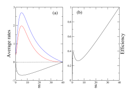
Figure 1: (Color on line) (a) The average rates $\langle\sigma^{m}\rangle$ (black line), $\langle\sigma\rangle$ (red line), and $\langle\imath^{v}\rangle$ (blue line) as a function of the feedback gain $g$. One has $\langle\sigma\rangle=\langle\sigma^{m}\rangle+\langle\imath^{v}\rangle\geq 0$. (b) The most probable efficiency $\bar{\epsilon}=-\langle\sigma^{m}\rangle/\langle\imath^{v}\rangle$ as a function of $g$.

Let us first recall that cooling [$T_{\rm kin}<T$ and thus $\langle\sigma^{m}\rangle=(1/\tau^{v})(T_{\rm kin}-T)<0$] requires $g/\mbox{SNR}<1$, independent of the value of $\tau$ (cf. eq. (20) in HS2014 with the noise variance $\sigma^{2}$ replaced by $\Delta$). This is illustrated in Fig. 1(a) where we plot the average rates as a function of $g$. The most salient features are the extrema in $\langle\sigma^{m}\rangle$ and $\langle\imath^{v}\rangle$. The minimum in $\langle\sigma^{m}\rangle$ occurs at $g=g_{\rm opt}=\sqrt{1+\mbox{SNR}}-1$ HS2014 . Above $g_{\rm opt}$, too much measurement noise is fed back to the system, causing $T_{\rm kin}$ to increase with $g$, a well-known experimental fact PZ2012 . Eventually, for $g/\mbox{SNR}>1$, the system is heated instead of cooled. On the other hand, for $\tau\neq 0$, the maximum in the information flow occurs at $g_{\rm KB}=g_{\rm opt}[1-(\tau/\tau^{v})\sqrt{1+\mbox{SNR}}]<g_{\rm opt}$. The demon then realizes a Kalman-Bucy filter AM2008 (hence the notation $g_{\rm KB}$). In this limit, $\hat{v}_{t}\equiv(\tau/\tau^{v})g_{\rm opt}y_{t}$ represents the best estimate of $v_{t}$ in terms of the mean-squared error ${\cal E}_{t}=\langle(v_{t}-\hat{v}_{t})^{2}\rangle$, given all past measurements HS2014 ; SDNM2014 (recall that (II) describes a non-Markovian control protocol SU2012 ). Interestingly, as shown in HS2014 , $\langle\imath^{v}\rangle$ is then equal to the transfer entropy rate $g_{\rm opt}/2$. We see in Fig. 1(b) that these extrema in $\langle\sigma^{m}\rangle$ and $\langle\imath^{v}\rangle$ induce a local minimum in the information efficiency $\bar{\epsilon}$. This minimum would exactly occur at $g_{\rm opt}$ if $\tau$ were zero (note that $\bar{\epsilon}=1$ for $g/\mbox{SNR}=1$, when the demon does not extract any work.).

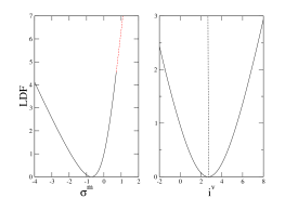
Figure 2: (Color on line) Large deviation functions $E(\sigma^{m})$ (left) and $E(\imath^{v})$ (right) at maximum power ($g=g_{\rm opt}$). The FT symmetry $E(\sigma^{m})-E(-\sigma^{m})=(\frac{2T}{\Delta\kappa}-1)\sigma^{m}$ is obeyed for $|\sigma^{m}|<0.712$ whereas $E(\sigma^{m})$ is linear for $\sigma^{m}>0.712$ (dashed red line). $E(\imath^{v})$ is symmetric around its minimum.

We now fix the gain at its optimal value $g_{\rm opt}$ and investigate the fluctuations. We stress that $g_{\rm opt}$ is close to $g_{\rm KB}$ with our choice of the parameters, so that $\langle\imath^{v}\rangle$ is almost maximal (and the so-called sensory capacity HBS2016 is close to $1$). The large deviation functions $E(\sigma^{m})$ and $E(\imath^{v})$ are plotted in Fig. 2. Notice that $E(\sigma^{m})$ has a linear branch for $\sigma^{m}>0.712$ due to the presence of a pole in the pre-exponential factor. As a result, the steady-state FT (29) does not hold for large values of $\sigma^{m}$ (this, however, corresponds to extremely rare events and depends on the choice of the model parameters). More intriguing is the symmetry exhibited by $E(\imath^{v})$ around its minimum, which we already pointed out. This implies that positive and negative fluctuations of $I^{v}$ around the expectation value are equiprobable. While we have no complete analytic proof nor heuristic argument, we believe this symmetry is a general property of our model even for finite-time fluctuations. This is indeed suggested by numerical simulations as well as by a small-$t$ expansion of the modified generating function $Z_{\imath^{v}}(\lambda,t)e^{\lambda\langle\imath^{v}\rangle t}=\langle e^{-\lambda[I^{v}-\langle I^{v}\rangle]}\rangle$ displaying only even powers of $\lambda$ (see SM). It should be added that perturbative calculations show that the symmetry is lost when there are nonlinearities in the feedback control note1 .

Figure 3: Large deviation function of the efficiency $E(\varepsilon)$ for $g=g_{\rm opt}$. The most and least probable values are $\varepsilon_{\rm most}=\bar{\epsilon}\approx 0.268$ and $\varepsilon_{\rm least}\approx-0.225$.

The LDF for the efficiency $\epsilon$ is obtained from the joint SCGF $\mu_{\sigma^{m},\imath^{v}}(\lambda_{1},\lambda_{2})$ as $E(\epsilon)=-\inf_{\lambda_{1}}\mu_{\sigma^{m},\imath^{v}}(\lambda_{1},\epsilon\lambda_{1})$ and is plotted in Fig. 3. Like in the case of stochastic heat engines VWVE2014 ; GRVG2014 ; PVE2015 ; PCV2015 ; MRDPPR2016 , $E(\epsilon)$ is a non-monotonic function with a minimum at the most probable value $\bar{\epsilon}$ and equal asymptotes for $\epsilon\to\pm\infty$ (the convergence to the asymptotic limit is slow, likely following a power law PVE2015 ; PCV2015 ). We observe that the least probable value of $\epsilon$, corresponding to the maximum of $E(\epsilon)$, is negative. This feature distinguishes the present “information engine” from the stochastic heat engines studied in VWVE2014 ; GRVG2014 ; PVE2015 ; PCV2015 ; MRDPPR2016 .

Having determined the LDFs for information and heat, we now turn to the structure and origin of these fluctuations. We begin by addressing the typical information required to produce a rare fluctuation of heat, or the other way around. In Fig. 4, we plot the most probable value of $\imath^{v}$ (resp. $\sigma^{m}$) for a given rare fluctuation of $\sigma^{m}$ (resp. $\imath^{v}$). These quantities are computed from the derivatives of the joint SCGF $\mu_{\sigma^{m},\imath^{v}}(\lambda_{1},\lambda_{2})$ at $\lambda_{2}=0$ (resp. $\lambda_{1}=0$) (see SM) (note that we restrict our study to the range $\sigma^{m}<0.712$ where fluctuations of the boundary term are irrelevant).

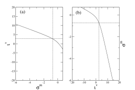
Figure 4: (a) Most probable value of $\imath^{v}$ for a given value of $\sigma^{m}$. (b) Most probable value of $\sigma^{m}$ for a given value of $\imath^{v}$. The dashed lines indicate the typical values $\langle\sigma^{m}\rangle\approx-0.72$ and $\langle\imath^{v}\rangle\approx 2.70$.

As could be expected intuitively, the fluctuations of $\sigma^{m}$ and $\imath^{v}$ are strongly correlated. But a less predictable and remarkable feature is the asymmetry between positive and negative fluctuations: observing a negative fluctuation $\sigma^{m}<\langle\sigma^{m}\rangle$ (resp. a positive fluctuation $\imath^{v}>\langle\imath^{v}\rangle$) for a long time requires a smaller (resp. larger) variation of $\imath^{v}$ (resp. $\sigma^{m}$) than observing $\sigma^{m}>\langle\sigma^{m}\rangle$ (resp. $\imath^{v}<\langle\imath^{v}\rangle$).

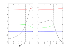
Figure 5: (Color on line) Effective interactions of the auxiliary processes that generate atypical values of $\sigma^{m}$ (left panel) or $\imath^{v}$ (right panel): $\gamma_{\rm eff}$ (black line), $\kappa_{\rm eff}$ (red line), $k_{1}$ (blue line), $k_{2}$ (green line). Vertical dashed lines indicate the typical values of $\sigma^{m}$ and $\imath^{v}$.

Deeper insight into the origin of these fluctuations is offered by studying the two auxiliary (or driven) processes GL2010 ; JS2010 ; CT2013 that generate the constrained ensembles ${\cal P}[{\bf v}_{0}^{t},{\bf y}_{0}^{t}|\Sigma^{m}=\sigma^{m}t]$ or ${\cal P}[{\bf v}_{0}^{t},{\bf y}_{0}^{t}|I^{v}=\imath^{v}t]$ asymptotically. Rare fluctuations then become typical. These auxiliary dynamics are again linear (see SM for details), with modified effective interactions

$$m\dot{v}_{t} =-\gamma_{\rm eff}v_{t}-\kappa_{\rm eff}y_{t}+\xi_{t}$$

$$\tau\dot{y}_{t} =k_{1}y_{t}+k_{2}v_{t}+\eta_{t}\ .$$ (30)

The variations of the coefficients with $\sigma^{m}$ or $\imath^{v}$ are shown in Fig. 5. Again, we observe different behavior for negative and positive fluctuations. The atypical events $\sigma^{m}<\langle\sigma^{m}\rangle$ or $\imath^{v}>\langle\imath^{v}\rangle$ are created essentially by a decrease of the friction coefficient, which even becomes negative ($\kappa_{\rm eff}$ and $k_{2}$ also vary, but slightly, and $k_{1}$ does not change). As a result, the fluctuations of $v_{t}$ are enhanced, as confirmed by Fig. 6, and the effective kinetic temperature increases. This additional uncertainty about $v_{t}$ allows for more information to be gathered, leading to the corresponding increase in $\imath^{v}$ observed in Fig. 3a. In other words, acquiring more information does not necessarily mean that it is effectively used to cool the system.

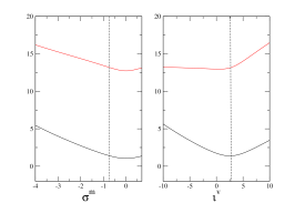
Figure 6: (Color on line) $\langle v^{2}_{t}\rangle$ (black line) and $\langle y^{2}_{t}\rangle$ (red line) conditioned on a given value of $\sigma^{m}$ (left) or $\imath^{v}$ (right).

The case of atypical events $\sigma^{m}>\langle\sigma^{m}\rangle$ or $\imath^{v}<\langle\imath^{v}\rangle$ is not so simple, as both $\gamma_{\rm eff}$ and $k_{2}$ vary significantly. Moreover, $\gamma_{\rm eff}$ is not a monotonic function of $\imath^{v}$. Remarkably, $k_{2}$ becomes very small as $\imath^{v}$ becomes very negative. The demon then does not perform any measurement, and $y_{t}$ just plays the role of additional noise.

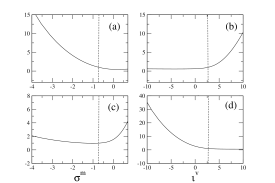
Figure 7: Intensity of the atypical noises as a function of $\sigma^{m}$ or $\imath^{v}$. (a) and (b): $S_{\xi_{\rm atyp}}(\omega=0)/(2\gamma T)$; (c) and (d): $S_{\eta_{\rm atyp}}(\omega=0)/\Delta$. Vertical dashed lines indicate the typical values of $\sigma^{m}$ and $\imath^{v}$.

An alternative approach to understanding the origin of large deviations is to consider the atypical noise realizations that create rare fluctuations and determine whether fluctuations in $\xi_{t}$ or $\eta_{t}$ play the dominant role. To this end, we select an atypical trajectory $({\bf v}_{0}^{t},{\bf y}_{0}^{t})_{\rm atyp}$ produced by the auxiliary processes (III.2.1) for a given value of $\sigma^{m}$ or $\imath^{v}$ and insert it into the original equations of motion (II). This yields two biased noises $\xi_{\rm atyp}$ and $\eta_{\rm atyp}$. Thanks to the linearity of the equations, this calculation can be performed by working in the frequency domain, which yields

$$\xi_{\rm atyp}(\omega) =(\gamma-im\omega)v_{\rm atyp}(\omega)+\kappa\>y_{\rm atyp}(\omega)$$

$$=\frac{\chi_{\rm eff}(\omega)}{k_{1}+i\omega\tau}\Big{[}[(\gamma-im\omega)(k_{1}+i\omega\tau)-\kappa k_{2}]\xi(\omega)$$

$$+[(\gamma-im\omega)\kappa_{\rm eff}-(\gamma_{\rm eff}-im\omega)\kappa]\eta(\omega)\Big{]}$$

$$\eta_{\rm atyp}(\omega) =(1-i\omega\tau)y_{\rm atyp}(\omega)-v_{\rm atyp}(\omega)$$

$$=-\frac{\chi_{\rm eff}(\omega)}{k_{1}+i\omega\tau}\Big{[}[(k_{1}+i\omega\tau)+k_{2}(1-i\omega\tau)]\xi(\omega)$$

$$+[(\gamma_{\rm eff}-im\omega)(1-i\omega\tau)+\kappa_{\rm eff}]\eta(\omega)\Big{]}\ ,$$ (31)

with

$$\chi_{\rm eff}(\omega)=\frac{k_{1}+i\omega\tau}{(\gamma_{\rm eff}-im\omega)(k_{1}+i\omega\tau)-\kappa_{\rm eff}k_{2}}\ .$$ (32)

Therefore, the two noises are correlated and colored, with power spectral densities $S_{\xi_{\rm atyp}}(\omega)=\langle\xi_{\rm atyp}(\omega)\xi_{\rm atyp}(-\omega)\rangle$ and $S_{\eta_{\rm atyp}}(\omega)=\langle\eta_{\rm atyp}(\omega)\eta_{\rm atyp}(-\omega)\rangle$. For simplicity, we here only characterize $\xi_{\rm atyp}$ and $\eta_{\rm atyp}$ by their intensity, that is the zero-frequency part of their power spectrum. The variations of $S_{\xi_{\rm atyp}}(\omega=0)$ and $S_{\xi_{\rm atyp}}(\omega=0)$ (normalized by the intensities of the original white noises) as a function of $\sigma^{m}$ or $\imath^{v}$ are shown in Fig. 7. The overall picture is again very instructive: atypical events $\sigma^{m}<\langle\sigma^{m}\rangle$ or $\imath^{v}>\langle\imath^{v}\rangle$ are mainly due to an atypical history of the thermal noise $\xi_{t}$ whereas atypical events $\sigma^{m}>\langle\sigma^{m}\rangle$ or $\imath^{v}<\langle\imath^{v}\rangle$ are mainly due to an atypical history of the measurement noise $\eta_{t}$.

VI Conclusion

In this Letter, we have studied a Brownian particle model of feedback cooling, as a realization of an autonomous Maxwell’s demon. We have first derived a series of fluctuation theorems for the information flow and the partial entropy production in coupled diffusion processes. We then investigated the fluctuations of information flow and entropy flow, and their correlations, focusing on the long-time limit. By analyzing in detail the effective dynamics and atypical noise realizations that instigate rare fluctuations, we have unraveled the subtle trade-off between noise in the system, noise in the measurement device, and control efficiency. We believe that using the same approach with other models of Maxwell’s demon could significantly improve our understanding of the thermodynamics of information.

Supplemental Material

I Fluctuation relations

I.1 IFT for $\Sigma$

We first derive the IFT for the (partial) entropy production $\Sigma=\Sigma^{v}+I^{v}$. As stated in the main text, this boils down to showing that

$$\Sigma =\ln\frac{{\cal P}[{\bf v}_{0}^{t},{\bf y}_{0}^{t}]}{{\cal P}^{*}[\tilde{\bf v}_{0}^{t},\tilde{\bf y}_{0}^{t}]}\ ,$$ (S1)

where ${\cal P}^{*}[\tilde{\bf v}_{0}^{t},\tilde{\bf y}_{0}^{t}]\equiv{\cal P}^{*}[\tilde{\bf v}_{0}^{t}|\tilde{\bf y}_{0}^{t},\tilde{v}_{0}]{\cal P}^{*}[\tilde{\bf y}_{0}^{t}|\tilde{\bf v}_{0}^{t},\tilde{y}_{0}]p_{t}(v_{t},y_{t})$ is the joint probability density of the time-reversed path $(\tilde{\bf v}_{0}^{t},\tilde{\bf y}_{0}^{t})=(-{\bf v}_{t}^{0},{\bf y}_{t}^{0})$ generated by a modified process, hereafter denoted by the star symbol. The probabilities ${\cal P}[{\bf v}_{0}^{t}|{\bf y}_{0}^{t},v_{0}]$, ${\cal P}[{\bf y}_{0}^{t}|{\bf v}_{0}^{t},y_{0}]$, etc. are expressed in terms of Onsager-Machlup (OM) action functionals.

Following [8], we anticipate that the star dynamics only modifies the equation of motion for $y_{t}$, so that ${\cal P}^{*}[\tilde{\bf v}_{0}^{t},\tilde{\bf y}_{0}^{t}]={\cal P}[\tilde{\bf v}_{0}^{t}|\tilde{\bf y}_{0}^{t},\tilde{v}_{0}]{\cal P}^{*}[\tilde{\bf y}_{0}^{t}|\tilde{\bf v}_{0}^{t},\tilde{y}_{0}]p_{t}(v_{t},y_{t})$. Therefore,

$$\ln\frac{{\cal P}[{\bf v}_{0}^{t},{\bf y}_{0}^{t}]}{{\cal P}^{*}[\tilde{\bf v}_{0}^{t},\tilde{\bf y}_{0}^{t}]}=\Sigma^{m}+\ln\frac{{\cal P}[{\bf y}_{0}^{t}|{\bf v}_{0}^{t},y_{0}]p_{0}(v_{0},y_{0})}{{\cal P}^{*}[\tilde{\bf y}_{0}^{t}|\tilde{\bf v}_{0}^{t},\tilde{y}_{0}]p_{t}(v_{t},y_{t})}\ ,$$ (S2)

where we have used the local detailed balance relation $\ln\big{(}{\cal P}[{\bf v}_{0}^{t}|{\bf y}_{0}^{t},v_{0}]/{\cal P}[\tilde{\bf v}_{0}^{t}|\tilde{\bf y}_{0}^{t},\tilde{v}_{0}]\big{)}=\Sigma^{m}$. Introducing the quantity $\dot{s}_{t}^{v}(v_{t},y_{t})$, we see that eq. (S1) is satisfied if

$$\ln\frac{{\cal P}[{\bf y}_{0}^{t}|{\bf v}_{0}^{t},y_{0}]}{{\cal P}^{*}[\tilde{\bf y}_{0}^{t}|\tilde{\bf v}_{0}^{t},\tilde{y}_{0}]} =\int_{0}^{t}dt^{\prime}\>{\dot{s}}_{t^{\prime}}^{v}(v_{t^{\prime}},y_{t^{\prime}})+\ln\frac{p_{t}(v_{t},y_{t})}{p_{0}(v_{0},y_{0})}$$

$$\equiv-\int_{0}^{t}dt^{\prime}\>{\dot{s}}_{t^{\prime}}^{y}(v_{t^{\prime}},y_{t^{\prime}})$$ (S3)

where ${\dot{s}}_{t}^{y}(v_{t},y_{t})\equiv\frac{d}{dt}s_{t}(v_{t},y_{t})-{\dot{s}}_{t}^{v}(v_{t},y_{t})$ is the time-variation of the stochastic joint entropy $s_{t}(v_{t},y_{t})$ due to $y$’s dynamics. Hence

$${\dot{s}}_{t}^{y}(v_{t},y_{t})=\frac{1}{p_{t}(v_{t},y_{t})}\partial_{y}J^{y}_{t}(v_{t},y_{t})-\dot{y}_{t}\partial_{y}\ln p_{t}(v_{t},y_{t})\ .$$ (S4)

Thus, the derivation of the IFT rests on the construction of a Langevin process that generates trajectories ${\bf y}_{0}^{t}$ with a conditional weight ${\cal P}^{*}[\tilde{\bf y}_{0}^{t}|\tilde{\bf v}_{0}^{t},\tilde{y}_{0}]$ obeying eq. (I.1). As we now show, this process is governed by the equation of motion

$$\tau\dot{y}_{t}=v_{t}+y_{t}+\frac{\Delta}{\tau}\partial_{y}\ln p_{t}(-v_{t},y_{t})+\eta_{t}\ ,$$ (S5)

where $\eta_{t}$ is the same Gaussian white noise as in the original process. Equation (S5) may be viewed as an overdamped Langevin equation with a time-dependent force $F^{*}(v_{t},y_{t},t)=v_{t}+y_{t}+(\Delta/\tau)\partial_{y}\ln p_{t}(-v_{t},y_{t})$ and $\tau^{-1}$ playing the role of a mobility $\mu_{y}$. Hence

$${\cal P}^{*}[\tilde{\bf y}_{0}^{t}|\tilde{\bf v}_{0}^{t},\tilde{y}_{0}] \propto e^{-\frac{1}{2\Delta}\int_{0}^{t}dt^{\prime}\>[\tau\dot{y}_{t^{\prime}}-F^{*}(v_{t^{\prime}},y_{t^{\prime}},t^{\prime})]^{2}-\frac{1}{2\tau}\int_{0}^{t}dt^{\prime}\>\partial_{y}F(v_{t^{\prime}},y_{t^{\prime}},t^{\prime})}$$

$$\propto e^{-\frac{t}{2\tau}}e^{-\frac{1}{2\Delta}\int_{0}^{t}dt^{\prime}\>\big{\{}[\tau\dot{y}_{t^{\prime}}-v_{t^{\prime}}+y_{t^{\prime}}+\frac{\Delta}{\tau}\partial_{y}\ln p_{t^{\prime}}(v_{t^{\prime}},y_{t^{\prime}})]^{2}+(\frac{\Delta}{\tau})^{2}\partial_{y}^{2}\ln p_{t^{\prime}}(v_{t^{\prime}},y_{t^{\prime}})]\big{\}}}\ ,$$ (S6)

where we have changed $t^{\prime}$ into $-t^{\prime}$ in the second line of the equation (we recall that the velocity $v_{t}$ is odd under time reversal but that $y_{t}$ must be treated as an even variable [16]). Comparing with the conditional density associated with the original Langevin equation,

$${\cal P}[{\bf y}_{0}^{t}|{\bf v}_{0}^{t},y_{0}]\propto e^{\frac{t}{2\tau}}e^{-\frac{1}{2\Delta}\int_{0}^{t}dt^{\prime}\>[\tau\dot{y}_{t^{\prime}}+y_{t^{\prime}}-v_{t^{\prime}}]^{2}}\ ,$$ (S7)

we obtain

$$\ln\frac{{\cal P}[{\bf y}_{0}^{t}|{\bf v}_{0}^{t},y_{0}]}{{\cal P}^{*}[\tilde{\bf y}_{0}^{t}|\tilde{\bf v}_{0}^{t},\tilde{y}_{0}]}=\frac{t}{\tau}+\frac{1}{\tau}\int_{0}^{t}dt^{\prime}\>\big{\{}(\tau\dot{y}_{t^{\prime}}+y_{t^{\prime}}-v_{t^{\prime}})\partial_{y}\ln p_{t^{\prime}}(v_{t^{\prime}},y_{t^{\prime}})+\frac{\Delta}{2\tau}\frac{\partial_{y}^{2}p_{t^{\prime}}(v_{t^{\prime}},y_{t^{\prime}})}{p_{t^{\prime}}(v_{t^{\prime}},y_{t^{\prime}})}\big{\}}\ ,$$ (S8)

where we have used the identity $(\partial_{y}\ln f)^{2}+\partial_{y}^{2}\ln f=f^{-1}\partial_{y}^{2}f$. On the other hand, by inserting the expression of the probability current $J_{t}^{y}(v_{t},y_{t})=-\tau^{-1}(y_{t}-v_{t})p(v_{t},y_{t})-\Delta/(2\tau^{2})\partial_{y}p_{t}(v_{t},y_{t})$ into eq. (S4), we find

$$\dot{s}_{t}^{y}(v_{t},y_{t})=-\frac{1}{\tau}-\frac{1}{\tau}(y_{t}-v_{t})\partial_{y}\ln p_{t}(v_{t},y_{t})-\frac{\Delta}{2\tau^{2}}\frac{\partial_{y}^{2}\>p_{t}(v_{t},y_{t})}{p_{t}(v_{t},y_{t})}-\dot{y}_{t}\partial_{y}\ln p_{t}(v_{t},y_{t})\ .$$ (S9)

Therefore eq. (I.1) is satisfied, as announced.

As stated in the main text, the IFT holds for any coupled Langevin processes involving independent noises, for instance the two overdamped Langevin equations (17). Eq. (S8) is then replaced by

$$\ln\frac{{\cal P}[{\bf y}_{0}^{t}|{\bf x}_{0}^{t},y_{0}]}{{\cal P}^{*}[\tilde{\bf y}_{0}^{t}|\tilde{\bf x}_{0}^{t},\tilde{y}_{0}]} =\frac{1}{4T_{y}}\int_{0}^{t}dt^{\prime}\>\Big{[}2\dot{y}_{t^{\prime}}-\mu_{y}[F_{2}(x_{t^{\prime}},y_{t^{\prime}},t^{\prime})-F_{2}^{*}(x_{t^{\prime}},y_{t^{\prime}},t^{\prime})]\Big{]}\Big{[}F_{2}(x_{t^{\prime}},y_{t^{\prime}},t^{\prime})+F_{2}^{*}(x_{t^{\prime}},y_{t^{\prime}},t^{\prime})\Big{]}$$

$$-\frac{\mu_{y}}{2}\int_{0}^{t}dt^{\prime}\>\partial_{y}[F_{2}(x_{t^{\prime}},y_{t^{\prime}},t^{\prime})-F_{2}^{*}(x_{t^{\prime}},y_{t^{\prime}},t^{\prime})]\ ,$$ (S10)

where $F_{2}^{*}(x,y,t)$ is the force acting on $y_{t}$ in the modified dynamics. Then, by choosing

$$F_{2}^{*}(x,y,t)=-F_{2}(x_{t},y_{t},t)+2T_{y}\partial_{y}\ln p_{t}(x_{t},y_{t})\ ,$$ (S11)

the r.h.s. of eq. (I.1) identifies with $\int_{0}^{t}dt^{\prime}\>\dot{s}_{t}^{y}(x_{t^{\prime}},y_{t^{\prime}})$, with $\dot{s}_{t}^{y}(v_{t},y_{t})$ defined by eq. (S4). We leave the demonstration as an exercise for the reader.

I.2 IFT for $I^{v}$

The IFT for the integrated information flow [eq. (21) in the main text] is obtained by modifying also the dynamics of $v_{t}$ and changing $\gamma$ into $-\gamma$ while keeping the variance of $\xi_{t}$ fixed (this modified process is denoted by the hat symbol hereafter). As shown in [28], this leads to

$$\frac{{\cal P}[{\bf v}_{0}^{t}|{\bf y}_{0}^{t},v_{0}]}{\hat{\cal P}[{\bf v}_{0}^{t}|{\bf y}_{0}^{t},v_{0}]}=e^{\frac{\gamma}{m}t}e^{\Sigma^{m}}\ .$$ (S12)

By replacing the trajectories by their time-reversed images, this relation can be rewritten as

$$\Sigma^{m}=\frac{\gamma}{m}t+\ln\frac{\hat{\cal P}[\tilde{\bf v}_{0}^{t}|\tilde{\bf y}_{0}^{t},\tilde{v}_{0}]}{{\cal P}[\tilde{\bf v}_{0}^{t}|\tilde{\bf y}_{0}^{t},\tilde{v}_{0}]}\ .$$ (S13)

Therefore, using eq. (S1), we have

$$\Sigma-\Sigma^{m} =-\frac{\gamma}{m}t+\ln\frac{{\cal P}[{\bf v}_{0}^{t},{\bf y}_{0}^{t}]}{{\cal P}^{*}[\tilde{\bf v}_{0}^{t},\tilde{\bf y}_{0}^{t}]}-\ln\frac{\hat{\cal P}[\tilde{\bf v}_{0}^{t}|\tilde{\bf y}_{0}^{t},\tilde{v}_{0}]}{{\cal P}[\tilde{\bf v}_{0}^{t}|\tilde{\bf y}_{0}^{t},\tilde{v}_{0}]}$$

$$=-\frac{\gamma}{m}t+\ln\frac{{\cal P}[{\bf v}_{0}^{t},{\bf y}_{0}^{t}]}{{\cal P}[\tilde{\bf v}_{0}^{t}|\tilde{\bf y}_{0}^{t},\tilde{v}_{0}]{\cal P}^{*}[\tilde{\bf y}_{0}^{t}|\tilde{\bf v}_{0}^{t},\tilde{y}_{0}]p_{t}(v_{t},y_{t})}-\ln\frac{\hat{\cal P}[\tilde{\bf v}_{0}^{t}|\tilde{\bf y}_{0}^{t},\tilde{v}_{0}]}{{\cal P}[\tilde{\bf v}_{0}^{t}|\tilde{\bf y}_{0}^{t},\tilde{v}_{0}]}$$

$$=-\frac{\gamma}{m}t+\ln\frac{{\cal P}[{\bf v}_{0}^{t},{\bf y}_{0}^{t}]}{\hat{\cal P}^{*}[\tilde{\bf v}_{0}^{t},\tilde{\bf y}_{0}^{t}]}\ ,$$ (S14)

where $\hat{\cal P}^{*}[\tilde{\bf v}_{0}^{t},\tilde{\bf y}_{0}^{t}]\equiv\hat{\cal P}[\tilde{\bf v}_{0}^{t}|\tilde{\bf y}_{0}^{t},\tilde{v}_{0}]{\cal P}^{*}[\tilde{\bf y}_{0}^{t}|\tilde{\bf v}_{0}^{t},\tilde{y}_{0}]p_{t}(v_{t},y_{t})$ is the joint probability density of the backward path generated by the modified “hat-star” processs (i.e., the “hat” dynamics for $v_{t}$ and the “star” dynamics for $y_{t}$). Since $\Sigma-\Sigma^{m}=I^{v}-\ln p_{t}(v_{t})/p_{0}(v_{0})$ (cf. eqs. (8) and (9) in the main text), we finally obtain

$$\frac{p_{t}(v_{t})}{p_{0}(v_{0})}e^{-I^{v}} =e^{\frac{\gamma}{m}t}\frac{\hat{\cal P}^{*}[\tilde{\bf v}_{0}^{t},\tilde{\bf y}_{0}^{t}]}{{\cal P}[{\bf v}_{0}^{t},{\bf y}_{0}^{t}]}\ ,$$ (S15)

which leads to the IFT for the information flow by integration over the ensemble of paths generated by the original process. Note that this IFT is less general than the one for $\Sigma$ since the force acting on the state variable of the first subsystem must be linear. This is true for the model under study since this force is just the viscous force $-\gamma v_{t}$. For the coupled overdamped Langevin processes described by eqs. (17), one must have $F_{1}(x,y,t)=-kx_{t}+F(y_{t},t)$. Then $(\gamma/m)t$ is replaced by $(\mu_{x}k)t$ in eqs. (S12)-(S15) (see [28] for a more general discussion).

II Scaled cumulant generating functions

In this section we derive eqs. (27) in the main text, and we discuss the domain of validity of these expressions. We also give the expressions of $\mu_{\sigma}(\lambda)$ and of the joint SCGF $\mu_{\sigma^{m},\imath^{v}}(\lambda_{1},\lambda_{2})$. These results are obtained by imposing periodic boundary conditions on the trajectories and expanding $v_{t}$ and $y_{t}$ in discrete Fourier series,

$$v(t) =\sum_{n=-\infty}^{\infty}v_{n}e^{-i\omega_{n}t}$$

$$y(t) =\sum_{n=-\infty}^{\infty}y_{n}e^{-i\omega_{n}t}\ ,$$ (S16)

with inverse transforms

$$v_{n} =\frac{1}{t}\int_{0}^{t}ds\>v(s)e^{i\omega_{n}s}$$

$$y_{n} =\frac{1}{t}\int_{0}^{t}ds\>y(s)e^{i\omega_{n}s}\ ,$$ (S17)

where $\omega_{n}=2\pi n/t$ and $v_{n}\equiv v(\omega_{n})$, $y_{n}\equiv y(\omega_{n})$. The coupled Langevin equations in the frequency domain are then

$$(\gamma-im\omega_{n})v_{n} =-\kappa y_{n}+\xi_{n}$$

$$(1-i\omega_{n}\tau)y_{n} =v_{n}+\eta_{n}\ ,$$ (S18)

with $\langle\xi_{n}\xi_{n^{\prime}}\rangle=(2\gamma T/t)\delta_{n,-n^{\prime}}$, $\langle\eta_{n}\eta_{n^{\prime}}\rangle=(\Delta/t)\delta_{n,-n^{\prime}}$, and $\langle\xi_{n}\eta_{n^{\prime}}\rangle=0$. This leads to

$$v_{n} =\chi_{n}[\xi_{n}-\frac{\kappa}{1-i\omega_{n}\tau}\eta_{n}]$$

$$y_{n} =\frac{\chi_{n}}{1-i\omega_{n}\tau}[\xi_{n}+(\gamma-im\omega_{n})\eta_{n}]$$ (S19)

where

$$\chi_{n}\equiv\chi(\omega_{n})=\frac{1-i\omega_{n}\tau}{\kappa+\gamma-i(m+\gamma\tau)\omega_{n}-m\omega_{n}^{2}\tau}\ .$$ (S20)

II.1 SCGFs for single observables

For brevity, we will only detail the calculation of $\mu_{\imath^{v}}(\lambda)$. In the stationary state, $I^{v}$ is given by eq. (23) in the main text. We recall that $\alpha_{11},\alpha_{22}$ and $\alpha_{12}=\alpha_{21}$ are the entries of ${\bf C}^{-1}$, the inverse of the covariance matrix whose expression is given in Appendix D of [16]. In terms of the Fourier coefficients $v_{n}$ and $y_{n}$, the rate $\imath^{v}\equiv I^{v}/t$ reads

$$\imath^{v} =-A_{1}+\sum_{n=-\infty}^{\infty}[\alpha_{11}A_{1}v_{n}v_{-n}+A_{2}y_{n}y_{-n}+(A_{3}-i\omega_{n}\alpha_{12})v_{n}y_{-n}]+b.t.$$ (S21)

where $b.t.$ is a temporal boundary term that is neglected hereafter (see the discussion below). Inserting eqs. (II) then yields

$$\imath^{v} \sim-A_{1}+\sum_{n=-\infty}^{\infty}\frac{|\chi_{n}|^{2}}{1+\omega_{n}^{2}\tau^{2}}\Big{\{}[\alpha_{11}A_{1}(1+\omega_{n}^{2}\tau^{2})+A_{2}+(A_{3}-i\omega_{n}\alpha_{12})(1-i\omega_{n}\tau)]|\xi_{n}|^{2}$$

$$+[\kappa^{2}\alpha_{11}A_{1}+(\gamma^{2}+m^{2}\omega_{n}^{2})A_{2}-\kappa(A_{3}-i\omega_{n}\alpha_{12})(\gamma+im\omega_{n})]|\eta_{n}|^{2}$$

$$+[-\kappa\alpha_{11}A_{1}(1-i\omega_{n}\tau)+(\gamma+im\omega_{n})A_{2}+(A_{3}-i\omega_{n}\alpha_{12})(\gamma+im\omega_{n})(1-i\omega_{n}\tau)]\xi_{n}\eta_{-n}$$

$$+[-\kappa\alpha_{11}A_{1}(1+i\omega_{n}\tau)+(\gamma-im\omega_{n})A_{2}-\kappa(A_{3}-i\omega_{n}\alpha_{12})]\xi_{-n}\eta_{n}\Big{\}}\ ,$$ (S22)

which is rewritten in a compact form as

$$\imath^{v} \sim-A_{1}+\sum_{n=1}^{\infty}\zeta_{n}^{T}{\bf L}_{n,\imath^{v}}\zeta^{*}_{n}\ ,$$ (S23)

where $\zeta_{n}=(\xi_{n},\eta_{n})^{T}$, the symbol $*$ denotes the complex conjugate (with $\xi^{*}_{n}=\xi_{-n},\eta^{*}_{n}=\eta_{-n}$), and ${\bf L}_{n,\imath^{v}}$ is a $2\times 2$ Hermitian matrix with entries

$$L_{11,\imath^{v}}(\omega_{n}) =\frac{2|\chi_{n}|^{2}}{1+\omega_{n}^{2}\tau^{2}}[\alpha_{11}A_{1}(1+\omega_{n}^{2}\tau^{2})+A_{2}+A_{3}-\omega_{n}^{2}\tau\alpha_{12}]$$

$$L_{12,\imath^{v}}(\omega_{n}) =L^{*}_{21}(\omega_{n})=\frac{|\chi_{n}|^{2}}{1+\omega_{n}^{2}\tau^{2}}\Big{[}-2\kappa\alpha_{11}A_{1}(1-i\omega_{n}\tau)+2(\gamma+im\omega_{n})A_{2}+A_{3}[(\gamma+im\omega_{n})(1-i\omega_{n}\tau)-\kappa]$$

$$-i\omega_{n}\alpha_{12}[(\gamma+im\omega_{n})(1-i\omega_{n}\tau)+\kappa]\Big{]}$$

$$L_{22,\imath^{v}}(\omega_{n}) =\frac{2|\chi_{n}|^{2}}{1+\omega_{n}^{2}\tau^{2}}[\kappa^{2}\alpha_{11}A_{1}+(\gamma^{2}+m^{2}\omega_{n}^{2})A_{2}-\kappa(A_{3}\gamma+m\omega_{n}^{2}\alpha_{12})]\ .$$ (S24)

This leads to

$$\langle e^{-\lambda I^{v}}\rangle \sim e^{\lambda A_{1}t}\prod_{n=1}^{\infty}\int d\zeta_{n}\>P(\zeta_{n})e^{-\lambda t\>\zeta_{n}^{T}{\bf L}_{n,\imath^{v}}\zeta^{*}_{n}}\ ,$$ (S25)

where

$$P(\zeta_{n})=\frac{1}{\pi^{2}\mbox{det}{\bf D}}e^{-\zeta_{n}{\bf D}^{-1}\zeta_{n}^{*}}$$ (S26)

and

$${\bf D}=\frac{1}{t}\left(\begin{array}[]{cccc}2\gamma T&0\\ 0&\Delta&\end{array}\right)\ .$$

The Gaussian integration over $\zeta_{n}$ then gives

$$\int d\zeta_{n}\>P(\zeta_{n})e^{-\lambda t\>\zeta_{n}^{T}{\bf L}_{n,\imath^{v}}\zeta^{*}_{n}}=\mbox{det}[{\bf I}+\lambda t{\bf D}{\bf L}_{n,\imath^{v}}]^{-1}\ .$$ (S27)

In the long-time limit, the summation over $n$ can be replaced by an integral over $\omega$, and we finally obtain

$$\mu_{\imath^{v}}(\lambda) =\frac{\gamma}{m}(1-T\frac{\alpha_{11}}{m})\lambda-\int_{0}^{\infty}\frac{d\omega}{2\pi}\ln[1-F_{\imath^{v},\lambda}(\omega)]\ ,$$ (S28)

with

$$F_{\imath^{v},\lambda}(\omega)=-2\gamma T\Delta\lambda^{2}[L_{11,\imath^{v}}(\omega)L_{22,\imath^{v}}(\omega)-L_{12,\imath^{v}}(\omega)L_{21,\imath^{v}}(\omega)]\ ,$$ (S29)

which leads to eq. (27b) in the main text.

The calculation of $\mu_{\sigma^{m}}(\lambda)$ is quite similar but somewhat simpler since $\Sigma^{m}=-(\kappa/T)\int_{0}^{t}dt^{\prime}\>v_{t^{\prime}}y_{t^{\prime}}\sim-(\kappa/T)\sum_{n}v_{n}y_{n}$. The entries of the corresponding matrix ${\bf L}_{n,\sigma^{m}}$ are then given by

$$L_{11,\sigma^{m}}(\omega_{n}) =-\frac{2\kappa}{T}\frac{|\chi_{n}|^{2}}{1+\omega_{n}^{2}\tau^{2}}$$

$$L_{12,\sigma^{m}}(\omega_{n}) =L^{*}_{21}(\omega_{n})=-\frac{\kappa}{T}\frac{|\chi_{n}|^{2}}{1+\omega_{n}^{2}\tau^{2}}[(\gamma+im\omega_{n})(1-i\omega_{n}\tau)-\kappa]$$

$$L_{22,\sigma^{m}}(\omega_{n}) =\frac{2\kappa^{2}\gamma}{T}\frac{|\chi_{n}|^{2}}{1+\omega_{n}^{2}\tau^{2}}\ ,$$ (S30)

so that

$$\mu_{\sigma^{m}}(\lambda) =-\int_{0}^{\infty}\frac{d\omega}{2\pi}\ln[1-F_{\sigma^{m},\lambda}(\omega)]\ ,$$ (S31)

with

$$F_{\sigma^{m},\lambda}(\omega)=-\lambda[2\gamma TL_{11,\sigma^{m}}(\omega)+\Delta L_{22,\sigma^{m}}(\omega)]-2\gamma T\Delta\lambda^{2}[L_{11,\sigma^{m}}(\omega)L_{22,\sigma^{m}}(\omega)-L_{12,\sigma^{m}}(\omega)L_{21,\sigma^{m}}(\omega)]\ ,$$ (S32)

which leads to eq. (27a) in the main text. The main difference with $F_{\imath^{v},\lambda}(\omega)$ is that the term linear in $\lambda$ does not vanish so that $F_{\sigma^{m},\lambda}(\omega)$ is not an even function of $\lambda$.

Finally, the expression of $\mu_{\sigma}(\lambda)$ is obtained by exploiting the fact that $\Sigma\sim\Sigma^{m}+I^{v}$ as $t\to\infty$. Hence

$$\mu_{\sigma}(\lambda) =\frac{\gamma}{m}(1-T\frac{\alpha_{11}}{m})\lambda-\int_{0}^{\infty}\frac{d\omega}{2\pi}\ln[1-F_{\sigma,\lambda}(\omega)]\ ,$$ (S33)

with

$$F_{\sigma,\lambda}(\omega)=-\lambda[2\gamma T(L_{11,\sigma}(\omega)+\Delta L_{22,\sigma}(\omega)]-2\gamma T\Delta\lambda^{2}[L_{11,\sigma}(\omega)L_{22,\sigma}(\omega)-L_{12,\sigma}(\omega)L_{21,\sigma}(\omega)]$$ (S34)

and $L_{ij,\sigma}=L_{ij,\sigma^{m}}+L_{ij,\imath^{v}}$.

Note that the SCGFs are real quantities in an open domain $(\lambda_{-},\lambda_{+})$ (different for each function) in which the argument of the logarithm stays positive for all values of $\omega$. For instance, with the choice $\tau/\tau^{v}=0.01,\ \mbox{SNR}=40,\ g=g_{\rm opt}\approx 5.403$ for the model parameters, we find that $\mu_{\imath^{v}}(\lambda)$, $\mu_{\sigma^{m}}(\lambda)$, and $\mu_{\sigma}(\lambda)$ are defined in the intervals $-1.004<\lambda<1.004$, $-8.130<\lambda<1.727$, and $-1.931<\lambda<1.027$, respectively. The slopes of the SCGFs diverge at the boundaries, which implies that the corresponding Legendre transforms are asymptotically linear [29]. However, this is no longer true if the pre-exponential factors (see eq. (25) in the main text and eq. (S44) below) have pole singularities inside the domain of definition. These singularities result from rare but large fluctuations of the boundary terms neglected in the preceding calculation, and the leading contribution to the LDF then comes from the singularity (whose position fixes the slope of the LDF). For instance, $g_{\sigma^{m}}(\lambda)$ diverges for $\lambda=\lambda_{0}\approx-6.39$, so that $E(\sigma^{m})\approx 0.038+6.39\sigma^{m}$ for $\sigma^{m}>-\mu^{\prime}_{\sigma^{m}}(\lambda_{0})\approx 0.712$ (see Fig. 2 of the main text).

II.2 Joint SCGFs

The same method based on discrete Fourier transforms can be used to compute joint SCGFs such as $\mu_{\sigma^{m},\imath^{v}}(\lambda_{1},\lambda_{2})\equiv\lim_{t\to\infty}(1/t)\ln\langle e^{-\lambda_{1}\Sigma^{m}-\lambda_{2}I^{v}}\rangle$. Moreover, since $\Sigma\sim\Sigma^{m}+I^{v}$ in the long-time limit, the three functions $\mu_{\sigma^{m},\imath^{v}}(\lambda_{1},\lambda_{2}),\mu_{\sigma^{m},\sigma}(\lambda_{1},\lambda_{2}),\mu_{\sigma,\imath^{v}}(\lambda_{1},\lambda_{2})$ are not independent. Specifically, $\mu_{\sigma,\imath^{v}}(\lambda_{1},\lambda_{2})=\mu_{\sigma^{m},\imath^{v}}(\lambda_{1},\lambda_{1}+\lambda_{2})$ and $\mu_{\sigma^{m},\sigma}(\lambda_{1},\lambda_{2})=\mu_{\sigma^{m},\imath^{v}}(\lambda_{1}+\lambda_{2},\lambda_{2})$, with

$$\mu_{\sigma^{m},\imath^{v}}(\lambda_{1},\lambda_{2})=\frac{\gamma}{m}(1-T\frac{\alpha_{11}}{m})\lambda_{2}-\frac{1}{2}\int_{-\infty}^{\infty}\frac{d\omega}{2\pi}\>\ln[1-F_{\sigma^{m},\imath^{v},\lambda_{1},\lambda_{2}}(\omega)]$$ (S35)

and

$$F_{\sigma^{m},\imath^{v},\lambda_{1},\lambda_{2}}(\omega) =-2\gamma T[\lambda_{1}L_{11,\sigma^{m}}(\omega)+\lambda_{2}L_{11,\imath^{v}}(\omega)]-\Delta[\lambda_{1}L_{22,\sigma^{m}}(\omega)+\lambda_{2}L_{22,\imath^{v}}(\omega)]$$

$$-2\gamma T\Delta\Big{\{}[\lambda_{1}L_{11,\sigma^{m}}(\omega)+\lambda_{2}L_{11,\imath^{v}}(\omega)][\lambda_{1}L_{22,\sigma^{m}}(\omega)+\lambda_{2}L_{22,\imath^{v}}(\omega)]$$

$$-[\lambda_{1}L_{12,\sigma^{m}}(\omega)+\lambda_{2}L_{12,\imath^{v}}(\omega)][\lambda_{1}L_{12,\sigma^{m}}^{*}(\omega)+\lambda_{2}L_{12,\imath^{v}}^{*}(\omega)]\Big{\}}\ .$$ (S36)

One can readily check that $\mu_{\sigma^{m}}(\lambda)=\mu_{\sigma^{m},\imath^{v}}(\lambda,0)$, $\mu_{\sigma}(\lambda)=\mu_{\sigma^{m},\imath^{v}}(0,\lambda)$, and $\mu_{\sigma}(\lambda)=\mu_{\sigma^{m},\imath^{v}}(\lambda,\lambda)$.

III Tilted and auxiliary processes

In this section, we construct the so-called auxiliary (or driven) processes [24-26] that describe how large fluctuations of $\Sigma^{m}$, $I^{v}$, or $\Sigma$ are created in the long-time limit. For each of these observables, we first determine the so-called tilted generator and compute the dominant eigenvalue and the associated left and right eigenfunctions (the dominant eigenvalue identifies with the SCGF already obtained in section II.1, but the knowledge of the eigenfunctions allows us to compute the pre-exponential factors). We then determine the biased forces or biased noises that make a large deviation of the observable typical.

For brevity, we mostly focus on large deviations of $I^{v}$. We also closely follow the analysis and notations of [26].

III.1 Spectral elements

III.1.1 Tilted generators

From the definition of $I^{v}$ [eqs. (7) and (8) in the main text], we note that this quantity belongs to the general class of trajectory observables of the form [26]

$$I^{v}=\int_{0}^{t}f_{\imath^{v}}({\bf X}_{t})dt^{\prime}+\int_{0}^{t}{\bf g}_{\imath^{v}}({\bf X}_{t^{\prime}})\circ d{\bf X}_{t^{\prime}}\ ,$$ (S37)

where ${\bf X}_{t}=(v_{t},y_{t})$, $f_{\imath^{v}}(v,y)=\partial_{v}J^{v}(v,y)/p(v,y)$ (since $\partial_{v}J(v)=0$ in the stationary state), and ${\bf g}_{\imath^{v}}(v,y)$ is a two-dimensional vector function with components $(-\partial_{v}\ln p(y|v),0)$. We then introduce the non-conservative process associated with the exponentially tilted trajectory ensemble

$${\cal P}_{\imath^{v},\lambda}[{\bf v}_{0}^{t},{\bf y}_{0}^{t}]\equiv\frac{e^{-\lambda I^{v}}{\cal P}[{\bf v}_{0}^{t},{\bf y}_{0}^{t}]}{\langle e^{-\lambda I^{v}}\rangle}$$ (S38)

that becomes equivalent in the limit $t\to\infty$ to the ensemble of trajectories conditioned on a particular value of $\imath^{v}$ (the equivalence holds because the LDF $E(\imath^{v})$ is convex, and the value of $\lambda$ achieving the equivalence is then given by $\lambda=-E^{\prime}(\imath^{v})$). The corresponding tilted generator is given by [26]

$${\cal L}_{\imath^{v}\lambda}={\bf F}(\nabla-\lambda{\bf g}_{\imath^{v}})+(\nabla-\lambda{\bf g}_{\imath^{v}})\frac{{\bf D}^{\prime}}{2}(\nabla-\lambda{\bf g}_{\imath^{v}})-\lambda f_{\imath^{v}}\ ,$$ (S39)

where ${\bf F}$ is the two-dimensional drift of the original process with components $(-(\gamma v+\kappa y)/m,(v-y)/\tau)$ and the noise covariance matrix ${\bf D}^{\prime}$ is here defined as

$${\bf D}^{\prime}=\left(\begin{array}[]{cccc}\frac{2\gamma T}{m^{2}}&0\\ 0&\frac{\Delta}{\tau^{2}}&\end{array}\right)\ .$$

The generating function ${\cal Z}_{\imath^{v},\lambda}(v,y,t)=\langle e^{-\lambda I^{v}}\delta(v-v_{t})\delta(y-y_{t})\rangle$ (where the average is taken over all trajectories of duration $t$ ending at $(v,y)$ with initial state $(v_{0},y_{0})$ drawn from the stationary pdf $p(v_{0},y_{0})$) evolves according to

$$\partial_{t}Z_{\imath^{v},\lambda}(v,y,t)={\cal L}_{\imath^{v},\lambda}^{{\dagger}}Z_{\imath^{v},\lambda}(v,y,t)\ ,$$ (S40)

where ${\cal L}_{\imath^{v},\lambda}^{{\dagger}}$ is the dual of ${\cal L}_{\imath^{v},\lambda}$. Namely,

$${\cal L}_{\imath^{v},\lambda}^{{\dagger}} =\frac{\gamma T}{m^{2}}\frac{\partial^{2}}{\partial v^{2}}+\frac{\Delta}{2\tau^{2}}\frac{\partial^{2}}{\partial y^{2}}+\frac{1}{m}\left[\gamma v+\kappa y-2\frac{\lambda\gamma T}{m}\partial_{v}\ln p(y|v)\right]\partial_{v}+\frac{y-v}{\tau}\partial_{y}$$

$$+\frac{\lambda}{m}\Big{[}\gamma+(\gamma v+\kappa y)\partial_{v}\ln p(v)\Big{]}+\frac{\lambda\gamma T}{m^{2}}\Big{[}(\lambda+1)(\partial_{v}\ln p(y|v))^{2}+2\partial_{v}\ln p(y|v)\partial_{v}\ln p(v)$$

$$+(\partial_{v}\ln p(v))^{2}+\frac{\partial^{2}}{\partial v^{2}}\ln p(v)\Big{]}+\frac{\gamma}{m}+\frac{1}{\tau}\ ,$$ (S41)

with $\partial_{v}\ln p(y|v)=-(\alpha_{11}-c_{11}^{-1})v-\alpha_{12}y$ and $\partial_{v}\ln p(v)=-c_{11}^{-1}v$ (we recall that $c_{ij}$ and $\alpha_{ij}$ are the entries of the covariance matrix and its inverse, respectively).

In order to determine the asymptotic behavior of $Z_{\imath^{v},\lambda}(v,y,t)$, we do not need to solve the spectral problem for ${\cal L}_{\imath^{v},\lambda}$ and ${\cal L}^{{\dagger}}_{\imath^{v},\lambda}$ in full generality but only to compute the dominant eigenvalue $\mu_{\imath^{v}}(\lambda)$ and the associated right and left eigenfunctions, solutions of the equations

$${\cal L}_{\imath^{v},\lambda}\,r_{\imath^{v},\lambda}(v,y)=\mu_{\imath^{v}}(\lambda)\,r_{\imath^{v},\lambda}(v,y)$$

$${\cal L}_{\imath^{v},\lambda}^{{\dagger}}\,l_{\imath^{v},\lambda}(v,y)=\mu_{\imath^{v}}(\lambda)\,l_{\imath^{v},\lambda}(v,y)\ ,$$ (S42)

with normalization conditions $\int dv\>dy\>l_{\imath^{v},\lambda}(v,y)=1$ and $\int dv\>dy\>r_{\imath^{v},\lambda}(v,y)l_{\imath^{v},\lambda}(v,y)=1$. From eq. (III.1.1) and the corresponding expression of ${\cal L}_{\imath^{v}\lambda}$, we find that the bivariate Gaussian functions $r_{\imath^{v},\lambda}(v,y)=e^{-(1/2)[A_{\imath^{v}}(\lambda)v^{2}+B_{\imath^{v}}(\lambda)y^{2}+2C_{\imath^{v}}(\lambda)yv]}$ and $l_{\imath^{v},\lambda}(v,y)=e^{-(1/2)[A_{\imath^{v}}^{{\dagger}}(\lambda)v^{2}+B_{\imath^{v}}^{{\dagger}}(\lambda)y^{2}+2C_{\imath^{v}}^{{\dagger}}(\lambda)yv]}$ are solutions (not yet normalized) of these equations, with the coefficients $A_{\imath^{v}}(\lambda),A_{\imath^{v}}^{{\dagger}}(\lambda)$, etc. obeying complicated algebraic equations. $\mu_{\imath^{v}}(\lambda)$ is eventually obtained as the solution of an algebraic equation of degree $6$, and the proper root is selected by imposing numerical agreement with eq. (S28). Then, assuming the existence of a gap between $\mu_{\imath^{v}}$ and the first sub-dominant eigenvalue, $Z_{\imath^{v},\lambda}(v,y,t)$ takes the asymptotic form [26]

$$Z_{\imath^{v},\lambda}(v,y,t)\sim e^{\mu_{\imath^{v}}(\lambda)t}\int dv_{0}dy_{0}\>p(v_{0},y_{0})r_{\imath^{v},\lambda}(v_{0},y_{0})\>l_{\imath^{v},\lambda}(v,y)\ ,$$ (S43)

so that $Z_{\imath^{v}}(\lambda,t)=\int dv\>dy\>Z_{\imath^{v},\lambda}(v,y,t)\sim g_{\imath^{v}}(\lambda)e^{\mu_{\imath^{v}}(\lambda)t}$ with

$$g_{\imath^{v}}(\lambda)=\int dv_{0}dy_{0}\>p(v_{0},y_{0})r_{\imath^{v},\lambda}(v_{0},y_{0})\ .$$ (S44)

Depending on the model parameters (e.g. the feedback gain), the above integral may diverge for certain values of $\lambda$, signaling that the fluctuations of the temporal boundary terms must not be neglected, as discussed at the end of section B.1.

Similar calculations are performed for $\Sigma^{m}$ and $\Sigma$. For completeness, we report the corresponding expressions of the tilted dual generators ${\cal L}_{\sigma^{m},\lambda}^{{\dagger}}$ and ${\cal L}_{\sigma,\lambda}^{{\dagger}}$:

$${\cal L}_{\sigma^{m},\lambda}^{{\dagger}} =\frac{\gamma T}{m^{2}}\frac{\partial^{2}}{\partial v^{2}}+\frac{\Delta}{2\tau^{2}}\frac{\partial^{2}}{\partial y^{2}}+\frac{1}{m}\left[(1-2\lambda)\gamma v+\kappa y\right]\partial_{v}+\frac{y-v}{\tau}\partial_{y}$$

$$+\lambda\left[(\lambda-1)\gamma\frac{v^{2}}{T}-\frac{\gamma}{m}\right]+\frac{\gamma}{m}+\frac{1}{\tau}\ ,$$ (S45)

and

$${\cal L}_{\sigma,\lambda}^{{\dagger}} =\frac{\gamma T}{m^{2}}\frac{\partial^{2}}{\partial v^{2}}+\frac{\Delta}{2\tau^{2}}\frac{\partial^{2}}{\partial y^{2}}+\frac{1}{m}\left[(1-2\lambda)\gamma v+\kappa y-2\frac{\lambda\gamma T}{m}\partial_{v}\ln p(v,y)\right]\partial_{v}+\frac{y-v}{\tau}\partial_{y}$$

$$+\lambda\left[\gamma v[(\lambda-1)\frac{v}{T}+\frac{2\lambda}{m}\partial_{v}\ln p(v,y)]+(\lambda+1)\frac{\gamma T}{m^{2}}(\partial_{v}\ln p(v,y))^{2}\right]+\frac{\gamma}{m}+\frac{1}{\tau}\ .$$ (S46)

Note that ${\cal L}_{\sigma^{m},\lambda=1}^{{\dagger}}-{\cal L}_{\sigma^{m},\lambda=0}^{{\dagger}}=-2(\gamma/m)v\partial_{v}-(\gamma/m)$ so that $\partial_{t}Z_{\sigma^{m}}(1,t)=(\gamma/m)Z_{\sigma^{m}}(1,t)$ by integration over $v$ and $y$, in agreement with the IFT $Z_{\sigma^{m}}(1,t)=\langle e^{-\Sigma^{m}}\rangle=e^{(\gamma/m)t}$. Likewise, ${\cal L}_{\sigma,\lambda=1}^{{\dagger}}-{\cal L}_{\sigma,\lambda=0}^{{\dagger}}=2(\gamma/m)v+(T/m)\partial_{v}\ln p(v,y)][\partial_{v}\ln p(v,y)-\partial_{v}]$ so that $p(v,y)$ is an eigenfunction of ${\cal L}_{\sigma,\lambda=1}^{{\dagger}}$ associated with the eigenvalue $0$, in agreement with the IFT $\langle e^{-\Sigma}\rangle=1$. However, we stress that the two IFTs for $\Sigma^{m}$ and $\Sigma$ are valid at any time, and not only asymptotically.

III.1.2 Small-$t$ expansion of $Z_{\imath^{v}}(\lambda,t)$

In order to investigate whether the symmetry of the SCGF $\mu_{\imath^{v}}(\lambda)$ [eq. (S28) above] reflects a more general symmetry of the pdf for the information flow, we introduce the modified function $\tilde{Z}_{\imath^{v},\lambda}(v,y,t)=Z_{\imath^{v},\lambda}(v,y,t)e^{\lambda\langle\imath^{v}\rangle t}$ which evolves according to

$$\partial_{t}\tilde{Z}_{\imath^{v},\lambda}(v,y,t)=\tilde{\cal L}_{\imath^{v},\lambda}^{\dagger}\tilde{Z}_{\imath^{v},\lambda}(v,y,t)\ ,$$ (S47)

with $\tilde{\cal L}_{\imath^{v},\lambda}^{\dagger}={\cal L}_{\imath^{v},\lambda}^{\dagger}+\lambda\langle\imath^{v}\rangle$. The solution can be formally expanded in powers of $t$ as

$$\tilde{Z}_{\imath^{v},\lambda}(v,y,t)=p(v,y)+\sum_{n=1}^{\infty}\frac{1}{n!}\tilde{Z}_{\imath^{v},\lambda}^{(n)}(v,y)t^{n}$$ (S48)

with $\tilde{Z}_{\imath^{v},\lambda}^{(n)}(v,y)=(\tilde{\cal L}_{\imath^{v},\lambda}^{\dagger})^{n}p(v,y)$. For brevity, we here only report the expression of the term proportional to $t$,

$$\tilde{Z}_{\imath^{v},\lambda}^{(1)}(v,y)=p(v,y)[f_{0}(v,y)+f_{1}(v,y)\lambda+f_{2}(v,y)\lambda^{2}]\ ,$$ (S49)

with

$$f_{0}(v,y) =\frac{1}{2\tau^{2}m^{2}(c_{11}c_{22}-c_{12}^{2})^{2}}\Big{[}[2\gamma T\tau^{2}c_{22}^{2}+\Delta m^{2}c_{12}^{2}-2m\tau(c_{11}c_{22}-c_{12}^{2})(\gamma\tau c_{22}+mc_{12})]v^{2}$$

$$+[2\gamma T\tau^{2}c_{12}^{2}+\Delta m^{2}c_{11}^{2}+2m\tau(c_{11}c_{22}-c_{12}^{2})(\kappa\tau c_{12}-mc_{11})]y^{2}$$

$$-2[2\gamma T\tau^{2}c_{12}c_{22}+\Delta m^{2}c_{11}c_{12}-m\tau(c_{11}c_{22}-c_{12}^{2})(c_{12}(\gamma\tau+m)+mc_{11}-\kappa\tau c_{22})]vy$$

$$-(c_{11}c_{22}-c_{12}^{2})(2\gamma T\tau^{2}c_{22}+\Delta m^{2}c_{11}-2m\tau(c_{11}c_{22}-c_{12}^{2})(\gamma\tau+m))\Big{]}$$

$$f_{1}(v,y) =\frac{\gamma}{m^{2}c_{11}(c_{11}c_{22}-c_{12}^{2})^{2}}\Big{[}[Tc_{22}(c_{11}c_{22}-2c_{12}^{2})-m(c_{11}c_{22}-c_{12}^{2})^{2}]v^{2}-Tc_{12}^{2}c_{11}y^{2}$$

$$+[2Tc_{12}^{3}-\frac{\kappa m}{\gamma}(c_{11}c_{22}-c_{12}^{2})^{2}]vy+Tc_{12}^{2}(c_{11}c_{22}-c_{12}^{2})\Big{]}$$

$$f_{2}(v,y) =\frac{\gamma Tc_{12}^{2}}{m^{2}c_{11}^{2}(c_{11}c_{22}-c_{12}^{2})^{2}}(c_{12}v-c_{11}y)^{2}\ .$$ (S50)

Remarkably, the term linear in $\lambda$ cancels by integration over $v$ and $y$, and we obtain

$$\tilde{Z}_{\imath^{v}}(\lambda,t)\equiv Z_{\imath^{v}}(\lambda,t)e^{\lambda\langle\imath^{v}\rangle t}=1+\frac{\gamma T}{m^{2}}\frac{c_{12}^{2}}{c_{11}(c_{11}c_{22}-c_{12}^{2})}\lambda^{2}t+{\cal O}(t^{2})\ .$$ (S51)

The calculation of higher-order terms quickly becomes cumbersome and we have been able to perform the expansion of $\tilde{Z}_{\imath^{v},\lambda}(v,y,t)$ up to order $t^{3}$ only. Again, we find, after integrating over $v$ and $y$, that odd powers of $\lambda$ do not contribute to $\tilde{Z}_{\imath^{v}}(\lambda,t)$. This leads us to conjecture that $\tilde{Z}_{\imath^{v}}(\lambda,t)$ is an even function of $\lambda$.

We have performed the same calculation for a non-linear model with a feedback force $f_{t}=-\kappa y_{t}+by_{t}^{3}$, by expanding all functions in powers of the small parameter $b$. Results show that the symmetry is already lost at the first order in $b$ and $t$.

III.2 Auxiliary processes

III.2.1 Biased forces

Once the right eigenfunction of the tilted generator associated with the dominant eigenvalue is computed, e.g. $r_{\imath^{v},\lambda}(v,y)\propto e^{-(1/2)[A_{\imath^{v}}(\lambda)v^{2}+B_{\imath^{v}}(\lambda)y^{2}+2C_{\imath^{v}}(\lambda)yv]}$ in the case of $I^{v}$, we can determine the auxiliary (or driven) process that realizes the conditioned process ${\cal P}[{\bf v}_{0}^{t},{\bf y}_{0}^{t}|I^{v}=\imath^{v}t]$ in the limit $t\to\infty$. This process is a diffusion with the same two-dimensional matrix ${\bf D}^{\prime}$ as the original process and a modified drift given by (cf. eq. (19) in [26] with $k\to-\lambda$)

$${\bf F}_{\imath^{v},\lambda}(v,y)={\bf F}(v,y)-{\bf D}^{\prime}[\lambda{\bf g}_{\imath^{v}}(v,y)-\nabla\ln r_{\imath^{v},\lambda}(v,y)]\ .$$ (S52)

Namely, the auxiliary dynamics is governed by the coupled linear equations [eqs. (30) in the main text]

$$m\dot{v}_{t} =-\gamma_{\rm eff}v_{t}-\kappa_{\rm eff}y_{t}+\xi_{t}$$

$$\tau\dot{y}_{t} =k_{1}y_{t}+k_{2}v_{t}+\eta_{t}\ .$$ (S53)

with

$$\frac{\gamma_{\rm eff,\imath^{v}}}{\gamma} =1+\frac{2\lambda T}{m}(\alpha_{11}-c_{11}^{-1})+\frac{2T}{m}A_{\imath^{v}}(\lambda)\ \ ,\ \frac{\kappa_{\rm eff,\imath^{v}}}{\kappa}=1+\frac{2T}{m}\frac{\gamma}{\kappa}[\lambda\alpha_{12}+C_{\imath^{v}}(\lambda)]$$

$$k_{1,\imath^{v}} =-1-\frac{\Delta}{\tau}B_{\imath^{v}}(\lambda)\ \ ,\ k_{2,\imath^{v}}=1-\frac{\Delta}{\tau}C_{\imath^{v}}(\lambda)\ .$$ (S54)

Likewise, the coefficients of the effective drifts for $\Sigma^{m}$ and $\Sigma$ are obtained as

$$\frac{\gamma_{\rm eff,\sigma^{m}}}{\gamma} =1-2\lambda+\frac{2T}{m}A_{\sigma^{m}}(\lambda)\ \ ,\ \frac{\kappa_{\rm eff,\sigma^{m}}}{\kappa}=1+\frac{2T}{m}\frac{\gamma}{\kappa}C_{\sigma^{m}}(\lambda)$$

$$k_{1,\sigma^{m}} =-1-\frac{\Delta}{\tau}B_{\sigma^{m}}(\lambda)\ \ ,\ k_{2,\sigma^{m}}=1-\frac{\Delta}{\tau}C_{\sigma^{m}}(\lambda)\ ,$$ (S55)

and

$$\frac{\gamma_{\rm eff,\sigma}}{\gamma} =1+\frac{2\lambda T}{m}(\alpha_{11}-\frac{m}{T})+\frac{2T}{m}A_{\sigma}(\lambda)\ \ ,\ \frac{\kappa_{\rm eff,\sigma}}{\kappa}=1+\frac{2T}{m}\frac{\gamma}{\kappa}[\lambda\alpha_{12}+C_{\sigma}(\lambda))]$$

$$k_{1,\sigma} =-1-\frac{\Delta}{\tau}B_{\sigma}(\lambda)\ \ ,\ k_{2,\sigma}=1-\frac{\Delta}{\tau}C_{\sigma}(\lambda)\ ,$$ (S56)

respectively.

III.2.2 Biased noises

As briefly explained in the main text, thanks to the linearity of the model, we can also define atypical Gaussian noises $\xi_{\rm atyp}$ and $\eta_{\rm atyp}$ that create rare fluctuations of $\sigma^{m}$ or $\imath^{v}$. In the frequency domain, a solution of eqs. (III.2.1) reads

$$v_{\rm atyp}(\omega) =\chi_{\rm eff}(\omega)[\xi(\omega)+\frac{\kappa_{\rm eff}}{k_{1}+i\omega\tau}\eta(\omega)]$$

$$y_{\rm atyp}(\omega) =-\frac{\chi_{\rm eff}(\omega)}{k_{1}+i\omega\tau}[k_{2}\xi(\omega)+(\gamma_{\rm eff}-im\omega)\eta(\omega)]$$ (S57)

where $\chi_{\rm eff}(\omega)$ is given by eq. (32) in the main text. By inserting this solution into the original equations of motion, we then express the two biased noises in terms of the original Gaussian white noises (eqs. (31) in the main text). Their power spectral densities are given by

$$S_{\xi_{\rm atyp}}(\omega)\equiv\langle\xi_{\rm atyp}(\omega)\xi_{\rm atyp}(-\omega)\rangle =\frac{|\chi_{\rm eff}(\omega)|^{2}}{k_{1}^{2}+\omega^{2}\tau^{2}}\Big{[}2\gamma T[(\gamma k_{1}-\kappa k_{2}+m\omega^{2}\tau)^{2}+\omega^{2}(\gamma\tau-mk_{1})^{2}]$$

$$+\Delta[(\gamma\kappa_{\rm eff}-\gamma_{\rm eff}\kappa)^{2}+m^{2}\omega^{2}(\kappa-\kappa_{\rm eff})^{2}]\Big{]}$$

$$S_{\eta_{\rm atyp}}(\omega)\equiv\langle\eta_{\rm atyp}(\omega)\eta_{\rm atyp}(-\omega)\rangle =\frac{|\chi_{\rm eff}(\omega)|^{2}}{k_{1}^{2}+\omega^{2}\tau^{2}}\Big{[}2\gamma T[(k_{1}+k_{2})^{2}+\omega^{2}\tau^{2}(1-k_{2})^{2}]$$

$$+\Delta[(\gamma_{\rm eff}+\kappa_{\rm eff}-m\omega^{2}\tau)^{2}+\omega^{2}(m+\gamma_{\rm eff}\tau)^{2}]\Big{]}\ .$$ (S58)

The variations of the corresponding intensities $S_{\xi_{\rm atyp}}(\omega=0)$ and $S_{\xi_{\rm atyp}}(\omega=0)$ as a function of $\sigma^{m}$ and $\imath^{v}$ are shown in Fig. 7 of the main text.

III.2.3 Relationship with the modified dynamics and the IFTs

Finally, we uncover the relationship between the auxiliary (or driven) dynamics and the modified dynamics introduced above in section A to derive the IFTs. As an example, we consider the so-called “star” dynamics associated with the IFT $\langle e^{-\Sigma}\rangle=1$ and defined by eq. (S5). Comparing eq. (S1) with the equation defining the exponentially tilted path ensemble for $\Sigma$

$${\cal P}_{\sigma,\lambda}[{\bf v}_{0}^{t},{\bf y}_{0}^{t}]\equiv\frac{e^{-\lambda\Sigma}{\cal P}[{\bf v}_{0}^{t},{\bf y}_{0}^{t}]}{\langle e^{-\lambda\Sigma}\rangle}\ ,$$ (S59)

we readily see that

$${\cal P}^{*}[{\bf v}_{0}^{t},{\bf y}_{0}^{t}]={\cal P}_{\sigma,\lambda=1}[\tilde{\bf v}_{0}^{t},\tilde{\bf y}_{0}^{t}]$$ (S60)

for any trajectory of duration $t$. Since the path measure of the auxiliary process becomes equivalent to the tilted path measure as $t\to\infty$, we thus conclude that the probability to observe a trajectory with the star process and the probability to observe the time-reversed trajectory with the auxiliary process are asymptotically identical when $\lambda=1$. In particular, the corresponding stationary pdfs are simply related by time reversal

$$p^{*}(v,y)=p_{\sigma,\lambda=1}(-v,y)\ .$$ (S61)

In other words, the star process and the time reversal of the auxiliary process for $\lambda=1$ must be governed by the same equations of motion in the stationary limit. To check this identity explicitly, we build the time reversal of the auxiliary process, carefully taking into account the fact that $v_{t}$ is an odd variable. Since the process is a two-dimensional Ornstein-Uhlenbeck process, its time reversal is again a diffusion governed by the coupled equations

$$\dot{\bf X}_{t}=-{\bf F}_{\sigma,\lambda}({\bf X}_{t})-{\bf D}^{\prime}{\bf C}_{\sigma,\lambda}^{-1}{\bf X}_{t}+{\boldsymbol{\xi}}_{t}\ ,$$ (S62)

where ${\bf X}_{t}=(-v_{t},y_{t})$, ${\bf F}_{\sigma,\lambda}({\bf X}_{t})$ is the two-dimensional force corresponding to the effective drifts defined by eqs. (III.2.1), and ${\bf C}_{\sigma,\lambda}$ is the stationary covariance matrix in the auxiliary process, hence $p_{\sigma,\lambda}(v,y)=l_{\sigma,\lambda}(v,y)r_{\sigma,\lambda}(v,y)\propto e^{-(1/2){\bf X}^{T}{\bf C}_{\sigma,\lambda}^{-1}{\bf X}}$. We then set $\lambda=1$ in these equations and use the fact that $\l_{\sigma,\lambda=1}(v,y)=p(v,y)$ (see the remark at the end of section C.1.a). Therefore,

$$p_{\sigma,\lambda=1}(v,y)\propto e^{-\frac{1}{2}\big{\{}[\alpha_{11}+A_{\sigma}(1)]v^{2}+[\alpha_{22}+B_{\sigma}(1)]y^{2}+2[\alpha_{12}+C_{\sigma}(1)]yv\big{\}}}\ ,$$ (S63)

which gives the expression of ${\bf C}_{\sigma,\lambda=1}^{-1}$. Inserting into eqs. (S62), we find that the terms involving the quantities $A_{\sigma}(1),B_{\sigma}(1)$ and $C_{\sigma}(1)$ cancel out and we finally recover the equations of motion of the star process.

We stress that the asymptotic equivalence between the two processes is only valid when the right and left eigenfunctions $r_{\sigma,\lambda=1}(v,y)$ and $l_{\sigma,\lambda=1}(v,y)$ are normalizable and the pre-exponential factor $g_{\sigma}(\lambda=1)$ is finite. This latter condition is not satisfied when the stationary state of the star process does not exist (i.e. $\int dv\>dy\>p^{*}(v,y)$ diverges). Then eq. (S61) does not hold and $\l_{\sigma,\lambda=1}(v,y)\neq p(v,y)$. However, it is noteworthy that the stationary pdf of the auxiliary process $p_{\sigma,\lambda=1}(v,y)=l_{\sigma,\lambda=1}(v,y)r_{\sigma,\lambda=1}(v,y)$ is still normalizable.